small models sdr-final - university at albany, suny
TRANSCRIPT
1
How Small System Dynamics Models Can Help the Public Policy Process
Navid Ghaffarzadegan*, John Lyneis**, George P. Richardson*
* Rockefeller College of Public Affairs and Policy, University at Albany, SUNY
** Sloan School of Management, MIT
Abstract
Public policies often fail to achieve their intended result because of the complexity of both the
environment and the policy making process. In this article, we review the benefits of using small
system dynamics models to address public policy questions. First we discuss the main difficulties
inherent in the public policy making process. Then, we discuss how small system dynamics
models can address policy making difficulties by examining two promising examples: the first in
the domain of urban planning and the second in the domain of social welfare. These examples
show how small models can yield accessible, insightful lessons for policy making stemming
from the endogenous and aggregate perspective of system dynamics modeling and simulation.
Keywords: Public policy, system dynamics, modeling, urban dynamics, welfare
2
Introduction
There is an assumption that expensive sponsorship must precede an effort to address
important issues. However, if the objective is sufficiently clear, a rather powerful small
model can be created, and the insights sharply focused. Often, the consequences of
such a book will be so dramatic and controversial that few financial sponsors are
willing to be drawn into the fray. However, the task can lie within the resources of an
individual. Where are the people who can carry system dynamics to the public?
(Forrester, 2007, p. 362)
Starting with Urban Dynamics (Forrester, 1969), and followed by World Dynamics
(Forrester, 1971a) and The Limits to Growth (Meadows et al., 1972), there is a long tradition of
using system dynamics to study public management questions. System dynamics models now
cover a wide range of areas in public affairs including public health (Homer et al., 2000, 2004,
2007; Richardson, 1983b, 2007; Cavana and Clifford, 2006; Thompson and Duintjer Tebbens,
2007, 2008), energy and the environment (Fiddaman ,1997, 2002; Sterman, 2008; Ford, 1997,
2005), social welfare (Zagonel et al., 2004), sustainable development (Saeed, 1998; Honggang et
al., 1998, Mashayekhi, 1998), security (Weaver and Richardson, 2006; Ghaffarzadegan, 2008;
Martinez-Moyano et al., 2008) and many other related areas.
Despite the high applicability to public policy problems, system dynamics is currently not
utilized to its full potential in government policy making. The 2008 system dynamics
publications database lists only 94 entries containing the phrase “public policy” out of more than
8800 total entries (System Dynamics Society, 2009). In addition, a search of the top twenty
Public Administration journals, ranked by the ISA web of knowledge (Thomson Reuters, 2009)
impact factor, reveals very few system dynamics studies published during the past ten years. Of
the twenty top journals, fifteen have no published system dynamics articles during the past ten
years, three have one published study, and two have two published studies. While there are other

3
public administration journals and other means by which system dynamics has influenced public
policy, top public administration journals are nevertheless a major source of communication
between researchers, analysts, and policymakers. Given Forrester’s opinion that “the failure of
system dynamics to penetrate governments lies directly with the system dynamics profession and
not with those in government …” (Forrester 2007, p. 361), it is important for the system
dynamics community to discuss how the contribution of system dynamics to policy making
might be increased. Moreover, the recent increase in policymakers’ attention to mostly
disaggregated, agent based simulation models provides an opportunity to highlight the unique
benefits of more aggregated models in the system dynamics tradition.
In the quote used to open this article, Forrester (2007) argues that “powerful small models”
can be used to communicate the most crucial insights of a modeling effort to the public. Heeding
Forrester’s call, we choose to emphasize here the benefits of small system dynamics models to
policy making. By small models we mean models that consist of a few significant stocks and at
most seven or eight major feedback loops. Small system dynamics models are unique in their
ability to capture important and often counterintuitive insights relating behavior to the feedback
structure of the system without sacrificing the ability for policymakers to easily understand and
communicate those insights. Below, we argue that both insight generation and communication
are essential to the effective use of system dynamics in policy making. While larger or more
disaggregated models are appropriate in some circumstances (see Sterman, 2000, Chapter 6 for a
discussion of the appropriate model boundary and level of aggregation in system dynamics
models), for many public policy problems a small model is sufficient to explain problem
behavior and build intuition regarding appropriate policy responses. Even if greater accuracy or
an expanded boundary is ultimately necessary, the success of such efforts will often depend on

4
the consensus that is first built through a smaller model. To borrow a standard implied earlier by
Forrester (Richardson, 1983a), we suggest focusing on models that address a large number of
“issues of importance… in few equations” – or in other words, models that maximize the number
of “insights per equation.”
To show how small system dynamics models can be useful for policy making, in this paper
we first review five characteristics of public policy problems that make resolution difficult using
traditional approaches. These characteristics are policy resistance, the need for and cost of
experimentation, the need to achieve consensus between diverse stakeholders, overconfidence,
and the need to have an endogenous perspective. We next review two important and insightful
system dynamics models – a simplified version of Forrester’s Urban Dynamics (Forrester, 1969;
Alfeld and Graham, 1976), and a model developed to analyze welfare policy in New York state,
termed the “swamping insight model” (Zagonel et al., 2004). Despite addressing diverse policy
questions, these models have several common characteristics that illustrate the usefulness of
small system dynamics models for policy making more generally. Most notably, both models
reveal counterintuitive behavior that is not readily apparent in the absence of an endogenous and
aggregate simulation approach. In the last section, we explore these common features and
develop a set of arguments about how and why small system dynamics models can uniquely
address the characteristics of public policy problems identified in the first section. The review
sheds light on the factors that modelers should take into account in order to develop effective
models for policymakers.
“The Problems” of Public Policy Problems

5
Public policy problems have several characteristics that impede resolution using traditional
non-simulation approaches. We first explore these characteristics, defining and giving examples
for each.
Policy Resistance from the Environment
The first characteristic of public policy problems is the complexity of the environment in
which problems arise and in which policies are made. Such complexity leaves policies highly
vulnerable to “policy resistance” (Forrester, 1971b; Sterman, 2000). Policy resistance occurs
when policy actions trigger feedback from the environment that undermines the policy and at
times even exacerbates the original problem. Policy resistance is common in complex systems
characterized by many feedback loops with long delays between policy action and result. In
such systems, learning is difficult and actors may continually fail to appreciate the full
complexity of the systems that they are attempting to influence. Often, the most intuitive
policies bring immediate benefits, only to see those benefits undermined gradually through
policy resistance (e.g. Repenning and Sterman, 2002). As Forrester (1971b) notes, because of
policy resistance, systems are often insensitive to the most intuitive policies.
Policy resistance often arises through the balancing feedback loops that numerously exist in
social systems. For example, if a policy increases the standard of living in an urban area, more
people will migrate to the area (a balancing loop), consuming resources (e.g., food, houses,
businesses), thereby causing the standard of living to decline and reversing the effects of the
original policy (Forrester, 1971a). Similarly, when police forces are deployed to control an
illegal drug market, drug supply decreases leading to higher drug prices, more profit per sale, and
greater attractiveness of drug dealing. The number of dealers increases, undermining the original

6
policy (Richardson, 1983b). Many more examples exist. These examples illustrate how
attempts to intervene in complex systems often fail when policymakers fail to account for
important sources of compensating feedback from the environment. Traditional tools that lack a
feedback approach may therefore fail to anticipate the best policy actions.
Need to experiment and the cost of experimenting
A second characteristic of public policy problems is the importance and cost of
experimentation with proposed solutions. Experimentation is important because the stakes are
high, and it is costly because once implemented, policies are often not reversible.
Experimentation is natural to the functioning of all organizations and social systems. People and
organizations take actions, evaluate results and learn from results in an attempt to improve future
performance (Cyert and March, 1963). Experiential learning (Denrell and March, 2001) is
fundamental to public policy as well: policymakers, when dealing with complex problems, will
implement policies, observe behaviors, and adjust policies accordingly.
An attitude of experimentation is apparent in a recent response by U.S. President Barack
Obama to a question about how he would approach the economic crisis (quoted in Alberts, 2008,
p.1435):
“. . . I hope my team can . . . experiment in order to get people working again . .
. I think if you talk to the average person right now that they would say, '. . . we
do expect that if something doesn't work that they're going to try something else
until they find something that does.' And, you know, that's the kind of common-
sense approach that I want to take when I take office.’
(16 November 2008 on CBS's 60 Minutes)
While Alberts (2008, p.1435) believes that Obama’s statement is “a promising start to a
hopeful new era,” one may argue that such experiential learning will not always result in the

7
most effective policies. Policy resistance and long delays between actions and their
consequences make effective experiential learning extremely difficult (Sterman, 2000;
Rahmandad, 2008; Rahmandad et al., 2009). Furthermore, systems are not usually reversible
and once an ineffective policy is implemented certain characteristics of the system may change,
possibly leading to even worse behavior. For example, interest groups may form surrounding a
new policy, making a switch to a new approach exceedingly difficult.
Need to persuade different stakeholders
A third characteristic of public policy problems is the need to generate agreement among
diverse stakeholders regarding the merits of a particular approach. Policymaking is not a
straightforward process in which a decision maker decides and others immediately implement.
Rather, different constituencies, pressure groups and stakeholders in and outside of government
all play important roles in developing policies and influencing their effectiveness throughout
society. Especially when the best policies are counterintuitive – as is often the case in complex
systems – policymakers face an added challenge to generate support from those with diverse and
entrenched interests. For exactly this reason, Forrester (2007) argues that the system dynamics
profession should strive to build a broad public consensus behind appropriate policy actions. In
his words, “there are no decision makers with the power and courage to reverse ingrained
policies that would be directly contrary to public expectations. Before one can hope to influence
government, one must build the public constituency to support policy reversals.” (Forrester 2007,
p. 361) The need to involve and generate consensus among diverse stakeholders is also a
motivation for the huge effort in the system dynamics literature to develop tools and techniques

8
for group model building (Richardson and Andersen, 1995; Vennix, 1996; Andersen and
Richardson, 1997).
An effective means to inform and persuade stakeholders is essential to the development of
good policy. Otherwise, social pressures from citizens, political opponents, pressure groups,
lobbyists, and other constituencies can lead to the enactment of policies focused on short term
gain, at the expense of longer term outcomes. In complex systems, often those policies that
bring the greatest immediate benefit are detrimental in the long run. Although social pressures
are characteristic of most human systems, in the public domain social pressures are especially
significant given policymakers’ need to maintain broad coalitions of support.
Overconfident policymakers
Effective resolution of public policy problems is also hindered by the overconfidence of
policymakers. Overconfidence among decision makers is widely documented in the psychology
and decision science literatures (Lichtenstein and Fischhoff, 1977; Lichtenstein et al., 1982).
Individuals tend to be overconfident in their decisions when dealing with moderate or extremely
difficult questions, expressing 90% subjective confidence intervals that in fact only contain the
true value about 30 to 60 percent of the time (Bazerman, 1994). Overconfidence is common
among naïve as well as expert decision makers (Henrion and Fischhoff, 1986; Griffin and
Tversky, 1992; McKenzie et al., 2008). In complex systems with long delays and a large degree
of uncertainty, overconfidence is especially likely given the difficulty that policymakers have
learning about their own performance and capabilities.
The issue of overconfidence is also well documented in the public policy and political
science literatures. For example, Light (1997) and Hood and Peters (2004) discuss

9
overconfidence in the context of government reform. According to Hood and Peters (2004),
government administrators often underestimate the limits of their knowledge and display
overconfidence when proposing reforms. In addition, Johnson (2004) argues that states’ positive
illusions and overconfidence regarding their own capabilities is important to explaining the
occurrence of wars. Finally, several studies have used lab experiments to examine the issue of
confidence in the public affairs context (e.g., Bretschneider and Straussman, 1992; Landsbergen
et al., 1997). For example, studies with graduates students of public administration as subjects –
many of them with prior public experience – show that subjects believe more in their own
decision making capabilities than in the advice of expert systems in the task of hiring
governmental budget officers. (Landsbergen et al., 1997).
Overall, individuals’ general bias toward their own capabilities, combined with the
complexity of the public affairs context, makes overconfidence an important problem in policy
making. While overconfidence is not the only bias that exists among decision makers (Tversky
and Kahneman, 1974; Bazerman, 1994) (for example, we will also consider self-serving bias
below), research suggests that overconfidence has an especially important influence on the
ability of policymakers to question their assumptions, models of thinking, and strategies. In
addition, due to overconfidence, the job of convincing stakeholders with diverse interests to
support policies with often counterintuitive benefits becomes all the more difficult.
Need to have an endogenous perspective
A final characteristic of public policy problems is the tendency that decision makers have to
attribute undesirable events to exogenous rather than endogenous sources. In the judgment and
decision making literature, such a tendency is usually referred to as “self-serving bias” (Babcock

10
and Loewenstein 1997). An endogenous perspective is necessary for individual and
organizational learning. Individuals who attribute adverse events to exogenous factors, and
believe “the enemy is out there” lack the ability to learn from the environment and improve their
behavior (Senge, 1990).
Attributing the shortfalls of policies to oppositional parties, international enemies, and other
exogenous forces is very common among policymakers and politicians. To illustrate this point,
Senge (1990, p. 69-71) gives the example of the arms race between the Soviet Union and the
United States during the Cold War. Rather than viewing actions in the context of the entire
feedback system, each party instead focused only on the link between the threat of the other
party and its own need to build arms (Threat from the other � Need to Build own arms). For
both, the arms buildup of the other was viewed as an exogenous threat rather than an endogenous
consequence of its own earlier actions. The result was an expensive and dangerous escalation.
Experimental research in the system dynamics tradition has confirmed that the lack of a fully
endogenous perspective in decision tasks is both common and also a major reason for sub-
optimal performance. Sterman (1989) develops the term “misperception of feedback” to
describe the decision behavior of subjects playing the beer distribution game, a simulated supply
chain game. When placing orders from suppliers, subjects are found to routinely “misperceive”
feedback through the environment from their own past decisions, resulting in over or under
ordering and instability throughout the supply chain system. Following the game, such
instability is almost always attributed to exogenous customer demand and not to subjects’ own
decisions (customer demand is in fact flat following a single step increase.) Moxnes (1998)
extends the idea of misperception of feedback to explain the problem of overuse of renewable

11
resources, an important concern of many policymakers. Together, these studies show that an
endogenous perspective is essential to the generation of effective policy within complex systems.
In summary, public systems and public policy problems have numerous characteristics that
inhibit both the making and implementation of effective policies. In this paper, we argue that
small system dynamics models can play a crucial role in overcoming the above issues. In the
next section, we review two models as examples of how system dynamics can help policymakers
design, communicate and implement effective policies. We then use the examples to develop a
set of common characteristics of small system dynamics models that address “the problems” of
public policy problems.
A review of two insightful small models
We next review two small system dynamics models that have successfully made critical
public policy insights. The first model is a simplified version of Forrester’s Urban Dynamics
(Forrester, 1969) adapted by Alfeld and Graham (1976), and the second is a model developed to
analyze welfare policy in New York state, termed the “swamping insight model” (Zagonel et al.,
2004).
Model #1: The URBAN1 Model
A classic example of system dynamics applied to public policy is Forrester’s Urban
Dynamics (1969). Urban Dynamics resulted from the collaboration of Forrester with former
Boston mayor John F. Collins, who had direct experience with many of the problems that
plagued and continue to plague American inner cities, including joblessness, low social mobility,
poor schools, and congestion. The goal of the study was to understand the causes of urban

12
decay, evaluate existing policy responses, and generate discussion regarding what form more
successful policies might take. Urban Dynamics was highly controversial and generated much
public debate.
At the core of Urban Dynamics are the interactions between the housing, business, and
population sectors of an urban system. The original model is quite disaggregated, and contains
at least nine major stock variables. Specifically, housing and business structures are
disaggregated by age, and the population is disaggregated into managerial-professional, labor,
and underemployed groups. Much of the analysis and some of the key insights from the original
model depend on the high level of disaggregation. Nevertheless, a simplified version captures
the most essential lessons for policymakers, and at a level of detail that is more conducive to
developing insight and building intuition regarding the complex nature of urban systems. Here,
we present a “small urban” model based on one developed for teaching at the Rockefeller
College of Public Affairs and Policy, University at Albany and adapted from URBAN1 in Alfeld
and Graham (1976).

13
BusinessStructuresBusiness
Construction
Land FractionOccupied
Land Area
Land per BusinessStructure
+
-+
Normal BusinessStructure Growth Rate
Effect of LandAvailability on New
Construction -
Effect of RegionAttractiveness on
Business Construction+
R1
B1
Population
BusinessDemolition
Normal BusinessDemolition Rate
++
Net Births
ImmigrationOutmigration
Jobs
Jobs per BusinessStructure
+
+
Labor Force
Labor ParticipationFraction
++
Labor Force toJobs Ratio
+
-Effect of JobAvailability onImmigration
-
++
NormalImmigration Rate
+
Birth RateDeath Rate
-
+
Effect of Labor ForceAvailability on Business
Construction +
Housing
OutmigrationRate
+
+
HousingDemolition
HousingConstruction
Normal HousingDemolition Rate
+
+
Land per House
+
-
Effect of RegionAttractiveness on
Housing Construction
Effect of LandAvailability on Housing
Construction
+-
Normal HousingConstruction Rate
Households toHousing Ratio
+
-
Effect of HousingAvailability onImmigration
+
-
Effect of HousingAvailability onConstruction
+
People perhousehold
+
BusinessConstruction
Fraction
+
++
++
+
+
B3
B5
R2
B2
B4
B6
Housing ConstructionFraction
+
+
+
++
Not Enough Space
for Business
Not Enough Space
for Housing
Businesses bringmore businesses
Houses bring
more houses
Build when peopleneed jobs
Move in when
there are jobs
Build when people
need houses
Move in whenthere are houses
Fig. 1. Feedback Structure of the URBAN1 Model
Figure 1 shows the causal structure of the URBAN1 model. The model has three stock
variables, corresponding to the three sectors emphasized in Forrester’s original model. The main
feedback relationships between the three sectors are also preserved, although several of the
variable names are changed to clarify meaning. The model generates the main behavior mode of
growth, stagnation and decay, as shown in Figure 2. During the early years of an urban system
when land is plentiful, the two reinforcing loops (labeled R1 and R2) dominate and create
exponential growth in housing, business structures, and population. More business structures
increase the attractiveness to future builders, and similarly more housing structures increase the
attractiveness to future home developers. In turn, the availability of jobs and housing lead to
growth in the population via migration, through feedback loops labeled B5 and B6.
The major strength of the URBAN1 model is its ability to illustrate in a concise manner how
the feedback structure of an urban system can endogenously generate stagnation and then decay.

14
As the processes of growth continue, land becomes scarce, leading to a shift in loop dominance
from reinforcing loops R1 and R2 to balancing loops B1 and B2. As the stock of housing and
business structures grow, the fraction of land occupied increases as before; however, now, the
effect of space limitations outweighs the gain from increased regional attractiveness, thereby
slowing the rate of housing and business construction until the available land is almost
completely full.
Growth does not slow fast enough, though, to prevent overshoot in the population, stock of
housing, and stock of business structures. The slowing growth of business structures causes
employment opportunities to become scarce, causing population growth through migration to
slow. However, housing construction, although also influenced by space limitations, does not
slow as quickly, due to a bias for housing over business (job-generating) structures. Excess
housing, in turn, creates the conditions for decay: the quantity of housing continues to attract a
population beyond that which can be supported by the existing business structures. Eventually,
an equilibrium is reached in which “the standard of living declines far enough to stop further
inflow (Forrester, 1971b, p. 6).” In Figure 2, evidence for poor living conditions and excess
housing is given by a Labor Force to Jobs Ratio well above one, indicating high unemployment,
and a Households to Housing Ratio well below one, suggesting abandoned housing. Thus,
growth, stagnation, and decay are created entirely endogenously, despite the simplicity of the
model and high level of aggregation.

15
Fig. 2. Base Run of the URBAN1 model showing growth, stagnation, and decay
The behavior mode in Figure 2 accurately reflects the experience of many real world cities.
Figure 3 shows the population of three prominent U.S. cities over a 200 year period. All three
cities show a similar dynamic of growth, stagnation, and decay. (The pattern is the same for
most major cities in the U.S.) The small urban model could be easily calibrated to match the
experience of any of these cities. Thus, in response to those who might criticize small insight
models as too simple to accurately represent real systems, the behavior of the small urban model,
when compared with the behavior of real urban systems, suggests that a small model can
replicate the main behavior modes with quite a high degree of accuracy. A focus on small
models, we believe, does not preclude close attention to real world data.
Small Urban: Stock Variables
100,000 structures6,000 structures
400,000 people
50,000 structures3,000 structures
200,000 people
0 structures0 structures0 people
3
3
3 33
33 3
2
2
22
22
2 2
1
1
1
1 1 1 1 1
0 15 30 45 60 75 90Time (Year)
Housing : Base structures1 1 1 1 1 1 1Business Structures : Base structures2 2 2 2 2Population : Base people3 3 3 3 3 3 3 3
Business, Housing and Employment Indicators
2
1.5
1
0.5
0
3 3 3 3 3 3 3 3 3 3
22
2
2 2 2 2 2 2 21 1 1
11 1 1 1 1 1 1
0 10 20 30 40 50 60 70 80 90 100Time (Year)
dm
nl
Labor Force to Jobs Ratio : Base 1 1 1 1 1 1Land Fraction Occupied : Base 2 2 2 2 2 2Households to Housing Ratio : Base 3 3 3 3 3 3

16
0
1000
2000
3000
4000
5000
6000
7000
8000
9000
1800 1850 1900 1950 2000
Philadelphia
Chicago
New York
Fig. 3. Population of three major U.S. cities (in 1000s), 1800-2000
In addition to generating insight into the causes of urban decay, the URBAN1 model can also
help policymakers design policies to improve decaying cities or prevent stagnation and decay in
urban areas that are still growing. We argue that an understanding of the main feedback
structure of a system, as provided by a small system dynamics model, is essential to effective
policy design. Here, we illustrate the importance of a feedback view to urban policy making
through the example of a common policy response to urban decay that has failed in the past.
Why do policymakers choose policies that fail? Using the method of partial model testing
(Morecroft, 1983; Sterman, 2000), we show that this policy response is in fact intendedly
rational for decision makers who fail to account for the feedback structure of the system. Only
when the full feedback structure is considered is the likely ineffectiveness of the policy revealed.
17
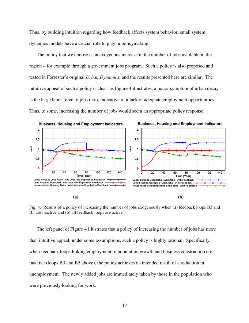
Thus, by building intuition regarding how feedback affects system behavior, small system
dynamics models have a crucial role to play in policymaking.
The policy that we choose is an exogenous increase in the number of jobs available in the
region – for example through a government jobs program. Such a policy is also proposed and
tested in Forrester’s original Urban Dynamics, and the results presented here are similar. The
intuitive appeal of such a policy is clear: as Figure 4 illustrates, a major symptom of urban decay
is the large labor force to jobs ratio, indicative of a lack of adequate employment opportunities.
Thus, to some, increasing the number of jobs would seem an appropriate policy response.
(a) (b)
Fig. 4. Results of a policy of increasing the number of jobs exogenously when (a) feedback loops B3 and
B5 are inactive and (b) all feedback loops are active
The left panel of Figure 4 illustrates that a policy of increasing the number of jobs has more
than intuitive appeal: under some assumptions, such a policy is highly rational. Specifically,
when feedback loops linking employment to population growth and business construction are
inactive (loops B3 and B5 above), the policy achieves its intended result of a reduction in
unemployment. The newly added jobs are immediately taken by those in the population who
were previously looking for work.
Business, Housing and Employment Indicators
2
1.5
1
0.5
0
33 3
33 3 3 3 3 3
2
2
2 2 2 2 2 2 2 21 1
11 1 1
1 1 1 1 1
0 20 40 60 80 100 120 140Time (Year)
dm
nl
Labor Force to Jobs Ratio : Add Jobs - with Feedback 1 1 1Land Fraction Occupied : Add Jobs - with Feedback 2 2 2 2Households to Housing Ratio : Add Jobs - with Feedback 3 3 3
Business, Housing and Employment Indicators
2
1.5
1
0.5
0
33 3
33 3 3 3 3 3
2
2
2 2 2 2 2 2 2 21 1
11 1 1
1 1 1 1 1
0 20 40 60 80 100 120 140Time (Year)
dm
nl
Labor Force to Jobs Ratio : Add Jobs - No Population Feedback 1 1Land Fraction Occupied : Add Jobs - No Population Feedback 2 2Households to Housing Ratio : Add Jobs - No Population Feedback 3 3

18
Reactivating the two feedback loops, however, illustrates how feedback can undermine even
the most well intentioned policies. As before, the exogenous increase in the number of jobs
immediately leads to a decrease in the ratio of labor to job opportunities. However, feedbacks
B3 and B5 create substantial policy resistance over time. Specifically, the increase in the
number of jobs (combined with still plentiful housing) raises the attractiveness of the region,
causing an increase in the population that overwhelms the new employment opportunities. At
the same time, the initial increase in jobs reduces slightly the pressure to build more business
structures, resulting in a decline in the number of jobs available through normal means, thereby
undermining any gains in unemployment. Both mechanisms are examples of compensating
feedback that returns the system to its original state of stagnation. Thus, the small urban model
illustrates clearly how policy resistance, combined with overconfident policymakers who fail to
take an endogenous perspective, can lead to suboptimal outcomes.
The central insight of Urban Dynamics, preserved in the small version, is that the total
attractiveness of an urban region must be considered relative to the attractiveness of all
surrounding regions (Forrester, 1971b). If the attractiveness of a region increases temporarily
relative to others – for example if new employment opportunities are added, then somehow
attractiveness must fall until equilibrium is again reached. To solve the problem of urban
stagnation and decay, Forrester recommends policies that increase business structures and reduce
the stock of available housing, thereby balancing any change to overall attractiveness. In the
URBAN1 model, such a policy can be tested by adding a zoning system to the model that
reserves land for business structures as needed to support the population. Only by examining
such a policy in light of the full set of relationships between housing, population, and business
structures can policymakers hope to have success.

19
A second key insight is that the decay phase comes from natural asymmetries in the structure
and dynamics of business structures and housing. Housing in URBAN1 is assumed to last longer
and to be easier to construct in the built-up city. If those two differences between housing and
business structures are eliminated, urban decay does not result in URBAN1 (although
unemployment still rises). This insight, suggesting urban renewal policies that shift the bias
away from non-job-generating structures (e.g., housing) to job-generating structures, is
reasonably easy to see in URBAN1 and almost impossible to draw out of the full Urban
Dynamics model.
Urban Dynamics remains a classic example of system dynamics successfully applied to an
important public policy problem. A small version of the model can help to build and
communicate insight regarding the complex nature of urban systems, while preserving many of
the central lessons that a more disaggregated model would bring.
Model #2: The “swamping insight” model
In 1996, then President Bill Clinton signed the Personal Responsibility and Work
Opportunity Reconciliation Act to change the role of the federal government in providing
support for poor families. The legislation replaced programs providing the potential of lifetime
federal support for indigent families with Temporary Assistance to Needy Families (TANF).
Passing this law shifted responsibility to individuals, states and counties, and made many local
government agencies more concerned with welfare issues. For policymakers and researchers
also, the condition was new and difficult to fully address (Zagonel et al. 2004; Richardson,
2006).

20
In January of 1997, Aldo Zagonel, John Rohrbaugh, George Richardson and David
Andersen1 were involved in a simulation project with a coalition of New York State agencies and
three county governments to address state level policymaking issues in regard to TANF. The
project is reported in several articles including Zagonel et al. (2004), Richardson et al. (2002)
and Richardson (2006). In addition to playing an important role in developing and testing
different policies at the state level, the project was also one of the cases used to develop more
general processes of group model building (Richardson and Andersen, 1995; Vennix, 1996;
Andersen and Richardson, 1997). Overall, several conceptual and simulation models that
address different state level polices were created.
One of the models that emerged is a small system dynamics model that examines the effect
of investment in the different parts of the system. This piece, like the other sets of models that
were developed, is grounded in the qualitative data extracted through a group model building
process. Some insights from the model are reported in Richardson et al. (2002) and Richardson
(2006). This model - later referred to as the “swamping insight” model - can be considered a
common archetype of systems that include recidivism.
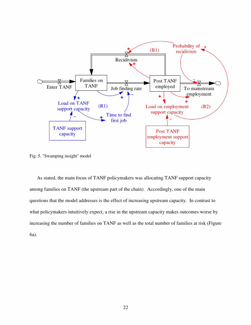
The model, shown in Figure 5, uses an aging chain structure to represent the flow of potential
recipients of TANF support, i.e. total families at risk. The chain includes two main stock
variables, Families on TANF and Post TANF employed. Families on TANF receive TANF
support, while those in the Post TANF employed stock remain at risk but do not receive direct
support. While families on TANF are at the center of the attention of TANF policymakers, a
holistic view to the problem suggests that policymakers should consider all at-risk families,
including both those that are in the program and those that may return to the program. The
number of families on TANF increases as families enter the program and decreases as they find
1 ordered as appeared in Zagonel et al. 2004
21
employment and move to the post TANF employed stock. Most of the individuals from post
TANF employed families are employed in low wage and temporary jobs. Thus, these families
are still at risk of recidivism and can return to the former stage (Families on TANF) if individuals
lose their job.
The modelers formulated the flow rates based on two variables representing supportive
capacities in the system. TANF support capacity influences the Job finding rate such that as
support capacity increases, people find jobs more quickly and move to the next stage. A similar
effect exists for the downstream capacity (Post TANF employment support capacity), which
captures the economic condition of the region and number of jobs available for post TANF
families. Usually post TANF jobs are low wage or temporary jobs, and post TANF families
therefore face a high risk of losing employment and returning to a state of need. Alternatively,
families may graduate from post TANF employment into mainstream employment, after which
they hold much greater job security. We assume that once families enter mainstream
employment they will not need (and will not be eligible for) any future TANF assistance. The
model captures the recidivism phenomenon by defining a variable named Probability of
recidivism as a function of the Post TANF employment support capacity. As this capacity
increases more people exit the chain of people at risk and enter mainstream employment and
fewer return to the TANF program.2 We will discuss the results of sensitivity analysis regarding
the elasticity of the Probability of recidivism later.
2 The outflows from the Post TANF employed stock are formulated as follows:
Recidivism = (Post TANF employed/Time in post TANF employed)* Probability of recidivism
To mainstream employment = (Post TANF employed/Time in post TANF employed)* (1-Probability of
recidivism).
The Time in post TANF employed (not represented in figure 5) is set to 10 Months. The Time to find first job is
assumed to be equal to 6 months when the Load on TANF support capacity is equal to 1.
22
Families onTANF
Post TANFemployedJob finding rate
Recidivism
Post TANFemployment support
capacity
Load on employmentsupport capacity
-
Probability ofrecidivism
+
TANF supportcapacity
Time to findfirst job
Load on TANFsupport capacity
-
-To mainstream
employment
-
Enter TANF
(R1) (R2)
(B1)
++
+
+
+
+
+
Fig. 5. "Swamping insight" model
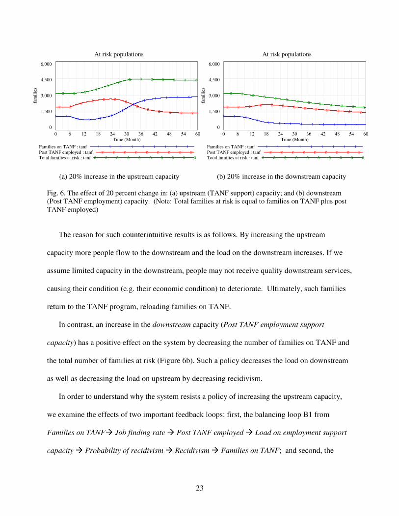
As stated, the main focus of TANF policymakers was allocating TANF support capacity
among families on TANF (the upstream part of the chain). Accordingly, one of the main
questions that the model addresses is the effect of increasing upstream capacity. In contrast to
what policymakers intuitively expect, a rise in the upstream capacity makes outcomes worse by
increasing the number of families on TANF as well as the total number of families at risk (Figure
6a).
23
(a) 20% increase in the upstream capacity (b) 20% increase in the downstream capacity
Fig. 6. The effect of 20 percent change in: (a) upstream (TANF support) capacity; and (b) downstream
(Post TANF employment) capacity. (Note: Total families at risk is equal to families on TANF plus post
TANF employed)
The reason for such counterintuitive results is as follows. By increasing the upstream
capacity more people flow to the downstream and the load on the downstream increases. If we
assume limited capacity in the downstream, people may not receive quality downstream services,
causing their condition (e.g. their economic condition) to deteriorate. Ultimately, such families
return to the TANF program, reloading families on TANF.
In contrast, an increase in the downstream capacity (Post TANF employment support
capacity) has a positive effect on the system by decreasing the number of families on TANF and
the total number of families at risk (Figure 6b). Such a policy decreases the load on downstream
as well as decreasing the load on upstream by decreasing recidivism.
In order to understand why the system resists a policy of increasing the upstream capacity,
we examine the effects of two important feedback loops: first, the balancing loop B1 from
Families on TANF� Job finding rate � Post TANF employed � Load on employment support
capacity � Probability of recidivism � Recidivism � Families on TANF; and second, the
At risk populations
6,000
4,500
3,000
1,500
0
3 3 33
33
3 3 3 3 3 3 3
2 22
2 2 22
22
2 2 2 21 1
1 1 11
1
11
1 1 1 1
0 6 12 18 24 30 36 42 48 54 60
Time (Month)
fam
ilie
s
Families on TANF : tanf 1 1 1 1 1 1 1 1 1
Post TANF employed : tanf 2 2 2 2 2 2 2 2 2
Total families at risk : tanf 3 3 3 3 3 3 3 3 3 3
At risk populations
6,000
4,500
3,000
1,500
0
3 3 3 3 3 3 3 3 3 3 3 3 32 2 2 2 2 2 2 2 2 2 2 2 21 1 1
11 1 1 1 1 1 1 1 1
0 6 12 18 24 30 36 42 48 54 60
Time (Month)
fam
ilie
s
Families on TANF : tanf 1 1 1 1 1 1 1 1 1
Post TANF employed : tanf 2 2 2 2 2 2 2 2 2
Total families at risk : tanf 3 3 3 3 3 3 3 3 3 3
24
reinforcing loop R2 from Post TANF employed � Load on employment support capacity �
Probability of recidivism � To mainstream employment � Post TANF employed. As defined by
these feedback loops, the probability of recidivism is an endogenous variable that changes as a
function of load on employment support capacity.
The effect of loops B1 and R2 on system behavior can be illustrated by changing the
functional relationship between the Load on employment support capacity and the Probability of
recidivism. Figure 7 shows three different functional forms, listed as scenarios. In Scenario 1
(the base run), the function is formulated based on data from the expert meetings. In Scenario 2,
we assume that both feedback loops are broken and that the probability of recidivism is a
constant number. This scenario is equivalent to a partial model test that illustrates the rationality
of decision makers assuming an absence of feedback through the probability of recidivism. In
Scenario 3, we reintroduce feedback, but decrease the gain of the loops by changing the
sensitivity of probability of recidivism to load on employment. The third scenario shows how the
system will behave if the probability of recidivism is not as sensitive to load on employment as
in the base run, but still varies endogenously.

25
(a) (b)
Fig. 7. (a) Different scenarios for how load on employment support capacity influences probability of
recidivism and (b) corresponding simulation results for Families on TANF
Figure 7 shows that the above mentioned feedback loops play significant roles in simulation
results. When in the second scenario we assume a constant probability of recidivism (no
feedback through this variable), we see that as policymakers expect, an increase in the upstream
capacity results in a decrease in Families on TANF. Thus, the reason that the system resists an
increase in upstream capacity in the base run is the effect of an increase in probability of
recidivism, which in turn decreases the outflow from Post TANF employed to mainstream
employment (labeled To mainstream employment), and increases the outflow from Post TANF
employed to Families on TANF (labeled Recidivism). Interestingly in the third scenario Families
on TANF ends up in a higher equilibrium.3
3 The system can also produce some interesting oscillatory behaviors under some specific conditions, but discussion
on all possible modes of behavior of this model is out of the scope of this paper.
0
0.25
0.5
0.75
1
0.5 0.75 1 1.25 1.5
Load on employment support capacity
Pro
ba
bil
ity
of
rec
idiv
ism
Scenario 1:
Base run
Scenario 2
Scenario 3
4,500
3,375
2,250
1,125
0
0 180 360 540 720 900 1080
Time (Month)
fam
ilie
s
Scenario 1:
Base run
Scenario 2
Scenario 3
Simulation results: Families on TANF Scenarios

26
Naturally, policymakers are prone to concentrate on the part of the system for which they are
most responsible. After focusing more and more people at the upstream and in the absence of a
holistic view of the system, policymakers may attribute worsening outcomes to exogenous
influences. In reality, it is their own policy that has reduced downstream services and raised the
level of recidivism. The final equilibrium level of at-risk families is an important concern for
policymakers and this model is able to show how various investments influence that level. To
that end, we conduct sensitivity analysis for changes in capacity at upstream and downstream
and plot the final equilibrium stage versus changes in these capacities. (Figure 8)
(a) (b)
Fig. 8. The equilibrium stage for (a) families on TANF and (b) total families at risk versus changes in
upstream (TANF support) capacity and changes in downstream (post TANF employment) capacity
Figures 8a and 8b show that an increase in downstream capacity always leads the whole
system to be better off while a change in the upstream capacity, if is not followed by a proper
level of increase in the downstream capacity, can make the whole system worse off.
00.05
0.10.15
0.2
0
0.05
0.1
0.15
0.2
0.25
0.3
0.35
0.4
1000
1500
2000
2500
3000
3500
4000
4500
5000
5500
change in downstream
capacity
change in upstream
capacity
Total
families
at risk at
t = 60
month
00.05
0.10.15
0.2
0
0.05
0.1
0.15
0.2
0.25
0.3
0.35
0.4
0
500
1000
1500
2000
2500
3000
3500
4000
change in downstream
capacity
change in upstream
capacity
Families
on TANF
at t = 60
month
27
Overall, this small model shows that adding capacity upstream can swamp downstream
resources, increasing the recidivism rate and resulting in still more demand upstream. In other
words, adding capacity upstream, by itself, can increase the upstream load and make the entire
system worse off (Richardson et al., 2002). This simple model helps policymakers: 1) develop a
holistic view of their problem, 2) better understand counterintuitive lessons from the model, 3)
experiment to find better policies for implementation in the real world, and 4) learn about
swamping insight and the endogenous causes of policy failure.
The Common Characteristics of Small System Dynamics Models
As discussed above, public policy problems have several characteristics (the “problems” of
public policy problems) that make effective policy making especially difficult. Yet, by
examining small system dynamics models like the URBAN1 model and the swamping insight
model, important insights regarding the source of policy failures can be uncovered. In this
section, we highlight common characteristics of the two models and discuss how small system
dynamics models can contribute to public policy making more generally. The discussion is
summarized in Table 1.
We argue that four central characteristics make small system dynamics models especially
well suited for learning about and designing effective policies: 1) the feedback approach and
emphasis on endogenous explanations of behavior, 2) the aggregate approach, 3) the simulation
approach, and 4) the fact that the models are “small” enough such that the structure is clear and
the link between structure and behavior can be easily discovered through experimentation. We
next explore each of these four characteristics in turn.

28
Feedback approach
First, both URBAN1 and the swamping insight model share a feedback loop approach to
modeling that emphasizes endogenous sources of behavior. The URBAN1 model illustrates how
housing and business construction policies that are effective during a period of growth can
endogenously create the conditions for decay once land becomes scarce, by causing an excess of
housing relative to the region’s employment capacity. Similarly, the swamping insight model
shows how increasing resources allocated to upstream welfare services can result in even greater
demand for such services by overloading downstream capacity. In both cases, the problem
behavior is endogenously created and is highly counterintuitive.
Such counterintuitive behavior is often an example of policy resistance. Too often, policies
fail due to unanticipated compensating feedback. For example, adding jobs to an urban area may
fail to improve unemployment if the increased attractiveness causes more people to move into
the area. By emphasizing feedback and an endogenous perspective, both models help
policymakers understand how policy resistance can arise. Both models challenge common
beliefs about how systems work by revealing feedback loops that can exacerbate the situation,
thereby facilitating learning for even the most overconfident users.
Aggregate approach
Second, both URBAN1 and the swamping insight model take an aggregate approach to
modeling. More specifically, neither model tracks each individual in the population separately,
but instead models groups of individuals in the aggregate. In keeping with the system dynamics
modeling tradition, the building blocks of model structure are stocks and flows rather than
individual agents. The urban model has one stock for population, another for housing structures,

29
and a third for business structures. Likewise, the swamping insight model has one stock each for
upstream and downstream welfare service recipients. Both models neglect any more detailed
implications that might arise due to agent heterogeneity.
While there is a huge interest among modelers in a disaggregated approach to the modeling
of social problems, Rahmandad and Sterman (2008) argue that differential equation-based
models – of which the models here are examples – are easier to understand and usually have
similar policy implications. In addition, aggregation reduces the size of the model, thereby
decreasing the cost of developing and running models and allowing for more experimentation.
Given limitations in individuals’ cognitive capacity, aggregation also allows users to focus on
feedback ahead of agent level detail and therefore develop a more holistic and endogenous
perspective to the problem.
Further, recent research has shown that individuals often fail to understand the dynamics of
accumulation (Sterman, 2008), with huge implications for the policies that they will then
support. By focusing on stocks and flows as the building blocks of model structure, system
dynamics models can directly help policymakers build intuition regarding the dynamics of
accumulation and thereby overcome one potential source of policy error.
Simulation approach
Third, both of the reviewed models are running mathematical simulations that provide the
opportunity to conduct experiments. While many lessons can be learned from a paper causal loop
diagram, other more substantial insights require the development and testing of a simulation
model. In both of the above cases, simulation helps to illustrate why intendedly rational policies
lead to policy resistance.

30
Further, simulation models provide learning environments where modelers, policymakers,
and others can design and test policies. Given the complexity of many policy environments,
experimentation is essential for the design of effective policies. Simulations provide a helpful
environment where policymakers can experiment and learn about the effects of different policies
without any significant social and economic cost for policymakers.
Finally, simulations can help to build consensus surrounding difficult policy problems. By
communicating the counter-intuitive nature of policy problems to policymakers, simulations can
encourage dialogue and lead to the development of shared interpretations regarding the source of
problem behavior. Even when different goals and value systems persist, simulation can help to
focus the discussion on specific variables and outcomes that are the source of divergence.
Small model size
Finally, both of the models are “small.” Here, we define “small” to mean models that consist
of a few significant stocks and at most seven or eight major feedback loops. There are two main
benefits to a small size. First, a small model size allows for exhaustive experimentation through
parameter changes. With lower order models it is much easier to learn from sensitivity analysis
(as shown in the swamping insight model, Figures 7 and 8) and examine the interactions among
different parameters. Thus, important leverage points in the system can be more easily identified.
Second, a small size ensures that the results of experiments can be fully and easily
understood by policymakers. Short exposition makes a holistic view possible. Due to the small
size, individuals can see the feedback structure as a whole and not be frustrated by the need to
track many variables and links at once. In addition, short exposition facilitates presentation of
lessons to others, and helps bring the dynamic lessons to the meetings of stakeholders. Our

31
emphasis on small models echoes that of Repenning (2003), who argues that in an academic
context as well, small models are necessary to build the intuition of readers who are not
accustomed to a dynamic or holistic view of systems.
All told, small system dynamics models bring numerous benefits to the public policy making
process. Table 1 summarizes the above discussion by depicting how each of the characteristics
of small system dynamics models can help address the challenges inherent in public policy
making.

32
Table 1. The significance of small system dynamics models in addressing public policy problems
Small system dynamics models characteristics
Feedback Approach Aggregate approach
(Stock-Flow) Simulation Approach Small Model Size
The policy resistance
environment
Feedback is the major source
of policy resistance.
Accumulations (stocks) are
essential to understanding policy
resistance.
Simulation can illustrate why some
intuitive policies lead to policy
resistance and allow for the design
and testing of more robust policies
Small size allows for exhaustive
experimentation and sensitivity
analysis, wise interpretation of
parameters and parameter changes.
Need to experiment
and cost of
experimenting
Feedback diagrams and
mental simulation (thought)
must substitute here for actual
policy trials.
Aggregate approach decreases
the cost of developing and
running models, allowing for
more experimentation.
Simulations allow for exhaustive
experimentation and games for
policymakers without incurring
actual social and economic costs.
Small size ensures that the results
of experiments can be fully and
easily understood by policymakers.
Need to persuade
different stakeholders
Feedback diagrams and
qualitative analysis can
contribute to policy
discussions.
Aggregate approach facilitates
presentation of lessons to others.
Highlights feedback and
endogenous sources of problem
behavior.
Simulations can help build
consensus around difficult policy
problems that may otherwise have
multiple interpretations.
Small size facilitates presentation
of lessons to others. Short
exposition and holistic view made
possible.
Overconfident
policymakers
Causal loop (feedback)
diagrams reveal new insights
and challenge policymakers
to be wary of overconfidence.
Failure to understand the
dynamics of accumulation is a
common source of policy error.
Simulations effectively
communicate the counter-intuitive
nature of policy problems to
policymakers who otherwise may
remain unpersuaded.
Small size ensures that model
insights are fully understood,
allowing policymakers to
appreciate and address their own
overconfidence.
pu
bli
c p
oli
cy p
rob
lem
s ch
ara
cter
isti
cs
Need to have an
endogenous
perspective
Feedback approach helps
policymakers learn what an
endogenous view is and why
it is necessary to effective
policymaking.
Aggregate approach leaves more
room in individuals’ cognitive
capacity to concentrate on
feedback and develop an
endogenous perspective.
Simulations allow policymakers to
explore how behaviors are created
endogenously through a broad
model boundary.
Small size allows individuals to
see the feedback structure as a
whole and not be frustrated by the
need to track many variables and
links at once.

33
Conclusion and discussion
In this paper we argued that small system dynamics models can be very helpful for policy
making. After listing several common difficulties in policy making, we next reviewed two
insightful models and used these models as examples to examine how small system dynamics
models can address some of the most pressing challenges that policymakers face.
We believe that small system dynamics models can contribute significantly to policy making
due to four central characteristics: first, they take a feedback approach; second, they are
aggregated; third, they present simulation runs; and fourth, they are “small.” Because of these
characteristics, small system dynamics models can illustrate the sources of policy resistance in
the environment, facilitate learning through extensive experiments, overcome the issues of
overconfidence, bring different stakeholders to a shared understanding, and help policymakers
learn about the importance of an endogenous perspective to problem solving.
Despite these benefits, it is important to mention that small models do also have limitations.
First, customers in general and policymakers in particular often demand an exclusive model that
considers all possible causal links either observed or contemplated. In such a situation,
policymakers may lose their trust if they see that their hypothesized link or variable does not
exist in the model. Further, in many situations, stakeholders may want to see their own
organizations, departments, or communities separately represented, increasing the level of
disaggregation. In such a case, having an exclusive version of the model and showing that the
final behavior is not qualitatively sensitive to the policymakers’ assumed important links or
variables can be helpful. Once the insights provided by a small model are well understood, a
more detailed model can be constructed to analyze more fine grained policy implications.
34
A further limitation is that the use of small models may lead modelers to underestimate the
role of some feedback loops which may actually be important in reality. It is critical to mention
that effective small system dynamics models must not only be simple, but also include all of the
most dominant loops. As a result, the process of building small models may in fact be more
difficult than building larger models that include multiple feedback loops. In many cases, small
models may emerge only after extensive examination of a larger model allows for the
identification and isolation of only the most dominant feedback loops. Once a large model is
developed and the modeler gets a clear idea of the dominant loops, he or she can build a smaller
version to present for policymakers.
Furthermore, building small models should not impede “operational thinking” and
modeling. System dynamics encourages thinking clearly about causalities and how variables
actually are connected to produce behavior (Richmond, 2001). Modelers should be clear in how
a variable ultimately influences another variable by stating step by step the path of the causal
link. Being precise in the formulation of causal links and clarifying important capacity
constraints are essential aspects of good modeling practice. Although small models may omit
some of the details behind causal links, variables can and must remain operational at a high level.
Overall, despite these limitations, we argue that small system dynamics models can greatly
aid the policymaking process. Small models help policymakers learn about the environment and
the sources of policy resistance, build learning environments for experimentation, overcome
overconfidence, and develop shared understanding among stakeholders. For all of these reasons,
we believe that the system dynamics community should do more to help policymakers
incorporate the use of small system dynamics models into the policymaking process.

35
Supporting Information
Supporting information may be found in the online version of this article.
References
Alberts B. 2008. A Scientific Approach to Policy. Science 322(5907): 1435.
Alfeld LE, Graham AK. 1976. Introduction to Urban Dynamics. Pegasus
Communications:Waltham, MA.
Andersen DF, Richardson GP. 1997. Scripts for Group Model Building. System Dynamics
Review 13(2): 107-129.
Babcock L, Loewenstein G. 1997. Explaining Bargaining Impasse: the Role of Self-Serving
Biases. Journal of Economic Perspectives 11(1): 109-26.
Bazerman MH. 1994. Judgment in managerial decision making, 3rd edition. Wiley: London.
Bretschneider S, Straussman J. 1992. Statistical Laws of Confidence Versus Behavioral
Response: How Individuals Respond to Public Management Decisions Under
Uncertainty. Journal of Public Administration Research and Theory 2(3): 333-34.
Cavana RY, Clifford LV. 2006. Demonstrating the utility of system dynamics for public policy
analysis in New Zealand: the case of excise tax policy on tobacco. System Dynamics
Review 22(4): 321-348.
Cyert RD, March JG. 1963. A Behavioral Theory of the Firm. Prentice-Hall: Englewood Cliffs,
NJ.
Denrell J, March JG. 2001. Adaptation as Information Restriction: The Hot Stove Effect.
Organization Science 12(5): 523-538.
Fiddaman TS. 1997. Feedback Complexity in Integrated Climate-Economy Models. Doctoral
Thesis, Massachusetts Institute of Technology, Cambridge, MA.
Fiddaman TS. 2002. Exploring policy options with a behavioral climate-economy model. System
Dynamics Review 18(2): 243-267.
Ford A. 1997. System Dynamics and the Electric Power Industry. System Dynamics Review
13(1): 57–85.
Ford A. 2005. Simulating the Impacts of a Strategic Fuels Reserve in California. Energy Policy
33: 483–498.

36
Forrester JW. 1969. Urban dynamics. MIT Press: Cambridge, MA.
Forrester JW. 1971a. World Dynamics. Wright-Allen Press: Cambridge, MA.
Forrester JW. 1971b. Counterintuitive behavior of social systems. Technology Review 73(3): 52-
68.
Forrester JW. 2007. System dynamics - the next fifty years. System Dynamics Review 23(2-3):
359 – 370.
Ghaffarzadegan N. 2008. How a System Backfires: Dynamics of Redundancy Solution in
Security. Risk Analysis 28(6): 1669 - 1687.
Griffin D, Tversky A. 1992. The weighing of evidence and the determinants of confidence.
Cognitive Psychology 24(3): 411–535.
Henrion M, Fischhoff B. 1986. Assessing uncertainty in physical constants. Journal of Physics
54(9): 791-798.
Homer J, Hirsch G, Milstein B. 2007. Chronic Illness in a Complex Health Economy: The Perils
and Promises of Downstream and Upstream Reforms. System Dynamics Review 23(2-3):
313-343.
Homer J, Ritchie-Dunham J, Rabbino H, Puente L, Jorgensen J, Hendricks K. 2000. Toward a
Dynamic Theory of Antibiotic Resistance. System Dynamics Review 16(4): 287-319.
Homer J, Hirsch G, Minniti M, Pierson M. 2004. Models for Collaboration: How System
Dynamics Helped a Community Organize Cost-Effective Care for Chronic Illness.
System Dynamics Review 20(3): 199-222.
Honggang X, Mashayekhi AN, Saeed K. 1998. Effectiveness of infrastructure service delivery
through earmarking: the case of highway construction in China. System Dynamics Review
14(2-3): 221-255.
Hood C, Peters G. 2004. The Middle Aging of New Public Management: Into the Age of
Paradox? Journal of Public Administration Research and Theory 14(3): 267–282.
Johnson DP. 2004. Overconfidence and war: the havoc and glory of positive illusions. Harvard
University Press: Cambridge, MA.
Landsbergen D, Coursey DH, Loveless S, Shangraw RF Jr. 1997. Decision Quality, Confidence,
and Commitment with Expert Systems: An Experimental Study. Journal of Public
Administration Research and Theory 7(1): 131-157.
Lichtenstein S, Fischhoff B. 1977. Do those who know more also know more about they know.
Organizational Behavior and Human Performance 20: 159-183.
37
Lichtenstein S, Fischhoff B, Phillips LD. 1982. Calibration of probabilities: The state the art to
1980. In D. Kahneman, P. Slovic, & A. Tversky (Eds.), Judgments under uncertainty:
Heuristics and biases (pp. 306–334). New York: Cambridge University Press.
Light PC. 1997. The tides of reform: Making government work 1945–1995. Yale University
Press: New Haven, CT.
Martinez-Moyano IJ, Rich E, Conrad S, Andersen DF, Stewart TR. 2008. A Behavioral Theory
of Insider-Threat Risks: A System Dynamics Approach. ACM Transactions on Modeling
and Computer Simulation, 18(2), Article 7.
Mashayekhi AN. 1998. Public finance, oil revenue expenditure and economic performance: a
comparative study of four countries. System Dynamics Review 14(2-3): 189-219.
McKenzie CRM, Liersch MJ, Yaniv I. 2008. Overconfidence in interval estimates: What does
expertise buy you? Organizational Behavior and Human Decision Process 107(2): 179-
191.
Meadows DH, Meadows DL, Randers J, Behrens WW. 1972. The Limits to Growth. Universe:
New York.
Morecroft J. 1983. System Dynamics: Portraying Bounded Rationality. Omega 11(2): 131-142.
Moxnes E. 1998. Not only the Tragedy of the Commons: Misperceptions of Bioeconomics.
Management Science 44(9): 1234-1248.
Rahmandad H. 2008. Effect of delays on complexity of organizational learning. Management
Science 54(7): 1297-1312.
Rahmandad H, Repenning NP, Sterman JD. 2009. Effect of Feedback Delays on Learning.
System Dynamics Review 25(4): 309-338.
Rahmandad H, Sterman JD. 2008. Heterogeneity and network structure in the dynamics of
diffusion: Comparing agent-based and differential equation models. Management Science
54(5): 998-1014.
Repenning NP. 2003. Selling System Dynamics to (Other) Social Scientists. System Dynamics
Review 19(4): 303-327.
Repenning NP, Sterman JD. 2002. Capability traps and self-confirming attribution errors in the
dynamics of process improvement. Administrative Science Quarterly 47(2): 265–295.
Richardson GP. 1983a. An Interview with Jay Forrester. PLEXUS, System Dynamics News 2.

38
Richardson GP. 1983b. Heroin Addiction and its Impact on the Community. In Introduction to
Computer Simulation, a System Dynamics Approach, edited by N. Roberts et al.
Addison-Wesley: Reading, MA.
Richardson GP, Andersen DF, Wu YJ. 2002. Misattribution in Welfare Dynamics: the puzzling
dynamics of recidivism. In Proceedings of the 2002 International System Dynamics
Conference, Palermo, Italy, 28 July- 1 August.
Richardson GP. 2006. Concept Models, In Proceedings of the 2006 International System
Dynamics Conference, Nijmegen, The Netherlands, 23-27 July.
Richardson GP, Andersen DF. 1995. Teamwork in Group Model Building. System Dynamics
Review 11(2): 113-137.
Richardson GP. 2007. How to Anticipate Change in Tobacco Control Systems, in Greater Than
the Sum: Systems Thinking in Tobacco Control, edited by Best A, Clark PI, Leischow SJ,
Trochim WMK. National Cancer Institute, U.S. Department of Health and Human
Services, National Institutes of Health.
Richmond B. 2001. An Introduction to Systems Thinking, (ithink software), High Performance
Systems, Inc.
Saeed K. 1998. Towards Sustainable Development, 2nd Edition: Essays on System Analysis of
National Policy. Ashgate Publishing Company: Aldershot, England.
Senge P .1990. The Fifth Discipline: The Art And Practice Of The Learning. Doubleday: New
York.
Sterman JD. 1989. Modeling Managerial Behavior: Misperceptions of Feedback in a Dynamic
Decision Making Experiment. Management Science 35(3): 321-339.
Sterman JD. 2000. Business dynamics: systems thinking and modeling for a complex world.
Irwin/McGraw-Hill: Boston, MA.
Sterman JD. 2008. Risk Communication on Climate: Mental Models and Mass Balance. Science
322 (24 October): 532-533.
System Dynamics Society. 2009. System Dynamics Bibliography.
http://systemdynamics.org/biblio/sdbib.html [1 June 2009].
Thompson KM, Duintjer Tebbens RJ. 2007. New Analysis Says Eradicating Polio a Better
Option Than Extended Control of the Disease. The Lancet 369:1363-1371.
Thompson KM, Duintjer Tebbens RJ. 2008. Using system dynamics to develop policies that
matter: global management of poliomyelitis and beyond. System Dynamics Review
24(4):433-449.

39
Thomson Reuters. 2009. ISA web of knowledge. http://www.isiwebofknowledge.com [20
September 2009].
Tversky A, Kahneman D. 1974. Judgment under Uncertainty: Heuristics and Biases. Science
185(4157): 1124-1131
Vennix J. 1996. Group Model Building: Facilitating Team Learning. Wiley: Chichester.
Weaver EA, Richardson GP. 2006. Threshold setting and the cycling of a decision threshold.
System Dynamics Review 22(1): 1-26.
Zagonel AA, Rohrbaugh JW, Richardson GP, Andersen DF. 2004. Using simulation models to
address ‘What If’ questions about welfare reform, Journal of Policy Analysis and
Management 23(4): 890-901.