Maxim > App Notes > Automotive

Keywords: UHF antenna, RKE, remote keyless entry Mar 26, 2006

APPLICATION NOTE 3621

Small Loop Antennas: Part 1—Simulations and Applied Theory

Abstract: Small-aperture UHF antennas for remote-keyless-entry (RKE) applications can be terminated either as a shorted or open loop within a fob. Depending on how the loop is terminated, its far-field pattern and the antenna's characteristic impedance will be influenced. In this application note we will explore antenna theory and design using EZNEC, an easy-to-use antenna simulator. We will measure the antenna's characteristic impedance through our application board. The results will show the tradeoffs between open and shorted loops, the effects of the ground, and considerations for antenna matching. All this information is a preface to the measurement described in Part II of this application note.

Contents

1. Antenna Environment 2. Maxim Antenna Experiment

2.1. Discussion of Methodology 3. Free Space and Practical Applications 4. Short vs. Open Loop

4.1. Shorted-Loop Case 4.1.1. Shorted Loop, 3D, Far Field at the Fundamental 4.1.2. Measured Impedance of a Shorted Loop 4.2. Open-Loop Case 4.2.1. Measured Impedance of an Open Loop

5. Spurious and Harmonic Antenna Considerations 6. Summary

1. Antenna Environment

Remote-keyless-entry (RKE) antennas are electrically short due to tiny package requirements and a relatively long wavelength at 300MHz to 400MHz. Ideally a simple and efficient RKE antenna is either a 1/2 wave dipole or a 1/4 wavelength monopole with its associated ground plane that mirrors the radiating element. Such an ideal configuration, however, would consume the space of a basketball and is, therefore, impractical for a tiny key fob activated between the user's fingers. As the radiating element is shortened to meet the fob's package requirements, the efficiency and impedance become poor and difficult to manage. Such constrained configurations can easily result in antenna losses due to reduced radiation efficiencies, plus component matching losses that are on the order -14dB¹. Harmonics, by definition, will have shorter wavelengths by 1/n, so the antenna radiation efficiency becomes better as the harmonic order increases. Under FCC regulations part 15.231, the emissions are measured in terms of field strength. Consequently, a small antenna aperture causes the opposite of what is desired. Testing for FCC compliance typically involves either the FCC directly or a laboratory accepted by the FCC performing exhaustive field-strength measurements in a controlled environment with agreed standards. Usually those tests are conducted on a wooden table to support the transmitter; no consideration is given for the field interaction of someone holding the fob or for the ground effects to field. Many testing facilities cannot take 3-D measurements and are only concerned with the worst case, reflected ground return that interferes with the direct ray. But in actuality, the ground can not only interfere with the measuring antenna, but also significantly affect the transmitter pattern itself. Antenna testing accounts for these ground effects by measuring the peak lobe in space and measuring a 360-degree field pattern around the antenna.

Page 1 of 23

Inexpensive yet powerful antenna simulators available to the public at reasonable cost can account for the ground effects, but usually not the effects of a lossy dielectric associated with holding the fob. Simulators work by dividing the elements into theoretical currents and then summing the results in the far field by a technique called 'method of moments.' Even for the simplest of antennas, the simulator's task is extremely difficult; there is usually no closed-form model, so it relies on lookup tables from measured data. For accurate antenna simulation, a great deal depends on having a mathematical current gradient within each calculated segment. EZNEC, which is simple hobbyist-grade, inexpensive antenna software, has a NEC2 core which allows the user to model tiny antennas and gives interesting results in the far field. EZNEC results are both useable and very helpful for understanding what is really occurring. NEC will also calculate the antenna impedance. For small antenna apertures, however, a negative resistance result is both usual, and an alert to a simulation error caused by ill-condition matrix math. NEC is ideally suited for dipoles and monopoles since it uses lookup tables from measured models to calculate the result. NEC's internal mathematical precision is not that high, so matrix multiplications can propagate errors for small-loop designs. Another modeling program, EIGER, is perhaps better suited for small antenna apertures, but not available to the public. After considering what software is available and inexpensive, we explored EZNEC's far-field simulation results for open and shorted antenna loops. We measured the impedance with an Agilent 8753D vector network analyzer. While the simulated results can appear conclusive, they only guide the designer in understanding what can be measured at an antenna range and what to expect when matching the device to the antenna. Information on various NEC versions and detailed hints for its uses can be found at State of the Art. EZNEC is available from Nittany Scientific² and more advanced versions (NEC-4) are available to US citizens through the Lawrence Livermore National Laboratories IPAC services³. There are also commercial high-end simulators such as Ansoft. Yet another possible simulator is WIPL-D4 code from Yugoslavia because it can model plates and strips over ground. While we have not explored the WIPL-D tool, it is available in the USA for about $400. These antenna simulators are powerful and reasonably priced. While powerful, these simulators are generally applied to larger antenna structures like dipoles, long wire, and Yaggi, etc., in typical outdoor settings. Modeling is very limited for tiny or printed antennas on dielectric media; even the latest advanced simulators like NEC-4 or EIGER5, which is available through government agencies, struggle with tiny loops on dielectric with ground planes as you would typically find in small RKE-type devices. Because these latter applications can easily go beyond the simulators' capabilities, measuring the antenna's result directly is the only true way to verify performance.

2. Maxim Antenna Experiment

A FR4 board with a typical printed-loop configuration extending from a key fob was fabricated and measured. The antenna was probably somewhat large for most applications, but it served well to help understand what was occurring with its impedance and EZNEC simulation.

Page 2 of 23

Figure 1. Maxim antenna board. To calibrate the network analyzer, a series of calibration standards (open, short, and 50Ω) were included on the board for 1-port S measurements. Although these calibration standards did not include coefficients from factory calibration kits, they worked quite well at 400MHz, requiring only a port extension to place the reference point at the feed point of the antenna. See Figure 1. The antenna was configured in two scenarios:

1. The opposite end shorted at A 2. The opposite end open at A

Measurements in S11 were taken with the antenna suspended as shown; its impedance was recorded. The board was also modeled in EZNEC to estimate the field pattern of the antenna. Verification of the actual field pattern, based on measurements done at an outside testing range at Elliot Laboratories in Sunnyvale, CA, will be explored in the second half of this application note 3622, "Small-Loop Simulation and Applied Theory Part 2—Field Tests." Figure 2 illustrates the Maxim board modeled in EZNEC. The magenta lines suspended above elements 1, 2, 3, 4...8 show the relative RF currents.

Figure 2. Modeling the 1in x 1in antenna loop with finite elements in EZNEC.

Page 3 of 23

2.1. Discussion of Methodology

With small loops, energy will seek a resonance to satisfy field-boundary conditions. The problem with using a coax to drive the device under test (DUT) is that the shield has a greater aperture than the actual active element being measured. The loop will effectively excite the coax's shield through the loop's ground return, much as RF is coupled by beta match on a Yaggi antenna. Through experimentation we found a sharp resonance while measuring S11, Figure 3 at R. Although sharp, the resonance was weak enough to be eliminated by squeezing the coax a distance away from the antenna without changing S11 at the desired measurement frequency. A ferrite bead (some refer to these as 'prayer beads') or current balun over the coax would have accomplished the same thing.

Figure 3. Resonance caused by coax shield. While the effects of the coax's ground resonance did not significantly affect S11 at our operating frequency, the currents excited on the ground plane did distort the measured field pattern. A more difficult, but potentially more accurate approach would optimize RF power which the Tx IC delivered to the antenna by changing the L-C match and then measuring the network to determine the impedance.

Figure 4. Fixture and EZNEC model during associated S-par measurements. Page 4 of 23

Since the loop was going to excite currents in the ground plane, EZNEC was also used to compare the error induced in the far field by a coax to the ideal case of the loop as an independent element in space. Results are shown in Figure 5.

Figure 5. Comparing modeled coax effects to the far field (shorted loop). As one would expect, there was an effective pulling of the far-field pattern in the direction of the coax. A curious effect was the change in field in the Z axis, probably attributed to changing the average height of the radiator above ground and coupling energy from the coax itself. In the case where there was no coax, the field pattern was more symmetrical over the circuit's ground plane.

3. Free Space and Practical Applications

One surprising simulation result is the very strong lobe along the Z axis for both the shorted and open termination in Figure 5. Since the loop is small and the current is uniform, one would expect a field pattern close to isotropic (Figure 6) or a slight distortion from the physical implementation of the active element, as shown in Figure 7.

Page 5 of 23

Figure 6. Neglecting effects of the coax in free space. In the free-space model we see the effects of the coax and the substantial energy in the -Z direction that can be reflected by the ground. Since the coax shield is longer than the antenna element, it will contribute to the far field like a long random-wire antenna.

Figure 7. Effect of the coax in free space (shorted loop). In our model, the coax shield element was arbitrarily fixed at 19 inches, which was slightly more than a 1/2 λ at 315MHz and about 3/4 λ at 433MHz. Considering that the shield acted as a monopole as a function of wavelength, the field became more directionally perpendicular to its axis as the length increased until 5/8 λ (0.625 λ). Beyond 5/8 λ, a new lobe below the main lobe started to form, thus sending the main lobe skyward. As the element lengthened, alternating lobes and nulls in elevation to the antenna axis resulted. Figure 8 shows both how these lobes and nulls merge in the far field when combined with the incident wave from the loop, and the distortions that resulted between 315MHz and 433MHz.

Page 6 of 23

Figure 8. Vertical monopole-elevation field pattern as a function of wavelength. While the results above are correct in free space, the effect of the ground is also an important factor which cannot be ignored. Reflections from ground add constructively and destructively to the incident wave, resulting in a varying lobe skywards. The differences of the Z-axis lobe between 315MHz and 433MHz are not so much the result of antenna directivity along the Z axis, but more from the additive phases of the incident and the reflected signals due to the differences in wavelength to ground. EZNEC was modeled in previous examples to have an ideal ground 36 inches above the X-Y plane (Figure 9), the typical height of a key fob when being used. If the distance of the antenna from ground changed, the lobe in the center predictably progressed through maxima and minima for each 1/4 λ above the ground.

Figure 9. Modeled loop above ground.

Page 7 of 23

Since the reflected wave's intensity follows 1/r4, the reflected wave will eventually contribute little to the incident that diminishes 1/r² in the far field. For practical RKE applications, EZNEC predicts that the ground will still have a significant influence on the field pattern of the antenna. The data are illustrated in Figure 10.

Figure 10. Effect of antenna height above ground, λ = 35.65 inches.

4. Shorted vs. Open Loop

Should the antenna have a shorted or open loop? Designers face this question either to find an easier matching result or to improve the antenna efficiency somehow. Often antennas can be approached as two tasks: first, select the aperture for desired radiation, and then match it to the generator. Occasionally an identical aperture can be treated the same when terminated differently, but the actual results in the antenna's field pattern can be quite different for a shorted or open loop, depending on how the currents distribute. See Figure 11.

Figure 11. Comparing antenna currents. In the shorted loop case which is less than 1/4 wavelengths, the boundary condition will be at the ground point forcing peak currents through the entire loop. The current will slowly change in phase from segment 1 to 4. In the case of an open loop, there is a break in the path resulting in no current at the gap and progressively larger currents moving toward the feed point. The current phase will start out the same from the break along segments 3 and 4, but also continue through segments 2 and 1. In either case, each segment will radiate a finite amount of energy from the currents in each segment. Depending on the position of the segment and the phase of the current that flows through, the vector sum of all the elements determines the field pattern in the far field. While a single open-ended element radiates a field very efficiently, in actuality it is a monopole mirrored by the ground completing the circuit to space. For a small fob exciting an open loop, there is virtually no ground element. Consequently, the PCB ground that is available becomes part of the antenna. In comparing open and shorted loops, the greatest difference will be the feed impedance since the termination is

Page 8 of 23

starting from opposite ends of the Smith chart (Figure 12). Such change in impedance could result in stability issues, if the active element attached to the antenna is not unconditionally stable. Maxim RKE transmitter devices are unconditionally stable. This is especially important since anything in close proximity to the antenna, such as metal or a thumb, will affect the antenna's impedance, thus possibly causing a device to oscillate.

Figure 12. Starting impedance of open and shorted loops and stability circles.

4.1. Shorted-Loop Case

A loop or coil carrying an alternating current will generate an alternating magnetic field perpendicular to the loop's plane. The same applies at UHF with a short loop. If, however, the loop is electrically long, the phase of the RF current traveling around it will be equivalent to a string of discrete antennas shifted in phase by the preceding element (Figure 13).

Figure 13. Equivalent multiple dipoles for a long loop. Each one of these effective antennas will start to interfere with, or contribute to the far field, thereby resulting in the pattern shown in Figures 14 and 15. For a loop circumference of less than 1/2 wavelengths, the current is relatively constant so the far-field intensity is directed along the X axis. In Figures 14 and 15, we kept the same mechanical

Page 9 of 23

dimensions of the 1in x 1in square loop in the X-Z plane and increased the excitation frequency. This approach accomplished two things. Firstly, it showed the relationship between wavelengths to a fixed 1-inch square loop, and secondly, it showed the effects of shorter wavelength harmonics.

Frequency Effective 4-inch circumference loop, length in wavelengths

10MHz 0.004 λ

100MHz 0.036 λ

315MHz 0.112 λ

433MHz 0.154 λ

700MHz 1/4 λ Figure 14. X-Y far-field patterns for an electrically short loop in free space. As the loop becomes electrically longer or until there is a discrete phase relationship with each leg, the far-field maxima will remain along the X axis. The first symmetrical boundary condition to be met is when the path around the loop is 180 degrees, also matching the 180 phase difference at the antenna's feed point. The result will be like a vertical half-wave dipole standing in the Z axis as shown for 1.4GHz in Figure 15 below.

Frequency Effective 4-inch circumference loop (length in wavelengths)

1.4GHz 1/2 λ

2.8GHz 1 λ

3.5GHz 1 1/4 λ

4.2GHz 1 1/2 λ

4.9GHz 1 3/4 λ

5.6GHz 2 λ

11.2GHz 4 λ Figure 15. X-Y far-field patterns for an electrically long loop in free space. Beyond 1/2 wavelengths (1.4GHz), the single loop will effectively have a greater phase shift in current as the loop's length increases. Since each side of the loop occupies a different point in space, a point that is significantly spaced from each other relative to its wavelength, the far-field result will progress as shown in Figure 15.

Page 10 of 23

Figure 16. Asymmetrical feed point of loop. Figures 14 and 15 illustrate several important points. All the simulations in these figures used the model in Figure 16, as a loop on a PCB was probably not perfectly symmetrical. Figure 16's model also matched closer to what was happening in our test fixture in Figure 4. Using a model with a slightly offset feed point demonstrates that for electrically short loops, the feed point's location is not too important since relative phase shift within the loop is insignificant. As the loop gets electrically longer due to shorter wavelengths, however, the phase of the current shift becomes more significant to the physical model, thus affecting the far field (note magenta current lines in Figure 17). If the feed point in Figure 16 (asymmetrically fed loop) was the same as in Figure 17 (symmetrically feed loop), the field patterns above 1 λ would be perfectly symmetrical...in some axis.

Figure 17. Gain and directional effects as loop becomes electrically long free space. If the loop is short for the fundamental, it will become longer for its harmonics. This is important since it is becoming clear how harmonics can result in unpredictable fields stronger than the fundamental, including polarization changes. The example in Figure 17 also illustrates that while we are studying the X-Y plane, having higher order harmonics can yield a maxima in a third dimension, in this case going skywards in the X-Z plane. This effect should not be surprising since the antenna also resembles a classic Rhombic antenna whose directive pattern will be opposite to the feed point.

Page 11 of 23

4.1.1. Shorted Loop, 3D, Far Field at the Fundamental

Figure 18. Shorted-loop far-field simulation without PCB ground plane. Figure 18 illustrates the simulated result for a small loop that neglects the PCB ground plane of our fixture shown in Figure 1. This condition is very similar to that found in an actual key fob, since such ground plane would be unavailable for a small package. By carefully comparing the differences between signals in free space and signals over ground, and by noting the differences in the Z axis at 315MHz and 433MHz, it is clear that the effects are ground-related, as discussed previously. The dimples in the free-space model can also be correlated to the minima in Figure 15 along the Y axis. When considering ground-plane effects as in the case of our test fixture in Figure 4, you will find that some of the currents are being pulled into the ground plane, thus yielding a contribution to the far field. Here the antenna is somewhat a hybrid of a loop and dipole because there is current along the edge of the ground at element 4. Some of this ground current will be induced in the ground plane much like an autotransformer. While the current is significantly less than in the loop, the ground has a much larger aperture area. The result is a change in effective height, because the antenna's effective center has been lowered causing the lobe along the Z axis to change between 315MHz and 433MHz.

Page 12 of 23

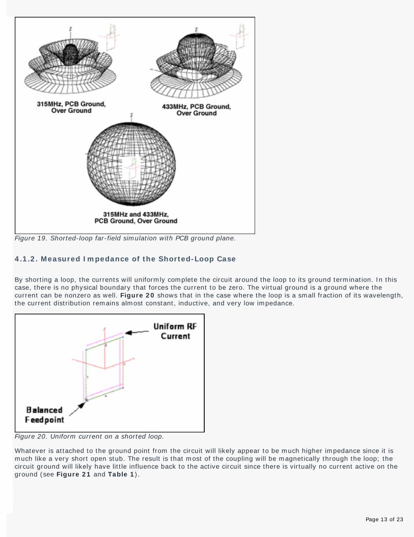
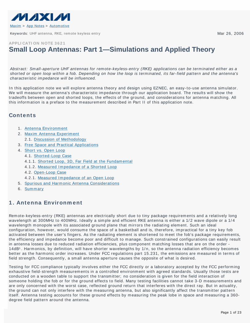
Figure 19. Shorted-loop far-field simulation with PCB ground plane.

4.1.2. Measured Impedance of the Shorted-Loop Case

By shorting a loop, the currents will uniformly complete the circuit around the loop to its ground termination. In this case, there is no physical boundary that forces the current to be zero. The virtual ground is a ground where the current can be nonzero as well. Figure 20 shows that in the case where the loop is a small fraction of its wavelength, the current distribution remains almost constant, inductive, and very low impedance.

Figure 20. Uniform current on a shorted loop. Whatever is attached to the ground point from the circuit will likely appear to be much higher impedance since it is much like a very short open stub. The result is that most of the coupling will be magnetically through the loop; the circuit ground will likely have little influence back to the active circuit since there is virtually no current active on the ground (see Figure 21 and Table 1).

Page 13 of 23

Figure 21. Measured spar for a shorted loop. Table 1. Measured Spar for A Shorted Loop for the 300MHz and 400MHz Bands Loop Antenna with shorted end to ground plane

F (MHz) S11 mU Deg Re-Ω Im-Ω S11x S11y

300.00 983.140 32.712 5.344 170.2 0.827 0.531

315.00 983.410 29.947 6.250 186.74 0.852 0.491

330.00 983.400 28.151 7.055 199.17 0.867 0.464

429.00 983.930 12.703 32.906 446.73 0.960 0.216

432.00 984.520 12.182 34.453 465.97 0.962 0.208

433.50 984.720 11.864 35.844 478.52 0.964 0.202

441.00 986.330 10.916 37.750 520.41 0.968 0.187

4.2. The Open-Loop Case

In the open-loop case, whatever main element is exposed will become the antenna, including the coax shield. When measuring a short monopole antenna, the antenna must 'see' some kind of antenna termination to complete the circuit to space and allow the antenna to function. If no ground termination is defined, then the antenna currents will find something that is ground to complete circuit to free space. Consequently, the ground plane and anything touching it play a much greater factor in the open-loop case—they become part of the antenna. In the case where the aperture of the driven element is very small and the ground plane is big, the ground plane could actually be the most efficient element of the antenna. See Figure 22.

Page 14 of 23

Figure 22. Coax effects to the current distributions for an open and shorted loop.

Figure 23. Comparing induced coax ground currents between an open and shorted loop with respective far-field simulations. Unlike the case of the closed loop, in an open loop the antenna feed currents travel away from each other. Thus the open loop resembles a vertical element with a ground plane. See Figure 23. This is also equivalent to a dipole as illustrated in Figure 24, since the top element will be mirrored by the ground plane.

Figure 24. Equivalent models of an open loop. Since the dipole is very short, the expected efficiency will be low; however, the far-field pattern would still be similar

Page 15 of 23

to a classic doughnut shape in free space. EZNEC also predicts that the open loop will exhibit a field pattern similar to a classic dipole. Figure 25 shows this, as well as the interaction of the reflection by ground.

Figure 25. Open-loop far-field simulation without PCB ground plane. If we extend the ground as is done in the fixture, we expect the far-field pattern to vary only slightly since we are effectively replacing the mirrored Z element by the ground plane with a vertical element in the -Z direction. The result is the same; we again have an effective dipole as shown in Figures 26 and 27.

Figure 26. The effect of extending the ground below the active element.

Page 16 of 23

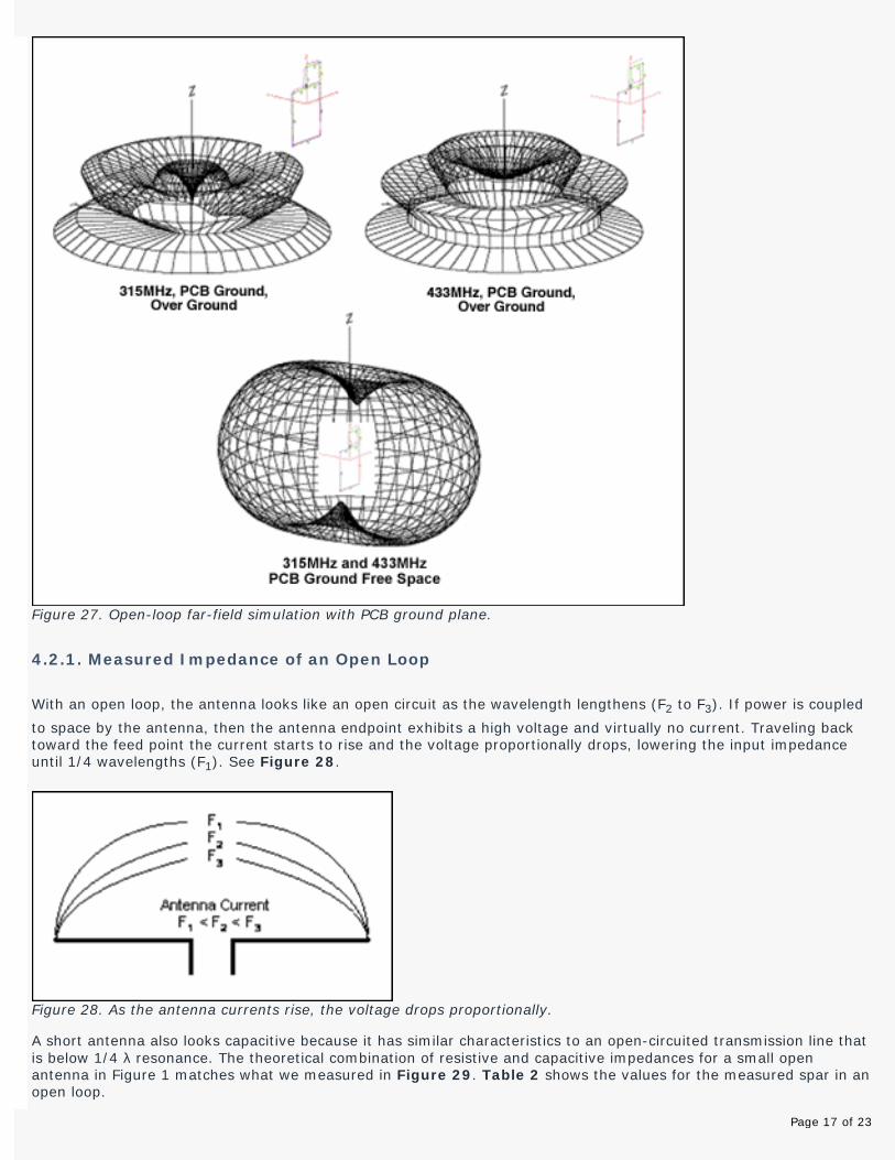
Figure 27. Open-loop far-field simulation with PCB ground plane.

4.2.1. Measured Impedance of an Open Loop

With an open loop, the antenna looks like an open circuit as the wavelength lengthens (F2 to F3). If power is coupled

to space by the antenna, then the antenna endpoint exhibits a high voltage and virtually no current. Traveling back toward the feed point the current starts to rise and the voltage proportionally drops, lowering the input impedance until 1/4 wavelengths (F1). See Figure 28.

Figure 28. As the antenna currents rise, the voltage drops proportionally. A short antenna also looks capacitive because it has similar characteristics to an open-circuited transmission line that is below 1/4 λ resonance. The theoretical combination of resistive and capacitive impedances for a small open antenna in Figure 1 matches what we measured in Figure 29. Table 2 shows the values for the measured spar in an open loop.

Page 17 of 23

Figure 29. Spar for open loop. Table 2. Measured Spar for a Shorted Loop Loop Antenna with Open End to Ground Plane

F (MHz) S11 mU Deg Re-Ω Im-Ω S11x S11y

330.00 982.360 -41.064 3.617 -133.41 0.741 -0.645

315.00 985.810 -38.054 3.359 -144.91 0.776 -0.608

330.00 982.360 -41.064 3.617 -133.41 0.741 -0.645

429.00 829.400 -97.517 8.191 -43.164 -0.109 -0.822

432.00 809.250 -101.860 8.682 -39.85 -0.166 -0.792

433.50 798.260 -104.200 8.940 -38.141 -0.196 -0.774

441.00 730.680 -118.520 10.441 -28.765 -0.349 -0.642

5. Spurious and Harmonic Antenna Considerations

The antenna of a transmitting device is typically the most influential and least understood component to the system performance. The antenna is, moreover, often severely compromised by the product's packaging requirements. Small devices that efficiently emit energy at a long wavelength relative to its size can also be very difficult to design even at UHF. Since the nth harmonics, by definition, will have shorter wavelengths by 1/n of the fundamental, the antenna can be a more efficient radiator to its harmonics than its fundamental. All coherent electromagnetic radiation that is propagated is subject to constructive and destructive interference when it is either reflected or converged by fields from another source. Radiating elements on a PCB are usually not only originating from one source, but typically the sum of many unintentional antennas caused by the fields coupling from the desired radiating element to associated components. To illustrate this effect, an example was created by using the antenna simulation program EZNEC. Figure 30 shows sources driving various elements at different phases (simulating active traces). These driven elements were then coupled to surrounding elements of random lengths (like leads, connectors, parts, screws, chains, traces, etc.), much like what is found on a PCB at 433MHz.

Page 18 of 23

Figure 30. Random element model simulated with the EZNEC software. From the far field, the simulation result at the fundamental shown in Figure 31 is very complex, even for just this simple model. In actuality, the effect of all the components on a PCB board would be impossible to simulate, which illustrates clearly the importance of field tests.

Figure 31. Fundamental PCB emissions from the simulated test results in Figure 29. Harmonics, by definition, will have shorter wavelengths, so their number of point sources and corresponding antenna efficiency increase. Since hardware inside an object is three-dimensional, the coupling and re-radiation of energy can also cause the harmonics to change polarization. Figure 32 below is an example of the same random element model shown in Figure 31, except at the second harmonic, 866MHz.

Page 19 of 23

Figure 32. Second harmonic of PCB emission. We extended the harmonics further to the 10th, and the far-field pattern became more complex with many strong discrete lobes. Notice also from Figure 33 that the spurious lobe along the Z axis grows and has substantially more antenna gain over the fundamental in the X-Y plane. Under such circumstances, the attenuation of spurious emissions and harmonics at the circuit level can be offset by gain from a more efficient radiator at higher frequencies. This results in undesired emissions that actually exceed the field strength of the fundamental.

Figure 33. Tenth harmonic of PCB emission. A polarization change could be caused by hardware that is perpendicular to the board like a 1/2 inch screw holding down a PCB of an antenna. If the PCB antenna is only 1 inch long and positioned vertically (X-Z axis) at 300MHz, it will, in fact, only be 19 electrical degrees long and thus both inefficient and vertically polarized. At the 40th harmonic, however, the screw mounted horizontally (along the Y axis) would be 190 degrees, a very efficient, nearly perfect dipole (Figure 34). If harmonics were rich in the transmitted signal, some of the energy can be coupled to the screw which results in a strong undesired, cross-polarized emission. In practice, one usually only has to worry about a few harmonics. The FCC will, nonetheless, require a device to meet emission limits well above 36GHz at all polarizations relative to the device.

Page 20 of 23

Figure 34. Ideal placement of the dipole screw in free space along the Y axis. Ground will also influence all emission dramatically. In free space the ideal radiator will look like a doughnut (Figure 34). If, however, the same radiator is placed three feet above ground or a reflecting surface, part of the main lobe in the -Z direction will bounce back and interfere with the main lobe in the +Z direction. Figure 35 shows the result, a floral pattern with a very strong lobe skywards and with the rising of the desired lobe in the lateral X-Y plane in the X direction.

Figure 35. Example of a dipole at 315MHz 3 feet above ground. Consider now a half-wave dipole oriented parallel to the ground and cut for each harmonic. The ground effect will diminish to some degree as the electrical length increases to ground. In practice, however, the fundamental radiator is a fixed length and will usually have more gain at its harmonic side lobes than the fundamental. The result is a complex interference of the lobes, as can be seen in Figure 36 below.

Page 21 of 23

Figure 36. Example of harmonics with a half-wave dipole cut at 300MHz, three feet above ground.

6. Summary

There is only one, truly accurate way to determine what elements are really radiated by an antenna. Careful measurements must be taken well beyond the fundamental radiated element, at all angles and polarizations to the device, and in the actual setting in which the transmitter is intended to be used. As frequency increases, shorted loops start out inductive and progress to resonance. Open loops, in contrast, start out capacitive and progress to their resonance. Both designs will have a small resistive component which is difficult to estimate through simulation or to measure, and which results in poor antenna efficiency. Field patterns for the open loop are normally more ground dependent due to the mirroring effects of the ground and tend to favor a dipole pattern. Shorted-loop elements, in contrast, have a large current component due to the short return to ground; the shorted loop is thus more like a magnetically coupled field which tends to approach a figure-8 pattern with less dependency to PCB ground. With small antennas, the efficiency and matching is better for the harmonics than the fundamental. Field patterns also become more complex as the current distribution varies across the element, thus resulting in interference patterns in the far field. Consequently, the harmonics for a small antenna are driven more efficiently, and the antenna itself can have unpredictable gain at undesired frequencies that are actually greater than the design frequency. The effect of the ground cannot be neglected. In practice, the ground has a very strong influence on both the measured result and the direction of the energy. While simulation accepts small loops, the value of simulation results is limited to gaining a general sense of how antennas work in an ideal environment and to understanding the effects of space and the ground. This general understanding can still be an especially useful insight, or an intuitive 'feel' for optimizing antenna results. References The theory of antennas and practical discussions can be found in these excellent sources:

Richard C. Johnson and Henry Jasik, Antenna Engineering Handbook, McGraw-Hill, 1961. RF Cafe, Smith Chart Generator (Fig. 3, 12, 18, and 25). Warren L. Stutzman and Gary A. Thiele, Antenna Theory and Design, John Wiley & Sons, Inc., 1981.

Page 22 of 23

Notes ¹Larry Burgess, "Matching RFIC Wireless Transmitters to Small Loop Antennas," High-Frequency Electronics, March 2005, pg. 24. ²Nittany Scientific. ³LLNL. 4Gerald Burke, Lawrence Livermore National Laboratory IPAC, "NEC Version 4.1," University of California, PO Box 808 L-795, 7000 East Ave, Livermore CA, 94559. 5WIPL-D. 6Cullen College of Engineering.

Application note 3621: www.maxim-ic.com/an3621 More Information For technical support: www.maxim-ic.com/support For samples: www.maxim-ic.com/samples Other questions and comments: www.maxim-ic.com/contact

Automatic Updates Would you like to be automatically notified when new application notes are published in your areas of interest? Sign up for EE-Mail™.

AN3621, AN 3621, APP3621, Appnote3621, Appnote 3621 Copyright © by Maxim Integrated Products Additional legal notices: www.maxim-ic.com/legal

Page 23 of 23