slusky... · web viewadditionally, the ratio of male to female live births decreases by 0.9...
TRANSCRIPT

The Impact of the Flint Water Crisis on Fertility
Daniel S. GrossmanDavid J.G. Slusky
March 7, 2018
Abstract
Flint changed its public water source in April 2014, increasing lead and other contaminant exposure. Exploiting variation in the timing of births we find fertility rates decreased by 12%, and overall health at birth decreased, compared to other cities in Michigan. Using a selection-scarring model, we find a net of selection scarring effect of 4.9% decrease in birth weight. These effects are likely lower bounds on the overall effects of this exposure due to long-term effects of in utero exposure. We apply an imperfect synthetic control model (Powell 2017), and expand on this method by including figures in our analysis.
Keywords: Women’s Health; Birth Rate; Fertility Rate; Birth Outcomes; Lead; Environmental Regulation; Michigan
JEL Codes: H75, I12, I18, J13, Q53, Q58
Affiliations:
Grossman (corresponding author): Department of Economics, West Virginia University, 1601 University Ave., 411 College of Business and Economics, Morgantown, WV 26506-6025; [email protected]
Slusky: Department of Economics, University of Kansas, 1460 Jayhawk Blvd., 415 Snow Hall, Lawrence, KS, 66045, [email protected]
Acknowledgements:
We thank Vincent Fransisco, Kate Lorenz, Matt Neidell, Dhaval Dave, Dietrich Earnhart, Josh Gottlieb, Ben Hansen, Shooshan Danagoulian, Scott Cunningham, Edson Severnini, David Keiser, Peter Christensen, Charles Pierce, Nicolas Ziebarth, Nigel Paneth, Tom Vogl, Nick Papageorge, seminar participants at the University of Minnesota, University of North Carolina, Appalachian State University, and Johns Hopkins University, and other conference participants at the 2017 iHEA conference, the 2017 National Bureau of Economic Research Summer Institute, and the 2017 APPAM Conference for all of their suggestions and feedback. We also thank Glenn Copeland of the Michigan Department of Community Health, Vital Records and Health Statistics Division for providing vital statistics data, the University of Michigan-Flint GIS Center for sharing data, David Powell for sharing his imperfect synthetic control method code, the West Virginia University Center for Free Enterprise for financial support, the Big XII Faculty Research Fellow Program, and the staff at KU IT for managing our research server.
1

“We were drinking contaminated water in a city that is literally in the middle of the Great Lakes, in the middle of the largest source of fresh water in the world. This corrosive, untreated water created a perfect storm for lead to leach out of our plumbing and into the bodies of our children.” - Dr. Mona Hanna-Attisha
1. Introduction
A recently released budget plan calls for extensive cuts to the EPA workforce and budget,
including compliance monitoring such as testing for lead and other water pollutants (Davis
2017).1 There is overwhelming evidence that lead in water contributes to higher rates of lead in
the blood, and is related to eventual developmental problems in children (Edwards,
Triantafyllidou, and Best 2009; Hanna-Attisha et al. 2016).
In this paper, we estimate the effect of the higher lead content of water sourced from the
Flint River on fertility and birth outcomes. Importantly, during the period in which water was
sourced from the Flint River (beginning on April 25, 2014), local and state officials continually
reassured residents that the water was safe. Officials did not issue a lead advisory until
September 2015, just a few weeks before switching off Flint River water for good (Fonger
2015a). This reduced the scope of an avoidance behavioral response to the water crisis (see e.g.
Neidell 2009).2 Flint had previously used the Flint River as its water source until 1967, switching
due to concerns about historic pollution from the dwindling auto industry. The state of Michigan
passed a law in 2000 expanding the state’s Department of Environmental Quality’s oversight
over the river. When the city switched back to it for their water source in 2014, many residents
and officials hoped cleanup efforts of the river had been successful (Carmody 2016).
1 The proposed cuts also entail curbing funding for the EPA Lead Renovation, Repair, and Painting Program.
2 When individuals change their behaviors in response to environmental or health information, the estimated effect contains both a biological and individual response, which are difficult for the econometrician to separate.
2

High lead content in the blood affects nearly all organ systems and is associated with
cardiovascular problems, high blood pressure, and developmental impairment affecting sexual
maturity and the nervous system (Agency for Toxic Substances and Disease Registry; Zhu et al.
2010). Recent studies have linked maternal lead exposure to fetal death, prenatal growth
abnormalities, reduced gestational period, and reduced birth weight (Edwards 2014; Zhu et al.
2010; Taylor, Golding, and Emond 2014); while historically lead is associated with increased
fetal death and infant mortality rates (Clay, Troesken, & Haines 2014), and the poisoning of
many adults as well (Troesken 2006). Maternal lead crosses the placenta providing a potential
direct link for lead poisoning of the fetus (Taylor, Golding, and Emond 2014, Lin et al. 1998).
In addition to increased lead content, the Flint water supply also contained higher rates of
bacteria including fecal coliform, trihalomethanes (TTHMs), among other contaminants.
Previous work has suggested that trihalomethances may be detrimental to pregnant women
(Gallagher et al. 1998, Nieuwenheijsen et al. 2000, Cao et al. 2016), although others dispute this
association (see e.g. Yang et al. 2007, Horton et al. 2011). The water change likely led to a
Legionnaires disease outbreak in Flint that killed as many as 12 individuals (Rhoads et al. 2017).
While we cannot separately identify the effects of these contaminants, we focus mostly on lead
because of the large literature linking lead to poor pregnancy outcomes and the specific results
we have from Flint showing elevated lead levels (Hanna-Attisha et al. 2016).
We leverage the fact that only the city of Flint switched its water source at this time,
while the rest of Michigan did not. These areas provide a natural control group for Flint in that
they are economically similar areas and, with the exception of the change in water supply,
followed similar trends in fertility and birth outcomes over this time period.
3

We use the universe of live births in Michigan from 2008 to 2015 to estimate the effect of
a change in the water supply in Flint on fertility and health. Our results suggest that women in
Flint following the water change had a general fertility rate (GFR) of approximately 7.5 live
births per 1,000 women aged 15-49 fewer than control women of the same age group, or a 12.0
percent decrease. Because the higher lead content of the new water supply was unknown at the
time, this decrease in GFR is likely a reflection of an increase in fetal deaths and miscarriages
and not a behavior change in sexual behavior related to conception like contraceptive use.
Additionally, the ratio of male to female live births decreases by 0.9 percentage points in Flint
compared to surrounding areas. Finally, we present suggestive evidence that behavioral changes
are unlikely to drive our results.
Estimates of birth outcomes are less precise and at times contradictory. Birth weight,
estimated gestational age, and in utero growth rate all decreased as a result of the water crisis,
but these results are small and not consistently statistically signficant. On the other hand,
abnormal conditions also decreased by approximately 13.4 percent in Flint following the water
switch compared to controls.3
Because of the large decrease in fertility rates, selection into birth is a major concern for
our birth outcome results. To account for this selected sample, we perform a bounding exercise
which provides an upward bound on the birth weight effect caused by the water change (Bozzoli,
Deaton, and Quintana-Domeque 2009). We find a nearly 5 percent decrease in birth weight. This
estimate fo the selection-scarring effect of in utero exposure to a contaminated water source is a
contribution to both the fetal origin literature and the health effects of lead literature.
3 Abnormal conditions include assisted ventilation, NICU admission, receipt of surfactant replacement therapy, antibiotic receipt to treat neonatal sepsis, seizure, and significant birth injury.
4
This study contributes to the large literature on fetal origins hypothesis. In his seminal
work, Almond (2006) discusses how in utero shocks may affect health. The sign of the effect of
these shocks is ambiguous due to two countervailing mechanisms. First, these shocks may lead
to “selective attrition,” or the culling of weaker fetuses through miscarriage or fetal death. Thus,
the less healthy fetuses would not be born, leaving only the healthier fetuses, or a potentially
positive effect on population health. Alternatively, although not mutually exclusively, higher
rates of lead may shift the overall health distribution of infants affected in utero. In this case, the
shift in the entire health distribution towards infants being more unhealthy would lead to worse
health outcomes for those affected by the shock. The two effects (selection and scarring) could
even approximately cancel each other out for surivors (Bozzoli, Deaton, and Quintana-Domeque
2009). For example, in the case of the Great Chinese Famine, taller children were more likely to
survive but then were stunted, resulting in a minimal change in height for the affected cohort but
their unscarred children being taller (Gørgens, Meng, and Vaithianathan 2012).
Given that it has only been a few years since the natural experiment in Flint, and because
of the potential long term effects of lead on cognitive development (e.g., see Aizer et al. 2018),
we cannot make any definitive statement about whether babies born represent individuals with a
higher future health stock compared to control cohorts or if latent health for this group is actually
worse. We can however estimate the selection effect by focusing on the birth rate, and
investigate infant health of the surviving children to estimate the magnitute of the offsetting
scarring effect on survivors.
In section 2 we describe the timeline of events around the Flint water changes. We
present a literature review of health conditions associated with lead in Section 3 and describe
potential mechanisms through which lead may affect health. Section 4 describes our data. We
5

present our empirical methods in section 5 and our results in section 6. In Section 7 we describe
numerous robustness checks and then discuss our results in Section 8. Section 9 concludes.
2. Background on Flint
Flint is an old manufacturing city and the birthplace of General Motors (GM) (Scorsone
and Bateson 2011). The city has been shedding residents for many years, with its contraction
coinciding with GM closing several plants in and around Flint.4
Through 1967, the city sourced its drinking water from the Flint River. In 1967, Flint
switched its water source away from the Flint River because of concerns about serving a growing
population (Carmody 2016). They signed a deal to receive Lake Huron water via pipeline from
the Detroit Water and Sewerage Department (DWSD).
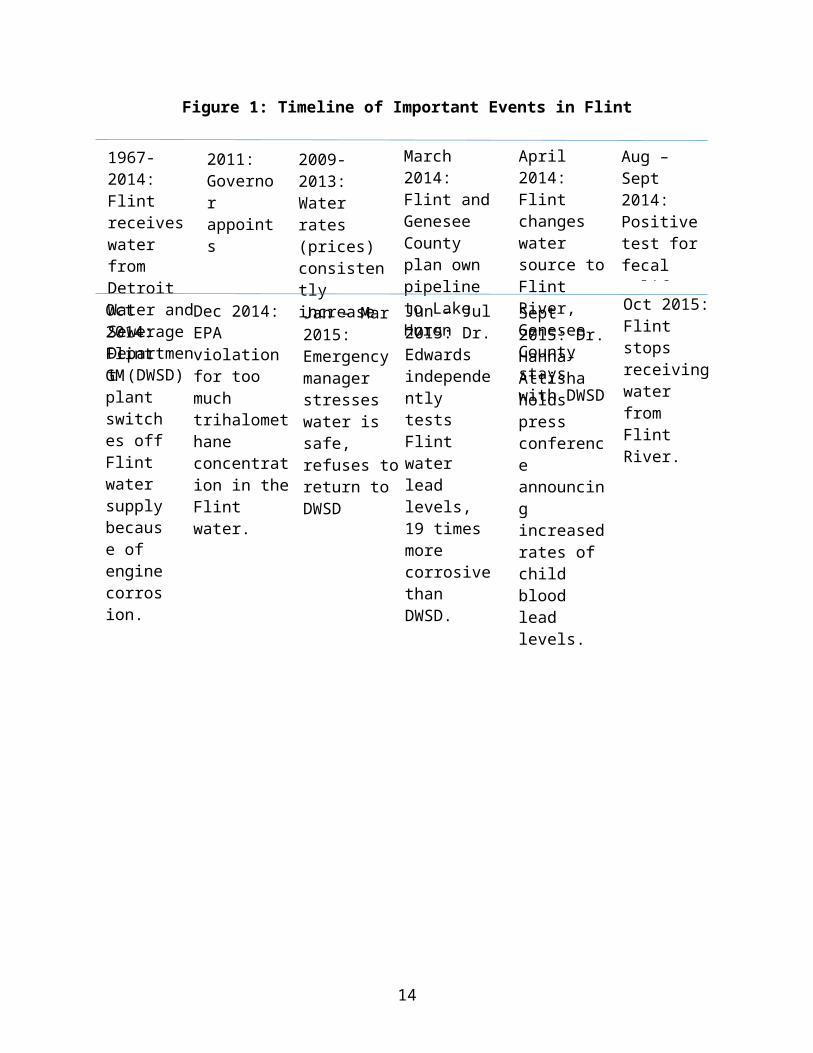
Figure 1 shows the timeline of events. In 2011 the Governor of Michigan installed an
Emergency Manager in the city who would make all fiscal decisions and “rule local
government,” based on the city’s precarious economic health (Longley 2011). This changed the
political economy of Flint and essentially meant that citizens and elected officials would have
little recourse to fight decisions made by the Emergency Manager. At the same time, DWSD
water rates were rising (Zahran, McElmurry, and Sadler 2017). To cut costs, the Emergency
Manager together with other Genesee County officials pursued a project to build a pipeline
directly to Lake Huron through the Karegnondi Water Authority (KWA) in March 2013 (City of
Flint 2015; Walsh 2014). This project would provide untreated water directly to Flint and the rest
of Genesee County upon its projected completion at the end of 2016, more than two years away.
When Flint announced this project, DWSD terminated the current agreeement, in place since
1967, to sell water to Flint but left open the possibility of a new agreement in the interim (Fonger
4 The number of inhabitants employed by GM decreased from 80,000 in 1978 to approximately 30,000 in the late 1990s to well under 10,000 today (Scorsone and Bateson 2011).
6

2013; Carmody 2016). Instead, Flint decided to use water from the Flint River to source its
drinking water between April 2014 and the completion of the KWA pipeline, while Genesee
County continued to receive water from DWSD.
Flint had to treat the new water source and while they used some of the same products as
the DWSD, like chlorine, they did not use anti-corrosive inhibitors such as orthophosphate
(Pieper et al. 2017, Olson et al. 2017). After switching to Flint River water, Flint citizens began
complaining about the color and smell of their water but were continually assured that the water
was safe to drink (City of Flint 2015a,b). The first sign of trouble came in August 2014 when a
boil advisory was announced for part of the city due to a positive fecal coliform test, although the
city minimized this adverse result claiming it was an “abnormal test” caused by a “sampling
error” (Fonger 2014a; Adams 2014). Less than a month later a second boil adivisory was
announced for a similar issue leading the city to increase chlorine levels in the water (Fonger
2014b). Then in October 2014, GM announced they would switch off of Flint River water in its
Flint plant because the water was too corrosive for its engine parts (Fonger 2014c). The city
confirmed the GM switch was best for engine parts but that the water was safe for human
consumption. In late December 2014, Flint received an EPA violation for excess trihalomethanes
(TTHM) in the water, likely caused by the chemicals used to treat the water (Fonger 2015b).5
Throughout early 2015, Flint held public meetings to assure citizens the water was safe
and that the TTHM violation would be fixed soon (City of Flint 2015a,b). During this time, the
Emergency Manager commissioned a report on the safety of the water and rebuffed an offer
5 Because of these additional contaminants found in Flint drinking water after the water switch, we cannot attribute all health effects to changes in lead. However, because of the well-established pathways through which lead effects health, including fetal health, described in more detail in the next section, we focus on lead in this paper. To the extent that these other contaminants are present in the water, our estimates would be an upper bound on the effect of lead on fertility and birth outcomes.
7

from DWSD to return Flint to Lake Huron water. A team from Virginia Tech, led by Mark
Edwards began independently testing Flint consumers’ water and in August 2015 reported much
higher levels of lead than previously reported, noting that Flint River water was many times
more corrosive than the DWSD water
(http://flintwaterstudy.org/wp-content/uploads/2015/10/Flint-Corrosion-Presentation-final.pdf).
Mona Hanna-Attish, a Flint pediatrician and researcher, held a press conference September 24,
2015 to report a substantial increase in blood lead levels in children following the water switch
(Fonger 2015c; Hanna-Attish et al. 2016). While the city initially attacked the results of this
study, the resulting public outcry finally led the city to switch back to Lake Huron water on
October 16, 2015 (Emery 2015). The crisis continues as those exposed to lead face potential life-
long problems.6 As of July 2017, the state Attorney General had filed indictments against 15
individuals for their roles in the Flint water crisis (Egan 2017).
6 https://www.washingtonpost.com/national/grant-to-create-registry-of-flint-residents-exposed-to-lead/2017/08/01/78c8fa66-7707-11e7-8c17-533c52b2f014_story.html?utm_term=.f89d3f64e273
8
Figure 1: Timeline of Important Events in Flint
9
1967- 2014: Flint receives water from Detroit Water and Sewerage Department (DWSD)
2011: Governor appoints Emergency Manager
2009-2013: Water rates (prices) consistently increase
March 2014: Flint and Genesee County plan own pipeline to Lake Huron
April 2014: Flint changes water source to Flint River, Genesee County stays with DWSD
Aug – Sept 2014: Positive test for fecal coliform, first boil advisory
Jan – Mar 2015: Emergency manager stresses water is safe, refuses to return to DWSD
Dec 2014: EPA violation for too much trihalomethane concentration in the Flint water.
Jun – Jul 2015: Dr. Edwards independently tests Flint water lead levels, 19 times more corrosive than DWSD.
Sept 2015: Dr. Hanna-Attisha holds press conference announcing increased rates of child blood lead levels.
Oct 2015: Flint stops receiving water from Flint River.
Oct 2014: Flint GM plant switches off Flint water supply because of engine corrosion.

3. Literature Review
3.1. Background on Lead
Lead is a heavy metal that is associated with health problems in children and adults. It
occurs naturally both in the earth’s crust and the environment. But, human activities, including
burning fossil fuels and other chemical reactions from industry, cause the majority of lead
emission into the environment (Agency for Toxic Substances and Disease Registry (ATSDR)
2007). The US banned lead paint in the 1970s and reduced leaded-gasoline throughout the 1980s
before banning it in 1996. These actions have decreased the incidence of lead emissions and the
concentration of lead in the blood dramatically over the past 40 years (CDC 2005, Zhu et al.
2010).
Exposure to lead is associated with many negative health and human capital outcomes.
Previous work has investigated the effects of general exposure to lead, lead levels in the blood,
and lead exposure from a water source on health and human capital. Additionally, it has explored
the mechanisms through which lead and other in utero exposure effects current and future health.
We discus each in turn below.
3.2. Exposure to lead
Exposure to lead is associated with cardiovascular problems, high blood pressure, and
developmental impairment affecting sexual maturity and the nervous system (ATSDR 2007; Zhu
et al. 2010). Lead crosses the placenta (Amaral et al. 2010, Schell et al. 2003, Rudge et al. 2009,
Lin et al. 1998) and is correlated with mental health issues, prenatal growth abnormalities,
reduced gestational period, and reduced birth weight (Hu et al. 2006; Zhu et al. 2010; Taylor,
Golding, and Emond 2014). Similarly, Clay, Portnykh, and Severnini (2017), using variation in
lead exposure from the introduction of the Interstate Highway System and the Clean Air Act,
10

find that exposure to lead in the air resulted in reductions in the birth rate and a worsening of
birth outcomes.
3.3. Lead Effects in Water
High lead content in water leads to increases in lead content in the blood (Edwards,
Triantafyllidou, and Best 2009; Hanna-Attischa et al. 2016), increasing the risk of the negative
health outcomes detailed above. Clay, Troesken, and Haines (2014) find historical evidence of
higher rates of fetal deaths in cities with more lead service pipes and more acidic water. Edwards
(2014) finds that fetal death rates increased and birth rates decreased following the increase of
lead in the water in Washington, DC from 2000 to 2003. While our paper is similar to that of
Edwards (2014), we use a substantially larger group of comparison cities to perform inference.
That study uses only Washington, DC compared to overall US and Baltimore, MD. This
comparison of just 2 areas makes proper inference difficult due to small clusters in both
treatment and control cities (see e.g. Cameron, Gelbach, and Miller 2008).
While previous studies have used exact measures of lead in the blood (see e.g. Taylor,
Golding, and Emond 2014; Zhu et al. 2010), these study designs do not include exogenous
variation in lead supply and thus cannot rule out that these worse birth outcomes are actually
associated with an omitted variable (or some other environmental factor that is associated with
both birth outcomes and lead concentration).
Beyond the change in water supply per se, lead increased in the Flint water supply
because of improper water treatment. Officials did not treat the Flint River water using corrosion
inhibitors, while simultaneously using ferric chloride (to combat infectious bacteria in the water)
which increased the likelihood of corrosion (Clark et al. 2015, Pieper, Tang, and Edwards 2017).
11
Corrosion inhibitors aid in creating protective corrosion scales within pipes, reducing the
amoung of lead leached from the pipes (Pieper, Tang, and Edwards 2017; Olson et al. 2017).
3.4. Other outcomes
Previous studies have found that changes in lead levels have a perverse effect on mental
health and criminality (Reyes 2007, 2015), educational outcomes (Aizer et al. 2018), and school
suspensions (Aizer and Currie 2017, Billings and Schnepel 2018). However, Billings and
Schnepel (2018) and Gazze (2016) find that lead remediation can moderate the negative effects
of those exposed to lead and reduce blood lead levels. Despite the overall positive effects of
remediation policies, for infants specifically Gazze (2016) finds a slight worsening of health
following state-level mandates designed to reduce exposure to lead paint.
3.5. Mechanisms
The change in the water source in Flint may affect health through several channels,
including selection into fertility, direct health effects, and indirect health effects. As discussed
above, fetal insults may reduce the overall fertility rate by reducing the number of viable fetuses
(Edwards 2014, Clay, Troesken, and Haines 2014). The expected direction of this effect on
overall health is ambiguous depending on which part of the fertility distribution it affects. If lead
only effects health by causing women to miscarry the weakest fetuses, we would expect the
remaining births to be healthier. However, if lead also shifts the health distribution of births then
we would expect either no change in overall health if selection and scarring effects perfectly
counterbalance each other or a decrease in health if the scarring effect dominates the selection
effect. Behavioral selection into pregnancy may occur if women decide not to get pregnant
because of worries about their future child’s health. Dehejia and Lleras-Muney (2005) document
non-random selection into pregnancy in response to changing labor market conditions while
12

Clay, Portnykh, and Severnini (2017) provide evidence of more educated women reducing
fertility in response to lead exposure. However, women would need to be aware of the water
crisis in advance for this explanation to affect our analysis. While women were aware of several
issues with Flint water following the change, they had no way of knowing about the lead content
in the water until nearly the end of the Flint River water regime (see Figure 3 below for support
of this). As noted, a general change in water quality may have made women less likely to
actively try to get pregnant regardless of lead knowledge. Additional figures similar to Figure 3
suggest this was not the case.
Lead may as well effect health through indirect channels including by decreasing latent
health of those infants carried to term. Latent health will be difficult to measure and may not
manifest until much later in life (Barker 1995; Schultz 2010; Almond and Currie 2011). Taken
together these studies suggest that exposure to lead in utero and in infancy may only represent a
lower bound on the overall effect of lead on health and human capital development.
4. Data
We use vital statistics data for the state of Michigan from 2008 to 2015. These data
contain detailed information on every birth in the state including health at birth and background
information on the mother and father which includes race, ethnicity, education, marital status, as
well as prenatal care and whether the mother smoked or drank alcohol during her pregnancy. We
calculate the date of conception for a woman from the clinical gestational estimate and exact date
of birth. We define Flint per the census tract-level (University of Michigan-Flint GIS Center
2017) data on lead pipes, and then use HUD census tract to ZIP code matching7 and SAS ZIP
code to city matching8 for the 15 largest non-Flint cities (i.e., Ann Arbor, Dearborn, Detroit,
7 https://www.huduser.gov/portal/datasets/usps_crosswalk.html#data
8 https://support.sas.com/downloads/download.htm?did=104285#
13
Farmington Hills, Grand Rapids, Kalamazoo, Lansing, Livonia, Rochester Hills, Southfield,
Sterling Heights, Troy, Warren, Westland, and Wyoming).9
Using population data from the American Community Survey10, we calculate general
fertility rate (GFR) as:
GFRct=12∗1000∗Total Birthsct
Population Aged 15−49ct (1)
where c indexes the city, and t the month and year. Total births are the exact number of births
occurring in the area for a given conception month, while population is a measure of the female
population of childbearing age.11 We multiply by 12 to make this an annual measure.
5. Methods
To assess the relationship between water source and fertility outcomes, we use a
difference-in-differences model to compare areas that received the new source to areas that did
not change their water source but were trending similarly in the pre-period. The difference-in-
differences model takes the form of the following:
Outcomect=a+β1Waterct +α c+δt +εct (2)
Where c indexes the city, and t the month and year. Outcome includes measures of GFR and
male to female sex ratio (sex ratio).12 GFR is a measure of the number of births conceived in a
9 In Appendix B, we compare Flint to the largest counties in Michigan and to all Michigan counties.
10 https://factfinder.census.gov/faces/tableservices/jsf/pages/productview.xhtml?pid=ACS_15_1YR_S0101&prodType=table – “State 040,” “Place 160”
11 Our analysis sample covers 95 months from May 2007 through March 2015. Because we use conception date, our 2008-2015 data contains complete date of conception data from approximately April 2007 through March 2015. We drop April 2007 data because the number of births from 2008 conceived in that month was substantially lower than all other 2007 months. This is likely due to births that occurred before 2008, which are not captured by our data set. 12 Our results are robust to using alternative specifications, including the natural log of the count of births and a nonlinear Poisson specification of the count of births. See Appendix Tables B3-
14

month given the total female population aged 15-49 of the city, as defined in equation (1) above,
and as shown below in Figure 2.
Figure 2: Comparison Cities
Note: Comparison cities are in blue, Flint in red, and cities with outlier GFR in green. Point size is proportional to the population of women age 15-49 in that city in 2014.
Water is a binary variable indicating whether the date of conception of the child occurred
after the water supply changed and whether the mother lived in Flint. We define being in utero
B4, and note that the coefficients are in log points, which for this range are approximately numerically the same as percentage points.
15
during the new water regime as a birth being conceived in November 2013 or later, which would
mean that at least one trimester of the pregnancy was affected by the water change. We include
city fixed effects, α c, to control for time-invariant characteristics of the city. δ t is a vector of
month and year fixed effects. City and time fixed effects subsume the main effects of living in
Flint and being in utero during the new water regime, respectively. We also investigate these
models using subsets of the data based on race, educational attainment, and age of mothers.
For birth outcomes, we estimate the following model:
Birthoutcomeict=a+β1Water ct+β2 X ict+γcen+δ t+εict (3)
where i indexes the individual, c the city, and t the month. Birthoutcome includes a binary
variable for any abnormal condition and a continuous variable for birth weight in grams,
estimated time of gestation in weeks, or fetal growth rate, defined as the birth weight divided by
weeks in gestation. Water is a binary variable indicating whether the date of conception of the
child occurred after the water supply changed and whether the mother lived in Flint. X ict is a
vector of variables capturing individual level socioeconomic characteristics of the mother and
child including gender of the child, race, ethnicity, marital status, and educational attainment of
the mother, which come from birth records. We include census tract fixed effects, γcen, to control
for time-invariant characteristics of the direct neighborhood of the mother. δ t is a vector of
month and year fixed effects, which control for seasonality of births and a general trend in birth
outcomes across Michigan over time. ε is an error term clustered at the city level.
The strengths of our study are that it exploits a natural experiment in the exposure of
women to contaminants, including lead, caused by an exogenous change in the water supply.
Any time a policy shift occurs that potentially causes an exogenous change, economists worry
about policy endogeneity, or the idea that this policy change occurred in response to conditions
16
that were already changing or in response to public pressure which would suggest additional
factors unobservable to the econometrician were present.
In this situation, the change we study is a change in the water supply for a municipality
that was decided by an unelected official, the Emergency Manager, appointed by the state
Governor.13 Furthemore, government officials continued to insist that the water was safe. An
EPA memo citing lead concerns was leaked to the public only in July, 2015, and confirmed by
other researchers in September, 2015 (Robbins 2016). Using Google Trends, in Figure 3 we
confirm an increase in concern about lead did not occur until September 2015, followed by a
large spike in searches in January 2016, when the national media began to pick up this story.
This likely greatly reduces the possibility of policy endogeneity in that the actual residents of the
municipality had little to no say in the matter and almost no recourse to make known any
displeasure they may have had with the change in water supply. We compare areas from the
same city and from adjacent counties who received water from the same supply source up until
the supply changed for Flint in April 2014. Conceivably, this change in water supply is the only
change that occurred at this time so any differences in fertility and birth outcomes between Flint
and similar counties over this time period can be attributed to the change in the water supply.
We additionally investigate several other keyword searches in google including TTHM,
trihalomethanes, water, water bottle, lead, pregnancy, baby, moving, escape, contraception,
abortion and find very little evidence of a change or spike in interest in any of these topics during
our period of interest.14
13 The water change was enacted to increase revenues in Flint and to reduce payments to the Detroit Water and Sewer Department while the city awaited the completion of a new pipeline (Fonger 2014d).
14 Importantly, the smallest Google trends data covers an area larger than just the city of Flint. While the exact boundaries are not published, it likely covers Genesee, Saginaw, and Bay Counties and likely also Midland County. As a robustness check we explore results using a
17

Figure 3: Google Trend Data on Searches for Water and Lead in Flint
Jan-0
4
Jan-0
5
Jan-0
6
Jan-0
7
Jan-0
8
Jan-0
9
Jan-1
0
Jan-1
1
Jan-1
2
Jan-1
3
Jan-1
4
Jan-1
5
Jan-1
6
Jan-1
70
10
20
30
40
50
60
70
80
90
100
Rela
tive
Sear
ch V
olum
e
Source: Google Trends
Notes: Searches for “flint water” in blue and “lead” in orange.
6. Results
Table 1 presents summary statistics of fertility rates and birth outcomes by time period in
Michigan. Columns (1) and (2) present means of births to individuals who did not reside in Flint
before and after the water change, respectively. Descriptive statistics for mothers who lived in
Flint at the time of birth before the water change are presented in Column (3) while results for
Flint mothers who gave birth after the water change are presented in Column (4). In general, we
consider a birth as occurring after the water change if the mother conceived in November 2013
or later.15
“treated” area of all of these four counties compared to other counties and still find a statistically significant, though attenuated result.15 This allows for a mother to be considered “treated” if she lived under the new water regime for at least one trimester of her pregnancy.
18
Mothers who gave birth outside of Flint were older (27.6 years compared to 24.7 years)
in the pre-period. However, we find no differential change in age between the periods. Women in
Flint also had lower educational attainment. They were much more likely not to have a high
school diploma and less likely to have obtained a college degree. While the proportion of
mothers who did not receive a high school diploma decreased by approximately 2.5 percentage
points for both Flint and non-Flint mothers following the water change, Flint mothers were more
likely to receive a high school diploma and non-Flint mothers were more likely to complete
some college or a college degree.
The general fertility rate in Flint was nearly 8.5 births per 1000 women aged 15-49 lower
in Flint following the water change compared to control areas. The sex ratio of babies born in
Flint skewed more female following the water change, a decrease of 0.74 percentage points.
Babies born in Flint were nearly 150 grams lighter than in other areas, were born ½ a week
earlier and gained 5 grams per week less than babies in other areas in the pre-period. The
unadjusted difference-in-differences for these variables was a decrease of 15 grams, 0.12 weeks
of gestational age and 0.27 grams per week in growth rate.
19

Table 1: Summary Statistics
(1) (2) (3) (4) (5)Non-Flint Births Flint Births
Pre-Water Change
(N=269,151)
Post-Water Change
(N=59,057)
Pre-Water Change
(N=10,623)
Post-Water Change
(N=2,010)
Difference in
DifferencesDemographic variables:
Mother’s age (years) 27.68(6.04)
28.27(5.75)
24.66(5.60)
25.17(5.37) -0.07
Mother no high school 0.177 0.145 0.294 0.271 0.010Mother high school grad 0.259 0.255 0.317 0.343 0.043***Mother some college 0.282 0.299 0.337 0.337 -0.021Mother college grad 0.272 0.290 0.050 0.047 -0.02***Outcome variables:
General fertility rate 67.09(5.01)
70.12(2.87)
62.28(6.81)
56.87(6.76) -8.45***
Male-Female Sex Ratio (percent male)
51.15(0.77)
51.04(1.24)
51.05(4.59)
50.20(3.06) -0.74
Abnormal Conditions 0.093(0.29)
0.110(0.31)
0.185(0.39)
0.177(0.38) -0.03***
Birth weight (grams) 3234(628)
3,209(641)
3,082(632)
3,042(651) -15
Estimated gestational age (weeks)
38.52(3.03)
38.39(2.54)
38.10(3.14)
37.89(2.69) -0.08
Gestational Growth (grams/week)
83.54(14.58)
83.03(14.51)
80.36(14.36)
79.58(14.48) -0.27
Notes: For Columns (1)-(4), standard deviation for non-dummy variables in parenthesis. For Column (5), robust standard errors are in parentheses. *** p<0.01, ** p<0.05, * p<0.1
20
6.1. Fertility Results
Figure 4: Unadjusted Monthly GFR16
Note: The vertical blue line is at November 2013, the first month in which all conceived births would have been affected by the water supply for at least one trimester.
In Figure 4 we present trends in GFR for Flint and the rest of Michigan separately. We
present unadjusted fertility rates.17 While births in Flint are still slightly more volatile due to the
16 This figure does appear to show city specific seasonality. Given the differences in the demographic composition of Flint and some other cities and the correlation between socioeconomic status and birth seasonality (Trivers and Willard 1973) we run a specification using city specific month fixed effects and find virtually identical results.
17 We calculated a 13 month moving average (+/- 6 months) to remove both seasonality and idiosyncratic noise in Appendix Figure B1.
21

smaller base sample in the area, the graph demonstrates a substantial decrease in fertility rates in
Flint for births conceived around November 2013, which persisted through the beginning of
2015. Flint switched its water source in April 2014, meaning these births would have been
exposed to this new water for a substantial period in utero (i.e., at least one trimester). Other
cities in Michigan had similarly seasonally volatile GFR trends, but did not display large
decreases in GFR following the Flint water switch.
Table 2: Lead in Water on General Fertility Rate
(1) (2) (3) (4) (5)
Water (β1¿ -7.451*** -7.451*** -7.451*** -7.451*** -5.682***(0.786) (0.791) (0.791) (0.811) (0.603)
[0.004]Conception Month Fixed Effects
X X X X
Conception Year Fixed Effects
X X X X
City Fixed Effects X X XConception Month into Year Fixed Effects
X X
City Linear Time Trends XObservations 1,520 1,520 1,520 1,520 1,520Cities 16 16 16 16 16R-squared 0.003 0.019 0.235 0.269 0.303Mean 62.28 62.28 62.28 62.28 62.28
Notes: Robust standard errors clustered at the city level in parentheses. Brackets contain wild bootstrapped p-values for the most saturated models. *** p<0.01, ** p<0.05, * p<0.1
Table 2 presents regression results for GFR by city. The main coefficient of interest is β1, the
parameter of Water ct calculated using equation (2) above. The unit of observation is city-month.
Column 1 does not include any covariates. We estimate that women living in Flint following the
water change gave birth to 7.5 fewer infants per 1,000 women aged 15-49 compared to control
counties. These results are statistically significant at the 0.001 (0.01%) level. This is on a base of
62 births per 1000 women aged 15-49, or a 12.0 percent decrease in births in Flint. In Column 2
22

we include conception month fixed effects and conception year fixed effects and in Column 3 we
additionally include city fixed effects in equation (2). In column 4 we include a more flexible
measure of time fixed effects by interacting month into year. Estimates are nearly identical in
these more saturated models. We adjust our standard errors using the wild bootstrap method
(Cameron, Gelbach, and Miller 2008) because we only have one treated cluster. We do include
city specific linear time trends in column 5, and the results are statistically significant, but we not
consider them our main results because of concerns about potentially biased treatment group-
specific time trends (Wolfers 2006, Lindo and Packham 2017)18
As an additional check, we perform a randomization inference permutation test,
following Cunningham and Shah (2018) and Fischer (1935). This test essentially systematically
assigns treatment status to each control area and compares the size of the implied treatment
effect for each control area to that of the actual treated area. We find our effect size in Flint is
larger than all control area “treatment effects” which suggests our inference above is indeed
correct. Figure 5 shows our treatment effect sizes for each city, with our Flint effect of -7.451 the
leftmost estimate.
In Table 3, we examine how the sex ratio of live births changed in Flint, given the
medical literature that male fetuses are more susceptible to fetal insults (Trivers and Willard
1973, Sanders and Stoecker 2015).
Figure 5: Randomization Inference Permutation Test
18 In an attempt to determine the share of the reduction in live births from fetal deaths, we sought to obtain administrative records on fetal deaths from the state of Michigan. Unfortunately, the state sent us two different data files which show different results, and so we are unable to report whether the fetal death rate increased or decreased. However, even using the data set that gives the largest increase in the fetal death rate only explains 2% of the decrease in the fertility rate.
23

02
Freq
uenc
y
-10 -5 0 5Average Treatment Effect
Flint Comparison cities
We find that sex ratios decrease by 0.9 percentage points (1.8 percent) in Flint, compared to
other Michigan cities. Sanders and Stoecker (2015), investigating the health effects of the Clean
Air Act, find that birth ratios skew more male following the implementation of the act. They
argue this is consistent with an increase in health. While this increase in the proportion of births
that are female likely represents a level of selection consistent with an increase in fetal deaths, it
is also consistent with a decrease in health at the time of birth. Again, given the concerns of
biased treatment group-specific time trends (Wolfers 2006, Lindo and Packham 2017), we are
not concern by the results in column 5 being far smaller in magnitude.
24
Table 3: Sex Ratios
(1) (2) (3) (4) (5)
Water (β1¿ -0.0092*** -0.0092***
-0.0092*** -0.0092*** -0.00121
(0.00260) (0.00262) (0.00262) (0.00268) (0.00411)[0.004]
Conception Month Fixed Effects
X X X X
Conception Year Fixed Effects
X X X X
City Fixed Effects X X XConception Month into Year Fixed Effects
X X
City Linear Time Trends XObservations 1,520 1,520 1,520 1,520 1,520Cities 16 16 16 16 16R-squared 0.003 0.019 0.235 0.269 0.303Mean 0.510 0.510 0.510 0.510 0.510
Notes: Robust standard errors clustered at the city level in parentheses. Brackets contain wild bootstrapped p-values for the most saturated models. *** p<0.01, ** p<0.05, * p<0.1
6.1.1. Sub-Sample Analyses
Given the large decreases in general fertility rates and the shift towards more female
births we find for Flint overall, in this next section we investigate whether these results hold over
all time periods and all individuals in Flint by limiting our analysis sample.
In Table 4, we present our main results as well as results limiting our sample to general
fertility rates of births conceived before September 2014 and dropping the cities with the highest
and lowest GFRs. We investigate births conceived before September 2014 because of potential
avoidance given boil advisories due to fecal coliform in the Flint water source reported around
this time. The decrease in fertility rates was actually larger in this early period, with Flint’s GFR
nearly 9 births per 1000 women aged 15-49 lower than other cities’ GFR following the water
change. One potential explanation for this change is that avoidance behaviors led Flint residents
25

to begin buying bottled water at higher rates after September 2014 (Christensen, Keiser, and
Lade 2017).19 Additionally, when we omit the cities with the highest and lowest GFR in the
sample and compare GFR in Flint to the remaining 13 largest cities in Michigan, we find a
reduction in GFR of 8 births per 1000 women in Flint following the water change. This is of a
very similar magnitude to our main results.
Table 4: Lead in Water on General Fertility Rate, Sample Changes
(1) (2) (3) (4) (5)
Main Results (N=1520) -7.451*** -7.451*** -7.451*** -7.451*** -5.682***(0.786) (0.791) (0.791) (0.811) (0.603)
[0.004]Before 9/2014 (N=1424) -8.797*** -8.797*** -8.797*** -8.797*** -6.900***
(0.690) (0.695) (0.694) (0.712) (0.585)[0.004]
Drop Outlier Cities (cities=14, -8.173*** -8.173*** -8.173*** -8.173*** -5.549***N=1330) (0.693) (0.698) (0.697) (0.718) (0.678)
[0.004]Conception Month Fixed Effects
X X X X
Conception Year Fixed Effects
X X X X
City Fixed Effects X X XConception Month into Year Fixed Effects
X X
City Linear Time Trends X
Notes: Robust standard errors clustered at the city level in parentheses. Brackets contain wild bootstrapped p-values for the most saturated models. *** p<0.01, ** p<0.05, * p<0.1
In Table 5, we limit our sample to demographic subgroups. For this analysis we use
Poisson regressions because we cannot calculate annual measures of women between the ages 15
19 Additionally, our final time period, March 2015 shows a large increase in GFR for Flint, from which we are unable to determine if that month GFR is an outlier or a general trend towards higher GFRs.
26

and 49 in a given city.20 These analyses assume a constant population. First, for the sample as a
whole, we find a decrease of 0.151 which can be interpreted as a 15 percent decrease in births in
Flint following the water change. This is slightly larger than the 12 percent decrease we find in
Table 2 using GFR. Assuming an unchanging population likely explains this larger magnitude.
When we break our results down by race we find a similar 14 and 13 percent decrease for white
and black mothers, respectively.21 Results by education suggest that the decrease in births is
concentrated among the somewhat more educated mothers, with those with some college
decreasing births by 22 percent and those with a college degree decreasing births by 33 percent.
However, those with some college behave differently from those with a college degree,
suggesting they are not necessarily a convex combination of college graduates and only high
school graduates. For example, many of them had to drop out college due to a financial or health
shock or other family emergency, making them more economically disadvantaged than those
with no college even though they have more education (Pollak and Lundberg 2014).
Furthermore, the college graduate group in Flint is particularly small, less than 100 total
births post water change and thus readers should be careful not to ascribe too much weight to
these results as small variations may substantially affect our results. Lastly, estimates by age
groups show decreases in births across the spectrum, with the largest effect a 15 percent decrease
for mothers between the ages 25 and 34. Births to mothers aged 15 to 24 decreased 7 percent
while births to mothers aged 35 to 49 decreased 10 percent. Overall these effect sizes suggest a
fairly large effect across the population, with the exception of mothers with less education.
20 To calculate demographic subgroup specific populations we would have to rely on 5-year moving averages from the ACS, which given the short time period of the water switch would be very similar to the assumptions of the Poisson model of a constant population size.
21 We do not include wild bootstrap standard errors in these analyses because these are Poisson regressions.
27

Table 5: Lead in Water on General Fertility Rate, Subsample Analyses
(1) (2) (3) (4) (5)
All -0.151*** -0.151*** -0.151*** -0.151*** -0.151***(0.0166) (0.0166) (0.0166) (0.0166) (0.0166)
White -0.140*** -0.140*** -0.140*** -0.140*** -0.0804***(0.0172) (0.0172) (0.0172) (0.0172) (0.0262)
Black -0.119*** -0.119*** -0.125*** -0.125*** -0.0180(0.0172) (0.0173) (0.0164) (0.0164) (0.0177)
Less than High School -0.0520 -0.0525 -0.0397 -0.0397 0.0154(0.0448) (0.0447) (0.0450) (0.0450) (0.0369)
High School Only -0.0442 -0.0442 -0.0442 -0.0442 0.122***(0.0270) (0.0270) (0.0270) (0.0270) (0.0416)
Some College -0.215*** -0.215*** -0.215*** -0.215*** -0.224***(0.0144) (0.0144) (0.0144) (0.0144) (0.0216)
College Plus -0.328*** -0.328*** -0.328*** -0.328*** -0.00164(0.0192) (0.0192) (0.0192) (0.0192) (0.0118)
Age 15-24 -0.0683*** -0.0683***
-0.0688*** -0.0688*** -0.0629***
(0.00720) (0.00719) (0.00717) (0.00717) (0.0119)Age 25-34 -0.148*** -0.148*** -0.148*** -0.148*** 0.0244
(0.00806) (0.00806) (0.00806) (0.00806) (0.0244)Age 35-49 -0.101*** -0.101*** -0.101*** -0.101*** 0.0669***
(0.0212) (0.0212) (0.0212) (0.0212) (0.0188)Conception Month Fixed Effects
X X X X
Conception Year Fixed Effects
X X X X
City Fixed Effects X X XConception Month into Year Fixed Effects
X X
City Linear Time Trends X
Notes: N=1520 observations across 16 cities for all regressions. Robust standard errors clustered at the city level in parentheses. *** p<0.01, ** p<0.05, * p<0.1
28

Table 6: Sex Ratio, Sample Changes
(1) (2) (3) (4) (5)
Main Results (N=1520) -0.0092*** -0.0092***
-0.0092*** -0.0092*** -0.00121
(0.00260) (0.00262) (0.00262) (0.00268) (0.00411)[0.004]
Before 9/2014 (N=1424) -0.00231 -0.00231 -0.00231 -0.00231 0.00447(0.00291) (0.00292) (0.00292) (0.00300) (0.00445)
[0.468]Drop Outlier Cities (cities=14, -0.00898** -
0.00898**-0.00898** -0.00898** -0.00352
N=1330) (0.00299) (0.00301) (0.00301) (0.00310) (0.00409)[0.012]
Conception Month Fixed Effects
X X X X
Conception Year Fixed Effects
X X X X
City Fixed Effects X X XConception Month into Year Fixed Effects
X X
City Linear Time Trends X
Notes: Robust standard errors clustered at the city level in parentheses. Brackets contain wild bootstrapped p-values for the most saturated models. *** p<0.01, ** p<0.05, * p<0.1
We investigate changes in sex ratio for those conceived before September 2014 and
dropping cities with highest and lowest GFR in Table 6. We find that births conceived early in
the new water regime did not differ on sex ratios compared to other cities. However, when we
remove outlier cities, we find a near identical coefficient estimate to our main analysis.
In Table 7, we do a subsample analysis of the effect of the water change on sex ratios.
White mothers see a decrease in the ratio of female babies, while black mothers see an opposite
effect. The results by education are consistent with the fertility results above, with large
decreases in the ratio of female births for mothers with some college and a college degree. These
results suggest that if this is an avoidance story for these mothers, the mothers of this education
level who do give birth are a selected sample that differs from similarly educated mothers who
29

gave birth in Flint before the water switch in unobservable ways. Results by age are strongest for
those aged 25 to 34 and 35 to 49, which is consistent with our fertility results.
Table 7: Sex Ratio, Subsample Analyses
(1) (2) (3) (4) (5)
All -0.0092*** -0.0092***
-0.0092*** -0.0092*** -0.00121
(0.00260) (0.00262) (0.00262) (0.00268) (0.00411)White -0.0111*** -
0.0111***-0.0111*** -0.0111*** -0.00657
(0.00346) (0.00348) (0.00348) (0.00357) (0.00661)Black 0.0182* 0.0182* 0.0182* 0.0181* 0.0249
(0.00939) (0.00943) (0.00943) (0.00978) (0.0169)Less than High School -0.00178 -0.00178 -0.00220 -0.00236 0.0299*
(0.0148) (0.0148) (0.0149) (0.0152) (0.0173)High School Only 0.00210 0.00210 0.00210 0.00210 -0.00161
(0.00704) (0.00707) (0.00707) (0.00721) (0.00873)Some College -0.0252*** -
0.0252***-0.0252*** -0.0252*** -0.0265***
(0.00539) (0.00541) (0.00541) (0.00552) (0.00815)College Plus -0.0346*** -
0.0346***-0.0346*** -0.0346*** -0.0943***
(0.00741) (0.00745) (0.00745) (0.00759) (0.00955)Age 15-24 0.0112 0.0112 0.0111 0.0112 -0.00214
(0.00766) (0.00769) (0.00770) (0.00784) (0.0157)Age 25-34 -0.0238*** -
0.0238***-0.0238*** -0.0238*** -0.000642
(0.00447) (0.00449) (0.00449) (0.00457) (0.00531)Age 35-49 -0.0344*** -
0.0344***-0.0344*** -0.0344*** -0.0374***
(0.00462) (0.00465) (0.00464) (0.00473) (0.00957)Conception Month Fixed Effects
X X X X
Conception Year Fixed Effects
X X X X
City Fixed Effects X X XConception Month into Year Fixed Effects
X X
City Linear Time Trends X
Notes: N=1520 observations across 16 cities for all regressions. Robust standard errors clustered at the city level in parentheses. *** p<0.01, ** p<0.05, * p<0.1
30

6.2. Birth Outcomes
The results in the section above provide direct support for the Flint water change causing
a culling of the weakest fetuses. Next, we turn our focus to birth outcomes. If increased lead in
the water only has a selective attrition effect then we would expect an increase in health among
the births in Flint as the selection would remove only the weakest and leave the healthier fetuses
to come to term. If, alternatively, a scarring effect also is present, then we would expect a
decrease in health for those births that actually occurred. Lastly, if more educated women were
exhibiting avoidance behavior we would expect overall health to decrease due to this selective
sample.
We first investigate whether the change in water supply caused a change in abnormal
conditions in Table 8.22 Abnormal conditions decrease by 2.5 percentage points (13.5 percent) in
Flint compared to the rest of Michigan after the switch to Flint River water, a positive health
outcome. This result is statistically significant, although it is partially driven by the substantial
increase in abnormal conditions in other areas, which is unlikely to be attributable to the Flint
water change. Adding census tract, month and year of conception fixed effects and additional
covariates in columns 2-5 does not substantially change the coefficient on abnormal conditions.
Results for birth weight, gestational age and gestational growth rate are all negative but
imprecisely measured. The magnitudes on the coefficients are all rather small, suggesting non-
economically meaningful effect sizes. For birth weight, we find the water change decreased birth
weight by between 12 and 22 grams. None of these estimates is statistically significant.
Estimates of the effect of the water change on estimated weeks of gestation suggest that babies
born in Flint after the water change were in utero for 0.1 weeks less than before the change
22 Abnormal conditions include assisted ventilation, NICU admission, receipt of surfactant replacement therapy, antibiotic receipt to treat neonatal sepsis, seizure, and significant birth injury.
31

compared to the rest of Michigan. This amounts to a reduction of less than 1 day in utero.
Growth rate is calculated as an infant’s birth weight divided by his or her gestational age. We
find that those born in Flint after the water switch grew between 0.3 and 0.4 grams per week less.
Table 8: Lead in Water on Other Birth Outcomes
(1) (2) (3) (4) (5)
Abnormal Conditions -0.0254*** -0.0237** -0.0236** -0.0234** -0.0249**(0.00970) (0.00970) (0.00968) (0.00968) (0.00970)
Birth weight (grams) -15.24 -21.51 -20.21 -19.02 -11.52(13.61) (14.62) (14.44) (14.74) (14.59)
Gestational Age (weeks) -0.0790 -0.102* -0.0885 -0.0892 -0.0765(0.0591) (0.0618) (0.0601) (0.0599) (0.0601)
Gestational Growth -0.271 -0.400 -0.381 -0.349 -0.173(grams/week) (0.306) (0.327) (0.324) (0.333) (0.331)
Census Tract Fixed Effects X X X XConception Month Fixed Effects
X X X
Conception Year Fixed Effects
X X X
Child Sex Control X XMom Controls XN 340,841 340,841 340,841 340,841 340,841
Notes: Robust standard errors clustered at the census tract level in parentheses. *** p<0.01, ** p<0.05, * p<0.1
6.3. Behavioral Changes
One possible concern with lower conception rates having a role is that they are a result
of behavioral changes (i.e., less sex) and not the physiological impacts of lead. Following
Barreca, Deschenes, and Guldi (2016) we use the American Time Use Survey to investigate time
spent engaged in sexual relations, proxied by any time spent in “personal or private activities”.23
23 I.e., “having sex, private activity (unspecified), making out, personal activity (unspecified), cuddling partner in bed, spouse gave me a massage.”
32

Table 9 has the result of those analyses. Note that these analyses are at the county or CBSA-level
and are thus not directly comparable to our main results as Flint comprises approximately ¼ of
the population of Genesee County. Appendix Table B4 provides our main results treating all of
Genesee County as treated, which should bias our results towards zero.
Table 9: Time Use Data on Sex
(1) (2) (3) (4) (5) (6)County-level CBSA-level
Water (β1¿ 0.0148*** 0.0158*** 0.0157*** 0.0186*** 0.0206*** 0.0205***(0.00203) (0.00133) (0.00131) (0.00229) (0.00319) (0.00310)
Conception Month Fixed Effects X X X
Conception Year Fixed Effects X X X X
County Fixed Effects X
CBSA Fixed Effects X
Observations 861 861 861 745 745 745Counties/CBSAs 16 16 16 13 13 13R-squared 0.011 0.037 0.036 0.003 0.028 0.027
Notes: Robust standard errors clustered at the county or CBSA level in parentheses. *** p<0.01, ** p<0.05, * p<0.1
We find that sexual activity increased in the post period, which would bias our main result of a
decrease in the fertility rate toward zero.24 While this is only suggestive evidence, it supports our
conclusion that the reduction in the conception rate is not driven by a reduction in sexual
activity.25
24 This is analogous to Barreca, Deschenes, and Guldi (2016) which also finds a statistically significant increase in time in the probability that individuals spend time on sex during environmental conditions that overall reduce fertility.
25 As an extension of the CPS, the ATUS lacks city identifiers and only has county or CBSA ones. In Appendix Table B4, we repeat our results are the county level and show that while the inclusion of the rest of Genesee County (where Flint is located) as treated reduces the magnitude of our results, they are still directionally consistent and statistically significant in some specifications.
33

6.4. Synthetic Control Methods
Lastly, we perform an analysis of fertility rates using a synthetic control methods
approach (Abadie and Gardeazabal 2003; Abadie, Diamond, and Hainmueller 2010;
Cunningham and Shah 2018).26 This method creates a weighted matched control group that more
closely resembles the characteristics of Flint in the period before the water change on both level
and trend of fertility rates. It also controls for demographic characteristics of mothers in the pre-
period, including race/ethnicity, educational attainment, and gender of the child. Figure 6
presents the results of this method. Panel A displays GFR trends in Flint and its synthetic control
group before and after the water switch, which is visualized as the vertical line at November,
2013, which is the last conception date for which women would have been exposed for at least
one trimester to the new water supply.27 Panel B shows the difference between each city
systematically assigned to treatment and the synthetic version of the city for each month. Flint is
denoted by the solid line. The average treatment effect in Flint compared to the synthetic control
is a decrease of 11.6 births, presented in Panel C by the (blue bar) horizontal blue line. This
effect size is slightly larger than that found above in Table 2. The average treatment effect in
Flint is substantially larger than the average treatment effect for all other cities.28
As an additional robustness check, we perform a synthetic control model matching on all
GFR for the month of March in each year before the water change (2008, 2009, 2010, 2011,
26 We describe this method in detail in Appendix A.
27 We find similar effect sizes and inference interpretations using quarter of birth rather than month of birth (results available upon request).
28 We perform a similar analysis dropping outlier cities, e.g. the city in Figure 6, Panel B which is clearly well above all other estimates and present these results in Panel D. We also perform an analysis dropping Flint from the inference analysis so that when we assign treatment to each control group, Flint cannot be used as a synthetic control. These do not change our results.
34

2012, 2013).29 The strength of this analysis is that it creates a better pre trend match on GFR, but
the weakness is that it may over-fit on GFR and ignore other covariates (see Kaul et al. 2017).
Our estimates are robust to this alternative specification and we present these results in Appendix
Figure B3.30
Finally, because our pre-trend match may be imperfect which would affect our inference,
we use an imperfect synthetic control method (Powell 2017), which we believe we are the first to
use aside from Powell’s own demonstrations, and the first to include figures as part of the
method. This method solves two issues in the Abadie et al. (2010) method. First of all, it
improves inconsistent pre-period match due to transitory shocks by using pre-period outcomes
predicted from city-specific flexible time trends, instead of the actual per-period outcomes.
Secondly, it allows for treated group being an outlier by using treated group’s presence in other
group’s synthetic controls. More specifically, an outlier treated group cannot match the outcomes
of a convex combination (i.g., with nonnegative weights) of the control units. But a convex
combination of the treated group and the rest of the control group could match the outcome of
control group that has been assigned a placebo treatment. If the treated group has a positive
weight in this situation, that weight can be inverted to describe the mapping from the control
group to the treated group.
These two fixes reduce bias in the estimates and out performs the synthetic control
method in simulations (Powell 2017). In Figure 7, Panel A shows that the new imperfect
synthetic control group is a better match for Flint in the pre-period. Panel B demonstrates that the
29 We estimate a similar model matching on the 4th quarter GFR for each year before the water change (2007, 2008, 2009, 2010, 2011, 2012) and find comparable results (Available upon request).
30 We also perform similar synthetic control analyses using a 13 month moving average for GFR (as described above) and find quantitatively and qualitatively similar results.
35

decrease in GFR in Flint is larger than in any other area following the water change which
provides additional evidence of the statistical significance of our estimates.
Figure 6: Synthetic Control Results for General Fertility Rates
Panel A. Flint GFR compared to Synthetic Panel B. Difference Between Each City Flint GFR and it’s Synthetic Counterpart
Panel C. Inference using Average Treatment Panel D. Dropping outlier (same as Effect panel b above without Wyoming, Michigan)
Note: The blue vertical line in Panel A is at November 2013, which is the last conception date for which women would have been exposed for at least one trimester to the new water supply. The blue solid line in Panel B represents the difference between GFR in Flint and “synthetic Flint.” The blue bar in Panel C displays the average treatment effect (ATE) for Flint, while red bars show comparison city ATEs. It is the most negative ATE compared to assigning all areas to treatment, suggesting statistical significance.
36
Figure 7: Imperfect Synthetic Controls
Panel A. Flint GFR compared to Imperfect Panel B. Inference using Average Treatment Synthetic Flint GFR Effect
4050
6070
80G
FR
0 20 40 60 80 100Months
Flint Synthetic Control
02
Freq
uenc
y
-10 -5 0 5 10Average Treatment Effect
Flint Comparison cities
Note: The blue vertical line in Panel A is at November 2013, which is the last conception date for which women would have been exposed for at least one trimester to the new water supply. The blue bar in Panel B displays the average treatment effect (ATE) for Flint, while red bars show comparison city ATEs. It is the most negative ATE compared to assigning all areas to treatment, suggesting statistical significance.
7. Robustness Checks
We perform a number of robustness checks to ensure our results are not sensitive to
geographical definitions of our control group or of Flint, or functional form assumptions. In
Appendix Table B1 we estimate the effect of the water change on log births. We find between a
15 and 18 percent decrease in Flint following the water change, which is comparable to our 12 to
14 percent result in Table 2. In Appendix Table B2 we estimate a Poisson model and find a
decrease in births of 0.15, which can be interpreted as similar to a 15 percent decrease in births in
Flint. These results assume a constant population in Flint over the study period. Estimates of
population in Flint decrease over the study period which may partially explain the larger
magnitude of the effect in log and Poisson models.
We compare county level GFR rates in Appendix Table B3. The treatment in this table
includes all of Genesee County, of which Flint comprises approximately ¼ of the population.
37

The results are greatly reduced in this table, which is to be expected given that the treatment
sample is contaminated with non-affected areas. However, GFR still decreases in a statistically
significant way in Genesee County compared to other counties in Michigan following the Flint
water change.31
As a placebo analysis, we compare Genesee County, excluding Flint, to the rest of
Michigan in Appendix Table B5 and find no change in GFR or sex ratios providing strong
support for a change within Flint at the time of the water switch driving our results.
In Appendix C, we focus on Flint compared to counties in Michigan rather than cities.
The results are largely robust to this alternative definition of control areas. The main difference
between these results and our main city comparison results are that the effect of the water switch
on fertility rates in Flint is slightly smaller than our main results, but birth outcome results are
slightly larger. The magnitudes of these differences are still quite similar. However, because
Flint is a city within a county and urban areas tend to have higher fertility rates, as is evidenced
in Appendix Figure B1, we focus on the city results and simply state that our results are robust to
other comparison groups.
31 With the exception of the county-specific linear time trend, which biases the results for the reasons described above.
38

8. Discussion
First of all, our results for the decrease in the fertility rate are plausible given the broader
scientific literature on this topic. While the impact of drinking water with high concentrations of
lead on fertility rates has not been studied in the economics literature, there has been some work
in the environmental science literature. Specifically, Edwards (2014) studies an increase in lead
in drinking water in Washington, D.C. in the early 2000s, and using somewhat different methods
finds a 12% decrease in the fertility rate. The magnitude of the fertility rate decrease that we
find is identical to Edwards’s result.
Secondly, we attempt to extrapolate the consequences of our results. The population of
women aged 15-49 in Flint during our study period is approximately 26,000. The GFR dropped
from 62 to 57, suggesting that over our study window of 17 months (births conceived from
November 2013 through March 2015) between 198 and 276 more children would have been born
had Flint not enacted the switch in water.32 We consider this strong empirical support for the
existence of a culling effect caused by increased lead in the water.33 Our results on sex ratios
suggest that among the live births that occurred in Flint following the change in water supply, an
additional 18 female infants were born than expected.34 While birth outcome results are not as
definitive as our fertility results, they provide evidence that the effect we find is likely a
combination of a selection and a scarring effect. In fact, even an effect size of zero for these birth
outcomes provides evidence of scarring because had there only been a selection effect, we would
32 We calculate this as the either the change in GFR in Flint only (62-57) or the difference-in-differences estimate (7.5) * population aged 15-49 in Flint (26,000) * the number of years affected (17/12) which gives us a range of 198 to 276.
33 Using log births instead of GFR provides consistent results, as shown in Appendix Table B1.
34 We multiply the change in sex ratio (0.009) * the number of post water change births (2,010) to get 18.
39

expect the health effects to be positive. Because we find evidence of negative health effects in
Flint following the water change, we conclude that in addition to reducing the number of
expected births in the city, the water change also caused a decrease in overall health of those
babies born.
We perform an analysis in the spirit of Bozzoli, Deaton, and Quintana-Domeque (2009)
to untangle scarring and selection. First, we assume that the pre-water change birth weight
distibriution in Flint is normally distributed (see Figure 8) and has the mean (3082 g) and
standard deviation (632 g) as in column 3 of Table 1. Using the 12.0 percent reduction in the live
birth rate as found in Table 2, we assume that this reduction all came from the left tail of the
birth weight distribution, as birth weight is often thought of as a proxy for infant health. Another
way to think of this is that there is some minimal birth weight cutoff for live birth, and the
selection shock of adding lead to the water shifted the entire distribution left such that the bottom
12.0 percent of birth weight did not survive.
Figure 8: Probability Density Function of Birth Weight Before and After the Water Switch.
40
0.0
002
.000
4.0
006
.000
8D
ensi
ty
0 2000 4000 6000 8000grams
Flint Pre-Water Flint Post-WaterNon-Flint Pre-Water Non-Flint Post-Water
Using the standard formula for the mean of a truncated normal35 we calculate that mean
birth weight of the surviving newborns, without any scarring, would have been 3242 g. From
here to the observed Flint mean birth weight in the post period (3042 g) is a decrease of 183 g.
Removing the pre-post difference in the rest of Michigan (from Columns 1 and 2 of Table 1)
reduces this by 25 g to a scarring effect of 158 g, which is a 4.9 percent decrease. This is much
larger than the scarring effect found from ignoring how scarring and selection cancel each other
out (as in Gørgens, Meng, and Vaithianathan 2012) and naïvely using the coefficient in Table 8.
We consider this a bounding exercise for the full effect of scarring had no selective attrition
occurred. As Figure 8 makes clear, despite the large amount of selective attrition we document in
Table 2, our pdf for Flint show that the health distribution shifted to the left in Flint following the
35 I.e., E (X|X>μ+σ Φ−1 ( p ))=μ+σϕ (Φ−1 ( p ) )
1−p, where μ is the mean, σ the standard deviation, Φ
the standard normal CDF, φ the standard normal PDF, and p the truncation cutoff probability.
41

water change and did not shift in comparison cities.
Additionally, while the results in Tables 3 and 5 are not definitive, taken together, they
also support our main result that fertility rates decrease because of both selective attrition and
scarring from a biological effect of an increase in contaminants including lead in the water. The
0.9 percentage point increase (1.8%) in female births following the water change, as shown in
Table 3, is consistent with medical literature (Trivers and Willard 1973). Sanders and Stoecker
(2015) find that an increase in particulates in the air reduces the ratio of male births.
Additionally, in Table 9, we find no evidence to support a decrease in sexual relations among
individuals living in Flint during this time period. For our results to be explained by behavioral
changes, we would have to postulate a theory that at the same time Flint changed its water
source, parents changed their preference for male children and began performing sex-selective
abortions showing a preference for female children. This result would run counter to the
prevailing evidence of lower female births than expected, especially in Asian countries (see e.g.
Sen 1990; Das Gupta 2005), but also in the US (Abrevaya 2009).
Finally, we stress that our measure of health may not capture the full health effects of this
water change. Firstly, infants born during this time period would have been exposed to water
both in utero and for a period post-birth. Hanna-Attischa et al. (2016) show that children exposed
to the new water regime had higher levels of blood lead. Secondly, the Barker hypothesis posits
that measured health at birth only partially describes later life health. An additional component
can be denoted as latent health, which may be exhibited later as poor health in adulthood,
decreased educational attainment, increased behavioral problems and criminal behavior, and
worse labor market outcomes (see e.g., Almond and Currie 2011, Aizer and Currie 2017, Aizer
et al. 2018, Reyes 2007, 2015, Billings and Schnepel 2018).
42
9. Conclusion
Failure to provide safe drinking water has large health implications. We provide the first
estimates of the in utero effect of increased amounts of lead and other contaminants in drinking
water in Flint. General fertility rates in Flint decreased substantially following the water change
while health outcomes displayed mixed results, with suggestive evidence of an overall decrease
in abnormal conditions and a decrease in birth weight and gestational age.
An overall decrease in fertility rates can have lasting effects on a community, including
school funding due to a decrease in the number of students. Alternatively, if the decrease in
births truly decreased the number of less healthy babies, it may reduce the health expenditures of
the community. However, given the research demonstrating a substantial increase in blood lead
levels among children in the community, an overall decrease in health expenditures in both the
short and long-term seem highly unlikely (Hanna-Attischa et al. 2016; Edwards, Triantafyllidou,
and Best 2009). Furthermore, the children that were born with seemingly fewer abnormal
conditions may still have worse latent health at birth, which could manifest itself later in life
(Barker 1992; Barker 1995). While many on the ground programs have or are currently being
implemented to counteract the water crisis (see e.g. Hanna-Attisha 2017), these latent health
effects remain a concern.
Additionally, Michigan State University recently received a large grant to create a
voluntary registry of affected individuals. 36 It is very possible that many residents who may have
had a stillborn baby or miscarried during the water switch do not realize that exposure to the new
water source increased their risk of these outcomes. While researchers are aware of these risks,
36 https://www.washingtonpost.com/national/grant-to-create-registry-of-flint-residents-exposed-to-lead/2017/08/01/78c8fa66-7707-11e7-8c17-533c52b2f014_story.html?utm_term=.f89d3f64e273
43
the public may not be. Therefore, this work may inform citizens that they should sign up for this
registry as they were more affected by the water switch than they may have previously realized.
This study has several limitations. First, previous work has demonstrated that lead builds
up in the body over time, so that focusing on neonatal outcomes may underestimate the overall
effects of lead on health and human development. Other contaminants may be present in the
water that also effect health making our results an estimate of the overall effect of the water
change on these outcomes. Additionally, the health effects of a change in water supply are not
limited to pregnant women and neonates. This is just one piece of the health effects of this switch
in water supply; however, given the litany of evidence linking fetal and birth outcomes to later
life health, education, and labor outcomes, this study is an important step in investigating this
public health issue. Despite these limitations, the culling of births in Flint provides robust
evidence of the effect of lead on the health of not just infants, but on the health of potential
newborns in utero.
This paper presents the first study of the Flint water change on fertility and birth
outcomes. This is a natural experiment from which to study the effect of high concentrations of
lead in water on birth outcomes. Lead problems in many municipalities have recently been
reported, making these estimates important in informing public policy (see Wines and Schwartz
2016).
This study is of great importance as the current legislative environment includes calls for
a substantial decrease in funding for the EPA which is charged with ensuring localities maintain
minimum water standards. Our results suggest that a more lax regulatory environment in the
context of drinking water may have substantial unforeseen effects on maternal and infant health,
including large reductions in the number of births.
44

45

References:
Abadie, A and J Gardeazabal. 2003. The Economic Costs of Conflict: A Case Study of the Basque Country. American Economic Review, 93(1): 113-132.
Abadie, A, A Diamond, and J Hainmueller 2010. Synthetic Control Methods for Comparative Case Studies: Estimating the Effect of California’s Tobacco Control Program. Journal of the American Statistical Association, 105(490): 493-505.
Abreyava, J. 2009. Are There Missing Girls in the United States? Evidence from Birth Data. American Economic Journal: Applied Economics, 1(2): 1-34.
Adams, D. 2014. Flint officials say 'abnormal' test to blame in E. coli scare, water boil advisory remains. Mlive.com, August 18, 2014. Available at: http://www.mlive.com/news/flint/index.ssf/2014/08/flint_officials_say_abnormal_t.html.
Aizer, A, and J Currie. 2017. Lead and Juvenile Delinquency: New Evidence from Linked Birth, School and Juvenile Detention Records. NBER Working Paper Series No. 23392.
Aizer, A, J Currie, P Simon, and P Vivier. 2018. Do Low Levels of Blood Lead Reduce Children’s Future Test Scores? American Economic Journal: Applied Economics 10(1): 307-41.
ATSDR (Agency for Toxic Substances and Disease Registry). 2007. Toxicological Profile for Lead. Case No. 7439-92-1. Atlanta, Georgia:ATSDR. Available at: http://www.atsdr.cdc.gov/toxprofiles/tp13.pdf
Almond, D. 2006. Is the 1918 Influenza Pandemic Over? Long‐Term Effects of In Utero Influenza Exposure in the Post‐1940 U.S. Population. Journal of Political Economy 114(4): 672-712.
Almond D, and J Currie. 2011. Killing Me Softly: The Fetal Origins Hypothesis. Journal of Economic Perspectives, 25(3): 153-72.
Amaral, JH, VB Rezende, SM Quintana, RF Gerlach, F Barbosa Jr, and JE Tanus-Santos. 2010. The relationship between blood and serum lead levels in peripartum women and their respective umbilical cords. Basic Clini Pharmacol Toxicol 107:971–5.
Barker, DJ. 1992. The fetal origins of adult hyptertension. Journal of Hypertension 10(suppl 7):S39-S44.
Barker, DJ. 1995. Fetal origins of coronary heart disease. BMJ 311(6998):171-4.Barreca, A, O Deschenes, and M Guldi. 2016. Maybe Next Month? The Dynamic Effects of Ambient
Temperature on Fertility. Available at http://conference.nber.org/confer/2016/SI2016/EEE/Barreca_Deschenes_Guldi.pdf Also NBER Working Paper No. w21681.
Billings, SB., and KT Schnepel. 2018. Life After Lead: Effects of Early Interventions for Children Exposed to Lead. Forthcoming American Economic Journal: Applied Economics.
Bozzoli, C, A Deaton, and C Quintana-Domeque. 2009. Adult Height and Childhood Disease. Demography, 46(4): 647-669.
Cameron, AC, JB Gelbach, and DL Miller. 2008. Bootstrap-Based Improvements for Inference with Clustered Errors. The Review of Economics and Statistics, 90(3): 414-427.
Carmody, T. 2016. How the Flint River got so toxic: Factories and people have been dumping sewage, chemicals, and road salt in the Flint River for more than a century. The Verge. https://www.theverge.com/2016/2/26/11117022/flint-michigan-water-crisis-lead-pollution-history
46

Cao, WC, Q Zeng, Y Luo, et al. 2016. Blood Biomarkers of Late Pregnancy Exposure to Trihalomethanes in Drinking Water and Fetal Growth Measures and Gestational Age in a Chinese Cohort. Environmental Health Perspectives 124: 536-541.
CDC (Centers for Disease Control and Prevention) Third National Report on Human Exposure to Environmental Chemicals. Atlanta, GA: CDC, National Center for Environmental Health; 2005. Pub. No. 05-0570.
Christensen, P, DA Keiser, and GE Lade. 2017. Economic Effects of Environmental Crises: Evidence from Flint, Michigan. Unpublished Manuscript.
City of Flint: Water System Questions & Answers. 2015. January 13, 2015 Available at: https://www.cityofflint.com/wp-content/uploads/CoF-Water-System-QA.pdf
City of Flint: Water System Update with Questions & Answers. 2015. February 16, 2015 Available at: https://www.cityofflint.com/wp-content/uploads/Water-Sysytem-FAQ-Update-2-16-151.pdf
Clark, BN, SV Masters, and MA Edwards. 2015. Lead Release to Drinking Water from Galvanized Steel Pipe Coatings. Environmental Engineering Science, 32(8): 713-21.
Clay K, W Troesken, and M Haines. 2014. Lead, Mortality, and Productivity. Review of Economics and Statistics, 96(3): 458-70.
Clay, K, M Portnykh, and E Severini. 2017. Toxic Truth: Lead Exposure and Fertility Choices. Mimeo, available at http://conference.iza.org/conference_files/environ_2017/severnini_e8895.pdf
Cunningham, S and M Shah. 2018. Decriminalizing Indoor Prostitution: Implications for Sexual Violence and Public Health. Forthcoming at Review of Economic Studies
Das Gupta, M. 2005. Explaining Asia’s ’missing women’: a new look at the data. Population and Development Review 31 (3), 529–535.
Davis 2017 http://www.oregonlive.com/environment/index.ssf/2017/03/here_are_42_of_president_donal.html
Dehejia, R, and A Lleras-Muney. 2004. “Booms, Busts, and Babies’ Health,” Quarterly Journal of Economics, 119 (3): 1091-1130.
Edwards, M. 2014. Fetal Death and Reduced Birth Rates Associated with Exposure to Lead-Contaminated Drinking Water. Environ. Sci. Technol., 2014, 48 (1): 739–746.
Edwards, M, S Triantafyllidou, and D Best. 2009. Elevated Blood Lead in Young Children Due to Lead-Contaminated Drinking Water: Washington, DC, 2001-2004. Environ. Sci. Technol. 2009, 43, 1618–1623.
Egan, P. 2017. These are the 15 people criminaaly charged in the Flint water crisis. Detroit Free Press, June 14, 2017. Available at: http://www.freep.com/story/news/local/michigan/flint-water-crisis/2017/06/14/flint-water-crisis-charges/397425001/
Emery, A. 2015. Flint Reconnects to Detroit Water, may take 3 weeks to clear all pipes. Mlive.com, October 16, 2015. Available at: http://www.mlive.com/news/flint/index.ssf/2015/10/flint_reconnecting_to_detroit.html.
Fisher, R.A. 1935. The Design of Experiments (Edinburgh: Oliver and Boyd).Fonger, R. 2013. Detroit gives notice: It’s terminating water contract covering Flint, Genesee
County in one year. Mlive.com, April 19, 2013. Avialable at: 2013. http://www.mlive.com/news/flint/index.ssf/2013/04/detroit_gives_notice_its_termi.html
47

Fonger R. 2014a. Tests positive for total coliform again in water-boil area on Flint's west side. Mlive.com, August 19, 2014. Available at: http://www.mlive.com/news/flint/index.ssf/2014/08/water_boil_area_in_flint_gets.html.
Fonger, R. 2014b. Flint issues boil water advisory for section of the city after positive test for total coliform bacteria. Mlive.com, September 5, 2014. Available at: http://www.mlive.com/news/flint/index.ssf/2014/09/flint_issues_boil_water_adviso.html.
Fonger, R. 2014c. General Motors shutting off Flint River water at engine plant over corrosion worries. Mlive.com, October 13, 2014. Available at: http://www.mlive.com/news/flint/index.ssf/2014/10/general_motors_wont_use_flint.html
Fonger R. 2014d. Emergency manager accepts $3.9 million Genesee County offer to buy Flint-owned pipeline. Mlive.com, June 12, 2014. Available at http://www.mlive.com/news/flint/index.ssf/2014/06/emergency_manager_accepts_39_m.html.
Fonger, R. 2015a. Flint to issue lead in water warning after push from doctors, health officials. Mlive.com, September 24, 2015. Fonger, R. 2015b. Elevated lead found in more Flint kids after water switch, study finds. Mlive.com, September 24, 2015. http://www.mlive.com/news/flint/index.ssf/2015/09/study_shows_twice_as_many_flin.html.
Fonger, R. 2015b. City warns of potential health risks after Flint water tests revealed too much disinfection byproduct. Mlive.com, January 2, 2015. Available at: http://www.mlive.com/news/flint/index.ssf/2015/01/flint_water_has_high_disinfect.html
Fonger, R. 2015c. Elevated lead found in more Flint kids after water switch, study finds. Mlive.com, September 24, 2015. http://www.mlive.com/news/flint/index.ssf/2015/09/study_shows_twice_as_many_flin.html.
Gallagher, MD, JR Nuckols, L Stallones, and DA Savitz. 1998. Exposure to Trihalomethanes and Adverse Pregnancy Outcomes. Epidemiology 9(5): 484-489.
Gazze, L. 2016. Lead Policies, Lead Poisoning, and Government Spending. Unpublished Manuscript.
Gørgens, T, X Meng, and R Vaithianathan. 2012. Stunting and selection effects of famine: A case study of the Great Chinese Famine. Journal of Development Economics, 97(1): 99-111.
Hanna-Attisha M, 2017. Flint Kids: Tragic, Resilient, and Exemplary. American Journal of Public Health, 107(5): 651-652.
Hanna-Attisha M, J LaChance, RC Sadler, and A Champney Schnepp. 2016. Elevated Blood Lead Levels in Children Associated with the Flint Drinking Water Crisis: A Spatial Analysis of Risk and Public Health Response. American Journal of Public Health, 106: 283-290.
Horton, BJ, TJ Luben, AH Herring, DA Savitz, PC Singer, HS Weinberg, and KE Hartmann. 2011. The Effect of Water Disinfection By-products on Pregnancy Outcomes in Two Southeastern U.S. Communities. Journal of Occupational and Environmental Medicine 53(10): 1172-1178.
Hu, H, MM Téllez-Rojo, D Bellinger, D Smith, AS Ettinger, H Lamadrid-Figueroa, J Schwartz, L Schnaas, A Mercado-García, and M Hernández-Avila. 2006. Fetal Lead Exposure at Each Stage of Pregnancy as a Predictor of Infant Mental Development. Environ Health Perspect, 114:1730–1735.
48

Kaul, A, S Klößner, G Pfeifer, and M Schieler. 2017. Synthetic Control Methods: Never Use All Pre-Intervention Outcomes Together With Covariates. Mimeo University of Hohenheim.
Lin S, SA Hwang, EG Marshall, and Marion. 1998. Does paternal occupational lead exposure increase the risks of low birth weight or prematurity? Am J Epidemiol, 148:173–181.
Lindo, Jason M., and Analisa Packham. 2017. “How Much Can Expanding Access to Long-Acting Reversible Contraceptives Reduce Teen Birth Rates?” American Economic Journal: Economic Policy 9(3): 348-76.
Longley, K. 2011. Emergency Manager Michael Brown appointed to lead Flint through second state takeover. Mlive.com, November 29, 2011. Available at: http://www.mlive.com/news/flint/index.ssf/2011/11/emergency_manager_michael_brow.html.
Neidell, M. 2009. Information, Avoidance Behavior, and Health The Effect of Ozone on Asthma Hospitalizations. Journal of Human Resources, 44(2): 450-478.
Niewenhuijsen, MJ, MB Toledano, NE Eaton, J Fawell, and P Elliott. 2000. Chlorination disinfection byproducts in water and their association with adverse reproductive outcomes: a review. Occup Environ Med 57: 73-85.
Olson, TM, M Wax, J Yonts, K Heidecorn, SJ Haig, D Yeoman, Z Hayes, L Raskin, and BR Ellis. 2017. Forensic Estimates of Lead Release from Lead Service Lines during the Water Crisis in Flint, Michigan. Environmental Science & Technology Letters Published Online July 19, 2017.
Pieper, KJ, M Tang, and MA Edwards. 2017. Flint Water Crisis Caused by Interrupted Corrosion Control: Investigating “Ground Zero” Home. Environmental Science & Technology 51(4): 2007−2014.
Powell, D. 2017. Imperfect Synthetic Controls: Did the Massachusetts Health Care Reform Save Lives? Unpublished manuscript.
Reyes, JW. 2007. Environmental Policy as Social Policy? The Impact of Childhood Lead Exposure on Crime. The B.E. Journal of Economic Analysis & Policy, 7(1).
Reyes, JW. 2015. Lead Exposure and Behavior: Effects on Antisocial and Risky Behavior Among Children and Adolescents. Economic Inquiry, 53(3): 1580-1605.
Rhoads, WJ, E Garner, P Ji, N Zhu, J Parks, DO Schwake, A Pruden, and MA Edwards. Distribution System Operational Deficiencies Coincide with Reported Legionnaires’ Disease Clusters in Flint, Michigan. Environ. Sci. Technol. 51(20): 11986-11995.
Robbins, D. 2016. ANALYSIS: How Michigan And National Reporters Covered The Flint Water Crisis. https://www.mediamatters.org/research/2016/02/02/analysis-how-michigan-and-national-reporters-co/208290
Rudge, CV, HB Rollin, CM Nogueira, Y Thomassen, MC Rudge, and JO Odland. 2009. The placenta as a barrier for toxic and essential elements in paired maternal and cord blood samples of South African delivering women. J Environ Monitor; 11:1322–30.
Sanders, NJ, and C Stoecker. 2015. Where have all the young men gone? Using sex ratios to measure fetal death rates, Journal of Health Economics, 41: 30-45.
Schell, LM, M Denham, AD Stark, M Gomez, J Ravenscroft, PJ Parsons, et al. 2003. Maternal blood lead concentration, diet during pregnancy, and anthropometry predict neonatal blood lead in a socioeconomically disadvantaged population. Environ Health Persp, 111:195–200.
Schultz, LC. 2010. The Dutch Hunger Winter and the Developmental Origins of Health and Disease. PNAS: Proceedings of the National Academy of Sciences, 107(39): 16757–58
49

Scorsone, E, and N Bateson. 2011. Long-Term Crisis and Systemic Failure: Taking the Fiscal Stress of America’s Older Cities Seriously. Case Study: City of Flint, Michigan. Michigan State University Extension. Available at: https://www.cityofflint.com/wp-content/uploads/Reports/MSUE_FlintStudy2011.pdf
Sen, A., 1990. More than 100 million women are missing. The New York Review of Books.Taylor, CM, J Golding, and AM Emond. 2015. Adverse Effects of Maternal Lead Levels on
Birth Outcomes in the ALSPAC Study: A Prospective Birth Cohort Study. BJOG 122(3): 322-328.
Trivers, RL, and DE Willard. 1973. Natural Selection of Parental Ability to Vary the Sex Ratio of Offspring. Science, 179 (4068):90-92.
Troesken, W. 2006. “The Great Lead Water Pipe Disaster.” MIT Press. University of Michigan-Flint GIS Center. Map of Flint’s Lead Water Pipes. Available at:
https://www.umflint.edu/gis. Walsh, MW. 2014. Detroit's Plan to Profit on Its Water, by Selling to Its Neighbors, Looks Half
Empty. The New York Times, May 26, 2014. Available at: http://www.nytimes.com/2014/05/26/business/detroit-plan-to-profit-on- water -looks-half- empty.html
Wolfers, Justin. 2006. “Did Unilateral Divorce Laws Raise Divorce Rates? A Reconciliation and New Results.” American Economic Review 96(5): 1802-20.
Wines, M and J Schwartz. 2016. Unsafe lead levels in tap water not limited to Flint. The New York Times, Feb. 8, 2016. Available at: http://www.nytimes.com/2016/02/09/us/regulatory-gaps-leave-unsafe-lead-levels-in-water-nationwide.html?_r=0.
Yang, CY, ZP Xiao, SC Ho, TN Wu, and SS Tsai. 2007. Association between trihalomethane concentrations in drinking water and adverse pregnancy outcome in Taiwan. Environmental Research, 104: 390-395.
Zahran, S, SP McElmurry, and RC Sadler. 2017. Four phases of the Flint Water Crisis: Evidence from blood lead levels in children. Environmental Research, 157: 160-172.
Zhu M, EF Fitzgerald, KH Gelberg, S Lin, and CM Druschel. 2010. Maternal low-level lead exposure and fetal growth, Environmental Health Perspectives, 118: 1471-1475.
50