slurry transfer line critical velocity measurement instruments

PNNL-19441 Rev. 0

Prepared for the U.S. Department of Energy under Contract DE-AC05-76RL01830

Test Loop Demonstration and Evaluation of Slurry Transfer Line Critical Velocity Measurement Instruments JR Bontha HE Adkins KM Denslow JJ Jenks CA Burns PP Schonewill GP Morgen MS Greenwood J Blanchard TJ Peters PJ MacFarlan EB Baer WA Wilcox July 2010

PNNL-19441 Rev. 0

Test Loop Demonstration and Evaluation of Slurry Transfer Line Critical Velocity Measurement Instruments

JR Bontha HE Adkins KM Denslow JJ Jenks CA Burns PP Schonewill GP Morgen MS Greenwood J Blanchard TJ Peters PJ MacFarlan EB Baer WA Wilcox

July 2010 Prepared for the U.S. Department of Energy under Contract DE-AC05-76RL01830

Pacific Northwest National Laboratory Richland, Washington 99352

iii

Executive Summary

The delivery of the Hanford double-shell tank waste to the Waste Treatment Plant (WTP) is governed by specific Waste Acceptance Criteria (WAC) that must be certified as acceptable before any waste can be delivered to the WTP. ICD 19 - Interface Control Document for Waste Feed (Hall 2008) identifies the WTP WAC.

Some of the specific WAC pertaining to the waste feed physical and rheological properties are not easily measured with a small sample in an analytical laboratory environment. Critical velocity for solids (i.e., the fluid transfer velocity below which pipeline solid particulate deposition occurs) is a key waste acceptance parameter that falls into this category. The ability to detect the onset of stratification and critical suspension velocity is the primary focus of this report.

The current baseline plan of Washington River Protection Solutions (WRPS)1

In FY2009, researchers at Pacific Northwest National Laboratory (PNNL) conducted an extensive review and assessment of currently available instruments and sensors and selected three ultrasonic instruments—PulseEcho, Ultrasonic Attenuation, and Ultrasonic Doppler Velocimeter—as the most promising candidates for detecting critical velocity and settled bed formation in the field-deployed waste certification loop (Meyer et al. 2009a). Meyer et al. (2009a) included a recommendation for full-scale evaluation of these instruments to establish the reliability of these instruments to measure critical velocity and to select one or two of the instruments for further investigation.

includes a waste certification test loop that will be integrated into the WTP feed delivery systems and will allow real-time measurement of the critical velocity while waste is being circulated through the transfer piping and back to the original source tank. Once critical velocity and other analytically determined acceptance criteria are shown to meet the WAC, the feed will be certified as acceptable for transfer to the WTP receipt tank for further treatment.

The purpose of the testing presented in this report was, therefore, to establish the reliability of these instruments to detect critical velocities. All testing was performed using an existing pipe loop that was designed and built to evaluate the pipeline plugging issue during slurry transfer operations at the WTP. The loop, often referred to as the M1 - Pipe Loop and currently available at the Process Development Laboratory – East (PDL-E) at PNNL, was modified to include a test section containing the three instruments being evaluated along with reference instrumentation to facilitate direct comparison of the instrument response with experimentally observed critical velocities. Testing of the ultrasonic sensors was conducted using 3 in. schedule 40 piping that was operated under typical tank farm waste transfer conditions and for a variety of simulated waste streams that were selected to encompass the expected high-level waste feed properties.

Table S.1.1 summarizes the comparison between experimentally observed critical velocity measurements and those determined using the three ultrasonic technologies evaluated, PulseEcho, UDV, and Ultrasonic Attenuation. Here the shading GREEN/AMBER/RED indicates that the match between the experimental and sensor measurement is excellent, good, or poor, respectively2

1 WRPS is the current U.S. Department of Energy contractor for Hanford tank farm operations.

. The results in Table

2 See section 11 for description of the criteria used for the color coding in Table S.1.1

iv

S.1.1 indicate that both PulseEcho and UDV perform exceptionally well in detecting critical velocity over the evaluated range particle size distribution, physical, and rheological properties of simulants.

Table S.1.1. Critical Velocity Measurement Results.

Test Number(a) Experimental Vcritical (ft/s)

Ultrasonic Sensor Measurements (ft/s)(b)

PulseEcho UDV Ultrasonic Attenuation

Newtonian Simulant Tests

1 2.4 2.4 2.4 N/A

2 2.55 2.65 2.65 N/A

3 4.2 4.1 4.3 5.0

4 3.3 3.3 3.3 4.5

5 4.0 4.1 4.1 4.2

6 3.9 3.9 4.1 4.1

7 2.7 3 2.8 2.4

8 2.35 2.35 2.35 2.1

9 3.1 3.5 3 3.0

10 4.1 4.5 4.1 4.1

11 3.8 4.1 3.8 3.6

12 2.7 ~2.6 >2.0 & < 2.5 2.6

13 4.6 4.9 >4.0 & <4.62 4.3

25 3.7 4 3.8 & 3.9 N/A

Non-Newtonian Simulant Results

14 No Settling Detected No Settling Detected No Settling Detected No Settling Detected

15 2.1-2.3 2.1 2.1 N/A

16 2.6-3.0 3.2 3.2 N/A

17 3.6 4.1 3.6 4.2

18 3.0 3.3 3 2.8

19 0.2 0.5 1 0.4

20 <1.0 1.5 1.5 1.2

21 3.1-3.3 3.2 3.1 & 3.2 2.8

22 3.1-3.3 3.3 3.3 3.3

23 3.6-3.8 3.9 3.9 4.4

24 4.1-4.7 4.3 4.6 4.4

(a) See section 5.3 for the description of the various simulants used in the present testing.

(b) See section 11 for description of the criteria used in the color coding

v

Based on the performance observed, both PulseEcho and UDV are considered excellent candidates for use in the waste certification loop. PulseEcho and UDV systems complement one another well, one displaying strengths where the other displays weaknesses and vice versa based on slurry solids concentration. Therefore, it is highly recommended that both these instruments be collectively considered for further development into an integrated, field-deployable unit to offer the largest possible span of detection accuracy. Besides facilitating detection resolution in the event of inconclusive measurements from one sensor based on solids concentration, the application of both instruments provides detection confirmation/redundancy. Therefore, both of these sensing technologies are recommended for the next phase of prototypic system testing that will identify and resolve field deployment requirement.

If further development of more than one sensor type is not practical, then PulseEcho would be the preferred instrument for field deployment. This is because the PulseEcho system has a distinct advantage over the UDV system in terms of the simplicity in its mounting requirements; the PulseEcho transducer can be mounted on the outside of pipe whereas the UDV system requires breaching the pipe to mount the sensor assembly that includes a Rexolite® or PEEK (polyetheretherketone) lens. In following this path, however, it should be remembered that PulseEcho system “as tested” is prone to false indications of critical velocity with slurries containing low solids concentrations such as those possibly encountered during the transfers of very dilute low-activity waste. On the other hand, the UDV system works best at very low solids concentrations, where just a few scatters are sufficient to produce a good signal. Although there are ways to improve the performance of the PulseEcho system at low concentrations by increasing the inventory of scatterers within the insonified fluid volume by increasing the size of the transducer, the tradeoffs among transducer size, mounting options, and improvement in the sensitivity of the PulseEcho system are yet unknown and need to be established.

Finally, the configuration of the sensors tested was not optimized for field deployment. The specific issues that need to be addressed for each sensor along with the general issues associated with adaptation of any sensor to a radiological application are discussed in section 10, Future Development and Field Deployment Considerations. For example, additional testing is needed to enable detection of the settling of heavy (specific gravity > 8) particles in the 10 to 30 micrometer size and optimizing sensor configuration for critical velocity detection at low solids concentrations. Resolution of hardware issues, such as modernization of the UDV system and upgrading the PulseEcho pulser to digital, would also be required. Additional testing with smaller particles and very dilute solids concentrations is required in order to further test the limitations of the recommended instruments against the ranges of representative Hanford tank waste. In addition, radiation hardening of the ultrasonic transducers and cables would be required for field deployment. PNNL has worked with vendors to specify radiation hardened transducers and cables for prior research projects. Furthermore, instrument configuration and sizing must be optimized to ensure adequate implementation and operation in the field. As such, it is recommended that these optimized instruments be integrated into modular spool pieces that can be easily pre-checked in the cold certification test loop before implementation in the field.

vii

Acronyms and Abbreviations

A/D analog-to-digital

DAS data acquisition system

dB decibel(s)

DOE U.S. Department of Energy

DST double-shell tank

HDI How Do I?

ID inside diameter

MHz megahertz (106 hertz)

mPa.s milli pascal second

NIST National Institute of Standards and Technology

NSTD normalized standard deviation

Pa pascal(s)

PDL-E Process Development Laboratory – East

PEEK polyetheretherketone

PNNL Pacific Northwest National Laboratory

PSD particle size distribution

psig pounds-force per square inch gauge

QA quality assurance

UDV Ultrasonic Doppler Velocimeter (or Velocimetry)

UT ultrasonic testing

VS visualization section

WAC Waste Acceptance Criteria

WRPS Washington River Protection Solutions

WTP Waste Treatment Plant

µm micrometer (10-6 meters)

µs microsecond (10-6 seconds)

ix

Contents Executive Summary ..................................................................................................................................... iii Acronyms and Abbreviations ..................................................................................................................... vii 1.0 Introduction ....................................................................................................................................... 1.1

1.1 Background ............................................................................................................................... 1.1

1.2 Test Justification ....................................................................................................................... 1.2

1.3 Objectives .................................................................................................................................. 1.2

1.4 Scope ......................................................................................................................................... 1.2

1.5 Success Criteria ......................................................................................................................... 1.3

2.0 Quality Assurance Requirements ...................................................................................................... 2.1

3.0 Background ........................................................................................................................................ 3.1

3.1 Ultrasound Technology for Process Monitoring ....................................................................... 3.1

3.2 Previous Applications of Chosen Ultrasonic Sensors ............................................................... 3.3

3.2.1 PulseEcho Ultrasound Development and Testing .......................................................... 3.4

3.2.2 Ultrasonic Attenuation Development and Testing ......................................................... 3.4

3.2.3 Ultrasonic Doppler Velocimetry Development and Testing .......................................... 3.4

3.3 Applicability of Ultrasonic Sensors to Detecting Critical Velocity .......................................... 3.5

3.3.1 Layer Thickness Detection with Pulse-Echo Ultrasound ............................................... 3.5

3.3.2 Concentration Profile Measurement with Ultrasonic Attenuation ................................. 3.8

3.3.3 Flow Velocity Profiling with Ultrasonic Doppler Velocimetry ..................................... 3.9

4.0 Test Facility ....................................................................................................................................... 4.1

4.1 Flow Loop Configuration .......................................................................................................... 4.1

4.2 Slurry Pump .............................................................................................................................. 4.7

4.3 Flush System ............................................................................................................................. 4.7

4.4 Data Acquisition System ........................................................................................................... 4.7

4.5 Coriolis Meter ........................................................................................................................... 4.7

4.6 Test Section ............................................................................................................................... 4.8

4.6.1 Reference Instrumentation ............................................................................................. 4.8

4.6.2 PulseEcho Configuration ................................................................................................ 4.8

4.6.3 Ultrasonic Attenuation Configuration .......................................................................... 4.11

4.6.4 Ultrasonic Doppler Velocimetry Configuration ........................................................... 4.13

5.0 Test Approach.................................................................................................................................... 5.1

5.1 Bench-Scale Evaluation ............................................................................................................ 5.1

5.2 Loop Evaluation ........................................................................................................................ 5.4

5.3 Simulant Test Matrix ................................................................................................................. 5.5

5.4 Simulant Characterization ......................................................................................................... 5.9

5.4.1 Particle Size Measurement ............................................................................................. 5.9

5.4.2 Simulant Rheology Measurement ................................................................................ 5.10

x

5.4.3 Slurry Mass Balance ..................................................................................................... 5.11

6.0 Reference Results and Discussion ..................................................................................................... 6.1

6.1 Newtonian Reference Results ................................................................................................... 6.1

6.2 Non-Newtonian Reference Results ......................................................................................... 6.10

7.0 Pulse-Echo Results and Discussion ................................................................................................... 7.1

7.1 Newtonian PulseEcho Results and Discussion ......................................................................... 7.1

7.2 Non-Newtonian PulseEcho Results and Discussion ................................................................. 7.5

8.0 Ultrasonic Attenuation Results and Discussion ................................................................................. 8.1

8.1 Sensor Data Analysis ................................................................................................................ 8.1

8.2 Comparison with the Experimental Critical Velocity ............................................................... 8.2

9.0 Ultrasonic Doppler Velocimetry Results and Discussion................................................................. 9.1

9.1 Analysis of Ultrasonic Doppler Velocimetry Data ................................................................... 9.1

9.2 Comparison with Experimental Critical Velocity Data............................................................. 9.1

9.3 Newtonian Simulant Test Results ............................................................................................. 9.3

9.4 Non-Newtonian Simulant Test Results ..................................................................................... 9.7

10.0 Future Development and Field Deployment Considerations ........................................................... 10.1

10.1 PulseEcho Ultrasound Development Requirements ................................................................ 10.2

10.2 Ultrasonic Attenuation Development Requirements ............................................................... 10.3

10.3 Ultrasonic Doppler Velocimetry Development Requirements ................................................ 10.3

10.4 Field Deployment Considerations ........................................................................................... 10.3

11.0 Conclusions and Recommendations ................................................................................................ 11.1

12.0 References ....................................................................................................................................... 12.1

xi

Figures

3.1. Illustration of the Sound Spectrum. ................................................................................................... 3.1

3.2. Examples of Advanced Ultrasonic Systems and Measurement Methods for Fluids Monitoring Developed at PNNL. ....................................................................................................... 3.3

3.3. Illustration of Signal Returns Required in Conventional Pulse-Echo Measurements. ...................... 3.5

3.4. Example of a Coherent Ultrasonic Backscatter Signal Propagating Through Glass Beads in Water. ................................................................................................................................................. 3.6

3.5. Example of an Incoherent Ultrasonic Backscatter Signal Resulting from Sound Scattering from Glass Beads in Water (Panetta et al. 2005). .............................................................................. 3.6

3.6. Concept of Ultrasonic Detection of Particle Motion.......................................................................... 3.7

3.7. Schematic Diagram of the Ultrasonic Attenuation Sensor................................................................. 3.8

3.8. Typical UDV Arrangement. ............................................................................................................. 3.10

4.1. WTP M1 Initiative Slurry Test Transport Loop. ............................................................................... 4.3

4.2. WRPS Certification Flow Loop. ........................................................................................................ 4.4

4.3. WRPS Certification Flow Loop Dimensions ..................................................................................... 4.5

4.4. Photograph of Georgia Iron Works 2X3LCC Slurry Pump (source: www.giwindustries.com) ........ 4.7

4.5. The 5 MHz PulseEcho Transducer Positioned Underneath the Ultrasonic Spool Piece.................... 4.9

4.6. PulseEcho System Configuration. .................................................................................................... 4.10

4.7. Example of PulseEcho Data Display. .............................................................................................. 4.11

4.8. Schematic Diagram of the Ultrasonic Attenuation Sensor............................................................... 4.12

4.9. Photo of the Ultrasonic Attenuation Sensor Installed on the Pipeline. ............................................ 4.13

4.10. Schematic Diagram of the Attenuation Data Acquisition System. ................................................ 4.13

4.11. UDV Mounting and Lens Configuration. ...................................................................................... 4.14

4.12. UDV Transducer Mounted to Test Section. ................................................................................... 4.15

4.13. Ultrasound Path Diagram. .............................................................................................................. 4.15

4.14. UDV Component Connections for Loop Testing. ......................................................................... 4.16

6.1. Regimes Preceding the Critical Velocity: Regime I - focused circumferential chaotic motion, Regime II - focused axial motion, Regime III - pulsatory sliding bed. View is from the bottom of the VS. ............................................................................................................................... 6.2

6.2. Simple Newtonian Pressure Differential vs. Apparent Velocity. Test 8: 10 wt% (M) s1-d4 monodisperse simulant (40 µm, 2.50 g/mL) in water. ....................................................................... 6.4

6.3. Simple Newtonian Pressure Differential vs. Apparent Velocity. Test 6: 10 wt% (M) s1d1 monodisperse simulant (170 µm, 2.48 g/mL) in water. ..................................................................... 6.4

6.4. Simple Newtonian Pressure Differential vs. Apparent Velocity. Test 7: 10 wt% (M) s1d1 monodisperse simulant (170 µm, 2.48 g/mL) in 60/40 wt% glycerin/water. .................................... 6.5

6.5. Representation of a Typical J-Curve. ................................................................................................. 6.5

6.6. Simple Newtonian Pressure Differential and Density vs. Apparent Velocity. Test 8: 10 wt% (M) s1-d4 monodisperse simulant (40 µm, 2.50 g/mL) in water. ...................................................... 6.6

xii

6.7. Differential Pressure and Density Variation with Time at a Velocity of 3 ft/s. Test 5: Broad PSD (11-500 µm, 2.50 g/mL). ........................................................................................................... 6.7

6.8. Dune Structure Forming in the Visualization Section. ...................................................................... 6.8

6.9. Complex Newtonian Pressure Differential vs. Apparent Velocity. Test 12: 20 wt% (H) Potters spheres Broad PSD simulant (11-500 µm, 2.50 g/mL) in 60/40 wt% glycerin/water. .......... 6.9

6.10. Complex Newtonian Pressure Differential vs. Apparent Velocity. Test 13: 20 wt% (H) Potters spheres/s2d4/s2d2/s2d1 Bi-density Broad PSD (11-500 µm, 2.50-4.18 g/mL) in water................................................................................................................................................... 6.9

6.11. Kaolin Slurry Pressure Differential vs. Apparent Velocity. Test 14: 27.4 wt % Kaolin (8.2 Pa yield stress). ................................................................................................................................ 6.11

6.12. Simple Non-Newtonian Pressure Differential vs. Apparent Velocity. Test 16: 10 wt% (M) Potters Ballotini #8 (150-212 µm, 2.50 g/mL) in 23 wt % kaolin/water slurry (8.8 Pa yield stress) ............................................................................................................................................... 6.12

6.13. Complex Non-Newtonian Pressure Differential and Density vs. Apparent Velocity. Test 18: 20 wt % Broad PSD (11-500 µm, 2.50 g/mL) in 26 wt % kaolin/water slurry (3.4 Pa yield stress). ..................................................................................................................................... 6.14

6.14. Complex Non-Newtonian Pressure Differential vs. Apparent Velocity. Test 22: 5 wt% (L) Complex simulant in 22 wt % kaolin/water slurry (2.3 Pa yield stress) .......................................... 6.15

7.1. PulseEcho Results from Test 5. ......................................................................................................... 7.3



7.4. PulseEcho Results from Test 18. ....................................................................................................... 7.7

7.5. PulseEcho Results for Test 15. .......................................................................................................... 7.7



8.1. (a) Average Voltage Ratio versus the Flow Velocity for Test 9. The standard deviation of 10 values is shown by the error bars. (b) Normalized Standard Deviation versus the Flow Velocity for Test 9. The blue curve shown on these plots are from a 6th order polynomial fit of the data........................................................................................................................................... 8.5

8.2. Test 4. (a) Average Vs/Vw for 10 trials; (b) normalized standard deviation. The blue curve shown on these plots are from a 6th order polynomial fit of the data. ................................................ 8.6

8.3. Test 17. (a) Average Vs/Vw for 10 trials; (b) normalized standard deviation. .................................. 8.7

8.4. Test 12. (a) Average Vs/Vw for 10 trials; (b) normalized standard deviation. .................................. 8.8

9.1. Test 6 Summary Velocity Plot for 1 ft/s Flow Rate Increments. ....................................................... 9.4

9.2. Test 6 Summary Velocity Plot for 0.1 ft/s Flow Rate Increments. .................................................... 9.5

9.3. Test 12 Summary Velocity Plot for 1 ft/s Flow Rate Increments. ..................................................... 9.6

9.4. Test 12 Summary Velocity Plot for 0.1 ft/s Flow Rate Increments. .................................................. 9.7

9.5. Test 15 Summary Velocity Plot for 1 ft/s Flow Rate Increments. ..................................................... 9.8

9.6. Test 15 Summary Velocity Plot for 0.1 ft/s Flow Rate Increments. .................................................. 9.9

9.7. Test 18 Summary Velocity Plot for 1 ft/s Flow Rate Increments. ................................................... 9.10

9.8. Test 18 Summary Velocity Plot for 0.1 ft/s Flow Rate Increments. ................................................ 9.11

xiii

Tables S.1.1. Critical Velocity Measurement Results. ........................................................................................... iv

5.1. Test Matrix of the Various Simulants Employed During Testing. .................................................... 5.7

5.2. Specifications of the Various Particles Used in the Simulant Formulation ....................................... 5.8

5.3. Simulant Formulations for Mixtures with More Than One Component (Broad PSD, Bi-Density Broad PSD, and the Complex Simulant). ............................................................................. 5.9

5.4. Properties of Simple Newtonian Slurries. ........................................................................................ 5.11

5.5. Properties of Multiple Size or Binary Density Newtonian Slurries. ................................................ 5.12

5.6. Properties of Non-Newtonian Slurries. ............................................................................................ 5.13

5.7. Properties of Non-Newtonian, Complex Simulant Slurries. ............................................................ 5.14

6.1. Summary of Observed Regimes and Critical Velocities for Newtonian Tests. ................................ 6.10

6.2. Summary of Observed Regimes and Critical Velocities for Non-Newtonian Tests. ....................... 6.16

7.1. PulseEcho Newtonian Results. .......................................................................................................... 7.2

7.2. PulseEcho Non-Newtonian Results. .................................................................................................. 7.6

8.1 Comparison of the Critical Velocities Determined by the Ultrasonic Attenuation Technique with Those Observed Experimentally. ............................................................................................... 8.4

9.1. Comparison of the Newtonian Critical Velocities Determined by UDV with Those Measured Experimentally. .................................................................................................................................. 9.2

9.2. Comparison of the Non-Newtonian Critical Velocities Determined by UDV with Those Measured Experimentally .................................................................................................................. 9.3

11.1. Critical Velocity Measurements for Newtonian Simulants ........................................................... 11.3

11.2. Critical Velocity Measurements for Non-Newtonian Simulants. .................................................. 11.4

1.1

1.0 Introduction

This document presents results from the evaluation of three instruments developed by Pacific Northwest National Laboratory (PNNL) for the determination of critical velocity and settled bed formation during the transfer of waste slurries from the Hanford double-shell tanks (DSTs) to the Waste Treatment Plant (WTP). The three PNNL-developed instruments evaluated in the present study were identified in 2009 after a detailed study of the available instruments, their suitability for use during Hanford waste transfer operations, and technology maturity (Meyer et al. 2009a). The selected PNNL instruments are as follows:

1. the Ultrasonic Doppler Velocimeter, for measuring the velocity of particles within the waste certification loop in order to detect the onset of particle settling;

2. the Ultrasonic PulseEcho system, for measuring signal amplitude modulation caused by particles within the waste certification loop in order to detect the onset of particle settling; and

3. the Ultrasonic Attenuation system, for measuring the attenuation of the slurry within the waste certification loop in order to correlate the trend in signal attenuation with slurry particle stratification.

Section 1.1 describes the background associated with this project. Section 1.2 presents the justification for testing. Section 1.3 lists the objectives for this work. Section 1.4 defines the work scope. Section 1.5 lists success criteria.

1.1 Background

The delivery of waste to the WTP is governed by specific Waste Acceptance Criteria (WAC) that must be certified as acceptable before any waste can be delivered to the WTP. ICD 19 - Interface Control Document for Waste Feed (Hall 2008) identifies the WTP WAC. Some of the specific WAC are related to the waste feed physical and rheological properties that are not easily measured with a small sample in an analytical laboratory environment. Critical velocity for solids (i.e., the fluid transfer velocity below which pipeline solid particulate deposition occurs) is a key waste acceptance parameter, and the ability to detect the onset of stratification and critical suspension velocity is the primary focus of this report.

The tank farms baseline planning includes a certification test loop that will be integrated with the WTP feed delivery systems and will allow real-time measurement of the waste feed rheological properties while waste is being circulated through the transfer piping and back to the original source tank. Once rheological and other WAC properties are shown to meet the WAC, the feed will be routed to the WTP receipt tank for further treatment.

The current concept being considered for use at the Hanford tank farms includes a modularized certification test loop that can be integrated into the tank farms feed delivery system with minimal intrusion and footprint. The goal is to develop a certification test loop configuration that uses a minimum of space, instrumentation, and operational interfaces.

1.2

1.2 Test Justification

This evaluation is necessary to identify and select instrumentation and its operating requirements and to specify installation requirements for characterizing DST waste transfers in real time via an online characterization loop prior to and during waste transfer to the WTP. The main requirement of the waste certification loop is to demonstrate that the waste feed transferred to the WTP is in compliance with selected properties defined in the WTP waste acceptance criteria: ICD 19 - Interface Control Document for Waste Feed (Hall 2008). At this time, the certification flow loop operation is limited to the requirement that waste slurries exhibit a critical velocity slower than 4 ft/s in a 3 in. pipe.

1.3 Objectives

The overall objectives of the work are to:

1. evaluate performance of three candidate instruments in detecting the onset of critical velocity via laboratory testing at full-scale flow conditions (full-scale pipe size and flow rate) using simulated waste materials, and

2. define installation and operational requirements for the instrumentation in support of field deployment.

Of these objectives, only objective 1 is covered in this report. Tests were designed to identify the most appropriate instrumentation in a certification flow loop design to ensure reliable determination of critical velocity to demonstrate conformance with the WTP acceptance specification. The specific goal of the work done in the present testing was to recommend at least one of the three selected instruments for further development and eventual incorporation into the Hanford waste flow certification loop. The physical configuration and dimensional limitations to incorporate the selected instruments in the flow certification loop will be determined in the next phase of the research.

The ultrasonic instruments being evaluated under this effort were configured to perform optimally with the simulants specified for certification flow loop testing. These instruments operate over a range of ultrasonic frequencies and can be configured to be sensitive to additional simulant properties (e.g., smaller particle sizes) by utilizing different or additional ultrasonic transducers of the appropriate ultrasonic frequencies.

1.4 Scope

The overall scope of work for the project includes:

1. developing and implementing a testing strategy to evaluate instrumentation for characterizing DST waste transfers in real time using an online certification loop,

2. recommending instrumentation to detect high-level waste slurry critical velocity in real flow scenarios,

3. specifying simulants to be used to evaluate instrumentation performance,

4. developing the certification loop and instrumentation,

5. evaluating the instrumentation performance for a variety of waste simulants,

1.3

6. selecting appropriate instrumentation for future field deployment based on test result,

7. recommending a path forward based on testing results, and

8. identifying the appropriate instrumentation and minimum certification loop system configuration requirements and specifications that will lead to effective deployment of a system in the tank farms.

Of these, the scope items 1 and 2 are covered in a report previously published (Meyer et al. 2009a), and scope items 3 through 7 are specifically covered in this report. Scope item 8 will be covered in the next phase of work associated with the field deployable unit design, development, and testing.

1.5 Success Criteria

The success criteria are based on the objectives listed in section 1.4. The success criteria include:

• completion of testing to evaluate instrument performance to detect the onset of critical velocity via laboratory testing at full-scale flow conditions (full-scale pipe size and flow rate) using simulated waste materials,

• collection of sufficient data to correlate instrument signals to observed critical velocity conditions, and

• identification of installation and operational considerations for the instrumentation in support of field deployment.

2.1

2.0 Quality Assurance Requirements

Standard commercial grade quality requirements were required by the client. As such, normal PNNL quality procedures were followed. The requirements and approaches used are described below.

Under its prime contract with the U.S. Department of Energy (DOE), PNNL’s Quality Assurance (QA) Program implements DOE Order 414.1C, “Quality Assurance,” and 10 CFR 830, “Nuclear Safety Management,” Subpart A, “Quality Assurance Requirements.” PNNL has adopted NQA-1-2000 as its single consensus standard for implementation of QA requirements. A graded approach is applied to quality in accordance with NQA-1 Subpart 4.2, “Guidance for Graded Application of Quality Assurance for Nuclear-Related Research and Development.” PNNL’s standards-based management system “How Do I?” (HDI) is its web-based system for communicating the QA Program requirements through Laboratory-wide procedures or subject areas. All work at PNNL is subject to the applicable requirements of HDI.

In the present project, all instruments measuring reportable data (Coriolis mass flow meters, pressure transducers, particle size analyzer, rheometer, moisture analyzer) were calibrated using, at a minimum, National Institute of Standards and Technology (NIST)-traceable calibration services. In addition, all Laboratory Record Books, test instructions, and hand calculations were reviewed by an independent technical reviewer. Finally, the contents of this report were reviewed by an independent technical reviewer for technical accuracy and correctness.

3.1

3.0 Background

The three sensors chosen for the use in the Washington River Protection Solutions (WRPS) flow certification loop for the detection of critical velocity and settled bed formation rely on ultrasound to achieve the desired measurement. This section presents some general background on the use of ultrasound techniques for process monitoring applications, and then details are presented with specific examples of the three chosen techniques for critical velocity measurement.

3.1 Ultrasound Technology for Process Monitoring

Ultrasound is sound energy with frequencies above the human hearing range that propagates as a mechanical wave through solids, liquids, and gases (see Figure 3.1). Since the 1930s, ultrasound has been used to inspect materials such as metal and concrete to locate flaws and produce images. This is commonly referred to as “ultrasonic testing” (UT), a popular form of non-destructive testing in the nuclear, aerospace, and automotive industries.

Ultrasound applied to process vessels or piping to characterize fluids and slurries contained within is termed “ultrasonic process monitoring.” Ultrasonic process monitoring gained significant popularity in the early 1990s, resulting in the production of liquid level sensors, flow meters, concentration probes and more (Hauptmann et al. 2002).

20 Hz 20 kHz

Figure 3.1. Illustration of the Sound Spectrum.

Ultrasonic process monitoring technologies are well-established performers in a myriad of industrial applications and have been receiving increased attention as chemometric tools in process analytical chemistry (Workman et al. 2001; Workman et al. 1999; Hauptmann et al. 1998; Hauptmann et al. 2002). Ultrasonic velocity, attenuation, reflection coefficients, and scattering amplitudes are measurable parameters related to fundamental physical properties of fluids and slurries (Urick 1947; Povey 1999; McClements 1997). These measurements can also provide flow rate and rheological information on the contents of a process stream that can be invaluable in the monitoring and control of product quality (Shekarriz et al. 1998; Lynnworth et al. 1996).

Ultrasound is inherently well-suited to non-destructively and, in a majority of cases, non-invasively monitor opaque or transparent fluids in opaque or transparent vessels, containers, and pipes to provide quantitative or qualitative information on the fluids in real time. Ultrasonic signals are rich with information and data and can be processed in numerous ways to extract physical property information and

3.2

detect phenomena that can otherwise only be obtained by direct sampling or direct observation. While commercial ultrasonic sensor systems are commonly used to measure liquid level and flow, ultrasonic sensors can be configured in a variety of ways to (1) measure fluid physical properties, such as solids concentration and mixture ratios, viscosity, density and particle size; and (2) detect physical phenomena, such as phase separation, phase changes, pipe or vessel fouling, particle mobility, and directional velocity.

An extensive history exists in the use of ultrasonic measurement methods as a process analytical tool, including for the study of composition in multiphase process streams. A review of “ultrasonic analysis” was provided as part of a large review of techniques for use in process analytical chemistry (Povey 1999). A collection of papers have reviewed PNNL’s online monitoring capabilities (Pappas et al. 2007; Bond et al. 1998; Bamberger and Greenwood 2004). Physical composition analysis of multiphase process streams has been considered in a very diverse range of applications that include petroleum process streams, food process lines, polymer extrusion and melt compositions analysis, and coal-slurries. Extensive theory addresses a wide range of particle-fluid systems including both dilute (less than 20% by volume) and higher solids loading (up to volume 45%) (Stolojanu and Prakash 2001).

The topic of ultrasonic characterization of degree of mixing has been considered in a relatively small number of papers (Bond et al. 1998; Bamberger and Greenwood 2004). Multiple size and composition fractions need to be related to the measurement modalities. On one end of the spectrum is a fully “homogenized” system, and on the other end are fully differentiated phases in distinct layers in a vessel, container, or pipe. A wide range of compositions and fractions can exist between the two extremes. Understanding the composition of the system and the degree of mixing is key in selecting the most appropriate measurement techniques and systems.

Applied physics researchers at PNNL have developed a large collection of advanced ultrasonic process monitoring solutions for performing physical property measurements and detecting physical changes in fluid systems. Examples of these systems are shown in Figure 3.2. These methods and systems are used alone or in concert to perform non-destructive measurements and to analyze and interpret data with advanced algorithms in real time. In complex applications, using a strategic combination of sensor systems gives an operator an effective process monitoring platform and a high level of measurement confidence.

3.3

U.S. Patents on Ultrasonic

Technologies: 6,938,488 6,877,375 7,395,711 7,114,375 6,763,698 5,708,191 6,082,180 5,886,250 6,082,181 6,786,096 6,992,771 7,363,817 7,140,239 6,925,870 6,067,861 6,871,148

DATA FUSION

Flow rate Density Viscosity Solids Concentration Particle Size Pipe-Fouling Detection Settling/Precipitate Detection

Ultrasonic Backscatter

Acoustic Impedance

Acoustic Impedance

To Pulser-

Horizontal Shear

Fused Quartz 70° Wedge 2.54cm Wide

Liquid

Ultrasonic Attenuation and Velocity

Ultrasonic Diffraction

Ultrasonic Time-of-Flight

Figure 3.2. Examples of Advanced Ultrasonic Systems and Measurement Methods for Fluids Monitoring

Developed at PNNL.

3.2 Previous Applications of Chosen Ultrasonic Sensors

Measurements of ultrasonic backscatter and attenuation are routinely used for slurry and liquid characterization to measure particle size, particle concentration, etc. (Povey 1999). The UDV and PulseEcho systems collect standard ultrasonic backscatter signals and subsequently apply their unique signal analysis algorithms to determine if the onset of particle settling is occurring in a pipe or vessel. The Attenuation system collects standard coherent ultrasonic echo reflections between a pair of ultrasonic transducers and measures the ultrasonic amplitudes of the signals to calculate the ultrasonic attenuation in the slurry. The trend in attenuation is monitored to qualitatively or quantitatively measure solids concentration gradients (stratification) in a pipe or vessel. Although the measurement of attenuation is routine, the Attenuation system has a self-calibrating feature that can be utilized if multiple echoes can be obtained between the transducers.

3.4

3.2.1 PulseEcho Ultrasound Development and Testing

The ultrasonic PulseEcho system was developed at PNNL in 2007 and 2008 and used on the WTP M1 and M3 projects. The purpose of the PulseEcho system was to perform non-invasive, real-time ultrasonic detection and measurement of sediment mobility and accumulation in pilot-scale pulse jet mixing vessels and the WTP M1 series initiative test loop (Poloski et al. 2009a and 2009b; Yokuda et al. 2009). The PulseEcho system was successful in detecting solids mobility in both applications.

3.2.2 Ultrasonic Attenuation Development and Testing

The Attenuation system developed at PNNL has been used for investigations of physical properties of liquids and slurries, such as the density, viscosity, concentration, and the velocity of sound, for nearly 10 years (Greenwood and Bamberger 2002; Bamberger and Greenwood 2004; Greenwood 2004; Greenwood and Bamberger 2004). The most recent application of the system was during the WTP M3 project for the pulse jet mixing studies, where the Attenuation system successfully measured slurry particle concentration as a function of time and location within pilot-scale pulse jet mixing vessels (Meyer et al. 2009b).

3.2.3 Ultrasonic Doppler Velocimetry Development and Testing

Tests using UDV at PNNL are reported by Shekarriz et al. (1998). This work tested both Newtonian, propylene glycol, and non-Newtonian, Carbopol® 980, fluids. Silver coated 50-micrometer (µm) diameter glass particles were added to the fluids tested to scatter the ultrasound energy being pulsed into the moving fluid in the pipe. The scattered ultrasound energy produces the Doppler-shifted frequency signals that are analyzed to generate the flow profile within the pipe. The sound-scattering particles (“scatterers”) added to the fluids were at approximately 0.5% by volume. This work resulted in U.S. Patent 6,067,861 being issued (Shekarriz and Sheen 2000).

Additional UDV testing is reported by Pfund et al. (2007). This work tested a non-Newtonian fluid, consisting of 0.1 wt% solution of Carbopol® EZ-1 in deionized water neutralized with sodium hydroxide to form a gel. The ultrasonic scatterers added to this fluid were 45 to 90 µm diameter “Ballotini Impact Beads AH-Spec” glass beads at 0.032% by volume. The backscattered Doppler frequency shifted signal from each transmitted tone burst is processed and analyzed to generate a power spectrum. The half-energy point of the integrated power spectrum at a given range is identified as the Doppler frequency used to calculate the fluid velocity. Some of the initial UDV work used the peak value of the power spectrum to define the Doppler-shifted frequency. The development of the refined, updated UDV system resulted in U.S. Patent 6,871,148 being issued (Morgen et al. 2005).

The PNNL UDV system was recently used to determine particle velocities in pilot-scale pulse jet mixing vessels on the WTP M3 project. Details of the application of UDV on the bottom of mixing vessels are discussed in Appendix A of Meyer et al. (2009b) and Bamberger et al. (2009). Since the UDV system was applied to the bottom of a pulse jet mixing vessel, rather than to the side of a pipe for flow monitoring, the transducer physical alignment reference was rotated 90° in the UDV program to accommodate this new configuration. Computation of a solids layer thickness was also added to the velocity profile analysis.

3.5

3.3 Applicability of Ultrasonic Sensors to Detecting Critical Velocity

3.3.1 Layer Thickness Detection with Pulse-Echo Ultrasound

Conventional ultrasonic measurements have been used for decades to perform material thickness measurements, mixture and slurry concentration measurements, liquid level measurements, physical interface detection, and more. The principal measurement methodology for level and interface detection and measurement is the conventional single-transducer pulse-echo measurement technique. This technique requires obtaining coherent ultrasonic echoes that result from the reflection of ultrasonic energy from acoustic impedance interfaces (e.g., a solid-liquid interface). An acoustic interface is formed by two adjacent materials of dissimilar acoustic impedance, an acoustic property defined as the product of a material’s density and speed of sound value. This conventional measurement technique also requires that the impinging interface be sufficiently perpendicular to the direction of wave travel in order to maximize ultrasonic reflection to the transducer and avoid energy loss due to deflection.

For the detection and measurement of solids sediment in a pipe using the conventional pulse-echo measurement technique, distinct interfaces would be required and represented by the inner pipe wall-to-slurry interface and the settled solids-to-supernate interface or the settled solids-to-slurry interface, as illustrated in Figure 3.3. While the resulting comprehensive echo pattern can appear complex, simple modeling is used to reconcile the measured echoes with the multiple physical interfaces.

Figure 3.3. Illustration of Signal Returns Required in Conventional Pulse-Echo Measurements.

Using the conventional pulse-echo measurement technique becomes challenging when physical interfaces are sufficiently uneven (i.e., not normal to the sound field emitted by the transducer) and when acoustic impedances of material interfaces are not sufficiently different to produce a return echo. These are inherent challenges when ultrasonically monitoring the formation of solids in a pipe or vessel under dynamic conditions. In dynamic testing regimes, particle settling and lift-off rates vary rapidly; particles can settle in a manner that results in an uneven sediment layer, which is very seldom normal to the

3.6

ultrasonic sound field. Such a sediment-slurry interface is usually represented by a concentration gradient rather than a distinct sediment-to-slurry boundary. This behavior is commonly encountered when studying sandy ocean bottoms, for instance.

The ultrasonic PulseEcho system was developed at PNNL to address the challenges faced by conventional pulse-echo measurement methods during dynamic sediment detection and monitoring. The PulseEcho system uses the single-transducer pulse-echo measurement mode; however, the system does not require coherent signal returns in the form of echo patterns, such as that shown in Figure 3.4, to detect and measure interfaces. Rather than relying on coherent echo returns to detect interfaces, the PulseEcho system relies on obtaining incoherent ultrasonic backscatter from an ensemble of sound-scattering particles (“scatterers”) (see Figure 3.5).

-4

-2

0

2

4

0 25 50Time (us)

Am

plitu

de (v

olts

)

Figure 3.4. Example of a Coherent Ultrasonic Backscatter Signal Propagating Through Glass Beads in

Water.

-0.5

0.0

0.5

0 1000 2000Time (us)

Ampl

itude

(vol

ts)

Figure 3.5. Example of an Incoherent Ultrasonic Backscatter Signal Resulting from Sound Scattering

from Glass Beads in Water (Panetta et al. 2005).

A coherent backscattering signal from a material interface (i.e. echo).

Incoherent multiple backscatter signals from individual particles.

3.7

Ultrasonic backscatter is the portion of sound energy that is returned to the transducer after being scattered by reflectors (e.g., glass particles in water). The concept is illustrated in Figure 3.6.

Figure 3.6. Concept of Ultrasonic Detection of Particle Motion.

For backscattering to occur in a fluid, the fluid must contain materials (e.g., particles) that have acoustic impedances that are different from that of the surrounding fluid, and the wavelength of ultrasonic energy in the fluid mixture should be on the same order as the sound-scattering material. A minimum particle inventory must also exist in the sound field or insonified fluid volume to generate sufficient backscatter for a reliable measurement. The minimum number of required particles is dependent on the ultrasonic energy wavelength, the size of the sound field, and the size of the particles. When a sound field produced by an ultrasonic transducer of appropriate frequency interacts with a fluid that contains an ensemble of scatterers, backscattering occurs and is manifested in the form of amplitude modulated signals in the time domain of real-time ultrasonic signals. Ultrasonic backscatter in the time domain is used to identify interfaces between non-moving and moving particles. Moving particles result in an amplitude modulated ultrasonic signal, whereas stationary particles result in a non-modulated signal. The point in time where non-modulated backscatter meets modulated backscatter defines the interface between non-moving and moving particles, respectively.

The PulseEcho system utilizes the backscatter measurement method to detect the onset of particle settling and subsequently the interface between settled and mobilized particles. The point in time between these regimes is not absolute, as there naturally exists a modulation gradient, which represents the particle mobility gradient between non-moving and moving particles. A modulation threshold must be defined and set by the operator that defines the interface of interest. Using a variance algorithm and the user-defined threshold, the transition time between the non-modulated and modulated portions of the backscattered signals in time is defined. The simple detection of settled solids can be accomplished using this information alone; however, in combination with empirically-derived a priori knowledge of speed-of-sound for the solids being monitored, the thickness of the settled solids can also be quantified in real time. Additional details on the PulseEcho algorithm can be found in Bontha et al. (2010), section 3.2.

The onset of solids settling detected by the ultrasonic transducer is typically evidenced by a fluctuation between zero and a small sediment depth value in the user readout. As solids continue to settle and increase in thickness, the transition point in time between non-modulated and modulated backscatter will continue to increase in time. This time value is continuously correlated with a user-defined speed-of-sound value to provide real-time values of sediment depth. The PulseEcho software automates the measurement process for an operator, providing a numerical readout at a rate of up to

3.8

10 per second and a graph of these data points (sediment depth vs. time) for simple visual data assimilation.

The PulseEcho system is composed of one or more ultrasonic transducers (to monitor one or more locations), a standard ultrasonic pulser/receiver unit, and an analog-to-digital (A/D) card that is located inside a workstation or inside an expansion chassis that is interfaced with a workstation or laptop computer. The transducer(s) is coupled to the bottom of a pipe or other containment vessel and excited by the pulser to transmit ultrasonic energy into the pipe or vessel. The ultrasonic backscatter is then received by the same ultrasonic transducer, conditioned with the receiver and digitized by the A/D card prior to being analyzed via the PulseEcho algorithm. The PulseEcho program automates the measurement process for an operator, providing a numerical readout at a rate of up to 10 per second and a graph of these data points (sediment depth vs. time) for data assimilation. The data is saved to a file on the workstation or laptop computer along with a configuration file.

3.3.2 Concentration Profile Measurement with Ultrasonic Attenuation

The ultrasonic attenuation system operates by measuring the attenuation of an ultrasonic pulse between a transmit transducer and a receive transducer after the pulse has traveled through a liquid or slurry. As ultrasound travels through a slurry, its signal amplitude is attenuated based on interactions with particles in the slurry, and the receive transducer measures the resultant smaller voltage. Thus, there is a direct correspondence between the attenuation of the ultrasonic pulse and the concentration of the slurry. The attenuation is also dependent on the type and size of the particulate. Qualitative measurements of attenuation in a slurry can be made to monitor trends and infer changes in the slurry. To quantify particle concentration, laboratory measurements are required to develop calibration curves to relate the measured attenuation to particle concentration. For qualitative or quantitative measurements, the attenuation is determined by comparing the attenuation for a given slurry simulant with the baseline attenuation of the carrier liquid (e.g., water).

Figure 3.7. Schematic Diagram of the Ultrasonic Attenuation Sensor.

To ensure accurate values of the attenuation, a carrier fluid calibration is required, and repeated if necessary. To avoid repeated calibration tests, a self-calibrating method was developed using multiple paths through the slurry, as described in Greenwood et al. (2006). The term “self-calibrating” means that, if the pulser voltage changes, the resulting attenuation measurement does not change. This is accomplished by using multiple echoes through the slurry. In Figure 3.7, two paths through the slurry are shown. For Path 1, the ultrasound travels from the send transducer, through the slurry, and directly to the receive transducer. For Path 2, a fraction of the ultrasound reflects from the far wall, travels again

3.9

through the slurry, and returns to the send transducer and thus travels twice through the slurry. Path 3 occurs when the ultrasound makes three paths through the slurry by reflecting once at each wall and then traveling to the receive transducer, and so on. The path number indicates the number of times the ultrasound passes through the slurry. This is discussed further in Bontha et al. (2010), section 4.1. This concept is very similar to the self-calibrating measurement of the density of a liquid (Greenwood 2004; Greenwood and Bamberger 2004), in which multiple reflections within the wall of the pipeline are used to determine the acoustic impedance of a liquid (defined as the product of the density and velocity of sound in a liquid).

3.3.3 Flow Velocity Profiling with Ultrasonic Doppler Velocimetry

If a fluid flowing in a pipe contains particles that will scatter ultrasound, a coherent reflection system is capable of measuring the Doppler frequency shift caused by the fluid flow. The assumption is that the particles are moving at the same rate as the fluid. The magnitude of the Doppler frequency shift is used to calculate the fluid velocity. Sampling the Doppler processed signal at discrete periodic time intervals generates a sequence of range data, or range gates, which allows the determination of the fluid velocity profile along the line-of-site of the ultrasonic transducer.

PNNL developed an Ultrasonic Doppler Velocimetry instrument that provides a method to make non-disruptive flow velocity profile measurements of a fluid or slurry flowing in a pipe. The ultrasonic Doppler-based system operates by generating a tone burst, a specific number of cycles of a sinusoidal waveform at a specific repetition rate. The frequency of the sinusoidal waveform used is largely dependent on the material properties of the test medium and the intended application. Typical applications generally fall in the range from 200 to 10 megahertz (MHz). The two main factors that usually determine the frequency of operation are the attenuation of the fluid versus frequency and the sizes of scattering particles in the fluid. The tone burst signal is applied to an ultrasonic transducer that converts the electronic signal into an ultrasound wave that is transmitted into the fluid being measured. After transmitting the tone burst ultrasound into the fluid, the same transducer is used to receive the ultrasound echoes from the scattering particles in the fluid. The transducer converts the ultrasound echoes into an electronic signal that is amplified and processed to extract the Doppler frequency shift. The repetition rate is the frequency (rate) at which the tone burst signal is applied to the transducer.

The Doppler frequency shift (fD) is given by

D2vcosθf f

c=

where v is the particle or fluid velocity; c is the speed of sound in the fluid; f is the sinusoidal frequency of the transmitted tone burst; and θ is the angle of the transducer with respect to the pipe centerline. Figure 3.8 depicts a typical cross-sectional view of an ultrasonic transducer mounted in a pipe.

To obtain good range resolution, it is essential to transmit a short ultrasonic pulse. The range resolu-tion is approximately equal to one-half of the spatial width of the pulse. For N sine-wave cycles of wavelength λ, the range resolution ∆R is approximately

R

λΔ =N2

3.10

where λ = c / f. For example, a four-cycle, 1-MHz tone burst in water results in a range resolution of approximately 3 mm. Therefore, reducing the number of cycles in the transmitted tone burst improves range resolution. However, as the pulse width of the tone burst is shortened, the energy at the carrier frequency is reduced, which reduces the energy transmitted into the fluid thereby reducing the echo signal scattered from the particles in the fluid. It is important to optimize and balance these parameters to achieve the goals of testing.

Figure 3.8. Typical UDV Arrangement.

The Doppler frequency shift is typically in the lower kilohertz frequency range. A gated sinewave (tone burst) of frequency f and N cycles has a relatively wide frequency bandwidth, B, of approximately B = f/N. For a tone burst signal of four cycles of 1 MHz, the bandwidth is 250 kilohertz. The Doppler shift needs to be on the order of or larger than B to be distinguishably measurable from the frequency spectrum of the signal scattered from the particles. Doppler shifts this large would only be expected if the fluid velocity were on the same order as the speed of sound of the fluid. Velocities of interest in pipe flow problems are significantly lower than the speed of sound. A fixed transducer operating frequency (f) is selected, so reducing the bandwidth by increasing N would allow for good Doppler velocity resolution, but at the expense of range resolution. To resolve this conflict, the Doppler frequency can be calculated from data acquired during multiple transmit and receive sequences occurring at a fixed repetition rate. The data is acquired over a relatively long time interval to obtain a number of data points from each differential range section in the flowing material. The assumption is that the flow remains stable during the measurement time.

The Nyquist sampling theorem applies to UDV due to the discrete sampling of the Doppler frequency. The aliasing artifact occurs when the Doppler-induced frequency shift exceeds one-half the repetition rate. Using R to denote the repetition rate, in equation form this becomes

D

Rf2

≤

3.11

Substituting into the Doppler frequency shift equation, and setting angle θ to 0 gives

cRv4f

≤ or maxcRV4f

=

Increasing the repetition rate for a given speed of sound and transducer frequency increases the maximum particle velocity (Vmax) that can be measured.

The repetition rate sets the maximum measurement range of the UDV-generated velocity profile. The repetition rate is limited by the round-trip time for the ultrasound to travel from the transducer to a particle and back. Using the form: distance = velocity × time, where distance is 2Dmax (round-trip distance); velocity is c (speed of sound); and time is 1/R (repetition rate) results in the relationship

max

cD2R

=

Combining the maximum velocity (Vmax) and the maximum distance (Dmax) equations establishes the following relationship

2

max maxcD V8f

=

These operational parameters must be optimized and balanced to meet the specific application objectives.

4.1

4.0 Test Facility

This section details the certification flow loop and test section used for the evaluation of the three PNNL-developed ultrasonic instruments (i.e., PulseEcho, Ultrasonic Attenuation, and UDV) to detect critical velocity and settled bed formation. Detailed drawings are included and additional drawings can be found in Bontha et al. (2010), section 2.

4.1 Flow Loop Configuration

The WRPS certification flow loop was derived from the existing M1 series initiative slurry test loop (shown in Figure 4.1) by making a number of required modifications as outlined in the Technical Strategy Document (Meyer et al. 2009a). These modifications were specifically targeted to support critical velocity determination as recommended for testing in the Technical Strategy Document (Meyer et al. 2009a). The specific modifications performed were as follows:

• A large majority of the stainless spools external to the critical settling test section were replaced with smooth transition convergent and divergent nozzles, and 2.5 in. inside diameter (ID) (2.37 in. actual ID) hose sections with internally expanded sanitary end fittings to eliminate areas of potential solids accumulation external to the test section and improve the development of the fluid velocity profile as it enters the straight horizontal test section.

• The return half of the test loop was constructed with a smooth transition convergent nozzle, a series of 2.5 in. ID hose (2.37 in. actual ID) sections with internally expanded sanitary end fittings, a smooth transition divergent nozzle, a three-way valve set and accompanying tee, and a simulant loading hopper. Additional structural reinforcement was added to support the hosing, loading hopper, and three-way valve set and tee.

• A custom pipe spool to accommodate the candidate ultrasonic instruments was fabricated by PNNL machinists, and instruments were installed by PNNL technicians and crafts. Two new transparent 3 in. schedule 40 polyvinyl chloride (PVC) test sections were procured as custom parts and installed on both sides of the custom UT pipe spool.

• In general, all welding was performed in a fashion to minimize penetration within the pipe ID (i.e., partial penetration groove welds), all hose/fitting combinations were selected so as to minimize trip edges and discontinuities (internally expanded sanitary fittings, etc.), and all flanged/gasketed connections were custom specified/assembled to eliminate gaps or path protrusions (raised-face weld-neck flanges with custom cut ID matched gaskets).

• A multi tube-against-pipe heat exchanger was added to remove mechanical heat generated by pumping. Chiller lines were routed with appropriate check-valving to accommodate the multi tube-against-pipe heat exchanger. The heat rejection system is composed of a multi tube-against-pipe heat exchanger and chiller specifically designed to reject slurry pump mechanical heating (approximately 1200 watts of possible removal).

• Finally, a new, smaller (2.5 in. ID) stainless steel spool was fabricated and installed to accommodate a LasentecTM inline particle size analyzer and its accompanying removal port fixture to ensure the velocity is higher in pipe sections external to the test section.

4.2

The revised pipe loop was designed to be pressurized at 80 pounds-force per square inch gauge (psig) through a 5-gallon accumulator positioned at the highest point of the loop. This precaution was taken during all testing operations to minimize the presence of gas bubble transport within the slurry. This was done to improve Coriolis flow meter performance.

A schematic of the flow-loop system used for this initiative is shown in Figure 4.2. Critical

dimensions of this flow-loop system are shown in Figure 4.3. As depicted, the loop was shortened and dramatically reduced in overall volume (from ~66 gallons for M1 to ~40 gallons) and the 400 gallon mixing vessel was removed from the circuit. The benefit of this configuration is to maintain precise simulant particle inventory and to reduce the duration of testing time required to achieve steady state at particular evaluation velocities.

The piping used for the flow loop consists primarily of 3 in., schedule 40, 304 stainless steel (with some recycled 316 stainless steel pieces). The existing piping in the differential pressure port #1 and #2 (DP1 and DP2) sections came from the WTP Deleted Reusable Material yard and meets the “SC-11” WTP project specifications. The distance between the differential pressure port legs is 18 ¾ ft (225 in.) between the DP1 and DP2 ports as shown in Figure 4.3. As shown, DP1 and DP2 are located at least 40 pipe diameters after and 5 pipe diameters prior to any potential flow disturbance such as elbows and welds protrusions. The transparent sections and the test section containing the ultrasonic instruments are located at least 73 diameters from the flow disturbance feature. The pressure transducer system is discussed in greater detail in section 4.6.1. Complete detailed drawings of the loop and the ultrasonic instrument test section can be found in Bontha et al. (2010), section 2.

4.3

Figure 4.1. WTP M1 Initiative Slurry Test Transport Loop.

4.4

Figure 4.2. WRPS Certification Flow Loop.

4.5

Figure 4.3. WRPS Certification Flow Loop Dimensions

.

4.7

4.2 Slurry Pump

The slurry pump used for this initiative was a Georgia Iron Works GIW 2X3LCC-M9 (LCC-M 50-230.2K M1). A picture of a similar pump is shown in Figure 4.4. The pump is driven by a 15 hp, 1800 rpm, totally enclosed fan-cooled 460 V electric motor produced by Reliance XEX as model P25G3316. This motor is connected to the pump by a belt drive. A Flowserve SL-C single cartridge flushless mechanical seal is used in this pump. The impeller of this pump contains 0.9 in. × 1.2 in. vein passages and is capable of developing average line velocities to ~10 ft/s (230 gpm) handling fluids ranging from water to a Bingham plastic fluid of 30 centipoise, 30 pascal (Pa), and specific gravity of 2 while being driven at approximately 60 Hz.

Figure 4.4. Photograph of Georgia Iron Works 2X3LCC Slurry Pump (source: www.giwindustries.com)

4.3 Flush System

The flush tank was a “U” stamped pressure vessel (National Board number 18,365) rated to a maximum working pressure of 132 psig. The tank diameter is 4 ft with a capacity of 400 gallons. The tank is jacketed to allow for temperature control if necessary. The flush tank was augmented with a jet mixer system for a previous initiative but this mixer was not used.

4.4 Data Acquisition System

The data acquisition system (DAS) took temperature, volumetric flow rate, level, and pressure data from the flow loop and stored it in data files. The system was running National Instruments LabView software with a nominal sampling rate of 3 Hz. During testing it was ensured that the time stamp on the DAS matched the time stamps of the data acquisition systems for the PulseEcho, Attenuation, and UDV systems.

4.5 Coriolis Meter

The Coriolis meter used during testing was a Micro-Motion F300-Series sensors designed for 3-in. schedule 40 pipe and made of 316L stainless steel. This sensor was selected for use because of its enhanced electronic state and capability to support mass flow rate monitoring with an approximate accuracy of ± 0.55% variance from actual. A closed-circuit feedback loop from the Coriolis meter was used to adjust a Hitachi VF-S11 variable frequency drive driving the pump to control and maintain constant flow rate.

4.8

4.6 Test Section

The test section consisted of the ultrasonic instrumentation spool piece containing the three PNNL-developed instruments being evaluated. In addition, the test section contained reference instruments that enabled independent determination of the critical velocity for direct comparison with the ultrasonic instruments. These are discussed below.

4.6.1 Reference Instrumentation

The reference instruments consisted of differential pressure gauges, two visualization sections on either side of the ultrasonic instrument spool piece, and a video camera to permit visual observation of the flow.

The differential-pressure transducers used were Rosemount 1151. The pressure transducers were connected to the flow loop through open horizontal weldolet connectors. The open design of the ports was selected over diaphragm systems to allow for greater pressure sensitivity. Since sediment was expected to fill these ports during operation, a differential-pressure port purge system was also used. This system allowed the differential-pressure transducers to be isolated from the flow loop when necessary. The differential-pressure ports were then cleaned by briefly flushing lines with high-pressure water prior to testing. This purge process was also implemented during testing when necessary. Two transducers with differing pressure measurement ranges were connected to the pair of weldolet ports. The pressure ranges used were 0 to 150 in. H2O and 0 to 750 in. H2O. This allowed for a broad range of pressure measurements to be conducted.

A video camera was directed at the bottom of the upstream visualization section for focused observations via a computer monitor. A Grasshopper® black and white camera, model GRAS-20S4M/C from Point Grey Research, Richmond, BC, Canada, was used for this purpose. Additional details on the video system can be found in Bontha et al. (2010), section 2.

4.6.2 PulseEcho Configuration

Prior to the start of preliminary testing using the ultrasonic spool piece, ultrasonic transducers of three different frequencies that were evaluated during bench-scale testing were installed on the flattened portion of the underside of the ultrasonic spool piece. The transducers were located upstream of the UDV and Attenuation system transducers at separation distances that would prevent unwanted signal interference between the ultrasonic systems. Ultrasonic frequencies of 1 MHz, 2.25 MHz, and 5 MHz were evaluated during preliminary testing. Maximum sensitivity to particle scattering amplitude and penetration distance into the pipe was evaluated and compared during preliminary testing. Based on these criteria, the 5 MHz, 0.25 in. diameter piezo-composite transducer purchased from NDT Systems, Inc. (Huntington Beach, CA) was ultimately selected for preliminary testing and for the completion of the test matrix (Figure 4.5).

4.9

Figure 4.5. The 5 MHz PulseEcho Transducer Positioned Underneath the Ultrasonic Spool Piece.

The piezo-composite active transducer element in the 5 MHz transducer is composed of a matrix of piezoelectric ceramic rods and polymer material that provide increased signal gain and improved signal-to-noise ratio over most standard piezoelectric transducers. A piezo-composite transducer was selected for this application due to the anticipated high attenuation of the simulants in the test matrix. For the matrix of 24 simulants, the 5 MHz piezo-composite transducer consistently provided the best balance of sensitivity to particle sound scattering, resolution at the bottom-most point inside the spool piece pipe, and penetration into the attenuative slurry media. It is anticipated that a higher frequency transducer may be necessary for slurries with significantly smaller particles and/or lower solids concentrations.

The PulseEcho system configured for this project is composed of four major hardware components:

1. laptop computer 2. digitizer card housing in an expansion chassis 3. pulser-receiver unit 4. digital oscilloscope

The goal of testing for the PulseEcho system for this effort was the detection of the onset of solids settling. Quantification of sediment thickness was not desired; therefore, sediment thickness values are not reported for PulseEcho. Values above zero thickness are referred to herein as “indications.” Although quantification is not desired, the PulseEcho algorithm is configured to receive a speed-of-sound value for the medium through which the ultrasound is propagating. A placeholder value of 1.62 millimeters per microsecond (mm/μs) was used for the duration of testing. Data was typically acquired for 1 to 2 minutes at a fixed measurement rate of 10 measurements per second.

4.10

Pulse Output Diplexer to Signal Input

Ultrasonic pulser/receiverSignal Output Trigger Output

Expansion Chassis

Signal Input Trigger(Channel 1) (set to receive trigger)

Digitizer card inside expansion chassis

Ultrasonic transducer operating in pulse-echo mode

Pulse Output Diplexer to Signal Input

Ultrasonic pulser/receiverSignal Output Trigger Output

Expansion Chassis

Signal Input Trigger(Channel 1) (set to receive trigger)

Digitizer card inside expansion chassis

Ultrasonic transducer operating in pulse-echo mode

Figure 4.6. PulseEcho System Configuration.

A distinct boundary does not exist between non-moving and moving solids under flowing conditions, but rather a solids mobility gradient. The PulseEcho software allows the normalized variance threshold parameter value to be adjusted to detect the particle mobility interface of interest, for example, the interface between “faster” and “slower” moving particles or the interface between mobilized and completely settled particles. The threshold value is semi-empirically determined. For example, a value of 0.1 or 10% of the normalized variance value is extremely conservative and would likely generate false negatives. A value of 0.9 or 90% of the normalized value is extremely sensitive and would likely generate false positives. A value of 0.5 or 50% of the normalized value is a reasonable starting value. From this point the threshold value can be slightly adjusted to detect the desired level of particle mobility to meet the goals of testing

The goal of testing with the PulseEcho system was to discriminate between settled and mobilized slurry particles. Therefore, a normalized variance threshold value that would yield this result was desired. Two candidate thresholds were evaluated during certification flow loop testing, 0.3558 and 0.4558. At 0.3558 and 0.4558, indications of settling as reported by the PulseEcho algorithm could be reconciled with observations made on the PulseEcho system oscilloscope. Ultimately, data collected using the 0.4558 threshold was utilized to determine the flow velocities at which 10% or more of the readings were indications of solids settling. This threshold value most consistently resulted in indications of solids

4.11

settling when signal modulation near the pipe wall had ceased, signifying that particles had settled at the bottom of the pipe.

The PulseEcho system can operate at different ultrasonic frequencies to detect additional (e.g., smaller) particle sizes by utilizing transducers of the appropriate ultrasonic frequencies. Different transducers could require different threshold values, which should be determined and set by PNNL. Once threshold values are selected and set to meet the goals of testing, there should be no need for adjustment.

Variance Threshold

4.1 ft/sSettled

8 ft/sMobilized

Variance ThresholdVariance Threshold

4.1 ft/sSettled

8 ft/sMobilized

Figure 4.7. Example of PulseEcho Data Display.

Since the goal of testing for the PulseEcho system was to detect and not quantify, there will be no discussion of measurement accuracy. However, sensitivity and resolution can be discussed. Resolution is the smallest increment of the quantity that can be recognized. Here, that means the smallest possible change in the displayed reading. For a conventional pulse-echo mode flaw detector that requires coherent ultrasonic reflections in the form of signal echoes or peaks, resolution refers to the closest together that two echoes can be and still be distinguished. This is determined by the wavelength in the material under test and the ultrasonic pulse duration. Since the PulseEcho system does not rely on coherent peaks to perform its measurements, but rather modulation due to scattering, only a fraction of the wavelength is required for analysis. The fraction required is estimated at one-half wavelength. The calculated wavelength in the slurry media at the 5 MHz PulseEcho measurement frequency is approximately 0.3 mm, meaning that the half-wavelength resolution is approximately 0.15 mm. The true speed of sound values would need to be measured in order to obtain a more accurate calculation of wavelength.

4.6.3 Ultrasonic Attenuation Configuration

The attenuation sensor, shown schematically in Figure 4.8 , was designed to measure the attenuation of the slurry using pairs of transducers in the horizontal direction, in the vertical direction, and at an angle of 32° to the vertical. The center frequency of the transducers is 2.25 MHz in one ring and in the second

4.12

ring of the same orientation, 3.5 MHz. As the critical velocity in the pipeline is approached, the particulate in the slurry will begin to fall to the bottom of the pipeline. Thus, one may expect that the attenuation in the horizontal direction will decrease, while that in the vertical direction will increase. Thus, the premise for this sensor design was that the attenuation in these three directions would yield information about the critical velocity. Figure 4.8 shows a schematic of the Ultrasonic Attenuation sensor mounted on a 3.0 in. ID, schedule 40 pipe with a wall thickness of 0.375 in. The transducers have a diameter of 0.75 in. The ultrasound is transmitted by the send transducer. The receive transducer monitors the signal for Paths 1, 3, and 5; the send transducer monitors signals for Paths 2, 4, and 6. The transducers, shown in Figure 4.8, were machined to have a radius of curvature to fit the outside wall. Curved transducers were selected to yield the desired multiple reflections from the opposite pipe wall. Figure 4.9 shows a photograph of the attenuation sensor on the pipeline along with the casings around the transducers.

Figure 4.8. Schematic Diagram of the Ultrasonic Attenuation Sensor.

The data acquisition system, which is described in more detail in Bontha et al. (2010), section 4, is shown in Figure 4.10. It consists of a computer-controlled pulser-receiver, a computer with a digitizer card, and a multiplexer to switch the electronics from the current transducer pair to another pair, where six is the maximum number of transducer pairs. The pulser-receiver sends a short voltage pulse to the send transducer and amplifies the received signal. The analog signal, produced at the output of the pulser-receiver, is sent to a digitizer in the computer.

Before the experiments with the slurries are conducted, a water calibration is performed when the pipeline is filled with water. The data acquisition system stores the water calibration values in a file. During data acquisition using slurries, values of the voltage are obtained sequentially for all three transducer pairs and the voltage ratios for the three pairs of transducers are calculated.

4.13

Figure 4.9. Photo of the Ultrasonic Attenuation Sensor Installed on the Pipeline.

Figure 4.10. Schematic Diagram of the Attenuation Data Acquisition System.

4.6.4 Ultrasonic Doppler Velocimetry Configuration

To aid in the selection of a transducer operating frequency, laboratory bench testing was used to compare the scattered signal (echoes) from a range of samples at 1 MHz, 2.25 MHz, and 5 MHz. Based on the eight samples provided, the amplitude response of the receive signal at 1 MHz was generally 50% of that for 2.25 MHz, and the receive signal at 5 MHz was generally 75% of that at 2.25 MHz. Operating the 5 MHz transducer at 3.5 MHz increased the receive signal to approximately 200% of that for 2.25 MHz.

Transducer data for the 5 MHz device shows its response actually peaks at 3.5 MHz. The response for the 1 MHz transducer is 15 decibels (dB) more sensitive than the 2.25 MHz device.

Transducers

4.14

The typical maximum flow velocity for the test loop is 8 ft/s, which translates to approximately 11.5 ft/s at the pipe center. Therefore, 11.5 ft/s was established as the maximum velocity. Using equations from section 3.3.3 and Vmax = 11.5 ft/s and the speed of sound for water of 4921 ft/s results in

Dmax = 3.16 in. at f = 1 MHz

Dmax = 1.40 in. at f = 2.25 MHz

Dmax = 0.63 in. at f = 5 MHz

Since the pipe ID is nominally 3 in., an operating transducer frequency of 1 MHz would allow UDV to generate velocity profiles across the full ID of the pipe. A 1 MHz operating frequency was determined to be acceptable during bench testing for the range of particles being used for pipe loop testing. Additionally, early work indicated the 1 MHz signal would probably not detect the kaolin carrier material used in the non-Newtonian tests, so only the added particles should be detected for these tests.

If smaller particles that do not effectively scatter a 1 MHz signal need to be detected, the operating frequency would need to be increased, for instance to 5 MHz, but with a corresponding decrease in the distance that can be measured into the pipe, for a given maximum velocity of the slurry.

The UDV system does not work well when operating through a stainless steel pipe wall. Therefore, a plastic lens material was used as an interface between the ultrasonic transducer and the fluid. Rexolite®, a crosslinked polystyrene with divinylbenzene, and PEEK, polyetheretherketone, were two materials identified as candidates for use in a radiation environment and had good ultrasonic properties. Material selection considerations are discussed further in section 5.1. The longitudinal speed of sound parameter values used in the UDV program are 7750 ft/s for Rexolite® (Port Plastics 2009) and 7874 ft/s for PEEK.

A test section of pipe was built that mounted the plastic lens, either Rexolite or PEEK, and the transducer at an angle of 30° to the pipe centerline, which is also 60° to the normal of the pipe. Figure 4.11 shows a mounting arrangement for the UDV transducer and the lens configuration.

Figure 4.11. UDV Mounting and Lens Configuration.

As Figure 4.11 shows, the UDV transducer is mounted on bottom center of the test section. This is not a typical mounting configuration for UDV. Typically, the UDV ultrasonic transducer is mounted horizontally to the pipe, so that any air gaps or air bubbles that may form at the top of the pipe do not

4.15

disturb the ultrasound. Air gaps and bubbles are great reflectors of ultrasound and could affect the received signal. Figure 4.12 is a picture of one of the UDV mounting hardware locations on the test section. The actual ultrasonic transducer is inside the metal housing held in place with a jam nut; the green cable shown in the image is connected to the transducer.

Figure 4.12. UDV Transducer Mounted to Test Section.

Figure 4.13. Ultrasound Path Diagram.

Snell’s Law is applied at the plastic lens−fluid interface to determine the ultrasound path through the fluid inside the pipe. Snell’s Law states: sinθi / sinθt = vi / vt . For the test pipe section depicted in Figure 4.13, θi = 60°, vi = 7750 ft/s or 7874 ft/s for the two lens materials, and vt = 4921 ft/s for water. Solving for θt for the two plastic lens materials gives θt = 33.4° [Rexolite®] and θt = 32.8° [ PEEK]. This results in θ = 56.6° when using the Rexolite® material and θ = 57.2° when using the PEEK material, in the Doppler frequency shift equation. This value is entered as a parameter when setting up UDV. The total round trip time for a signal across the entire diameter of the pipe is the sum of the time to travel in the lens material plus the time to travel across the pipe. The design distance from the transducer to the lens

4.16

center is 1.0 in. Therefore, the round trip time in the lens is 21.2 µs. The round trip time across the pipe is 120.9 µs. The total round trip time is the sum of these numbers, which is 142.1 µs.

To measure the velocity profile across the full pipe diameter for this configuration limits the tone burst repetition rate R to 7037 Hz (1 / 142.1 µs). Operating UDV with a tone burst repetition rate greater than 7037 Hz will cause the transmitted ultrasound pulse to interfere with the incoming receive signal.

The maximum repetition rate in turn limits the Doppler frequency shift to a maximum of R/2 = 3518 Hz. Putting this maximum fD into the Doppler shift equation and solving for the velocity results in Vmax = 16 ft/s. This is greater than the maximum velocity of ~11.5 ft/s at the center of the pipe cross-section for a setting of 8 ft/s on the system pump. Therefore, the mechanical configuration of the UDV test section, the materials used, and operating at 1 MHz will allow generation of velocity plots across the full diameter of the pipe.

The repetition rate used for actual testing was input as 6500 Hz, UDV used the closest frequency it could generate at 6493.5 Hz. Other typical UDV setup parameters for loop testing used a 1 MHz transducer, a four-cycle tone burst, a convert delay of 21.4 µs (which accounts for the lens), a time variable gain of 5, and an amplifier gain of 1 to 4. The amplifier gain was varied to get a good receive signal. Every velocity profile data file saved has an associated configuration file that documents the UDV operating parameters.

Figure 4.14 shows the connection diagram of the components used in conjunction with UDV for the certification loop tests.

Figure 4.14. UDV Component Connections for Loop Testing.

5.1

5.0 Test Approach

The test approach consisted of bench-scale evaluation to identify and develop specifications for the ultrasonic instruments and modify software in preparation for full-scale evaluation. Instrument performance evaluation in the full-scale system consisted of testing the sensors using a wide range of simulants. These topics are covered in this section.

5.1 Bench-Scale Evaluation

To determine the optimal ranges of ultrasonic operating frequencies and necessary transducer geometries and configurations for the UDV, PulseEcho, and Attenuation systems, and to answer fundamental questions to ensure successful measurements, laboratory bench-scale testing was required. Bench-scale testing allowed the ultrasonic instrumentation team to develop, evaluate, revise, and finalize specifications for the systems’ ultrasonic transducers. The outcomes of bench-scale testing were detailed sets of specifications for the ultrasonic transducers that were ultimately integrated with the ultrasonic instrument spool piece. This critical phase of the project ensured that transducer parameters were selected to maximize the chances of meeting the goals of the project and to minimize the amount of rework required during preliminary testing with the flow loop.

Each ultrasonic system has specific requirements that have to be met in order to optimize measurement performance. The UDV and PulseEcho systems require operation at ultrasonic frequencies that will result in sufficient scattering from particles to perform reliable measurements, while also providing sufficient sound transmittance ranges into the spool piece. The fundamental technical challenge is the ability to detect ultrasonic scattering in the presence of severe sound attenuation. While both absorption and scattering contribute to ultrasonic attenuation, the goal is to select the frequencies that minimize the contribution from absorption, if possible. Extreme absorption tends to mask particle scattering that is required for the UDV and PulseEcho systems. The additional challenge of identifying new candidate UDV lens materials that are acceptable for use in high radiation, chemically harsh, and abrasive environments was also addressed. Candidate wall thicknesses that would maximize sound transmittance across the spool piece wall were evaluated for the PulseEcho system. The Attenuation system requires operation at frequencies that will allow sound to traverse the diameter of the spool piece multiple times, resulting in coherent reflections, while at the same time sensitive to small changes in solids concentrations. Nonlinear sound field behavior due to the contour of the spool piece and destructive interference with multiple ultrasonic reflections within the walls of the spool piece tubing had to be considered and avoided. Bench-scale testing also included performing varying degrees of adaptation of each of the systems’ signal processing and analysis software programs to meet the goals of the project.

To assist with the bench-scale testing, 10 different simulants were provided to the ultrasonic instrumentation team that either matched or bracketed the range of properties of the Newtonian and non-Newtonian simulants to be used to evaluate the instruments in the certification flow loop. Bench-scale tests were conducted using surrogate test cells in place of fluid flowing in a pipe loop. Test cells were adapted or fabricated to evaluate transducers with the bench-scale simulants. All electronics used during bench-scale testing and full-scale testing are components owned by PNNL or purchased on prior projects.

5.2

To properly assess the applicability of the UDV and PulseEcho systems, the ultrasonic backscatter signal strengths was evaluated to address the fundamental questions of feasibility and applicability, including:

1. Are there a sufficient number of measurable ultrasonic scatterers in the slurries? For instance, neither system will provide meaningful measurements in clean water.

2. Does the ultrasonic attenuation in the slurries permit sound to travel a sufficient distance into the pipe?

Similar concerns have been faced by others attempting to predict the performance of ultrasonic equipment. One proven approach for addressing both issues defined above entails the application of the construct of sonar equations to reduce the quantification of ultrasonic measurements to a bookkeeping exercise of gains and losses of an ultrasonic signal as it propagates through a specific physical system (Urick 1975).

Measured Backscatter Signal Level =

Source Level – 2 x Transmission Loss + Target Strength + Directivity

The source level and directivity parameters are functions of the data acquisition/measurement system, including the transducers. The transmission loss is a function of the medium (slurry). The target strength is a function of the solid particles in the slurries. The particle composition, size, and concentration will contribute to the ultrasonic scattering efficiency, or strength.

To evaluate transducer performance for the UDV system, a 12-inch-long stainless steel schedule 40 surrogate pipe section, representative of that which was ultimately used to construct the ultrasonic spool piece, was fabricated to include an angled transducer lens port and a base to contain fluid. This surrogate section allowed combinations of UDV transducers and transducer lens materials to be evaluated. Lens materials with high radiation, chemical, and abrasion resistance and that meet the ultrasonic speed-of-sound and attenuation requirements of the UDV system are required. The UDV system requires a longitudinal speed of sound value of approximately 2500 m/s and low apparent ultrasonic attenuation (signal loss). WRPS and PNNL worked together to identify polysulfone, Rexolite®, sapphire, and PEEK polymer as candidate UDV lens materials to be evaluated during this study. Rexolite® and PEEK have high reported radiation resistances (Torres 2003; E. Skidmore (personal communication to T.A. Wooley, October 28, 2009)). The reported speed of sound values in Rexolite® and PEEK are 2337 to 2362 m/s (Bamberger and Greenwood 2001; Port Plastics 2009) and 2470 to 2590 m/s (Rae et al. 2007), respectively, and therefore meet the UDV speed-of-sound requirement. Experimental measurements revealed that the ultrasonic attenuation in PEEK is approximately twice that of Rexolite®. Although both Rexolite® and PEEK were ultimately selected for installation in the ultrasonic instrumentation spool piece, Rexolite® is likely the strongest overall candidate material for future field deployment.

Discussions with WRPS revealed that polysulfone has limited resistance to ammonia, which may be present in waste tanks due to radiolysis and thermolytic decomposition of tank waste, and that sapphire degrades when exposed to tank waste [T.A. Wooley (personal communications to K.M. Denslow, October 28-29, 2009 and June 7, 2010)]. Furthermore, the speed of sound in sapphire is reported to be in

5.3

the range of 9800 m/s to 11,200 m/s, which would require an impractical UDV transducer incidence angle into the pipe. Therefore, polysulfone and sapphire were not pursued further for UDV bench-scale testing.

A close-ended open trough configuration was used for bench-scale testing with the PulseEcho system. A 12-inch-long stainless steel schedule 40 pipe section, representative of that which was ultimately used to construct the ultrasonic spool piece, was used to construct the surrogate section. At the crest of the trough surrogate section, three small areas along the axis of the outer pipe wall were machined flat to provide two different wall thicknesses of 2.87 mm and 4.85 mm. Anticipating early on that 5 MHz sound energy would likely provide the highest particle scattering sensitivity and measurement resolution, based on theoretical calculations and prior applications, the pipe wall at these three areas was machined to thicknesses at the crest equal to half-wavelength multiples for a 5 MHz wave traversing stainless steel. It is understood that transmittance across transducers membranes (the pipe wall in this instance) that equal half-wavelength multiples in thickness allow maximum transmittance across the membrane. A 5 MHz sound wave traversing stainless steel has a calculated wavelength λ of approximately 1.1 to 1.2 mm based on the equation fc /=λ , where c is the speed of sound through the material under test and f is the frequency of the sound energy. Therefore, the flat areas along the surrogate pipe were machined to 2.5 wavelengths and 4 wavelengths at the minimum points in the curvature, which were considered practical wall thicknesses for the ultrasonic instrumentation spool piece. Due to sound attenuation (energy lost due to absorption and scattering) in all materials, the energy transmittance across membranes decreases with increasing wavelength multiples. As expected, the 2.5-mm-thick pipe wall facilitated the highest sound transmittance, resulting in the highest received backscatter amplitudes from the simulants used during bench-scale testing. This thickness was ultimately selected for the PulseEcho transducer locations on the ultrasonic spool piece. Based on the signal strength obtained during full-scale testing, two and three half-wavelength pipe wall thicknesses would likely be permissible.

To minimize sound field non-linearity and maximize measurement sensitivity to the onset of particle settling, a round transducer of diameter 0.25 in. was selected for the PulseEcho system. A signal response received by a transducer represents an average of the interaction of the sound field with a material. Therefore, a smaller sound field is more sensitive to change, but at the expense of inspection area/volume. To preserve sensitivity and increase the area/volume of inspection, multiple transducers can be used in a linear configuration.

Past installations of the attenuation sensor system have allowed an octagonal spool piece conduit to be utilized, which accommodated the use of flat, planar ultrasonic transducers and yielded linear sound field attenuation. The use of octagonal conduit was deemed impractical for the certification flow loop, and therefore the impact of curved conduit (pipe) and pipe wall curvature and wall thickness on planar transducer sound fields needed to be understood for the Attenuation system. To evaluate planar transducer performance with curved piping, 4-inch-long sections of schedule 40 and schedule 80 stainless steel pipe were prepared with bases for fluid containment and small flattened areas separated by 180° on the outer pipe circumference to accommodate 2.25 MHz and 3.5 MHz ultrasonic transducer installation. Testing with a curved transducer that matched the curvature of the pipe sections was also performed. Bench-scale testing revealed that 1) a minimum wall thickness of 0.30 in. is required to eliminate destructive sound interference, and 2) the pipe curvature does not yield multiple reflections for planar transducers. An important outcome of bench-scale testing for the Attenuation system was determining the need to use curved ultrasonic transducers instead of planar transducers to achieve linear sound field

5.4

attenuation. Curved 2.25 MHz and 3.5 MHz transducers were ultimately specified that match the curvature of the ultrasonic instrumentation spool piece.

5.2 Loop Evaluation

To evaluate the performance of the three sensor technologies to observe/monitor pipeline deposition, a matrix of 25 tests was designed, with each test providing a unique particle system and carrier fluid combination. Particle systems ranged from single-component systems with a narrow particle size distribution (PSD) to multi-component systems with a broad range of particle sizes. Carrier fluids span Newtonian and non-Newtonian rheologies (including carrier fluids with a finite yield stress). Section 5.3 provides detailed information on the simulant systems used for each of the 25 tests. The same test procedure was followed for each of the 25 tests with minor modifications to the simulant loading and disposal process. Simulant disposal methods will not be discussed since they have no impact on data collection. Loading methods used to introduce the simulant particles and carrier fluid into the loop are unlikely to have had any impact on data collection and also unlikely to have had any effect on the test results, but will be described below.

At the start of a test evolution, the flow loop was empty. The loop was then configured for loading the simulant, which was pre-weighed before it was added, and the carrier fluid. The loading was done one of three ways:

1. loading the dry simulant using the hopper by mixing small amounts of particles with a small volume of carrier fluid. This mixture was flushed into the loop by proper manipulation of manual valves and then residual material was rinsed into the loop using the carrier fluid;

2. loading the dry simulant directly into the flexible hose; or

3. mixing the simulant and the carrier fluid together in an intermediate vessel (nominally 5 gallons) and then pumping the mixture into the loop.

In a few cases, a combination of the three methods was used, depending on the carrier fluid and the amount of particles (weight percent) needed to meet the test requirements. In all cases, once the simulant was loaded, some fraction of the system volume remained empty. This fraction was filled by slowly adding carrier fluid directly into the loop while it was open to the atmosphere. At the same time, the slurry pump was run to mobilize the particles and degas the fluid. Once all the air had been expelled from the system, the loop was closed and then brought to 80 psig. The loop was pressurized to eliminate the formation of microbubbles; thereby improving Coriolis flow meter performance.

For all the tests, the simulant was added the day before the tests. During non-Newtonian testing, the flow velocity was set to 8 ft/s and the throttle valve adjusted until the pump was running at 60 Hz after the loading was completed. The slurry was circulated in the loop for approximately 2 hours, and then a 300 to 500 mL sample was taken to measure the rheology of the slurry.

To begin a test, the pump was ramped up to a high flow velocity (typically around 8 ft/s) to mobilize and suspend the particles. If the carrier fluid was kaolin, the slurry was sheared for 1 hour, as described above, before another rheology sample was taken. The chiller was run during the entire test to maintain the fluid temperature between 20 and 25°C. All the supporting instrumentation, such as the video camera,

5.5

the LasenTec™ particle size analyzer, and the DAS were initialized for data collection. The test proceeded by setting the flow velocity and giving the system time to reach steady-state before the ultrasonic instruments collected their data. Steady-state was determined from visual observations and real-time analysis of the instrument data from the DAS. Steady-state was usually observed 7 to 15 minutes from the time the velocity was set; however, there were some instances when it took an hour or more.

The flow velocity setpoints began at 8 ft/s and were decreased by 1 ft/s until at least one steady state was achieved which was past the critical velocity (i.e., a stationary bed was formed). The velocity was then brought back up to a high velocity (typically 8 ft/s) to resuspend the particles. After resuspension, the velocity was reduced to setpoints near the critical velocity and focused in (often using setpoints which differed by only 0.1 ft/s) to characterize the critical regimes that preceded the formation of a bed. Once the critical behavior was characterized and the ultrasonic instruments had collected the requisite data, the flow velocity was set back to 8 ft/s to validate the pressure data. The data collection portion of the test was complete once the pressure data was verified. Tests with kaolin slurry took a post-test rheology sample after shearing for approximately 1 hour.

After data collection, the system was depressurized and a portion of the volume was drained into the mixing vessel. The loop was reconfigured for flushing operations. Flushing was performed, typically the day following a test, by using approximately 60 to 75 psi of air pressure to rinse the loop with water from the flush tank (three to four loop volumes). The waste from the flush was collected in the mixing tank and disposed of. The loop was flushed repeatedly until it was determined that no significant residual particles were left in the system. Finally, the empty loop was reconfigured for loading the simulant for the next test.

5.3 Simulant Test Matrix

A broad range of simulants were selected to evaluate the ability of the three PNNL-developed instruments to detect critical velocity and settled bed formation. Table 5.1 shows the test matrix of the various simulants employed during the testing.1 Table 5.1 While the slurries listed in were designed to possess particle-size, density (to a limited extent), and non-Newtonian rheological property values similar to those expected during the Hanford tank retrieval operations, the primary objective of this work was to assess ultrasonic sensor performance. As such, the simulant and carrier fluid combinations do not represent any particular waste material. Before the start of the testing phase, the simulant test matrix was presented to WRPS project management team for approval.

Simulants shown in Table 5.1 were selected with particles densities ranging from 2.48 to 4.18 g/mL and nominal particle size encompassing a range of 5 to 500 µm. Two Newtonian carrier fluids, water and a mixture of glycerin and water, were selected to change the viscosity from 1 to 10 millipascal seconds (mPa.s). Non-Newtonian mixtures of target yield strengths of 3 and 6 Pa were simulated using mixtures

1 In Table 5.1, Tests 14 and 25 were not a part of the original test matrix approved by the client. Test 25 was a repeat test of Test 5 to evaluate the reproducibility of the testing approach and sensor response. Test 14 consisting of simply kaolin in water was added to the test matrix to understand the behavior of the carrier fluid before solids were added to the mixture.

5.6

of kaolin in water.2

Table 5.6 During testing, the rheological properties observed in slurries with non-Newtonian

(kaolin/water) carrier fluids often varied from the targeted values (see and Table 5.7). Significant effort was made to adjust the initial concentration of the kaolin carrier fluid to obtain similar rheological properties between tests with the same target rheology. However, the final rheological properties of a slurry mix were highly dependent on the size and concentration of simulant particles added to the kaolin carrier fluid, which can either increase (usually seen with particles ~<100 µm) or decrease (~>100 µm) rheology.

Glass, high-density glass, zirconium hydroxide, aluminum hydroxide, and alumina were selected as the coarse particle fractions in the experimental matrix. These materials have a nominal density of 2.5 g/mL, 4.2 g/mL, 2.5 g/mL, 2.42 g/mL and 3.77 g/mL. For glass, 5 to 500 µm particles were purchased and used for mono-dispersed, binary, and broad particle size distribution tests (Broad PSD). High-density glass was also used for both the mono dispersed and binary testing and added to the Broad PSD mix to produce a Bi-density broad PSD mixture. An alumina powder, Duralum® (Washington Mills, grit 220, white) was purchased to reproduce previous work and represents the “Medium Rheology” test configuration 8 size selection of Poloski et al.(2009a and 2009b). A Complex simulant was formulated and used as a broad continuous PSD and Ternary Density simulant. The three components used in the Complex simulant were zirconium, aluminum hydroxide, and Duralum®. A list of materials used and suppliers/manufacturers is given in Table 5.2. The simulant formulations used for the Broad PSD, Bi-density PSD, and Complex simulant are given in Table 5.3.

2 In preparation of the non-Newtonian slurries, the mass of kaolin clay (with a particle size distribution range of 0.01 to 35 µm and a d50 of ~8 µm) needed to obtain the target yield strengths was not considered to be a part of the total solids concentration target in the non-Newtonian tests.

5.7

Table 5.1. Test Matrix of the Various Simulants Employed During Testing.

Test Number(a) Simulant Type(b) Target Test Conditions Acronym

Solids Concentration(c)

Carrier Fluid Viscosity(d)

Carrier Fluid Yield

Stress(e) 1 Mono-dispersed (s1-d2) LLL L L L 2 Mono-dispersed (s1-d2) MLL M L L 3 Mono-dispersed (s2-d2) MLL M L L 4 Broad PSD LLL L L L 5 Broad PSD HLL H L L 6 Mono-dispersed (s1-d1) MLL M L L 7 Mono-dispersed (s1-d1) MHL M H L 8 Mono-dispersed (s1-d4) MLL M L L 9 Binary size LLL L L L (s1-d1 (33%)/s1-d2 (67%))

10 Binary size HLL H L L (s1-d1 (67%)/s1-d2 (33%))

11 Binary density HLL H L L (s1-d2 (67%)/s2-d2 (33%))

12 Broad PSD HHL H H L 13 Bi-density Broad PSD HLL H L L 14 Carrier fluid-kaolin N/A N/A N/A H 15 Mono-dispersed (Mil#8) MHH M H H 16 Mono-dispersed (Mil#8) MHH M H H 17 Broad PSD LHH L H H 18 Broad PSD HHH H H H 19 Mono-dispersed (Mil#13) LHH L H H 20 Mono-dispersed (Mil#13) HHH H H H 21 Duralum®-Broad PSD MMM M M M 22 Complex simulant LMM L M M 23 Complex simulant MHM M M M 24 Complex simulant MHH M H H

25 (Repeat of Test 5) Broad PSD HLL H L L N/A= not applicable. (a) Tests 1 to 5 and Test 15 were identified as preliminary tests in the original test matrix approved by the client. This designation was dropped in the report. (b) See Table 5.3 and Table 5.4 for the various material used to make up the different simulants and their formulation. (c) For solids concentration the Low (L), mid (M), and high (H) concentration ranges are 5 wt% (L), 10 wt% (M), and 20 wt% (H), respectively (this does not include the mass of kaolin used to prepare the non-Newtonian slurries). (d) For viscosity, the Low and High ranges are 1 and 10 mPa.s, respectively. Also, for the non-Newtonian slurries, the viscosity of the carrier fluid was not controlled but was driven by the kaolin concentration necessary to achieve the target yield stress resulting in a mid (M) viscosity ~5 mPa.s. (e) For Yield strength, the Low (L), Mid (M), and High (H) target ranges are 0, 3, and 6 Pa, respectively.

5.8

Table 5.2. Specifications of the Various Particles Used in the Simulant Formulation

Simulant name Supplier/Manufacturer Product ID Nominal Density (g/mL)

Particle Size

(volume) d(50), µm

Glass s1-d1 XLSciTech XLS-SL-150180 2.48 164.1 s1-d2 XLSciTech XLS-SL-063075 2.48 69.1 s1-d4 XLSciTech XLS-SL-038063 2.50 57.2

SPHERIGLASS® 5000 Potters Industries A Glass, 5000 2.50 7.1 SPHERIGLASS® 3000 Potters Industries A Glass, 3000 2.50 34.0 BALLOTINI Mil #13 Potters Industries MIL-PRF-9954D#13 2.50 57.7 BALLOTINI Mil #10 Potters Industries MIL-PRF-9954D#10 2.50 114.9 BALLOTINI Mil#8 Potters Industries MIL-PRF-9954D#11 2.50 177.4 BALLOTINI Mil #6 Potters Industries MIL-PRF-9954D#6 2.50 190.5

BALLOTINI Mil #4 sieved <500 µm Potters Industries MIL-PRF-9954D#4 2.50 502.8

High Density Glass s2-d1 XLSciTech XLS-HD-150180 4.18 164.3 s2-d2 XLSciTech XLS-HD-063075 4.18 67.9 s2-d3 XLSciTech XLS-HD-038063 4.18 64.4

Other Zr(OH)4 MEL Chemicals, Inc. FZO 922/01 2.50 16.5 Al(OH)3 Brenntag Specialties OC 1000 2.42 19.2

Duralum® Alumina Washington Mills 220 grit, special white 3.77 73.5

EPK Kaolin Feldspar Corporation EPK Kaolin 2.65 5.5(a) (a) PSD measured on a well-hydrated kaolin slurry, post-test sample from Test 14.

5.9

Table 5.3. Simulant Formulations for Mixtures with More Than One Component (Broad PSD, Bi-Density Broad PSD, and the Complex Simulant).

Simulant Name Composition Component (wt%)

Density (g/mL)

Particle Size (volume) d(50), µm

SPHERIGLASS® 5000 7 SPHERIGLASS® 3000 14

Broad PSD BALLOTINI Mil #13 29 2.50 93.8 BALLOTINI Mil #10 29

BALLOTINI Mil #6 14

BALLOTINI Mil #4 (<500

µm) 7 SPHERIGLASS® 5000 3.5 SPHERIGLASS® 3000 7 BALLOTINI Mil #13 14.5 BALLOTINI Mil #10 14.5 Bi-Density Broad PSD BALLOTINI Mil #6 7 3.13 81.2

BALLOTINI Mil #4 3.5 s2-d1 3 s2-d2 22 s2-d3 25

Zr(OH)4 10

Complex simulant Al(OH)3 32 3.07 nm(a) Duralum® Alumina 58

(a) nm = not measured.

5.4 Simulant Characterization

The physical properties (including volume and mass fraction of the solids, particle size distribution, bulk density) of the various simulants used in the testing are presented in Table 5.4 to Table 5.7. For simplicity, the data in these tables is classified into simple Newtonian, binary density or multi-particle Newtonian, non-Newtonian, and complex slurries. Also, the data in these tables is presented in a format similar to that used previously (Poloski et al. 2009a and 2009b) to facilitate easy comparison of the data. Presented below is a description of the methods and approaches used to generate the data in these tables.

5.4.1 Particle Size Measurement

Particle size characterization was accomplished using a Mastersizer 2000 (Malvern Instruments, Inc., Southborough, MA 01772 USA) with a Hydro G wet dispersion accessory (equipped with a continuously variable and independent pump, stirrer, and ultrasound). The Mastersizer has a nominal size measurement range of 0.02 to 2000 µm. The actual range is dependent on the accessory used as well as the properties of the solids being analyzed. When coupled with the Hydro G wet dispersion accessory, the nominal measuring range is reduced to 0.02 to 2000 µm (also dependent on material density). A NIST-traceable particle size standard was measured before measuring the distribution of these simulants.

5.10

Small aliquots of the simulant samples (< 1 mL for slurries, ~ 0.2 to 1 g for dry simulants) were diluted in degassed, deionized water in the Hydro G dispersion unit with the pump and stirrer speed set at 2500 and 1000 rpm respectively for 60 seconds before making the particle-size measurements. The total volume of the dispersion unit is ~800 mL. Appropriate dilutions were determined by the amount of light passing through the diluted material (obscuration), which was measured by the particle-size analyzer. Samples were analyzed on the same aliquot initially without sonication and then during sonication (100%, 20 W) after an initial sonication period of 60 seconds. Both pre-test and post-test samples were analyzed for particle size, post-test sample data with sonication has been reported in Table 5.4 through Table 5.7 with the exception of Tests 18 and 19. The large particles added in the loop for Test 19 were not detected in the post-test PSD measured, suggesting that a non-representative sample of the kaolin slurry was collected, and thus the pre-test sample data was reported in Table 5.6. The post-test PSD for Test 18 was not measured.

All of the kaolin slurry samples were shaken before taking aliquots for PSD measurements. Where dry materials were combined to obtain a PSD of a multiple component simulant, the dry components were weighed out and mixed using the same simulant ratio used in the test matrix, the sample was then riffle split to obtain a well-representative sub-sample. Duplicate samples were measurement to confirm the mixing and sub-sampling technique.

A polymer deflocculant (DARVAN® 821 A) was used with the simulants containing alumina to improve dispersion of the alumina particles. Again the data reported is of the sonicated post-test sample with flocculants added.

5.4.2 Simulant Rheology Measurement

For test slurries using glycerin/water and kaolin/water carrier fluids, slurry rheology is characterized through measurement of the slurry’s flow curve (i.e., stress versus shear rate response). The flow curve was obtained on a TA Instruments AR 2000 rheometer configured with a concentric-cylinder geometry with a recessed end. The shear rate was ramped from 0 to 1000 s-1 over a 5 minute period (Smith and Prindiville 2002). The shear rate was held at 1000s-1 for 1 minute and then ramped down from 1000 to 0 s-1 over another 5 minute period. This process was repeated three times on the same aliquot and the Bingham plastic and Casson curve fits were obtained for the down-ramp portions of the curve over a typical range of 200 to 800 s-1 for the third measurement. Each measurement was repeated with a fresh sample aliquot. The upper limit was established because of Taylor vortex formation at higher rotational rates for the lower rheology samples used. Note that the distance between the bottom of the rheometer cup and the bob was set to 1 cm to allow for sedimentation of coarse particles to occur without the bob increasing drag from being partially submerged in a sediment bed. A distance of 1 cm was sufficient to ensure that interference from sedimentation was unlikely for all test conditions used and permitted all measurements to be performed using the same experimental parameters. Post-analysis of the rheograms showed no signs of sediment bed interference. Due to the potential interference of sedimentation, only the viscosity/yield stress of the carrier fluid is given in Table 5.4 through Table 5.7. It should be noted that not all the simulant particles that are considered coarse particles for this study settled during rheological measurements and as such have become part of the carrier fluid.

The flow curves of the kaolin slurries were measured both pre- and post-test, the average yield stress obtained for both of these samples is reported in Table 5.6 and Table 5.7.

5.11

5.4.3 Slurry Mass Balance

For each of the 25 tests, a mass balance of simulant components (i.e., coarse particles) and carrier fluid components added (i.e., water or water/glycerin, or water/kaolin mixtures) to the loop was used to calculate the volume and mass fraction of each component used for testing. Mass balance was facilitated by assuming that the components occupied the entire test loop volume; which was measured to be 40 gallons. Because the composition of the kaolin/water mixture used for non-Newtonian carrier fluids was adjusted to meet target rheology, a computational mass balance of these kaolin/water slurries was forgone and instead actual measurements of the weight percent kaolin solids were made using a Mettler-Toledo Model HR83 moisture analyzer. Once measured, the actual kaolin slurry concentration serves as input into the material balance for tests with the non-Newtonian carrier fluid.

Table 5.4. Properties of Simple Newtonian Slurries. Test Number 1 2 3 6 7 8

Acronym LLL MLL MLL MLL MHL MLL Volume Fraction (vol%)

Simulant Particles 2.1% 4.3% 2.6% 4.3% 4.3% 4.3% Rheology Modifier (kaolin) 0.0% 0.0% 0.0% 0.0% 0.0% 0.0% Water 97.9% 95.7% 97.4% 95.7% 95.7% 95.7%

Mass Fraction (mass%) Simulant Particles 5.0% 10.0% 10.0% 10.0% 8.8% 10.0% Rheology Modifier (kaolin) 0.0% 0.0% 0.0% 0.0% 0.0% 0.0%

Water (glycerin) 95.0% 90.0% 90.0% 90.0% 36.5%

(54.7%) 90.0% Component Density (g/mL)

Simulant Particles 2.48 2.48 4.18 2.48 2.48 2.50 Rheology Modifier (kaolin) 0 0 0 0 0 0 Water (glycerin/water) 1 1 1 1 (1.154) 1 Bulk 1.031 1.063 1.082 1.063 1.211 1.064

Particle Size Distribution (µm) d5 57.3 57.3 54.3 140.8 140.8 38.6 d10 60.2 60.2 56.7 146.8 146.8 41.9 d20 63.7 63.7 60.1 154.8 154.8 46.5 d30 65.6 65.6 62.9 158.5 158.5 50.3 d40 67.4 67.4 65.4 161.4 161.4 53.7 d50 69.1 69.1 67.9 164.1 164.1 57.2 d60 70.8 70.8 70.5 166.8 166.8 60.9 d70 72.8 72.8 73.3 169.8 169.8 65.1 d80 75.1 75.1 76.6 173.2 173.2 70.3 d90 78.4 78.4 81.1 181.1 181.1 78.0 d95 81.0 81.0 86.3 190.1 190.1 84.5

Flow Curve (0-600 s-1) down Newtonian Viscosity(a) mPa.s 1 1 1 1 11.7 1 Standard Error N/A N/A N/A N/A 13.8(b) N/A (a) Newtonian viscosity of water is 1. (b) Standard error of the fit is an instrument specific parameter defined in the instrument manual, a reasonable fit gives a std error value of less than 20.

5.12

Table 5.5. Properties of Multiple Size or Binary Density Newtonian Slurries.

Test Number 4 5 9 10 11 12 13 25

Acronym LLL HLL LLL HLL HLL HHL HLL HLL Volume Fraction (vol%)

Simulant Particles 2.1% 9.1% 2.1% 9.2% 8.0% 10.3% 7.4% 9.1% Rheology Modifier (kaolin) 0.0% 0.0% 0.0% 0.0% 0.0% 0.0% 0.0% 0.0% Water 97.9% 90.9% 97.9% 90.8% 92.0% 89.7% 92.6% 90.9%

Mass Fraction (mass%) Simulant Particles 5.0% 20.0% 5.0% 20.0% 20.0% 20.0% 20.0% 20.0% Rheology Modifier (kaolin) 0.0% 0.0% 0.0% 0.0% 0.0% 0.0% 0.0% 0.0%

Water (glycerin) 95.0% 80.0% 95.0% 80.0% 80.0% 32 % (48%) 80.0% 80.0%

Component Density (g/mL) Simulant Particles 2.5 2.5 2.48 2.48 2.86 2.50 3.13 2.50 Rheology Modifier (kaolin) 0 0 0 0 0 0 0 0 Water (glycerin/water) 1 1 1 1 1 (1.154) 1 1 Bulk 1.031 1.136 1.031 1.136 1.150 1.293 1.158 1.136

Particle Size Distribution (µm) d5 7.4 7.4 60.7 60.7 58.3 7.4 32.9 7.4 d10 26.1 26.1 65.3 63.7 61.6 26.1 40.3 26.1 d20 45.9 45.9 75.1 66.9 64.1 45.9 50.6 45.9 d30 60.8 60.8 141.2 69.7 65.9 60.8 59.9 60.8 d40 76.2 76.2 149.5 72.8 67.5 76.2 69.8 76.2 d50 93.8 93.8 155.5 77.0 69.0 93.8 81.2 93.8 d60 115.1 115.1 160.8 140.3 70.6 115.1 95.5 115.1 d70 143.6 143.6 166.1 158.4 72.4 143.6 115.5 143.6 d80 191.2 191.2 172.0 165.8 74.7 191.2 149.3 191.2 d90 349.7 349.7 179.8 174.4 77.7 349.7 247.6 349.7 d95 538.6 538.6 186.2 185.1 80.1 538.6 435.9 538.6

Flow Curve (0-600 s-1) down Newtonian Viscosity(a) mPa.s 1 1 1 1 1 11.7(b) 1 1 Standard Error N/A N/A N/A N/A N/A 13.8(c) N/A N/A (a) Newtonian viscosity of water is 1. (b) 60 wt% glycerine. (c) Standard error of the fit is an instrument specific parameter defined in the instrument manual, a reasonable fit gives a std error value of less than 20.

5.13

Table 5.6. Properties of Non-Newtonian Slurries.

Test Number 14 15 16 17 18 19 20 21 Acronym NA MHH MHH LHH HHH LHH HHH MMM

Volume Fraction (vol%) Simulant Particles 0.0% 5.1% 4.9% 2.5% 10.7% 2.5% 10.7% 3.2% Rheology Modifier (kaolin) 12.6% 11.9% 9.7% 11.0% 10.5% 11.4% 9.8% 7.6% Water 87.4% 83.1% 85.3% 86.6% 78.9% 86.1% 79.6% 89.1%

Mass Fraction (mass%) Simulant Particles 0.0% 10.0% 10.0% 5.0% 20.0% 5.0% 20.2% 10.0% Rheology Modifier (kaolin) 27.7% 24.7% 20.9% 23.9% 20.8% 24.7% 19.6% 16.7% Water 72.3% 65.3% 69.1% 71.0% 59.2% 70.3% 60.2% 73.4%

Component Density (g/mL) Simulant Particles 0 2.5 2.5 2.5 2.5 2.5 2.50 3.77 Rheology Modifier (kaolin) 2.65 2.65 2.65 2.65 2.65 2.65 2.65 2.65 Water 1 1 1 1 1 1 1 1 Bulk 1.209 1.272 1.235 1.218 1.332 1.225 1.321 1.215

Particle Size Distribution (µm) d5 0.7 0.7 0.7 0.6 2.8 0.7 0.7 1.1 d10 1.0 1.1 1.1 1.0 7.5 1.0 1.3 2.3 d20 1.8 2.2 2.4 2.0 72.6 2.1 3.1 6.2 d30 2.9 3.4 3.8 3.2 130.0 3.3 5.3 16.1 d40 4.0 5.0 5.5 4.8 203.3 4.8 8.7 44.2 d50 5.5 7.4 8.1 6.9 291.6 6.8 17.2 57.8 d60 7.5 11.4 12.6 10.3 371.7 9.7 37.3 70.0 d70 10.4 20.4 23.5 16.0 450.9 14.6 48.6 83.1 d80 14.9 116.4 123.9 29.2 541.6 26.6 60.1 99.0 d90 24.1 185.2 186.6 73.0 667.1 50.2 75.5 122.0 d95 35.2 230.3 232.0 138.7 767.6 66.8 87.8 140.9

Bingham Flow Curve (200-800 s-1) down Bingham Yield Stress Pa 8.2 10.5 8.8 8.5 3.4 10.4 11.4 1.9 Bingham Consistency mPa.s 7.9 7.9 7.5 6.5 5.7 7.0 7.8 4.4

Standard Error(a) 0.997(b) 0.997(b) 5.5 5.1 4.2 4.7 5.6 5.8

Casson Flow Curve (200-800 s-1) down Casson Yield Stress Pa 5.9 8.1 6.4 6.4 1.9 8.0 8.7 0.9 Infinite Shear Viscosity mPa.s 2.0 2.1 2.1 1.7 2.9 1.7 1.9 2.3

Standard Error(a) 1(b) 1(b) 1.9 2.2 5.1 1.6 1.6 7.4 (a) Standard error of the fit is an instrument specific parameter defined in the TA instrument manual, a reasonable fit gives a std error value of less than 20. (b) Error reported for these model fits is r2 value.

5.14

Table 5.7. Properties of Non-Newtonian, Complex Simulant Slurries.

Test Number 22 23 24 Acronym LMM MHM MHH

Volume Fraction (vol%) Simulant Particles 1.9% 4.0% 4.1% Rheology Modifier (kaolin) 8.0% 7.8% 9.1% Water 90.1% 88.2% 86.8%

Mass Fraction (mass%) Simulant Particles 5.0% 10.0% 10.0% Rheology Modifier (kaolin) 18.1% 17.1% 20.7% Water 82.0% 72.9% 69.3%

Component Density (g/mL) Simulant Particles 3.07 3.07 3.07 Rheology Modifier (kaolin) 2.65 2.65 2.65 Water 1 1 1 Bulk 1.171 1.210 1.244

Particle Size Distribution (µm) d5 0.8 0.7 0.7 d10 1.2 1.2 1.2 d20 2.4 2.5 2.4 d30 3.8 3.9 3.9 d40 5.6 5.9 5.8 d50 8.0 8.8 8.6 d60 11.6 13.2 13.0 d70 17.7 21.9 21.6 d80 30.6 41.6 41.6 d90 58.4 70.3 70.8 d95 81.6 92.1 93.1

Bingham Flow Curve (200-800 s-1) down Bingham Yield Stress Pa 2.3 5.1 9.7 Bingham Consistency mPa.s 4.6 5.3 6.7 Standard Error(a) 5.0 4.0 5.3

Casson Flow Curve (200-800 s-1) down Casson Yield Stress Pa 1.2 3.5 7.4 Infinite Shear Viscosity mPa.s 2.2 1.8 1.6 Standard Error(a) 7.0 3.8 1.8 (a) Standard error of the fit is an instrument specific parameter defined in the instrument manual, a reasonable fit gives a std error value of less than 20.

6.1

6.0 Reference Results and Discussion

This section details the reference results obtained using visual observations and the differential pressure transducers located on the test section discussed in section 4 with the simulants discussed in section 5. Reference results obtained were used to validate indications of critical velocities detected by the UT sensors. All tests were completed using the methods discussed in section 5.1. The results and discussion have been separated into Newtonian and non-Newtonian fluids. In this section, results and discussion for Newtonian and non-Newtonian flows are presented.

6.1 Newtonian Reference Results

Presented here are the results and discussions for all the simulants tests in Newtonian flows. Upon reaching steady-state, the pressure differential, system pressure, density, flow rate, velocity, and temperature were all measured for each velocity test point. Details for the method used in determining steady state can be found in Bontha et al. (2010), section 2.

Each test was initiated at a velocity setting of 8 ft/s and incrementally reduced to a setting below the critical velocity. After the initial ramp-down in velocity, the setpoints bounding the critical velocity were determined and the remainder of the test focused in on these bounds. Narrowing in on the bounded region allowed for a more precise determination of the critical velocity. In general, three distinct flow regimes were observed that occurred before a stationary bed formed. Regime I (focused circumferential chaotic particle motion), Regime II (focused axial motion), Regime III (pulsatory sliding bed), and a stationary bed were observed using a camera system directed at the visualization section (VS). The regimes are detailed in Figure 6.1. For the current report, the velocity for stationary bed formation was determined and recorded. This velocity was only considered to have been reached when a stationary bed of particles formed across the entire test section. Visual observation across the entire section is not possible, therefore a stationary bed was considered to have formed across the test section when it was observed in both upstream and downstream VS. The formation of a stationary bed in the context of this report is the critical velocity. Henceforth, all reference to a stationary bed is synonymous with the critical velocity. The critical velocity should not be confused with the deposition velocity, below which particles begin to settle and form a moving bed. It should be noted that, although a stationary bed was always observed, not all regimes were observed for every test. It should also be noted that many Newtonian tests exhibited vertical stratification at high apparent velocities, many greater than 6 ft/s.

Figure 6.2 through Figure 6.10 show the measured differential pressure versus the apparent velocity for selected Newtonian tests. In these figures, and in all other discussions presented in this report, the apparent velocity is defined as the average bulk fluid velocity in the test section neglecting the change in cross-sectional area of the pipe due to simulant deposition (i.e., using the test section ID versus the reduced diameter of the pipe due to deposition). The pressure drop across the test section is plotted versus each velocity setpoint. Also shown in each plot is the predicted pressure drop calculated using carrier fluid properties for each experiment. These predictions are determined using models described in Bontha et al. (2010), section 1. The predicted pressure drop was calculated as a baseline using only the carrier fluid properties and thus no simulant contribution was factored into the prediction. Detailed test summaries describing flow phenomena observed for every test can be found in Bontha et al. (2010), section 2.

6.2

Regime I

Regime II

Regime III

Figure 6.1. Regimes Preceding the Critical Velocity: Regime I - focused circumferential chaotic motion,

Regime II - focused axial motion, Regime III - pulsatory sliding bed. View is from the bottom of the VS.

Figure 6.2 shows the pressure drop versus velocity for a Newtonian carrier fluid (water) with a monodisperse simulant of relatively small particle size and density, 40 µm and 2.5 g/mL, respectively. The data points closely follow the carrier fluid prediction until Regime I is reached. At this point, the simulant is stratified on the bottom of the test section as particle deposition occurs, and the particles have a chaotic motion; the particle motion is primarily axial but has a transverse component. Eventually, as the velocity decreases further, a stationary bed forms. After this, the pressure drop across the test section becomes fairly constant for decreasing velocity. This is a result of the competing effects of reducing the pressure drop by reducing the flow rate while allowing more particle inventory to settle on the pipe bottom. The net effect is a near constant differential pressure for further velocity reductions. Eventually,

6.3

when most of the simulant has settled out, the pressure drop will continue on a downward trend at a slightly elevated differential pressure from the predicted value, due to the reduced cross-sectional area in the pipe. The stationary bed occurred at 2.35 ft/s and no distinct Regime III was observed for this test.

Figure 6.3 shows the pressure drop versus velocity for a Newtonian carrier fluid (water) with a monodisperse simulant of relatively large particle size and low density, 170 µm and 2.5 g/mL, respectively. The departure from the predicted carrier fluid pressure drop is more distinct than in Figure 6.2. A stationary bed formed at 3.9 ft/s, much higher than the aforementioned test. The higher critical velocity results from the higher mass of individual 170 µm particles relative to the 40 µm particles used in the previous test. As mentioned, after most of the particle inventory has settled, the pressure drop continues a downward trend from 3.9 to 3 ft/s.

Figure 6.4 shows the pressure drop versus velocity for a Newtonian carrier fluid (glycerin/water) with a monodisperse simulant of relatively large particle size and low density, 170 µm and 2.48 g/mL respectively. A similar trend can be seen with that of Figure 6.3, with the exception of the stationary bed forming at a much lower velocity of 2.7 ft/s for the glycerin test. This is expected due to the much higher viscosity (11.9 mPa.s) of the carrier fluid. The particles must shear through a much more viscous carrier fluid to overcome the inertial forces of the bulk fluid in order to settle. These inertial forces are also higher due to the increased density of the carrier fluid. Another consequence of the higher carrier fluid viscosity is turbulent eddy dampening, the result of which reduces eddy formation for a more viscous fluid at the same velocity, thereby reducing the likelihood of resuspension of particles through turbulent eddies. All of these effects result in a lower critical velocity.

Not evident in these figures is the formation of a distinct J-curve. This type of phenomena is depicted in Figure 6.5. A J-curve forms as the particles begin to drop out and block the cross sectional area of the pipe as the fluid velocity is reduced. For a velocity U>U1, the simulant is well mixed. At U1, solid stratification occurs as the simulant begins to deposit near the bottom of the pipe. At U2, a sliding bed forms and marks the lowest portion of the J-Curve. At U3, a stationary bed forms and further reductions in the velocity cause the differential pressure to increase and the pipe to become plugged with simulant. Due to the limited volume capacity of the test loop for these experiments, particle inventory is not sufficient to achieve complete pipe blockage. If the volume of the loop was increased using longer pipe segments in the smaller diameter (2.5 in.) section of the loop, more particle inventory could be introduced while still achieving the same weight percent of solids. Such a change would likely yield data that shows distinct J-curves. Likewise, if a mixing reservoir tank supplied the flow loop, it would also increase the particle inventory available for deposition.

In addition to differential pressure data, density data also proves beneficial in determining particle deposition. Figure 6.6 shows the pressure differential and density data versus velocity for a simple Newtonian carrier fluid (water) with a monodisperse simulant of relatively small particle size and density, 40 µm and 2.50 g/mL, respectively. The density drops dramatically in the same velocity range (2.3 to 2.6 ft/s) that the pressure begins to level out. This is indicative of the simulant falling out of suspension causing the bulk density to approach that of the carrier fluid. It is important to note that detecting critical velocity using density data may have limitations. Certainly, for the closed loop system used here indications were quite distinct. However, such indications may not be as obvious in an open loop system.

6.4

Figure 6.2. Simple Newtonian Pressure Differential vs. Apparent Velocity. Test 8: 10 wt% (M) s1-d4

monodisperse simulant (40 µm, 2.50 g/mL) in water.

Figure 6.3. Simple Newtonian Pressure Differential vs. Apparent Velocity. Test 6: 10 wt% (M) s1d1

monodisperse simulant (170 µm, 2.48 g/mL) in water.

6.5

Figure 6.4. Simple Newtonian Pressure Differential vs. Apparent Velocity. Test 7: 10 wt% (M) s1d1

monodisperse simulant (170 µm, 2.48 g/mL) in 60/40 wt% glycerin/water.

Figure 6.5. Representation of a Typical J-Curve.

6.6

Figure 6.6. Simple Newtonian Pressure Differential and Density vs. Apparent Velocity. Test 8: 10 wt%

(M) s1-d4 monodisperse simulant (40 µm, 2.50 g/mL) in water.

An interesting phenomenon during some of the tests was the formation of a stationary bed that would almost completely erode away and reform. In some cases, this only occurred on the top layer of an already stationary bed. Figure 6.7 shows differential pressure and density plotted versus time for such a case. As the simulant begins to deposit, it reduces the cross sectional area of the pipe, thereby increasing the local fluid velocity. As more particles drop out, the measured density of the fluid drops and the

6.7

differential pressure increases, each following an inverse trend compared to the other. Eventually, enough particles drop out that the local velocity is high enough to resuspend some of the particles. The resuspension causes the bulk density to increase along with the cross-sectional area, and thus the differential pressure decreases.

Figure 6.7. Differential Pressure and Density Variation with Time at a Velocity of 3 ft/s. Test 5: Broad

PSD (11-500 µm, 2.50 g/mL).

6.8

In some cases, the aforementioned phenomenon can erode way the entire bed, forming dune structures as shown in Figure 6.8. During such cases, a solid bed may be present in the upstream VS and absent in the downstream VS or vice-versa. This leads to intermittent indications observed by the ultrasonic instruments across the test section. For this reason, the bed was not considered settled until a stationary bed formed in the upstream and downstream VS.

Figure 6.8. Dune Structure Forming in the Visualization Section.

Figure 6.9 shows the pressure differential plotted versus the apparent velocity for a complex Newtonian fluid. Data shown in this plot represents a 20 wt% (H) Broad PSD simulant of 11 to 500 µm particle size and 2.50 g/mL simulant density in a 60/40 wt% glycerin/water carrier fluid. Characteristics of Regimes I and II were present at an apparent velocity of 3 ft/s. At this point, the pressure drop begins to level out as the larger particles fall out of suspension and approach a stationary bed. A stationary bed was formed at an apparent velocity of 2.7 ft/s. Comparing this with Figure 6.4, the stationary bed formed at exactly the same velocity. This indicates that the smaller particles present in the complex fluid did not play a major role in sedimentation.

Figure 6.10 shows the pressure differential plotted versus the apparent velocity for another complex Newtonian fluid. Data shown in this plot represents a 20 wt% (H) Bi-density Broad PSD simulant of 11 to 500 µm particle size and 2.48 to 4.18 g/mL simulant density in a water carrier fluid. Regime I was observed at an apparent velocity of 5 ft/s. As other tests show, at this point the pressure drop begins to deviate to a higher value from the carrier fluid prediction. A stationary bed formed at an apparent velocity of 4.6 ft/s. Comparing this with Figure 6.3, the stationary bed formed at 3.9 ft/s for the monodisperse simulant. The higher density 4.2 g/mL larger particles in the complex fluid played a contributing factor to a stationary bed forming at a higher velocity than the lower density monodisperse 170 µm particle size.

Table 6.1 is an overview of all of the Newtonian tests performed. The table contains the three regimes and the observed critical velocity for each test.

6.9

Figure 6.9. Complex Newtonian Pressure Differential vs. Apparent Velocity. Test 12: 20 wt% (H)

Potters spheres Broad PSD simulant (11-500 µm, 2.50 g/mL) in 60/40 wt% glycerin/water.

Figure 6.10. Complex Newtonian Pressure Differential vs. Apparent Velocity. Test 13: 20 wt% (H)

Potters spheres/s2d4/s2d2/s2d1 Bi-density Broad PSD (11-500 µm, 2.50-4.18 g/mL) in water.

6.10

Table 6.1. Summary of Observed Regimes and Critical Velocities for Newtonian Tests.

Test Number Simulant Type Target Test

Conditions Regime

I Regime

II Regime

III

Vcritical (stationary

bed)

1 Mono-dispersed (s1-d2) LLL n/a n/a n/a 2.4

2 Mono-dispersed (s1-d2) MLL 3 2.75 2.65 2.55

3 Mono-dispersed (s2-d2) MLL 4.5 4.4 4.3 4.2

4 Broad PSD LLL 3.9 3.6 3.5 3.3 5 Broad PSD HLL 4.5 4.2 4.1 4

6 Mono-dispersed (s1-d1) MLL 4.4 4.2 4.1 3.9

7 Mono-dispersed (s1-d1) MHL 3.1 2.9 2.8 2.7

8 Mono-dispersed (s1-d4) MLL 2.6 2.45 None

Observed 2.35

9 Binary size

(s1-d1(33%)/s1-d2 (67%))

LLL 3.6 3.3 3.2 3.1

10 Binary size (s1-d1 (67%)/s1-d2

(33%)) HLL 4.5 4.2 >4.1 4.1

11

Binary density (s1-d2

(67%)/s2-d2 (33%))

HLL >4.3 4 3.9 3.8

12 Broad PSD HHL ~3.0 ~3.0 2.8 2.7

13 Bi-density Broad PSD HLL 5 4.9 4.7 4.6

25 Broad PSD HLL 4.5 4.2 4 3.7

6.2 Non-Newtonian Reference Results

Presented here are the reference results obtained using the test section described in section 4 for non-Newtonian carrier fluids. The same approach for evaluating the various regimes and a stationary bed formation for the Newtonian fluids was applied here. Note that although a stationary bed was always observed (except for Test 14), not all regimes were observed for every test. Although it was difficult to visualize stratification at higher velocities in the kaolin slurries, it is possible that many if not all of the non-Newtonian cases had vertical stratification at these higher velocities.

Figure 6.11 through Figure 6.14 show the measured differential pressure versus the apparent velocity for a selected number of non-Newtonian carrier fluids. The pressure drop across the test section is plotted versus each velocity setpoint. Also shown in each plot is the predicted pressure drop found using rheological data obtained from samples taken for each experiment. These predictions were determined using the Bingham models described in Bontha et al. (2010), section 1. Rheology samples were taken

6.11

before and after experiments and the fluid properties used in the model were averaged for each test. The predicted pressure drop was calculated as a baseline using only the carrier fluid properties, and no simulant contribution was factored into the prediction. Detailed test summaries describing flow phenomena observed for every test can be found in Bontha et al. (2010), section 2.

Figure 6.11 shows the differential pressure plotted versus the apparent velocity for a baseline case of a kaolin slurry with a 8.2 Pa yield stress and no simulant. Plotted with the measured data is the predicted pressure drop across the test section. The prediction shown here combines both laminar and turbulent flow predictions. Though the prediction is not a perfect match, it is within 10% or less of the measured values.

Figure 6.12 shows the differential pressure plotted versus the apparent velocity for a non-Newtonian fluid. The data shown represents 10 wt% (M) simulant loading of narrow PSD (150 to 212 µm) and low density (2.50 g/mL) in a kaolin/water slurry carrier fluid with a 8.8 Pa yield stress. Also plotted for illustrative purposes are the laminar, turbulent, and laminar/turbulent combined predictions. Regime I was observed as early as 7 ft/s, although a stationary bed did not form until 2.5 ft/s. At 4 ft/s, corresponding to Regime II, the measured pressure drop deviates from the carrier fluid prediction and increases notably for further velocity reduction. From this point on, all other non-Newtonian plots will only show the combined prediction for clarity.

Figure 6.11. Kaolin Slurry Pressure Differential vs. Apparent Velocity. Test 14: 27.4 wt % Kaolin (8.2

Pa yield stress).

6.12

Figure 6.12. Simple Non-Newtonian Pressure Differential vs. Apparent Velocity. Test 16: 10 wt% (M)

Potters Ballotini #8 (150-212 µm, 2.50 g/mL) in 23 wt % kaolin/water slurry (8.8 Pa yield stress)

Figure 6.13 shows the differential pressure and bulk density plotted versus the apparent velocity for a non-Newtonian fluid. The data shown represents a 20 wt% (H) simulant loading of Broad PSD (11 to 500 µm) and low density (2.50 g/mL) in a kaolin/water slurry carrier fluid with a 3.4 Pa yield stress. The yield stress for this test was planned to be 6 Pa per the test matrix; however, testing proceeded with the lower rheology. Regime I started at 4 ft/s and a stationary bed formed at 3 ft/s. Comparing the Broad PSD simulant flow shown here with the simple flow shown in Figure 6.12, the stationary bed formed at a ½ ft/s higher velocity in the Broad PSD simulant flow. Given that the particle density is the same for both cases, this result is likely due to the lower yield strength of the carrier fluid and shear force required for the larger particles to overcome the inertial forces from the carrier fluid in the Broad PSD simulant flow. The Broad PSD simulant flow also had a larger d50 particle size of 291.6 µm versus 8.1 µm for the simple flow in Test 16. Additionally, the Broad PSD simulant flow had a higher weight percent of solids, thus particle interaction was likely greater and could have resulted in more dropout at a higher velocity. Note that the density for this case falls off precipitously after Regime III is reached, quite close to the critical velocity.

Figure 6.14 shows the differential pressure plotted versus the apparent velocity for another non-Newtonian test. The data shown represents a 5 wt% (L) Complex simulant loading in a kaolin/water slurry carrier fluid with a 2.3 Pa yield stress. For this solids loading, Regime I occurred at 4 ft/s and the critical velocity was observed at 3.1 ft/s. In Test 23, a higher solids loading of the Complex simulant yielded a critical velocity of 3.6 ft/s for a 10 wt% (M) load at a yield stress of 5.1 Pa. In Test 24, for a 10 wt% (M) Complex simulant loading with a higher yield stress of 9.7 Pa, the critical velocity occurred at 4.1 ft/s. Refer to Bontha et al. (2010), section 2, for detailed descriptions and plots of these tests.

The carrier fluid prediction for some of the non-Newtonian cases did not overlay the data. In these cases, there is an over-prediction of the differential pressure, although the trend matches well with the

6.13

measured data. It is possible that this is a result of the influence of simulant on the rheology measured for each individual sample taken before and after each test. Also, in many cases the yield stress increased by as much as 1 Pa from the beginning to the end of the test. This increase can be attributed to the high shearing exhibited throughout the course of a test that broke down the kaolin agglomerates into smaller particles. This would increase the kaolin particle surface-area-to-volume ratio and the particle-particle attractive forces, leading to a higher yield stress. These higher yield stresses measured at the conclusion of a test increase the before/after average that is input into the model and result in an offset in the prediction.

Table 6.2 is an overview of all of the non-Newtonian tests performed. The table contains the three regimes and the observed critical velocity for each test. Note that on several tests a range was reported for the visual observation. During these tests, a stationary bed did not form in both the upstream and downstream visualization sections at the same velocity. Thus, a range was reported that captures the velocities of when the bed formed in the upstream and downstream sections.

6.14

Figure 6.13. Complex Non-Newtonian Pressure Differential and Density vs. Apparent Velocity. Test

18: 20 wt % Broad PSD (11-500 µm, 2.50 g/mL) in 26 wt % kaolin/water slurry (3.4 Pa yield stress).

6.15

Figure 6.14. Complex Non-Newtonian Pressure Differential vs. Apparent Velocity. Test 22: 5 wt% (L)

Complex simulant in 22 wt % kaolin/water slurry (2.3 Pa yield stress)

6.16

Table 6.2. Summary of Observed Regimes and Critical Velocities for Non-Newtonian Tests.

Test Number

Simulant Type

Target Test

Conditions

Yield Stress (Pa)

Regime I Regime II Regime III

Vcritical (stationary bed)

14 Carrier fluid-kaolin N/A 8.2 N/A N/A N/A N/A

15 Mono-

dispersed (Mil#8)

MHH 10.5 Not Observed

Not Observed

Not Observed 2.1-2.3

16 Mono-

dispersed (Mil#8)

MHH 8.8 7 4 3.2 2.6-3.0

17 Broad PSD LHH 8.5 Not Observed 4.2 Not

Observed 3.6

18 Broad PSD HHH 3.4 4 3.5 3.1 3

19 Mono-

dispersed (Mil#13)

LHH 10.4 Not Observed

Not Observed 0.3 0.2

20 Mono-

dispersed (Mil#13)

HHH 11.35 Not Observed

Not Observed 1.4 1.0-1.3

21 Duralum-Broad PSD MMM 1.9 4 3.5 3.4 3.1-3.3

22 Complex simulant LMM 2.3 4 3.5 3.4 3.1-3.3

23 Complex simulant MHM 5.1 5 4.3 4.2 3.6-3.8

24 Complex simulant MHH 9.7 Not

Observed 5 4.2 4.1-4.7

7.1

7.0 Pulse-Echo Results and Discussion

The ultrasonic PulseEcho system detects the onset of solids settling by detecting the presence or lack of ultrasonic backscatter from particles in a process stream near the pipe wall. The particle composition, size and concentration will contribute to the acoustic scattering efficiency, or strength. As described in detail in section 3.3.1, for the PulseEcho system to perform a measurement, the following fundamental requirements must be met by the fluid under test:

1. The typical particle diameter should be on the same order as the ultrasonic energy wavelength. When the particle size is much smaller than the energy wavelength, Rayleigh scattering results, but is weaker than geometric scattering that results when the particle size is on the same order or larger than the energy wavelength. Although both scattering regimes result in amplitude modulation, strong scattering produces pronounced signal modulation that is required by the PulseEcho system to determine particle mobility. Strong geometric scattering begins to occur when the particle size-to-wavelength ratio is larger than 0.1. At 5 MHz, the average ultrasonic energy wavelength through the simulants is estimated to be 0.3 mm. Therefore, particle sizes larger than 30 microns are expected to result in strong scattering at 5 MHz. Measurements of the speed of sound and peak ultrasonic frequencies through the simulants would be required to perform accurate calculations of wavelength.

2. The particles must have a different acoustic impedance than the carrier fluid.

3. A sufficient inventory of scatterers must exist within the insonified fluid volume.

If signal modulation from the process stream particles coincides with the t = 0 μs pipe wall signal in the time-based ultrasonic signal, then all particles at and beyond the pipe wall are considered mobilized and no sediment is reported. However, if modulation does not coincide with the reference pipe wall signal, and instead occurs beyond this point in time, the modulation time value is measured and subsequently used to calculate a sediment depth.

The goal of testing was to detect the onset of settling and the presence of solids deposition, not to quantify the depth or thickness of the settled solids layer. Therefore, any sediment depth value greater than zero was defined as an “indication,” and the number of sediment indications was quantified for every flow velocity. Indications of settling were reported when signal modulation crossed the PulseEcho algorithm variance threshold. This is discussed in more detail in section 4.6.2. Since intermittent solids settling can occur near the critical velocity, the reported flow velocities at which the PulseEcho system detected solids deposition represent those where at least 10% of the measured sediment depth values were greater than zero over the 1 to 2 minute measurement period.

7.1 Newtonian PulseEcho Results and Discussion

The flow velocity values reported under the PulseEcho column heading in Table 7.1 are the flow velocities at which the first indications of solids accumulation were detected in the ultrasonic spool piece at the location of the PulseEcho transducer. When a consistent bed of solids is present, the PulseEcho system consistently reports indications of settled solids. Individual data plots for the Newtonian simulants can be found in Bontha et al. (2010), section 3.1.

7.2

Table 7.1. PulseEcho Newtonian Results.

Test No. Simulant Type Target Test Conditions(a)

Experimental Vcritical (ft/s)

Pulse Echo Vcritical (ft/s)

1 Mono-dispersed (s1-d2) LLL 2.4 2.4

2 Mono-dispersed (s1-d2) MLL 2.55 2.65


4 Broad PSD LLL 3.3 3.3

5 Broad PSD HLL 4 4


7 Mono-dispersed (s1-d1) MHL 2.7 2.9


9 Binary size (s1-d1(33%)/s1-d2 (67%)) LLL 3.1 3.4

10 Binary size (s1-d1 (67%)/s1-d2 (33%)) HLL 4.1 4.5

11 Binary density (s1-d2 (67%)/s2-d2 (33%)) HLL 3.8 4.1

12 Broad PSD HHL 2.7 ~2.6

13 Bi-density Broad PSD HLL 4.6 4.9

25 Broad PSD HLL 3.7 4

(a) See section 5.3 for the test condition description.

Comparison of the PulseEcho-reported critical flow velocities with the observed reference Vcritical flow velocities in Table 7.1 shows that, overall, the PulseEcho-measured critical velocity data match very well with the experimentally determined critical velocities. Flow velocities that resulted in indications of settling during the 0.05 to 0.1 ft/s step-down flow velocity increments and met the 10% reporting criterion were used for reporting.

For Tests 1 through 8 the differences between the Vcritical and PulseEcho measured velocities are within 0.2 ft/s. Good repeatability was demonstrated for flow velocities that were repeated during a test. For example, during Test 5, indications of settling above the 10% criterion were reported at 4 ft/s, as presented in Figure 7.1 Reading the data plot from left to right, the horizontal axis represents the sequence of flow velocities that were studied during the test. The vertical axis represents the percentage of critical settling velocity indications reported by PulseEcho during the 1 to 2 minute measurement period for each flow velocity evaluated. Beginning at 8 ft/s (on the left), the flow velocity was reduced to 2 ft/s in 1 ft/s increments. To refine the flow velocity value at which settling was detected, increments of 0.1 ft/s were used beginning at 4.2 ft/s down to 4 ft/s. During Test 7, intermittent indications of settling were observed at 3 ft/s each time this flow velocity was evaluated; however, the 10% criterion was not met the second time this flow velocity was tested, as shown in Figure 7.2. Over 10% of the measurements exceeded zero at 2.9 ft/s; therefore, 2.9 ft/s was reported for Test 7.

7.3

Figure 7.1. PulseEcho Results from Test 5.


7.4

For Tests 9 through 13 and Test 25, differences between the visually observed reference velocities (Vcricital) and the PulseEcho-reported velocities are slightly larger, falling within 0.1 ft/s and 0.4 ft/s. For these tests the flow velocities at which solids deposition was detected by the PulseEcho system are higher than the Vcritical flow velocity measurements. These differences can be explained by the 10% measurement criterion used for PulseEcho reporting versus the settled solids bed criterion used to determine Vcritical. These reported velocity differences may further be explained by location-dependent settling and the difference in the axial locations of the PulseEcho transducer and the transparent sections used for determining Vcritical. For example, at flow velocities of 4 ft/s during Test 25, a significant bed formed for 20 seconds prior to lifting off. This would lead to sufficient time for a magnitude of 10 % indications. Deposition at Vcritical can be oscillatory, leading to a cyclic deposition, removal, and redeposition behavior at a given axial location.

Despite these differences, PulseEcho typically detected the bed of particles before the bed was observed to form permanently. Based on these results, PulseEcho can be expected to give an early warning of impending bed formation, even when it does not detect the visually determined critical velocity exactly.

During Test 2, nitrogen gas was added to the flow loop to test the effect of gas content on the PulseEcho ultrasonic signals. No perceivable change was observed or measured during this portion of the test. This is likely due to the position of the PulseEcho transducer along the bottom of the ultrasonic spool piece, where gas will not accumulate.

During Test 3 and Test 4, intermittent indications of settling were observed at 8 ft/s, 7 ft/s, and 6 ft/s, and 8 ft/s, 7 ft/s, 6 ft/s, and 5 ft/s, respectively. See Figure 7.3 for an example. It is suspected that indications of settling were observed due to the low particle concentrations near the bottom of the pipe at these high flow velocities. Ultrasonic signal modulation is absent or insufficient when either solids have settled or there are no scatterers present in the insonified fluid volume under test. The PulseEcho system cannot distinguish between these two conditions, and indications of settling result. For example, these requirements would not be met in clean water, such as during piping flush. During Test 3 and Test 4, indications at the high flow velocities occurred less than 10% of the time and thus did not meet the 10% criterion established for data reporting. To increase ultrasonic scattering strength in slurries with low solids concentration at high flow velocities, a larger diameter transducer can be used to increase the fluid inspection volume and occurrence of scattering.

7.5


7.2 Non-Newtonian PulseEcho Results and Discussion

The flow velocity values reported under the PulseEcho column heading in Table 7.2 are the flow velocities at which the first indications of solids accumulation were detected in the ultrasonic spool piece at the location of the PulseEcho transducer. When a consistent bed of solids is present, the PulseEcho system consistently reports indications of settled solids. Individual data plots for the non-Newtonian simulants can be found in Bontha et al. (2010), section 3.1.

Comparison of the PulseEcho-reported critical flow velocities with the observed reference Vcritical flow velocities in Table 7.2 shows that, overall, the PulseEcho-measured critical velocity data match very well with the experimentally determined critical velocities. As in the testing involving the Newtonian testing, flow velocities that resulted in indications of settling during the 0.1 ft/s step-down flow velocity increments and met the 10% reporting criterion were used for reporting. A fraction of cases believed to be noteworthy are discussed below.

Test 14 containing only kaolin particles did not meet the fundamental physical requirements for ultrasonic scattering at the ultrasonic frequencies selected for this effort. Kaolin particle sizes were measured to have a mean particle size of ~7 µm in diameter. At 5 MHz, the wavelength of approximately 0.3 mm in the material is much too large to be strongly scattered by the ~7 µm kaolin particles. Therefore, a flow velocity resulting in solids settling is not reported for Test 14. A reference Vcritical flow velocity was not determined for this test.

7.6

Table 7.2. PulseEcho Non-Newtonian Results.

Test No. Simulant Type Target Test Conditions(a)

Yield Stress (Pa)

Experimental Vcritical (ft/s)

Pulse Echo Vcritical (ft/s) (b)

14 Carrier fluid-kaolin N/A 8.2 N/A N/A

15 Mono-dispersed (Mil#8) MHH 10.5 2.1-2.3 2.1 (3.0)

16 Mono-dispersed (Mil#8) MHH 8.8 2.6-3.0 3.1

17 Broad PSD LHH 8.5 3.6 3.8

18 Broad PSD HHH 3.4 3 3.1

19 Mono-dispersed (Mil#13) LHH 10.4 0.2 0.5 (8.0)

20 Mono-dispersed (Mil#13) HHH 11.35 <1.0 1.5

21 Duralum®-Broad PSD MMM 1.9 3.1-3.3 3.1

22 Complex simulant LMM 2.3 3.1-3.3 3.3

23 Complex simulant MHM 5.1 3.6-3.8 3.7

24 Complex simulant MHH 9.7 4.1-4.7 4.3

(a) See section 5.3 for description of the target test conditions. (b) Data included in parenthesis indicates values where indication of settled bed formation was also observed. See text for more details.

For Tests 15 through 18, the differences between the Vcritical and PulseEcho measured settling velocities are within 0.2 ft/s. In general, the flow velocity that met the 10% criterion for reporting during the 0.1 ft/s step-down flow velocity changes fell within the range of velocity values that had indicated settling during the initial 1.0 ft/s step-down velocity increments. For example, during Test 18, indications of settling above the 10% criterion during the 1.0 ft/s step-down velocity changes were initially reported at 3 ft/s (see Figure 7.4). During the 0.1 ft/s step-down velocity changes, indications of settling above the 10% criterion were reported at 3.1 ft/s; therefore, 3.1 ft/s was reported for Test 18. During Test 15, the flow velocity at which solids were detected during the 0.1 ft/s step-down flow velocity changes did not fall within the range of velocity values that had indicated settling during the earlier 1.0 ft/s step-down velocity increments (see Figure 7.5). During the 1 ft/s step-down velocity changes, indications were reported at 3 ft/s, which would normally indicate that the onset of critical flow velocity is between 3 and 4 ft/s. However, during the 0.1 ft/s step-down velocity changes, solids deposition was not indicated until 2.1 ft/s; therefore, 2.1 ft/s was reported for Test 15.

7.7


Figure 7.5. PulseEcho Results for Test 15.

7.8

Inconsistent settling behavior was detected by the PulseEcho system near the observed critical velocity during Test 16. This is shown in Figure 7.6. During the 0.1 ft/s step-down flow velocity changes, indications were initially reported at 3.1 ft/s, but were remobilized at 3 and 2.9 ft/s. Indications of solids deposition returned at 2.8 ft/s, and remobilized a second time at 2.7 ft/s. Solids finally returned at 2.6 ft/s. The first indication of settling that met the 10% criterion was 3.1 ft/s; therefore, 3.1 ft/s was reported for Test 16.

For both tests (i.e., Tests 15 and 16), the indication of a settled bed at flow rates very close to the critical velocity are attributed to the Regimes II and III (i.e., focused axial flow and pulsating or stop/go type flow) observed for these tests (see section 6). Since the PulseEcho system is extremely sensitive, any bed formation, even for a brief period, during the sensor measurement period results in a positive indication. These results indicate that PulseEcho system can not only detect critical velocities but can also give indications of the approach to critical velocity.


Test 19 represented an extreme test case. The 5 wt% (L) solids in kaolin slurry in Test 19 at 8 and 7 ft/s were challenging for the PulseEcho system as configured for the present evaluation. At these flow velocities the scattering strength of the ultrasonic signal was weak due to the combined effect of low particle concentration and a highly attenuative medium (kaolin), resulting in indications of settling above the 10% criterion used for reporting (see Figure 7.7). The false indication of critical velocity at 7 and 8 ft/s is due to a combination of two features of the Test 19 slurry. First, the d80 for this mixture is 26.6 µm (see Table 5.6). As stated previously at the beginning of this section, the majority of the particles in this slurry are below the ~30 micron cutoff size for the transducer used in this testing. This is magnified

7.9

because the solids concentration for Test 19 was only 5 wt% (L), so at higher flow velocities there were not enough particles present to produce detectable scattering. Particle concentration near the bottom of the pipe increased when the flow velocity reached 6 ft/s and was sufficient for enabling detection for the remainder of the low flow velocities during Test 19. As mentioned previously, to increase ultrasonic scattering strength in kaolin with a low solids concentration, a larger diameter transducer can be used to increase the fluid inspection volume and occurrence of scattering. Interestingly enough, no false indication of critical velocity was observed in Test 20, where the solids concentration for the same simulant material was increased to 20 wt% (H).


Tests 20 through 24 represent tests where non-uniform solids settling was confirmed via visual observations made in the transparent sections upstream and/or downstream of the ultrasonic instrumentation spool piece. For example, during the initial large incremental step-down flow velocity changes for Test 20, the transparent section downstream of the ultrasonic instrumentation spool piece showed a stationary bed of solids at 1 ft/s, whereas the transparent section upstream of the ultrasonic instrumentation spool piece showed a mobilized bed of solids. The PulseEcho transducer, located nearest to the upstream transparent section, detected a consistent bed of solids at 1 ft/s, indicating that a long axial gradient had formed between the transparent sections and throughout the ultrasonic instrumentation spool piece. Testing using 0.1 ft/s step-down flow velocity changes showed that indications of settling at the PulseEcho transducer location began at 1.5 ft/s; therefore, 1.5 ft/s was reported for Test 20. The solids settling gradient clearly explains the difference between the PulseEcho-reported critical flow velocity and the observed critical flow velocity (Vcritical). Settling gradients, similar to the one observed during Test 20, were observed to occur during Tests 21 through 24 (Bontha et. al 2010, section 2). The PulseEcho-

7.10

reported flow velocities for Tests 21 through 24 fall within the range of velocities reported for the visually-determined reference Vcritical values.

The settling behavior exhibited by the non-Newtonian simulants used in Tests 20 through 24 suggests that the flow velocities at which the ultrasonic systems detect solids at their respective locations may not truly be indicative of the approach or arrival of critical velocity, but rather may indicate the points in time at which solids eventually migrate into the spool piece announcing a coupled axial location/flow regime dependency. The sensing capacities of the ultrasonic systems are limited to the locations of the ultrasonic transducers. Under conditions of uniform settling, monitoring at single locations may be sufficient. To increase the area/volume of inspection, installing multiple transducers and incorporating multiplexing units can be accomplished.

8.1

8.0 Ultrasonic Attenuation Results and Discussion

This section presents a brief discussion on how the attenuation sensor data was analyzed, its comparison with the experimentally measured critical velocities, and observations regarding the sensor performance and suitability for the Hanford tank waste transfer applications. Complete details of the analytical approach and data obtained are included in Bontha et al. (2010), section 4.

8.1 Sensor Data Analysis

The attenuation sensor, described in section 3, is designed to measure the attenuation of the ultrasonic signal by scatter in the slurry using pairs of transducers mounted on the test section in the horizontal, vertical, and angled (at an angle of 32° off of the vertical) axis direction. As the critical velocity in the pipeline is approached, the particulate in the slurry will begin to settle and stratify to the bottom of the pipe. Thus, one may expect that the attenuation in the horizontal direction will decrease, while that in the vertical direction will increase. In this discussion, the voltage ratio and the attenuation are defined as follows:

Voltage Ratio = Vs/Vw; (Eq. 8.1)

Attenuation (dB/cm) = (−20/D) log10 (Vs/Vw). (Eq. 8.2)

In equations 8.1 and 8.2, Vs is the voltage measured by a transducer after ultrasound travels a distance D through the slurry and similarly, Vw, for ultrasound traveling through water. Vw is determined with each transducer pair by performing a calibration in water. The voltage ratio Vs/Vw is less than 1 because the ultrasound is attenuated to a greater degree by solids in the slurry than in water so that Vs < Vw. Although the attenuation is more commonly used in the literature, the voltage ratio will be calculated in these studies because it does not approach zero (as does the attenuation, when Vs = Vw).

During initial planning for the evaluation of this technology, it was assumed that the attenuation ratio, i.e., the ratio of the attenuation of the signal in the vertical pair to the horizontal pair (or the ratio of the attenuation of the signal in the angled pair to the horizontal pair), would exhibit behavior that could be translated to identify the critical velocity (i.e., the onset of gravity driven stratification or the formation of a settled bed of solids). In particular, it was assumed that the attenuation ratio would shift from ~1 for high slurry uniformity through the pipe cross-section (at high velocities such as 8 ft/s) to some threshold value at or close to the critical velocity when solids begin to agglomerate or heavily stratify closer to the bottom of the pipe wall. However, analysis of the data yielded during testing indicated that 1) in many instances, particularly at high solids loading and in slurries with large particles, the attenuation ratio falls significantly lower than 1, even at 8 ft/s, and 2) more importantly, there is no clear range in the attenuation ratio values that can be attributed to slurry being at or near critical velocity.

A closer examination of the data indicated that it is possible to identify trends in the Vs/Vw ratio. The voltage ratio measured via Path 1(of a multi-path firing between transducers) of the vertical transducer pair exhibited extrema (usually a peak, sometimes a trough) at or near the experimentally observed critical velocity regimes. It was also noticed, that in most cases, at or near critical velocity, the standard deviation in the ratio Vs/Vw increases significantly compared to its value at very high slurry velocities

8.2

(e.g., 8 ft/s). Although the reason for such behavior is not understood at this point in time, this was probed further to come up with the following approach for analyzing the ultrasonic attenuation data: 1. For a given flow velocity, obtain 10 values of Vs/Vw and calculate the average value and standard

deviation of these values. 2. Plot a graph of the average Vs/Vw as a function of the average slurry velocity and observe any

maximum (or possibly a minimum) that may exist. The existence of this behavior indicates a transition point due to traversing through the critical velocity.

3. Plot a graph of the standard deviation as a function of the average slurry velocity and observe a maximum that may exist. A large standard deviation indicates a disruption due to particles beginning to fall out of suspension towards the bottom of the pipe.

8.2 Comparison with the Experimental Critical Velocity

A comparison of the critical velocities determined using the approach described above and the experimentally observed critical velocities for both Newtonian and non-Newtonian simulants used in the present study is shown in Table 8.1. The data shown in this table falls in to two categories: (1) experiments where there is a single peak/valley for the Vs/Vw data and a maximum value for the standard deviation, and (2) experiments where is both a peak and a valley in the Vs/Vw values and/or where subjective interpretation of what should be chosen as the maximum standard deviation value exists. The later tests are highlighted by shading the cells in grey. For four tests conducted during the sensor evaluation (see Table 8.1, Tests 1, 2, 16, and 17), there is no critical velocity data from the attenuation sensor evaluation because of issues with the sensor performance during these tests.

As the data in Table 8.1 shows, for six tests (Tests 5, 6, 9, 13, 22, and 23) there is good to excellent agreement (within <0.5 ft/s) with the experimental critical velocities. A typical example is shown for Test 9 in Figure 8.1. It can be seen from the data in Figure 8.1 that the Vs/Vw values gradually decrease as the velocity is decreased from 8 to ~4.5 ft/s, and then from that point onward until 3.0 ft/s the Vs/Vw values continue to increase and then begin to decrease shortly after visual detection of critical velocity. Finally, at ~ 2.0 ft/s the Vs/Vw significantly decreases again. It is not exactly clear what drives the Vs/Vw data to exhibit the maxima (in some other cases a minima, or sometimes both). One explanation could be that the curved sensors create a focal point at the center of the pipe and changes resulting from the drop out of solids could result in a decrease in solids concentration at the centerline and hence the observed increase in Vs/Vw. However, this does not completely explain why the data sometimes exhibited a minima or sometimes both. The normalized standard deviation (NSTD) data from 10 scans at each velocity exhibit the same profile with a peak at 2.9 ft/s. The critical velocity data from the peak values for Vs/Vw and NSTD match very well with the experimentally measured critical velocity.

Although the above five tests show a good match with the experimental critical velocity data, it can also be seen from the data in Table 8.1 that in roughly 13 tests (Tests 3, 4, 7, 8, 11, 12, 14, 17, 19, 20, 21, and 24) the determination of the critical velocity is not as straightforward. In these tests, it was noticed that there can be differing indication of critical velocity and/or these tests may require subjective interpretation of the data by the user to determine the critical velocity.

Test 4 shown in Figure 8.2 is a good example of the above two points. Looking at the Vs/Vw data in this figure, it can be seen that the data exhibits a minimum at ~3.6 ft/s while it also exhibits a maximum at

8.3

a velocity of 3 ft/s. Also, if one examines the standard deviation data in this figure, it can be seen that the maximum standard deviation occurs at 8 ft/s while there is a peak at 3.1 ft/s. Discriminating between these largely varying values to identify the true critical velocity will require the user to be extremely knowledgeable and judicious. Another example of where a subjective interpretation of the data is required is Test 17, as shown in Figure 8.3. It can be seen from the Vs/Vw data in this figure that it follows the typical trends regarding decreasing until the flow is close to the critical velocity, when the Vs/Vw values increase until the peak at 3.5 ft/s. The normalized standard deviation for this test has a maximum at 5 ft/s, which is 1.4 ft/s greater than the experimentally determined critical velocity.

An additional difficulty with using this sensor is that it can be very difficult to pin down the critical velocity with complete confidence and reasonable accuracy, and depending on how the waste certification loop is operated, critical velocity detection can be missed entirely. A case in point for this argument is illustrated in Figure 8.4, representing Test 12. If one examines the Vs/Vw data in this figure, one sees that except for the minor spike in Vs/Vw at 2.7 ft/s, this data would show a continuous decrease in the Vs/Vw values with decreasing velocities. Therefore, the operator will have to disregard information yielded by Vs/Vw and rely entirely on the variation in standard deviation for the purpose of determining the critical velocity. Again, as in the previous case (Figure 8.3), drawing critical velocity information from the standard deviation changes exclusively needs to be done with extreme caution. A consequence of this artifact is that the waste certification loop needs to be operated in sufficiently small velocity steps to ensure that the critical velocity peak can be clearly identified. Based on the experimental data obtained during this testing campaign, Vs/Vw values vary significantly with solids type and concentration, and the carrier fluid rheological properties. Therefore, it is difficult to determine how small these velocity steps should be when operating in conditions where little is known about the waste stream properties being evaluated in the loop.

Finally, another drawback for using the attenuation technique and approach proposed is that the technique does not provide an immediate/instantaneous notification to the loop operator that critical velocity has been approached, reached, or exceeded. This information needs to be post processed (i.e., by examining the entire Vs/Vw profile and NSTD profiles) by a reasonably knowledgeable engineer. This could result in unnecessary plugging of the waste certification loop during each waste transfer campaign. Even though the waste certification loop will be fitted with flushing capability to unplug, subjecting the loop to unnecessary plugging events is undesirable.

These results indicate that, if the critical velocity exists in each data set, it may be possible to determine the critical velocity using the ultrasonic attenuation sensor. However, the results also indicate the potential for uncertainty in this determination due to incomplete understanding of the nature of the maxima and minima in the Vs/Vw curve with axial velocity, inconsistencies in the appearance of both maxima and minima in the Vs/Vw curve, and potentially inconsistent behavior of the NSTD parameter with axial velocity that complicates the identification of maxima associated with deposition. Both NSTD and Vs/Vw appear to benefit greatly from more data points taken around the deposition velocity, and without these extra points, identification of the deposition velocity might not be possible. However, increasing the number of data points may not be possible, depending on how the waste certification loop is operated. Excellent features of the attenuation sensor are its simplicity and its noninvasive nature.

8.4

Table 8.1 Comparison of the Critical Velocities Determined by the Ultrasonic Attenuation Technique with Those Observed Experimentally.

Test Number Simulant Type Target Test conditions

Yield Stress (Pa)

Exp. Vcritical

(ft/s)

Ultrasonic Attenuation Predicted Critical Velocities

From Max SD From Peak Vs/Vw From Valley Vs/Vw

1 Mono-dispersed (s1-d2) LLL 0 2.4 No Data Available 2 Mono-dispersed (s1-d2) MLL 0 2.55 No Data Available 3 Mono-dispersed (s2-d2) MLL 0 4.2 4.6 (6.0) 6.0 4.4 4 Broad PSD LLL 0 3.3 3.2 (8.0) 3.0 3.6 5 Broad PSD HLL 0 4.0 4 4 4.5 6 Mono-dispersed (s1-d1) MLL 0 3.9 3.9 4.3

7 Mono-dispersed (s1-d1) MHL (60 wt % glycerine) 11.7(b) 2.7 2.7 (2.0) 2.7

8 Mono-dispersed (s1-d4) MLL 0 2.35 2.4 (1.5) 2.35 9 Binary size (s1-d1(33%)/s1-d2 (67%)) LLL 0 3.1 2.9 3 10 Binary size (s1-d1 (67%)/s1-d2 (33%)) HLL 0 4.1 4 4.1 11 Binary density (s1-d2 (67%)/s2-d2 (33%)) HLL 0 3.8 4 (3) 3.7 12 Broad PSD HHL 11.7(b) 2.7 2.7 2.5 2.8 13 Bi-density Broad PSD HLL 4.6 4 4.6 14 Carrier fluid-kaolin N/A 8.2 -- -- -- -- 15 Mono-dispersed (Mil#8) MHH 10.5 2.1 No Data Available 16 Mono-dispersed (Mil#8) MHH 8.8 2.6 No Data Available 17 Broad PSD LHH 8.5 3.6 5 3.6 4.1 18 Broad PSD HHH 3.4 3.0 2.5 2.5 3.3 19 Mono-dispersed (Mil#13) LHH 10.4 0.2 0.5 0.3 20 Mono-dispersed (Mil#13) HHH 11.35 <1 1.4 (1) 1.3 21 Duralum®-Broad PSD MMM 1.9 3.1 3.2 (2) 3.2 22 Complex simulant LMM 2.3 3.1 3.4 3.2 23 Complex simulant MHM 5.1 3.6 4.1 4.1 24, 2.25 MHz Complex simulant MHH 9.7 4.1 4.4 4.5 – 5.0 4.1 (a) The values in () for the maximum standard deviation represent the global maxima values versus the maxima near the maxima or the minima of Vs/Vw. (b) 60 wt% glycerin, Newtonian viscosity in mPa.s.

8.5

Figure 8.1. (a) Average Voltage Ratio versus the Flow Velocity for Test 9. The standard deviation of 10 values is shown by the error bars. (b) Normalized Standard Deviation versus the Flow Velocity for Test 9. The blue curve shown on these plots are from a 6th order polynomial fit of the data.

8.6

Figure 8.2. Test 4. (a) Average Vs/Vw for 10 trials; (b) normalized standard deviation. The blue curve

shown on these plots are from a 6th order polynomial fit of the data.

8.7

Figure 8.3. Test 17. (a) Average Vs/Vw for 10 trials; (b) normalized standard deviation.

8.8

Figure 8.4. Test 12. (a) Average Vs/Vw for 10 trials; (b) normalized standard deviation.

9.1

9.0 Ultrasonic Doppler Velocimetry Results and Discussion

This section presents a brief discussion on how the UDV sensor data was analyzed, a comparison of UDV results with the experimentally observed critical velocities, and a discussion with examples and observations/notes regarding the sensor performance. Complete details of the UDV data obtained are included in Bontha et al. (2010), section 5.

9.1 Analysis of Ultrasonic Doppler Velocimetry Data

The PNNL developed UDV system is capable of measuring and calculating a velocity profile across the diameter of a pipe based on the Doppler frequency shift in ultrasound pulses scattered by particles flowing in the pipe. The objective is to determine if there is a change in the measured velocity profile to indicate a settled layer of particles, thus indicating the critical velocity Vcritical.

In general, a close examination of the UDV data collected during the present testing campaign indicated that at velocities greater than the critical velocity, the measured UDV profiles in the pipe section rapidly increase from the pipe wall to a peak value at or near the pipe centerline. As the fluid velocity transitions past critical velocity, it was observed that the UDV data is marked by the formation of a flat region or a very-low velocity region at the start of the UDV velocity profile plot. This flat or very-low velocity region quickly transitions to higher velocity values, indicating particle movement beyond the flat region. In the present analysis, this flat region or very low velocity region was considered as the indication of a settled bed where there is no (or almost no) flow, hence the point where critical velocity was exceeded. The transition fluid velocity where the velocity profile in the pipe cross-section begins to exhibit the flat or very-low velocity regions was identified as the critical velocity at which the settled bed layer begins to form.

9.2 Comparison with Experimental Critical Velocity Data

A comparison of the critical velocities determined using the approach described above and the experimentally observed critical velocities for both Newtonian and non-Newtonian simulants used in the present study is shown in Table 9.1 and Table 9.2, respectively. It can be seen from the data in these tables that, overall, the UDV measured critical velocity data match exceedingly well with the experimentally determined critical velocities. It can be said that in a majority of cases, the match of the UDV determined critical velocity is excellent (i.e., within ± 0.2 ft/s of the experimental critical velocities). For the other cases (Tests 12, 13, 20, and 24) the match is within ± 0.5 feet of the critical velocities, which is still considered good agreement.

In the following sections, the UDV data for the two carrier fluid types (Newtonian and non-Newtonian) is examined closely to elaborate on the agreement between UDV measurements and the experimental data. Cases where the agreement is not as good are also discussed.

9.2

Table 9.1. Comparison of the Newtonian Critical Velocities Determined by UDV with Those Measured Experimentally.


Conditions Yield

Stress (Pa) Experimental Vcritical (ft/s)

UDV Detected Vcritical (ft/s)

1 Mono-dispersed (s1-d2) LLL 0 2.4 2.4

2 Mono-dispersed (s1-d2) MLL 0 2.55 2.65


4 Broad PSD LLL 0 3.3 3.3 5 Broad PSD HLL 0 4 4.1


7 Mono-dispersed (s1-d1)

MHL (60 wt % glycerine) 11.7(a) 2.7 2.8


9 Binary size

(s1-d1(33%)/s1-d2 (67%))

LLL 0 3.1 3.0

10 Binary size (s1-d1 (67%)/s1-d2 (33%)) HLL 0 4.1 4.1

11 Binary density (s1-d2 (67%)/s2-d2 (33%)) HLL 0 3.8 3.8

12 Broad PSD HHL (60 wt % glycerine) 11.7(a) 2.7 2.0 ft/s < Vcritical < 2.5 ft/s (a)

13 Bi-density Broad PSD HLL 0 4.6 4.0 ft/s < Vcritical < 4.6 ft/s (a)

25 Broad PSD HLL 0 3.7 3.8 and 3.9

(a) See discussion in section 9.3 for explanation for providing a range of values for the critical velocity.

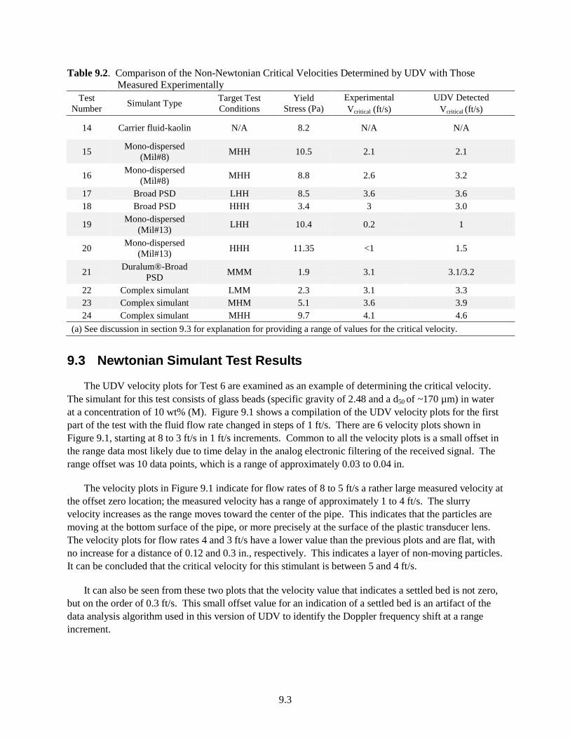
9.3

Table 9.2. Comparison of the Non-Newtonian Critical Velocities Determined by UDV with Those Measured Experimentally


Conditions Yield

Stress (Pa) Experimental Vcritical (ft/s)

UDV Detected Vcritical (ft/s)

14 Carrier fluid-kaolin N/A 8.2 N/A N/A

15 Mono-dispersed (Mil#8) MHH 10.5 2.1 2.1

16 Mono-dispersed (Mil#8) MHH 8.8 2.6 3.2

17 Broad PSD LHH 8.5 3.6 3.6 18 Broad PSD HHH 3.4 3 3.0

19 Mono-dispersed (Mil#13) LHH 10.4 0.2 1

20 Mono-dispersed (Mil#13) HHH 11.35 <1 1.5

21 Duralum®-Broad PSD MMM 1.9 3.1 3.1/3.2

22 Complex simulant LMM 2.3 3.1 3.3 23 Complex simulant MHM 5.1 3.6 3.9 24 Complex simulant MHH 9.7 4.1 4.6

(a) See discussion in section 9.3 for explanation for providing a range of values for the critical velocity.

9.3 Newtonian Simulant Test Results

The UDV velocity plots for Test 6 are examined as an example of determining the critical velocity. The simulant for this test consists of glass beads (specific gravity of 2.48 and a d50 of ~170 µm) in water at a concentration of 10 wt% (M). Figure 9.1 shows a compilation of the UDV velocity plots for the first part of the test with the fluid flow rate changed in steps of 1 ft/s. There are 6 velocity plots shown in Figure 9.1, starting at 8 to 3 ft/s in 1 ft/s increments. Common to all the velocity plots is a small offset in the range data most likely due to time delay in the analog electronic filtering of the received signal. The range offset was 10 data points, which is a range of approximately 0.03 to 0.04 in.

The velocity plots in Figure 9.1 indicate for flow rates of 8 to 5 ft/s a rather large measured velocity at the offset zero location; the measured velocity has a range of approximately 1 to 4 ft/s. The slurry velocity increases as the range moves toward the center of the pipe. This indicates that the particles are moving at the bottom surface of the pipe, or more precisely at the surface of the plastic transducer lens. The velocity plots for flow rates 4 and 3 ft/s have a lower value than the previous plots and are flat, with no increase for a distance of 0.12 and 0.3 in., respectively. This indicates a layer of non-moving particles. It can be concluded that the critical velocity for this stimulant is between 5 and 4 ft/s.

It can also be seen from these two plots that the velocity value that indicates a settled bed is not zero, but on the order of 0.3 ft/s. This small offset value for an indication of a settled bed is an artifact of the data analysis algorithm used in this version of UDV to identify the Doppler frequency shift at a range increment.

9.4

Figure 9.2 show the UDV data plots for the second part of Test 6 where the flow rate was decreased in 0.1 ft/s steps to zoom into the velocity range where the flow transitions between a condition where the particles are still moving to a condition where a settled bed is formed. It can be seen from the plots in this figure that slurry flow rates of 4.4 and 4.3 ft/s indicate a velocity of about 0.49 to 0.56 ft/s at the offset zero location and the velocity increases as we move away toward the center of the pipe. Similarly, the velocity plot for 4.2 ft/s is lower and varies between 0.3 and 0.49 ft/s for fractions of an inch before increasing in velocity. The data plots for 4.1 to 3.9 ft/s indicate a thin settled bed that increases in thickness with decreasing flow. Since 4.1 ft/s velocity data plot is the highest flow rate to have values that indicate a stable settled bed has formed, it is identified as the Vcritical condition.

Figure 9.1. Test 6 Summary Velocity Plot for 1 ft/s Flow Rate Increments.

9.5

Figure 9.2. Test 6 Summary Velocity Plot for 0.1 ft/s Flow Rate Increments.

The UDV data for Test 12 is an example where the UDV determination of critical velocity was bracketed by a range rather than a single value as indicated by the experimental data. To understand this better, the velocity plots for Test 12 are discussed. The simulant for this test consisted of a mixture of Potters glass beads (specific gravity of 2.50 g/mL and a broad PSD with d50 of 94 µm) at a concentration of 20 wt% (H) of glycerin/water (specific gravity of 1.15 and viscosity of 11.7 mPa.s).

Figure 9.3 shows a compilation of the UDV velocity plots for the first part of the test, where the fluid flow rate was changed in steps of 1 ft/s. Similarly, Figure 9.4 shows the second part of Test 12, where the flow rate was decreased in 0.1 ft/s steps to study the region where the near-critical and critical flow behavior occurs.

It can be seen from the data in Figure 9.3 that between 3 and 2 ft/s there is a clear transition from where the entire slurry is moving to a condition where a settled bed as indicated by a region where the velocity data is not changing. The data in Figure 9.4 shows a thickening layer of slow moving particles as the flow rate is lowered from 2.8 to 2.5 ft/s. The velocity plots in Figure 9.4 do not show the characteristic flat stable velocity that was seen at 2 ft/s (cf. Figure 9.3) or with other Newtonian simulants (for example, see Figure 9.1 and Figure 9.2). This, coupled with the facts that (1) a clear bed was observed at 2 ft/s, and (2) no data was collected between 2.5 and 2 ft/s, led to the determination that the critical velocity was between 2.5 and 2 ft/s. Additional data points needed to be collected between 2.5 and 2 ft/s to allow for further refinement of the critical velocity for this test. However, if one were to

9.6

expand the definition of critical velocity to a very slowly sliding or pulsating (stop and go) bed that increases in thickness with time (i.e., include Regimes II and III as discussed in section 6), it can be seen from the data in Figure 9.4 that the UDV velocity plots at slurry velocities between 2.8 ft/s to 2.5 ft/s exhibit such behavior. It can therefore be argued that UDV is not only sensitive to detect critical velocities but can give the operators a clear indication of the onset of particle settling.

Note that the UDV velocity profile data for Test 13 also resulted in range for the critical velocity determination for the same reasons as Test 12.


9.7


9.4 Non-Newtonian Simulant Test Results

The UDV system operating at 1 MHz did not detect scattered ultrasound from the kaolin mixture exclusively. Therefore, the kaolin mixture should act as a carrier similar to the water or glycerin/water fluid used in the Newtonian tests; only the simulant particles added to the carrier fluid should cause a Doppler frequency shift. This is explained by the fundamental requirements for ultrasonic scattering, similar to those discussed for the PulseEcho system in section 7.0; however, the UDV system can utilize weak scattering as well as strong scattering to perform its measurements. The kaolin mixture did significantly attenuate the UDV ultrasound tone burst signal, requiring UDV to be operated at a higher gain setting to get an adequate receive signal scattered from the particles. This leads to increased noise in the receive signal compared to the Newtonian tests.

The UDV data from Test 15 will be used as an example of how to interpret the velocity data to determine Vcritical for the non-Newtonian tests. The simulant for this test consisted of Potters Ballotini glass beads (specific gravity of 2.50 g/mL and a d50 of ~94 µm) at a concentration of 10 wt% (M) dispersed in a carrier fluid consisting of ~25 wt% kaolin in water. Figure 9.5 presents a compilation of the UDV velocity plots for Test 15 for the first part of the test when the fluid flow rate was changed in 1 ft/s steps. There are seven velocity plots shown in Figure 9.5, spanning 8 to 2 ft/s. Similarly, Figure 9.6 shows the second part of Test 15, where the flow rate was decreased in steps of 0.1 ft/s to zoom in on the

9.8

actual velocity where the critical behavior is more closely investigated. From the data in Figure 9.5, it can be concluded that the critical velocity lies between 3 and 2 ft/s.


9.9


Looking at the zoomed-in plots in Figure 9.6, it can be seen that at slurry velocities ranging from 2.4 to 2.2 ft/s indicate a slow moving layer on the bottom of the pipe with a velocity less than 0.16 ft/s (5 cm/s). The velocity plot for 2.1 ft/s indicates a stable layer on the bottom of the pipe. Since the 2.1 ft/s velocity data is the highest flow velocity to have values that indicate a settled layer has formed, it is identified as the Vcritical condition. Again, using the same arguments presented in section 9.2.1 when discussing the Test 12 data, it can be argued that at velocities of 2.4 to 2.2 ft/s the flow characteristics represent a sliding bed with increasing bed thickness and decreasing slurry velocity.

Test 18 is another example that illustrates the potential of the UDV technique. The simulant for this test consists of Potters spheres with a broad particle distribution (specific gravity of 2.50 and a d50 of ~292 µm) at a concentration of 20 wt% (H) dispersed in a carrier fluid consisting of ~25 wt% kaolin in water. Figure 9.7 shows a compilation of the UDV velocity plots for the first part of the Test 18 where the fluid flow rate was decreased in steps of 1 ft/s. Similarly, Figure 9.8 shows the second part of Test 18 where the flow rate was decreased in steps of 0.1 ft/s steps.

9.10


From the data in Figure 9.7, it can be concluded that Vcritical for Test 18 occurs between 3 and 2 ft/s. From the zoomed-in data in Figure 9.8, it can be seen that a clear flat region in the UDV profile occurs at a velocity of 2.9 ft/s and is therefore identified as the critical velocity. Once again, using the same arguments presented in section 9.2.1 when discussing the Test 12 data, the data in Figure 9.8 suggests that at a velocity of 3.2 ft/s a sliding bed is present with increasing bed thickness as slurry velocity is decreased.

9.11


10.1

10.0 Future Development and Field Deployment Considerations

The following are some of the general issues that need to be addressed before any of the three PNNL-developed instruments evaluated in the present study can be deployed in the highly radioactive environments that will be encountered during waste transfer operations:

1. Expanding sensitivity of instruments to detect < 30 micron particulates of very high densities (i.e., on the order of the density of PuO)

a. Build up PuO over the length of the transfer section is not a desirable outcome during the slurry transfer operations since it could lead to undesirable concentrations of PuO in the transfer vessel or receipt vessel during flushing operations.

b. This will require the evaluation of multi-transducer configurations; the primary configuration looking at large (>50 µm) particles while the secondary focusing on the settling and agglomeration of small ~30 µm particulates very close to the wall region.

2. Establishing long term performance and reliability of the instruments to detect critical velocities and settled bed formation. One example of an operating guideline is determining the degree of pipe fouling by checking instrumentation pipe-wall reference values during pipeline flushing with water. Undetected pipe fouling and neglecting subsequent reference updates can result in incorrect measurements or false indications of sedimentation.

3. Evaluating the instruments using simulants that are engineered to more closely mimic the actual properties of expected WTP high-level waste feed batches.

a. This recommendation is specifically geared toward testing sensor performance using one or more simulants that mimic real waste properties to further strengthen the applicability of these sensors to determine critical velocities during the real waste transfer applications.

4. Determining the lower solids concentration limit for the UDV and PulseEcho systems by performing testing with very dilute slurries

The UDV and PulseEcho systems rely on ultrasonic scattering from slurry particles to perform their

measurements. The ability to perform scattering measurements will not be affected by environmental temperature fluctuations unless there is a bulk physical phase change (i.e., liquid to solid) of the process stream. The Attenuation system relies on measuring the combined effect of absorption and scattering (attenuation) of an ultrasonic pulse after it has propagated across the instrumentation spool piece in the certification flow loop. Attenuation generally decreases with increasing temperature, and can also be affected by a bulk physical change of the process stream.

In addition to the above, there are specific developments that are required for each instrument and are

discussed below.

10.2

10.1 PulseEcho Ultrasound Development Requirements

The ultrasonic PulseEcho system is a laboratory prototype unit that has been used on pilot-scale engineering support projects at PNNL and has been operated primarily by those skilled in the operation of such ultrasonic devices and measurement equipment. To prepare the PulseEcho system for field deployment, the following improvements and modifications are required:

1. One of the main concerns, particularly with the “as tested” PulseEcho system is its ability to detect critical velocities in slurries with very low solids concentrations, such as those possibly encountered during the transfers of very dilute low-activity waste. Of particular concern here is whether there is a lower limit in the solids concentration below which the PulseEcho system would be impractical. An obvious solution to the issue is to increase the inventory of scatterers within the insonified fluid volume by increasing the size of the transducer. In other words, the larger the transducer, the lower the solids concentration at which the PulseEcho system would be applicable. However large, particularly flat transducers introduce additional design challenges since mounting such transducers to the bottom of the pipe section will require significant reduction or modifications of the pipe wall to ensure that the transducer is mounted on flat section of pipe. Other sensor geometries are available that could prove more optimum for pipeline fitting and inspection volume, such as rectangular sensors that run axially along the bottom of the pipe thereby reducing the negative pipe curvature effects exhibited on larger round sensors. Therefore a trade-off among transducer size, mounting options, and improvement in the sensitivity of the PulseEcho system needs to be determined to find the optimal transducer size and configuration and also establish the lower limit for the PulseEcho system applicability. This will require additional flow loop testing.

2. Evaluate options (such as curved transducers) to utilize the full schedule 40 pipe wall thickness for installing the non-invasive transducers as opposed to locally reducing wall thickness. This will require additional flow loop testing.

3. The PulseEcho data acquisition hardware currently experiences artificial digitizer jitter in the time domain of the ultrasonic signals. This system artifact can be addressed by reconfiguring the data acquisition hardware to receive a trigger from a function generator in place of the ultrasonic pulser trigger. Following reconfiguration, the PulseEcho algorithm should be validated again. This can be resolved without additional flow loop testing.

4. The ultrasonic signals received by the PulseEcho digitizer card appear saturated in the data display due to a 1 volt peak-to-peak digitizer setting that is below the maximum amplitude of the received ultrasonic signals. This issue can be addressed by adjusting the peak-to-peak voltage on digitizer to eliminate signal saturation.

5. Replace the currently utilized analog pulser with a digital pulser in order to provide a more stable pulse voltage to the PulseEcho transducer for the purpose of eliminating signal drift.

6. Simplify and streamline data logging/compilation and file saving. The PulseEcho program currently has to be stopped and restarted to generate new data files.

10.3

7. Address long-term transducer bonding and coupling to the pipe. Epoxy has been used at PNNL to couple and bond PulseEcho transducers to a vessel or pipe, which is likely acceptable for short-term testing only.

10.2 Ultrasonic Attenuation Development Requirements

The ultrasonic attenuation system in its present state is not entirely suitable for use for the Hanford tank waste transfer application. In order to facilitate the application of the technology, advanced software modifications will be required to translate the Vs/Vw and the NSTD information into reliable signals to detect critical velocities. Despite the simplicity of the attenuation sensor and its non-invasive nature, this sensor requires significant development before field deployment should be considered.

10.3 Ultrasonic Doppler Velocimetry Development Requirements

The following items need to be addressed regarding the UDV system prior to field deploying the technology:

1. The operating and radiation environment of the actual certification loop test system will impact the UDV system. The interface material, either Rexolite® or PEEK, will be exposed to wear and physical damage from the particles in the slurry. An estimate of the roughness or pitting that can occur needs to be determined so that signal changes, inducing variations in velocity calculations, can be established to understand the effect due to the interface surface not being smooth.

2. Refine the lens design to optimize the transducer/sleeve configuration and minimize internal reflections of the ultrasound signal.

3. Although most comments received concerning using Rexolite® and PEEK in a radiation environment were positive, radiation exposure may change the material properties that would affect the ultrasound signals passing through it. Characterization of speed of sound and attenuation parameters before and after exposure to radiation needs to be performed.

4. Ultrasound transducer validation needs to be done in a typical radiation environment expected on the waste certification loop. The main concern is signal degradation and increased signal noise caused by radiation.

5. Upgrading the data acquisition system currently being used in the UDV system since the configuration that was used in the present testing was from the first generation of the UDV system and is quite dated by today’s standards.

6. Evaluation of long term wear and radiation degradation of the interface material (i.e., lens) at the interface to maintain primary containment of the waste slurry.

10.4 Field Deployment Considerations

This section specifically deals with issues that need to be addressed to make the technologies suitable for use in the waste certification loop at the tank farms.

10.4

1. Radiation hardening and shielding of ultrasonic elements and associated components located closest to the waste certification loop

2. Developing integral design of instrument spool pieces to facilitate easy, problem-free, integration into the waste certification loop

3. Remote operation of the transducers. This will require:

a. development of requirements for establishing communications between the local and remotely located instruments to facilitate transducer pulsing and signal capture from the transducers, and

b. development and testing of remotely operated systems.

11.1

11.0 Conclusions and Recommendations

This report presents the evaluation of three PNNL-developed sensors for the detection of critical velocity and settled bed formation during the transfer of highly radioactive waste slurries from the Hanford DSTs to the WTP. The ultrasonic sensors evaluated were (1) PulseEcho, (2) Ultrasonic Attenuation, and (3) Ultrasonic Doppler Velocimeter. The assessment of the ultrasonic sensor performance was conducted using a wide variety of simulants that have particle-size, density (to a limited extent), and non-Newtonian rheological property values similar to those expected during the Hanford tank retrieval operations.

A total of 25 tests (including 1 repeat test) were performed to assess the performance of the three ultrasonic instruments. Table 11.1 presents an overview of the critical velocities for all the Newtonian simulant tests as measured by the three ultrasonic instruments along with the experimentally measured critical velocities. The data for the non-Newtonian simulants is shown in Table 11.2. Note that on several tests a range was reported for the visual observation for the critical velocity (i.e., stationary bed formation). During these tests, a stationary bed did not form at the same time in the upstream and downstream visualization sections. Thus, a range was reported that captures the velocities of when the bed formed in the upstream and downstream sections. Also included in this table are the velocity information for focused axial motion (Regime II as discussed in section 6) and a pulsating bed (Regime III as discussed in section 6); which are typically indicators of the onset of critical velocity.

In Table 11.1 and Table 11.2, a match between the experimental range for Regime II, Regime III, and Vcrit and the ultrasonic sensor measurement is considered excellent and is shown by shading the cells in green. Similarly, if the ultrasonic sensor measurement falls within ± 0.3 ft/s of this range, the measurement was still considered good and indicated by shading the cells in amber. Finally, if an ultrasonic measurement falls outside this range, the measurement was considered poor and indicated by shading the cells in red. Such a green/amber/red shading of the cells provides a quick assessment of the sensor performance.

It can be seen from the data in Table 11.1 and Table 11.2, both the PulseEcho and the UDV systems do an excellent job in matching with the experimentally observed critical velocities. It can also be seen from the data in these tables, for situations designated amber or red in the PulseEcho or UDV data, the errors are minor or in flow ranges that are far below those that would be of concern during slurry transfer operations (i.e., << 1 ft/s).

Based on the performance observed, both PulseEcho and UDV are considered excellent candidates for use in the waste certification loop. PulseEcho and UDV systems complement one another well, one displaying strengths where the other displays weaknesses and vice versa based on slurry solids concentration. Therefore, it is highly recommended that both these instruments be collectively considered for further development into an integrated field deployable unit to offer the largest possible span of detection accuracy. Besides facilitating detection resolution in the event of inconclusive measurements from one sensor based on solids concentration, the application of both instruments provides detection confirmation/redundancy. Therefore, both of these sensing technologies are recommended for the next phase of prototypic system testing that will identify and resolve field deployment requirement.

11.2

If further development of more than one sensor type is not practical, then PulseEcho would be the preferred instrument for field deployment. This is because the PulseEcho system has a distinct advantage over the UDV system in terms of the simplicity in its mounting requirements; the PulseEcho transducer can be mounted on the outside of pipe whereas the UDV system requires breaching the pipe to mount the sensor assembly that includes a Rexolite® or PEEK lens. In following this path, however, it should be remembered that PulseEcho system “as tested” is prone to false indications of critical velocity with slurries containing low solids concentrations such as those possibly encountered during the transfers of very dilute low-activity waste. On the other hand, the UDV system works best at very low solids concentrations, where just a few scatters are sufficient to produce a good signal. Although there are ways to improve the performance of the PulseEcho system at low concentrations by increasing the inventory of scatterers within the insonified fluid volume by increasing the size of the transducer, the tradeoffs among transducer size, mounting options, and improvement in the sensitivity of the PulseEcho system are yet unknown and need to be established.

Finally, the configuration of the sensors tested was not optimized for field deployment. The specific issues that need to be addressed for each sensor along with the general issues associated with adaptation of any sensor to a radiological application are discussed in section 10, Future Development and Field Deployment Considerations. For example, additional testing is needed to enable detection of the settling of heavy (specific gravity > 8) particles in the 10 to 30 µm size and optimizing sensor configuration for critical velocity detection at low solids concentrations. Resolution of hardware issues, such as modernization of the UDV system and upgrading the PulseEcho pulser to digital, would also be required. Additional testing with smaller particles and very dilute solids concentrations is required in order to further test the limitations of the recommended instruments against the ranges of representative Hanford tank waste. In addition, radiation hardening of the ultrasonic transducers and cables would be required for field deployment. PNNL has worked with vendors to specify radiation hardened transducers and cables for prior research projects. Furthermore, instrument configuration and sizing must be optimized to ensure adequate implementation and operation in the field. As such, it is recommended that these optimized instruments be integrated into modular spool pieces that can be easily pre-checked in the cold certification test loop before implementation in the field.

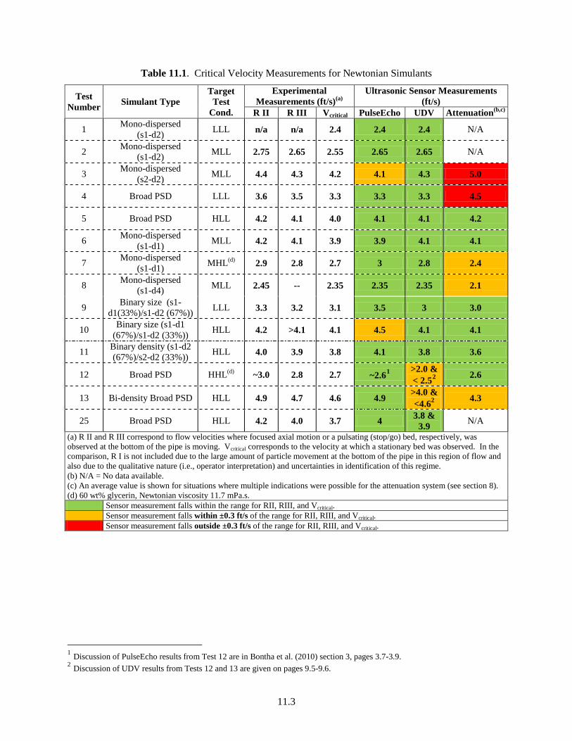
11.3

Table 11.1. Critical Velocity Measurements for Newtonian Simulants

Test Number Simulant Type

Target Test

Cond.

Experimental Measurements (ft/s)(a)

Ultrasonic Sensor Measurements (ft/s)

R II R III Vcritical PulseEcho UDV Attenuation(b,c)

1 Mono-dispersed (s1-d2) LLL n/a n/a 2.4 2.4 2.4 N/A

2 Mono-dispersed (s1-d2) MLL 2.75 2.65 2.55 2.65 2.65 N/A

3 Mono-dispersed (s2-d2) MLL 4.4 4.3 4.2 4.1 4.3 5.0

4 Broad PSD LLL 3.6 3.5 3.3 3.3 3.3 4.5

5 Broad PSD HLL 4.2 4.1 4.0 4.1 4.1 4.2

6 Mono-dispersed (s1-d1) MLL 4.2 4.1 3.9 3.9 4.1 4.1

7 Mono-dispersed (s1-d1) MHL(d) 2.9 2.8 2.7 3 2.8 2.4

8 Mono-dispersed (s1-d4) MLL 2.45 -- 2.35 2.35 2.35 2.1

9 Binary size (s1-d1(33%)/s1-d2 (67%)) LLL 3.3 3.2 3.1 3.5 3 3.0

10 Binary size (s1-d1 (67%)/s1-d2 (33%)) HLL 4.2 >4.1 4.1 4.5 4.1 4.1

11 Binary density (s1-d2 (67%)/s2-d2 (33%)) HLL 4.0 3.9 3.8 4.1 3.8 3.6

12 Broad PSD HHL(d) ~3.0 2.8 2.7 ~2.61 >2.0 & < 2.5 2 2.6

13 Bi-density Broad PSD HLL 4.9 4.7 4.6 4.9 >4.0 & <4.62 4.3

25 Broad PSD HLL 4.2 4.0 3.7 4 3.8 & 3.9 N/A

(a) R II and R III correspond to flow velocities where focused axial motion or a pulsating (stop/go) bed, respectively, was observed at the bottom of the pipe is moving. Vcritical corresponds to the velocity at which a stationary bed was observed. In the comparison, R I is not included due to the large amount of particle movement at the bottom of the pipe in this region of flow and also due to the qualitative nature (i.e., operator interpretation) and uncertainties in identification of this regime. (b) N/A = No data available. (c) An average value is shown for situations where multiple indications were possible for the attenuation system (see section 8). (d) 60 wt% glycerin, Newtonian viscosity 11.7 mPa.s. Sensor measurement falls within the range for RII, RIII, and Vcritical. Sensor measurement falls within ±0.3 ft/s of the range for RII, RIII, and Vcritical. Sensor measurement falls outside ±0.3 ft/s of the range for RII, RIII, and Vcritical.

1 Discussion of PulseEcho results from Test 12 are in Bontha et al. (2010) section 3, pages 3.7-3.9. 2 Discussion of UDV results from Tests 12 and 13 are given on pages 9.5-9.6.

11.4

Table 11.2. Critical Velocity Measurements for Non-Newtonian Simulants.

Test # Simulant Type Target

Test Cond.

Yield Stress (Pa)

Experimental Measurement Velocities

(ft/s)(a,b)

Ultrasonic Sensor Measurements (ft/s)

R II R III Vcritical PulseEcho UDV Attenuation(c)

14 Carrier fluid-kaolin N/A 8.2 -- -- -- -- -- --

15 Mono-dispersed (Mil#8) MHH 10.5 -- -- 2.1-2.3 2.1 2.1 N/A

16 Mono-dispersed (Mil#8) MHH 8.8 4.0 3.2 2.6-3.0 3.2 3.2 N/A

17 Broad PSD LHH 8.5 4.2 -- 3.6 4.1 3.6 4.2

18 Broad PSD HHH 3.4 3.5 3.1 3.0 3.3 3 2.8

19 Mono-dispersed (Mil#13) LHH 10.4 -- 0.3 0.2 0.5 1 0.4

20 Mono-dispersed (Mil#13) HHH 11.35 -- 1.4 <1.0 1.5 1.5 1.2

21 Duralum-Broad PSD MMM 1.9 3.5 3.4 3.1-3.3 3.2 3.1 &

3.2 2.8

22 Complex simulant LMM 2.3 3.5 3.4 3.1-3.3 3.3 3.3 3.3

23 Complex simulant MHM 5.1 4.3 4.2 3.6-3.8 3.9 3.9 4.4

24 Complex simulant MHH 9.7 5.0 4.2 4.1-4.7 4.3 4.6 4.4

(a) R II and R III correspond to flow velocities where focused axial motion or a pulsating (stop/go) bed, respectively, was observed at the bottom of the pipe is moving. Vcritical corresponds to the velocity at which a stationary bed was observed. In the comparison, R I is not included due to the large amount of particle movement at the bottom of the pipe in this region of flow and also due to the qualitative nature (i.e., operator interpretation) and uncertainties in identification of this regime. (b) N/A = No data available. (c) An average value is shown for situations where multiple indications were possible for the attenuation system (see section 8). Sensor measurement falls within the range for R II, RIII, and Vcritical. Sensor measurement falls within ± 0.3 ft/s of the range for R II, RIII, and Vcritical. Sensor measurement falls outside ± 0.3 ft/s of the range for R II, RIII, and Vcritical.

12.1

12.0 References

Bamberger J, M Greenwood, G Morgen, P Meyer, E Baer, M Minette, P Scott. 2009. “Insitu Measurement Techniques for Characterizing Pulse Jet Mixing of Slurries.” FEDSM2009-78585. In Proceedings of the ASME 2009 Fluids Engineering Division Summer Meeting. August 2-6, 2009. Vail, CO.

Bamberger JA, and MS Greenwood. 2001. Development of a Density Sensor for In-Line Real-Time Process Control and Monitoring of Slurries during Radioactive Waste Retrieval and Transport Operations at DOE Sites. PNNL-13719, Pacific Northwest National Laboratory, Richland, WA. Bamberger JA, and MS Greenwood. 2004. “Measuring Fluid and Slurry Density and Solids Concentration Non-Invasively.” Ultrasonics 42:563-567.

Bond LJ, M Meenaksh, and HO Matthiesen. 1998. “Ultrasonic methods for the on-line real-time characterization of state of mixing.” In Proceeding 16th ICA and 135th meeting Acoustical Society of America, June 20-26, 1998. Ed. P.K. Kuhl and L.A. Crum. pp 1161-1162. Seattle, WA.

Bontha JR, HE Adkins, KM Denslow, JJ Jenks, CA Burns , PP Schonewill, GP Morgen, MS Greenwood, J Blanchard, TJ Peters, PJ MacFarlan, EB Baer, WA Wilcox. 2010. Supplementary Information for Test Loop Demonstration and Evaluation of Slurry Transfer Line Critical Velocity Measurement Instruments. PNNL-19560, Pacific Northwest National Laboratory, Richland, WA.

Greenwood MS, and JA Bamberger. 2002. “Measurement of Viscosity and Shear Wave Velocity of a Liquid or Slurry for On-line Process Control.” Ultrasonics 39:623-630.

Greenwood MS, and JA Bamberger. 2004. “Self-calibrating Sensor for Measuring Density through Stainless Steel Pipeline Wall.” Journal of Fluids Engineering-Transactions of the ASME 126:189-192.

Greenwood MS, JD Adamson, and JA Bamberger. 2006. “Long-path measurements of ultrasonic attenuation and velocity for very dilute slurries and liquids and detection of contaminates.” Ultrasonics 44:e461-e466.

Greenwood MS. 2004. “Self Calibrating System and Technique for Ultrasonic Determination of Fluid Properties.” U.S. Patent 6,763,698.

Hall MN. 2008. ICD-19 – Interface Control Document for Waste Feed. 24590-WTP-RPT-PE-07-001. Bechtel National, Inc. Richland, WA.

Hauptmann P, N Hoppe, and A Puttmer. 2002. Meas. Sci. Technol. 13 (2002) R73.

Hauptmann P, R Lucklum, and A Puttmer, and B Henning. 1998. Sensor. Actuat. A 67 (1998) 32.

Lynnworth LC, G Jossinet, and E Cherifi. 1996. IEEE Ultrason. Symp. (1996) 407.

McClements DJ. 1997. Critical Rev. Food Sci. Nutrition 37 (1997) 1.

Meyer PA, HE Adkins, KM Denslow, JA Bamberger, BE Wells, MS Greenwood, PA Scott, J Blanchard, GP Morgen. 2009a. Hanford Tank Farms Waste Certification Flow Loop Test Strategy. PNNL-18688, Pacific Northwest National Laboratory, Richland, WA.

12.2

Meyer PA, JA Bamberger, CW Enderlin, JA Fort, BE Wells, SK Sundaram, PA Scott, MJ Minette, GL Smith, CA Burns, MS Greenwood, GP Morgen, EBK Baer, SF Snyder, M White, GF Piepel, BG Amidan, A Heredia-Langner. 2009b. Pulse Jet Mixing Tests With Noncohesive Solids, PNNL-18098 (WTP-RPT-182 Rev. 0), Pacific Northwest National Laboratory, Richland, WA.

Morgen GP, RA Pappas, DM Pfund, WC Weimer, DM Sheen, and BJ Burghard. 2005. “Ultrasonic System and Technique for Fluid Characterization.” U.S. Patent 6,871,148 B2

Panetta PD, BJ Tucker, KM Denslow, LW Burgess, AM Brodsky, and SL Randall. 2005. Physical Characterization of Solid-Liquid Slurries at High Weight Fractions Using Optical and Ultrasonic Methods. Department of Energy-Environmental Molecular Sciences Program, Grant 81964 Annual Report.

Pappas RA, LJ Bond, MS Greenwood, and CJ Hostick. 2007. On-line physical property measurements for nuclear fuel recycling, GLOBAL 2007, Advanced Nuclear Fuel Cycles and Systems, Boise, ID, September 9-13, 2007, Am. Nuclear Soc. pp 1808-1816.

Pfund DM, MS Greenwood, JA Bamberger, RA Pappas. 2007. Ultrasonics 44 (2006) e477 - e482, Inline Ultrasonic Rheometry by Pulsed Doppler.

Poloski AP, HE Adkins, J Abrefah, AM Casella, R Hohimer, F Nigl, MJ Minette, JJ Toth, JM Tingey, and SM Yokuda. 2009a. Deposition Velocities of Non-Newtonian Slurries in Pipelines. PNNL-17639, WTP-RPT-175 Rev. 0. Pacific Northwest National Laboratory, Richland, WA.

Poloski AP, ML Bonebrake, AM Casella, MD Johnson, JJ Toth, HE Adkins, Jr, J Chun, KM Denslow, M Luna, and JM Tingey. 2009b. Deposition Velocities of Non-Newtonian Slurries in Pipelines: Complex Simulant Testing . PNNL-18316, WTP-RPT-189 Rev. 0. Pacific Northwest National Laboratory, Richland, WA.

Port Plastics. 2009. Rexolite® Crosslinked Polystyrene Product Properties Sheet. http://www.portplastics.com/plastics/commodities/RexoliteC-L.html. Accessed October 20, 2009.

Povey M., Semin. 1999. Food Analysis 4 (1999) 95.

Rae, PJ, EN Brown, and EB Orler. 2007. The mechanical properties of poly(ether-ether-ketone) (PEEK) with emphasis on the large compressive strain response, Polymer 48 pp. 598-615.

Shekarriz A, and DM Sheen. 1998. “Slurry Pipe Flow Measurements Using Tomographic Ultrasonic Velocimetry and Densitometry.” FEDSM98-5076. In Proceedings of FEDSM ’98 (1998 ASME Fluids Engineering Division Summer Meeting, June 1998).

Shekarriz A, and DM Sheen. 2000. “Method and Apparatus for Ultrasonic Doppler Velocimetry using Speed of Sound and Reflection Mode Pulsed Wideband Doppler.” U.S. Patent 6,067,861.

Stolojanu V, and A Prakash. 2001. Chemical Engineering Journal 84, pp. 215-222.

Torres, TD. 2003. Evaluation of Hose-in-Hose Transfer Line Service Life. RPP-6711 Rev. 2, Appendix C-7. COGEMA Engineering Corporation, Richland, WA.

http://www.portplastics.com/plastics/commodities/RexoliteC-L.html�

12.3

Ulrick, RJ. 1975. Principles of Underwater Sound, McGraw-Hill Book Company.

Urick RJ. 1947. J. Phys. D: Appl. Phys. 18 (1947) 983.

Workman J Jr., DJ Veltkamp, S Doherty, BB Anderson, KE Creasy, M Koch, JF Tatera, AL Robinson, L Bond, LW Burgess, GN Bokerman, AH Ullman, GP Darsey, F Mozaynei, JA Bamberger, MS Greenwood. 1999. Analytical Chemistry 71 (1999) 121R-180R.

Workman J Jr., KE Creasy, S Doherty, L Bone, M Koch, A Ullman, DJ. 2001. Veltkamp, Analytical Chemistry 73 (2001) 2705.

Yokuda ST, AP Poloski, HE Adkins, AM Casella, RE Hohimer, NK Karri, M Luna, MJ Minette, and JM Tingey. 2009. A Qualitative Investigation of Deposition Velocities of a Non-Newtonian Slurry in Complex Pipeline Geometries. PNNL-17973, WTP-RPT-178, Rev. 0, Pacific Northwest National Laboratory, Richland, WA.

PNNL-#####

Distribution

No. of No. of Copies Copies

Distr.1

20 Pacific Northwest National Laboratory JR Bontha (10) P7-25 CA Burns P7-25 HE Adkins K7-15

J Blanchard K7-15 KA Denslow K5-26 MS Greenwood K5-26 JJ Jenks K7-15 GP Morgen K5-17 P Schonewill P7-25 BE Wells K7-15 PA Scott K7-15

6 Washington River Protection Solutions M Thien (5) B1-55 T Wooley (1) B1-55 2 Office of River Protection (DOE) JS Shuen (2) H6-60

slurry transfer line critical velocity measurement instruments

Documents