Slightly beyond Turing-Computability for studying

Genetic Programming

Olivier Teytaud

To cite this version:

Olivier Teytaud. Slightly beyond Turing-Computability for studying Genetic Programming.MCU’07, 2007, Orleans, France. 2007. <inria-00173241>

HAL Id: inria-00173241

https://hal.inria.fr/inria-00173241

Submitted on 19 Sep 2007

HAL is a multi-disciplinary open accessarchive for the deposit and dissemination of sci-entific research documents, whether they are pub-lished or not. The documents may come fromteaching and research institutions in France orabroad, or from public or private research centers.

L’archive ouverte pluridisciplinaire HAL, estdestinee au depot et a la diffusion de documentsscientifiques de niveau recherche, publies ou non,emanant des etablissements d’enseignement et derecherche francais ou etrangers, des laboratoirespublics ou prives.

brought to you by COREView metadata, citation and similar papers at core.ac.uk

provided by HAL-Polytechnique

Slightly beyond Turing’s computability for

studying genetic programming

Olivier Teytaud

TAO, INRIA Futurs, LRI, UMR 8623 (CNRS - Univ. Paris-Sud),olivier.teytaud@inria.fr

Abstract. Inspired by genetic programming (GP), we study iterativealgorithms for non-computable tasks and compare them to naive models.This framework justifies many practical standard tricks from GP and alsoprovides complexity lower-bounds which justify the computational costof GP thanks to the use of Kolmogorov’s complexity in bounded time.

1 Introduction

Limits of Turing-computability are well-known [28, 20]; many things of inter-est are not computable. However, in practice, many people work on designingprograms for solving non-computable tasks, such as finding the shortest pro-gram performing a given task, or the fastest program performing a given task:this is the area of genetic programming (GP) [9, 13, 15]. GP in particular pro-vides many human-competitive results (http://www.genetic-programming.com/humancompetitive.html), and contains 5440 articles by more than 880authors according to the GP-bibliography [5]. GP is the research of a programrealizing a given target-task roughly as follows:

1. generate (at random) an initial population of algorithms ;2. select the ones that, after simulation, are “empirically” (details in the sequel)

the most relevant for the target-task (this is dependent of a distance betweenthe results of the simulation and the expected results, which is called thefitness) ;

3. create new programs by randomly combining and randomly mutating theones that remain in the population ;

4. go back to step 2.

Theoretically, the infinite-computation models [6] are a possible model forstudying programs beyond the framework of Turing Machines (TM). However,these models are far from being natural: they are intuitively justified by e.g.time steps with duration divided by 2 at each tick of the clock. We here work onanother model, close to real-world practice like GP: iterative programs. Theseprograms iteratively propose solutions, and what is studied is the convergence ofthe iterates to a solution in ≡f with good properties (speed, space-consumption,size), and not the fact that after a finite time the algorithm stops and proposesa solution. The model, termed iterative model, is presented in algorithm 1. We

point out that we can’t directly compare the expressive power of our model andthe expressive power of usual models of computation; we here work in the frame-work of symbolic regression. Classically, programs work with a program as input,and output something (possibly a program). Here, the input can be a program,but it can also be made of black-box examples provided by an oracle. Therefore,we study algorithms with: (i) inputs, provided by an oracle (precisely, the or-acle provides examples (xi, f(xi))); (ii) possibly, an auxiliary input, which is aprogram computing f ; (iii) outputs, which are programs supposed to convergeto the function f underlying the oracle and satisfying some constraints (e.g.asymptotically optimal size or asymptotically optimal speed). This is symbolicregression. We can encode decision problems in this framework (e.g., deciding if∀n, f(n) = 1 by using xi independent and ∀n ∈ N, P (xi = n) > 0); but we cannot encode the problems as above as decision problems or other classical familiesof complexity classes. However, the links with various Turing degrees might bestudied more extensively than in this paper.

Algorithm 1 GP - Iterative-algorithmsSet p = 1.while true do

Read an input Ip = (xp, yp) with yp = f(xp) on an oracle-tape.Perform standard computations of a TM (allowing reading and writing on aninternal tape).Output some Op.p← p + 1

end while

This model is the direct translation of genetic programming in a Turing-likeframework. A different approach consists in using also f as input. Of course,in that case, the important point is that Op is “better” than f (faster, morefrugal in terms of space-consumption, or smaller). We will see that at least inthe general framework of f Turing-computable, the use of f as an input (as inalgo. 2), and not only as a black-box (as in 1), is not so useful (theorem 3). Wewill in particular consider the most standard case, namely symbolic regression,i.e. inputs I1, . . . , Ip, . . . that are independently identically distributed on N×Naccording to some distribution. We assume that there exists some f such thatwith probability 1, ∀i, f(xi) = yi. Inputs are examples of the relation f (seee.g. [29, 10] for this model). The goal is that Op converges, in some sense (seetheorem 2 for details), to f . We will in particular study cases in which such aconvergence can occur whereas without iterations f can not be built even witha black-box computing f as oracle; we will therefore compare the frameworkabove (alg. 1) and the framework below (alg. 3). We point out that in algo. 3we allow the program to both (i) read f on the input tape (ii) read examples(xi, yi) with yi = f(xi). (i) allows automatic optimization of code and (ii) allowsthe use of randomized x. In cases in which (i) is allowed, what is interesting is

Algorithm 2 Iterative-algorithms using more than a black-box.

Set p = 1.Read an input f (this is not black-box!).while true do

Read an input Ip = (xp, yp) with yp = f(xp) on an oracle-tape1.Perform standard computations of a TM (allowing reading and writing on aninternal tape).Output some Op (there are therefore infinitely many outputs, but each of themafter a finite time).p← p + 1

end while

the convergence to some g ≡ f such that g is in some sense “good” (frugal interms of space or time). In contrast, algorithm 1 only uses examples. We willsee that in the general case of Turing-computable functions f , this is not a bigweakness (th. 3).

Algorithm 3 Finite-time framework.

Possibly read f on the input tape (if yes, this is not black-box).Set p = 1.while Some computable criterion do

Possibly read an input Ip = (xp, yp) on the input tape.Perform standard computations of a TM (allowing reading and writing on aninternal tape).p← p + 1

end while

Output some O.

In this spirit, we compare baseline standard (already known) results derivedfrom recursion theory applied to finite-time computations (algo. 3), and resultson iterative algorithms derived from statistics and optimization in a spirit close toGP (algo. 1). Interestingly, we will have theoretically-required assumptions closeto the practice of GP, in particular (i) penalization and parsimony [26, 30, 16, 17],related to the bloat phenomenon which is the unexpected increase of the size ofautomatically generated programs ([11, 1, 14, 22, 19, 27, 2, 12]), and (ii) necessityof simulations (or at least of computations as expensive as simulations, see th.3 for precise formalization of this conclusion). We refer to standard programsas ”finite-time algorithms” (alg. 3), in order to emphasize the difference withiterative algorithms. Finite-time algorithms take something as input (possiblywith infinite length), and after a finite-time (depending upon the entry), give anoutput. They are possibly allowed to use an oracle which provide 2-uples (xi, yi)with the xi’s i.i.d and yi = f(xi). This is usually what we call an ”algorithm”.The opposite concept is iterative algorithms, which take something as input, andduring an infinite time provide outputs, that are e.g. converging to the solution of

an equation. Of course, the set of functions that are computable in finite time isincluded in (and different from) the set of functions that are the limit of iterativealgorithms (see also [21]). The (time or space) complexity of iterative algorithmsis the (time or space) complexity of one computation of the infinite loop withone entry and one output. Therefore, there are two questions quantifying theoverall complexity: the convergence rate of the outputs to a nice solution, andthe computation time for each run through the loop. We study the followingquestions about GP:

– What is the natural formalism for studying GP ? We propose the algorithm1 as a Turing-adapted-framework for GP-analysis.

– Can GP paradigms (algo. 1) outperform baseline frameworks (algo. 3) ?We show in theorem 2, contrasted with standard non-computability resultssummarized in section 3, that essentially the answer is positive.

– Can we remove the very expensive simulations from GP ? Theorem 3 essen-tially shows that simulation-times can not be removed.

2 Framework and notations

We consider TM [28, 20] with:

– one (read-only) binary input tape, where the head moves right if and only ifthe bit under the reading head has been read;

– one internal binary tape (read and write, without any restriction on theallowed moves);

– one (write-only) output binary tape, which moves of one and only one stepto the right at each written bit.

The restrictions on the moves of the heads on the input and on the output tapesdo not modify the expressive power of the TMs as they can simply copy theinput tape on the internal tape, work on the internal tape and copy the resulton the output tape. TM are also termed programs. If x is a program and e anentry on the input tape, then x(e) is the output of the application of x to theentry e. x(e) =⊥ is the notation for the fact that x does not halt on entry e.We also let ⊥ be a program such that ∀e;⊥ (e) =⊥. A program p is a totalcomputable function if ∀e ∈ N; p(e) 6=⊥ (p halts on any input). We say that twoprograms x and y are equivalent if and only if ∀e ∈ N; x(e) = y(e). We denotethis by x ≡ y. We let ≡y= x; x ≡ y.

All tapes’ alphabets are binary. These TM can work on rational numbers,encoded as 2-uples of integers. Thanks to the existence of Universal TM, weidentify TM and natural numbers in a computable way (one can simulate thebehavior of the TM of a given number on a given entry in a computable manner).We let < x1, . . . , xn > be a n-uple of integers encoded as a unique number thanksto a given recursive encoding.

We use capital letters for programming-programs, i.e. programs that areaimed at outputting programs. There is no formal definition of a programming-program; the output can be considered as an integer; we only use this difference

for clarity. A decider is a total computable function with values in 0, 1. Wedenote by D the set of all deciders. We say that a function f recognizes a setF among deciders if and only if ∀e; (e ∈ F ∩ D → f(e) = 1 and e ∈ D \ F →f(e) = 0) (whatever may be the behavior, possibly f does not halt on e i.e.f(e) =⊥, for e 6∈ D). We let 1 = p; ∀e, p(e) = 1, the set of programs alwaysreturning 1. The definition of the size |x| of a program x is any usual definitionsuch that there are at most 2l programs of size ≤ l. The space complexity is withrespect to the internal tape (number of visited elements of the tape) plus thesize of the program. We let (with a small abuse of notation as it depends on fand x and not only on f(x)) time(f(x)) (resp. space(f(x))) be the computationtime (resp. the space complexity) of program f on entry x. E is the expecta-tion operator. Proba(.) is the probability operator ; by abuse, depending on thecontext, it is sometimes with respect to (x, y) and sometimes with respect to asample (x1, x2, . . . , xm, y1, y2, . . . , ym). Iid is a short notation for ”independentidentically distributed”.

Section 3 presents non-computability results for finite-time algorithms. Sec-tion 4 which shows positive results for GP-like iterative algorithms. Section 5studies the complexity of iterative algorithms. Section 6 concludes.

3 Standard case: finite time algorithms

We consider the existence of programs P (.) such that when the user provides x,which is a Turing-computable function, the program computes P (x) = y, wherey ≡ x and y is not too far from being optimal (for size, space or time). It isknown that for reasonable formalizations of this problem, such programs do notexist. This result is a straightforward extension of classical non-computabilityexamples (the classical case is C(a) = a, we slightly extend this case for the sakeof comparison with usual terminology in learning or genetic programming andin order to make the paper self-contained).

Theorem 1 (Undecidability). Whatever may be the function C(.) in NN,there does not exist P such that for any total function x, P (x) is equivalentto x and P (x) has size |P (x)| ≤ C(infy≡x |y|).

Moreover, for any C(.), for any such non-computable P (.), there exists a TMusing P (.) as oracle, that solves a problem in 0′, the jump of the set of computablefunctions.

Due to length constraints, we do not provide the proof of this standard result;but the proof is sketched in remark 1. We also point out without proof thatusing a random generator does not change the result:

Corollary 1 (No size optimization). Whatever may be the function C(.),there does not exist any program P , even possibly using a random oracle providingindependent random values uniformly distributed in 0, 1 such that for any totalfunction x, with probability at least 2/3, P (x) is equivalent to x and P (x) hassize |P (x)| ≤ C(infy≡x |y|).

The extension from size of programs to time complexity of programs requiresa more tricky formulation than a simple total order relation ”is faster than”; a program can be faster than another for some entries and slower for someothers. A natural requirement is that a program that suitably works provides a(at least nearly) Pareto-optimal program [18], i.e. a program f such that there’sno program that is as fast as f for all entries, and better than f for some specificentry, at least within a tolerance function C(.). The precise formulation thatwe propose is somewhat tricky but indeed very general; once again, we do notinclude the proof of this result (the proof is straightforward from standard non-computability result):

Corollary 2 (Time complexity). Whatever may be the function C(.), theredoes not exist any program P , even possibly using a random oracle providingindependent random values uniformly distributed in 0, 1, such that for anytotal function x, with probability at least 2/3,

P (x) ≡ x and there’s no y ≡ x such that y Pareto-dominates P (x) (in timecomplexity) within C(.), i.e. ∄y ∈≡x such that

∀z; time(P (x)(z)) ≥ C(time(y(z)))

and ∃z; time(P (x)(z)) > C(time(y(z)))

The result is also true when restricted to x such that a Pareto-optimal functionexist.

After size (corollary 1) and time (corollary 2), we now consider space com-plexity (corollary 3). The proof in the case of space complexity relies on the factthat we include the length of programs in the space complexity.

Corollary 3 (Space complexity). Whatever may be the function C(.), theredoes not exist any program P , even possibly using a random oracle providingindependent random values uniformly distributed in 0, 1, such that for anytotal function x, with probability at least 2/3,

P (x) ≡ x and there’s no y ≡ x such that y dominates P (x) (in space com-plexity) within C(.), i.e., 6 ∃y, y ≡ x and

∀z; space(P (x)(z)) ≥ C(space(y(z)))

and ∃z; space(P (x)(z)) > C(space(y(z)))

Remark 1 (Other fitnesses and sketch of the proofs). We have stated the non-computability result for speed, size and space. Other fitnesses (in particular,mixing these three fitnesses) lead to the same result. The key of the proofs above(th. 1, corollaries 1, 2, 3) is the recursive nature of sets of functions optimal forthe given fitness, for at least the 1-class of programs, which is a very stablefeature. In results above, the existence of P , associated to this recursiveness inthe case of 1, shows the recursive nature of 1, what is a contradiction.

4 Iterative algorithms

We recalled in section 3 that finite-time algorithms have deep limits. We nowshow that to some extent, such limitations can be overcome by iterative al-gorithms. The following theorem deals with learning deterministic computablerelations from examples.

Theorem 2. Assume that y = f(x) where f is computable and Proba(f(x) =⊥) = 0 (with probability 1, f halts on x) and Etime(f(x)) < ∞. Assume that(x1, y1), . . . , (xm, ym) is an iid (independently identically distributed) sample withthe same law as (x, y). We denote ACTm(g) = 1

m

∑m

i=1 T ime(g(xi)) and c(a, b)any computable function, increasing as a function of a ∈ Q and increasing as afunction of b ∈ N, such that lima→∞ c(a, 0) = limb→∞ c(0, b) = ∞. We let

fm = P (< x1, . . . , xm, y1, . . . , ym >) (1)

and suppose that almost surely in the xi’s, ∀i; fm(xi) = yi (2)

and suppose that fm is minimal among functions satisfying eq. 2 for criterion

c(ACTm(fm), |fm|). (3)

Then, almost surely in the xi’s, for m sufficiently large

Proba(P (< x1, . . . , xm, y1, . . . , ym >)(x) 6= y) = 0. (4)

Moreover, c(Etime(fm(x)), |fm|) converges to the optimal limit:

c(Etime(fm(x)), |fm|) → inff ;Proba(f(x) 6=y)=0

c(Etime(fm(x)), |f |) (5)

and there exists a computable P computing fm optimal for criterion 3 and sat-isfying eq. 2.

Proof:The computability of fm is established by the following algorithm:1. Build a naive function h such that h terminates on all entries and ∀i ∈

[[1, m]], h(xi) = yi (simply the function h that on entry x checks x = xi andreplies yi if such an x is found).

2. Consider a such that c(a/m, 0) ≥ c(ACTm(h), |h|) and b such that c(0, b) ≥c(ACTm(h), |h|).

3. Define G as the set of all functions g with size ≤ b.4. Set G′ = G \ G′′, where G′′ contains all functions in G such that g(xi) is

not computed in time a or g(xi) 6= yi.5. Select the best function in G′ for criterion c(ACTm(g), |g|).Any satisfactory fm is in G and not in G′′ and therefore is in G′; therefore

this algorithms finds g in step 5.We now show the convergence in eq. 5 and equation 4:

1. Let f∗ be an unknown computable function such that Proba(f∗(x) 6= y) =0, with Etimef∗(x) minimal.

2. The average computation time of f∗ on the xi converges almost surely (bythe strong law of large numbers). Its limit is dependent of the problem ; it is theexpected computation time Ef∗(x) of f∗ on x.

3. By definition of fm and by step 2, fm = P (< x1, . . . , xm, y1, . . . , ym >) issuch that c(ACTm(fm), |fm|) is upper bounded by c(ACTm(f∗), |f∗|), which isitself almost surely bounded above as it converges almost surely (Kolmogorov’sstrong law of large numbers [7]).

4. Therefore, fm, for m sufficiently large, lives in a finite space of computablefunctions f ; c(0, |f |) ≤ c(supi ACTi(f

∗), |f∗|).5. Consider g1, . . . , gk this finite family of computable functions.6. Almost surely, for any i ∈ [[1, k]] such that Proba(gi(x) 6= y) > 0, there

exists mi such that gi(xmi) 6= ymi

. These events occur simultaneously as a finiteintersection of almost sure events is almost sure ; so, almost surely, these mi allexist.

7. Thanks to step 6, almost surely, for m > supi mi, Proba(fm(x) 6= y) = 0.8. Combining 5 and 7, we see that fm ∈ argminG c(ACTm(g), |g|) where

G = gi; i ∈ [[1, k]] and Proba(gi(x) 6= y) = 0.9. c(ACTm(gi), |gi|) → c(Etime(gi(x)), |gi|) almost surely for any i ∈ [[1, k]]∩

i; Etime(gi(x)) < ∞ as c(., .) is continuous with respect to the first variable(Kolmogorov’s strong law of large numbers). As this set of indexes i is finite,this convergence is uniform in i.

10. c(ACTm(gi), |gi|) → ∞ uniformly in i such that Etime(gi(x)) = ∞ asthis set is finite.

11. Thanks to steps 9 and 10, c(Etime(fm(x)), |fm|) →infg;Proba(g(x) 6=y)=0 c(Etime(g(x)), |g|).

5 Complexity

We recalled above that finite time algorithms could not perform some giventasks (theorem 1, corollaries 1,2,3, remark 1). We have also shown that itera-tive methods combining size and speed are Turing-computable (theorem 2) andconverge to optimal solutions. The complexity of Turing-computable programsdefined therein (in theorem 2) is mainly the cost of simulation. We now showthat it is not possible to avoid the complexity of simulation. This emphasizesthe necessity of simulation (or at least, of computations with the same time-cost as simulation) for automatic programming in Turing spaces. Kolmogorov’scomplexity was introduced by Solomonov ([24]) in the field of artificial intelli-gence. Some versions include bounds on resource’s ([24, 25, 8]), in particular onthe computation-time ([3, 4, 23]):

Definition 1 (Kolmogorov’s complexity in bounded time). An inte-ger x is T ,S-complex if there is no TM M such that M(0) = x ∧ |M | ≤S ∧ time(M(0)) ≤ T .

Consider an algorithm A deciding whether an integer x is T , S-complexor not. Define C(T, S) the worst-case complexity of this algorithm (C(T, S) =supx time(A(< x, T, S >))). C(T, S) implicitly depends on A, but we drop the de-pendency as we consider a fixed ”good” A. Let’s see ”good” in which sense; thereis some A which is ”good” in the sense that with this A, ∀T, S, C(T, S) < ∞.This is possible as for x sufficiently large, x is T ,S-complex, whatever may beits value; A does not have to read x entirely.

These notions are computable, but we will see that their complexity is large,at least larger than the simulation-parts. The complexity of the optimization ofthe fitness in theorem 4 is larger than the complexity C(., .) of deciding if x isT ,S-complex ; therefore, we will lower bound C(., .).

Lemma 1 (The complexity of complexness). Consider now Tn and someSn = O (log(n)), computable increasing sequences of integers computable in timeQ(n) where Q is polynomial. Then there exists a polynomial G(.) such that

C(Tn, Sn) > (Tn − Q(n))/G(n),

and in particular if Tn is Ω(2n), C(Tn, Sn) >Tn

P (n)where P (.) is a polynomial.

Essentially, this lemma shows that, within polynomial factors, we can notget rid of the computation time Tn when computing Tn, Sn-complexity. Theproof follows the lines of the proof of the non-computability of Kolmogorov’scomplexity by the so-called ”Berry’s paradox”, but with complexity argumentsinstead of computability arguments. In short, we will use yn, the smallest numberthat is ”hard to compute”.

Proof: Let yn be the smallest integer that is Tn,Sn-complex.Step 1: yn is Tn,Sn-complex, by definition.Step 2: But it is not Q(n)+ yn ×C(Tn, Sn), C +D log2(n)-complex, where C

and D are constants, as it can be computed by (i) computing Tn and Sn (in timeQ(n)) (ii) iteratively testing if k is Tn, Sn-complex, where k = 1, 2, 3, . . . , yn (intime yn × C(Tn, Sn).

Step 3: yn ≤ 2Sn , as: (i) there are at most 2Sn programs of size ≤ Sn,(ii) therefore there are at most 2Sn numbers that are not Tn, Sn-complex. (iii)therefore, at least one number in [[0, 2Sn ]] is Tn, Sn-complex.

Step 4: if Sn = C + D log2(n), then yn is upper bounded by a polynomialG(n) (thanks to step 3).

Step 5: combining steps 1 and 2, ynC(Tn, Sn) > Tn − Q(n).Step 6: using step 4 and 5, C(Tn, Sn) > (Tn − Q(n))/G(n), hence the

expected result.

Consider now the problem Pn,x of solving in f the following inequalities:

T ime(f(0)) ≤ Tn, |t| ≤ Sn, f(0) = x

Theorem 3 below shows that we can not get rid of the computation-time Tn,within a polynomial. This shows that using f in e.g. algo. 2 does not save upthe simulation time that is requested in algorithm 4.

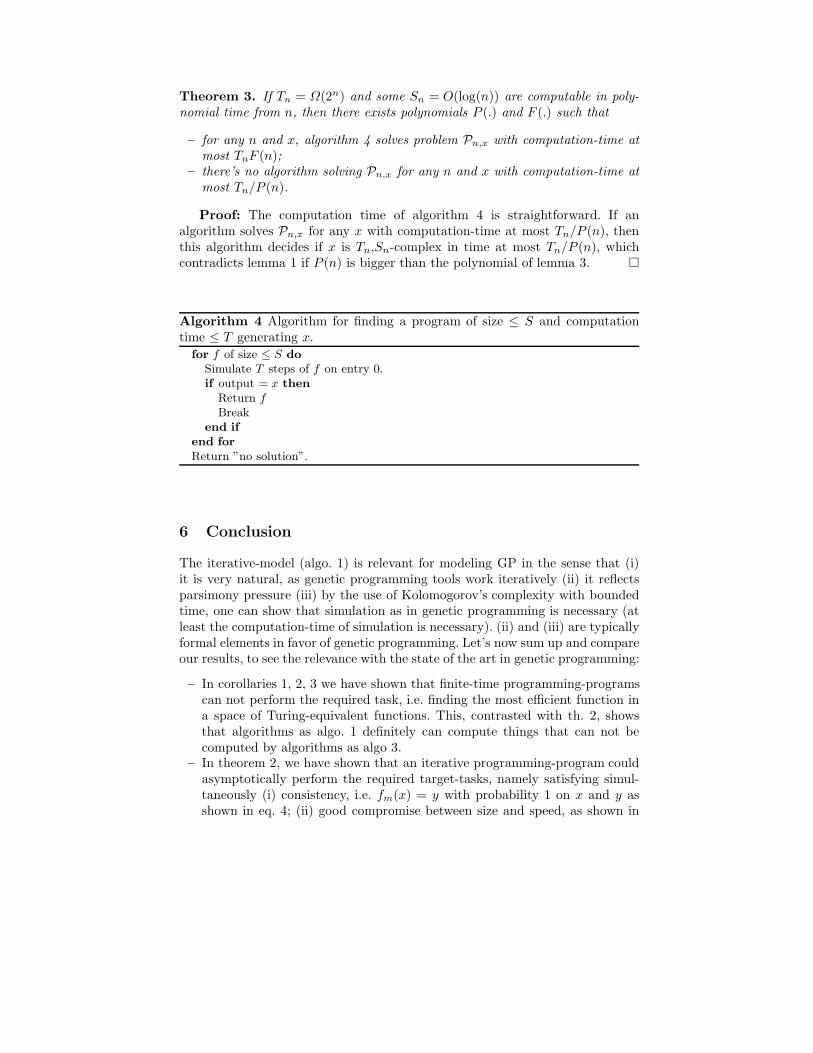
Theorem 3. If Tn = Ω(2n) and some Sn = O(log(n)) are computable in poly-nomial time from n, then there exists polynomials P (.) and F (.) such that

– for any n and x, algorithm 4 solves problem Pn,x with computation-time atmost TnF (n);

– there’s no algorithm solving Pn,x for any n and x with computation-time atmost Tn/P (n).

Proof: The computation time of algorithm 4 is straightforward. If analgorithm solves Pn,x for any x with computation-time at most Tn/P (n), thenthis algorithm decides if x is Tn,Sn-complex in time at most Tn/P (n), whichcontradicts lemma 1 if P (n) is bigger than the polynomial of lemma 3.

Algorithm 4 Algorithm for finding a program of size ≤ S and computationtime ≤ T generating x.

for f of size ≤ S do

Simulate T steps of f on entry 0.if output = x then

Return f

Breakend if

end for

Return ”no solution”.

6 Conclusion

The iterative-model (algo. 1) is relevant for modeling GP in the sense that (i)it is very natural, as genetic programming tools work iteratively (ii) it reflectsparsimony pressure (iii) by the use of Kolomogorov’s complexity with boundedtime, one can show that simulation as in genetic programming is necessary (atleast the computation-time of simulation is necessary). (ii) and (iii) are typicallyformal elements in favor of genetic programming. Let’s now sum up and compareour results, to see the relevance with the state of the art in genetic programming:

– In corollaries 1, 2, 3 we have shown that finite-time programming-programscan not perform the required task, i.e. finding the most efficient function ina space of Turing-equivalent functions. This, contrasted with th. 2, showsthat algorithms as algo. 1 definitely can compute things that can not becomputed by algorithms as algo 3.

– In theorem 2, we have shown that an iterative programming-program couldasymptotically perform the required target-tasks, namely satisfying simul-taneously (i) consistency, i.e. fm(x) = y with probability 1 on x and y asshown in eq. 4; (ii) good compromise between size and speed, as shown in

eq. 5. Interestingly, we need parsimony pressure in theorem 2 (short pro-grams are preferred); parsimony pressure is usual in GP. This is a bridgebetween mathematics and practice. This leads to the conclusion that algo.1 has definitely a larger computational power than algo. 3.

– The main drawback of GP is that GP is slow, due to huge computationalcosts, as a consequence of intensive simulations during GP-runs; but anywayone can not get rid of the computation time. In theorem 3, using a modifiedform of Kolmogorov’s complexity, we have shown that getting rid of thesimulation time is anyway not possible. This shows that the fact that f isnot directly used, but only black-box-calls to f , in algo. 1, is not a strongweakness (at least within some polynomial on the computation time).

This gives a twofold theoretical foundation to GP, showing that (i) simulation +selection as in th. 2 outperforms any algorithm of the form of algo. 3 (ii) gettingrid of the simulation time is not possible, and therefore using algo. 2 instead of1 will not “very strongly” (more than polynomially) reduce the computationalcost. Of course, this in the case of mining spaces of Turing-computable functions;in more restricted cases, with more decidability properties, the picture is verydifferent. Refining comparisons between algorithms 1, 2, 3, is for the momentessentially an empirical research in the case of Turing-computable functions,termed genetic programming. The rare mathematical papers about genetic pro-gramming focus on restricted non-Turing-computable cases, whereas the mostimpressive results concern Turing-computable functions (also in the quantumcase). This study is a step in the direction of iterative-Turing-computable mod-els as a model of GP.

References

1. Wolfgang Banzhaf and William B. Langdon. Some considerations on the reasonfor bloat. Genetic Programming and Evolvable Machines, 3(1):81–91, 2002.

2. Tobias Blickle and Lothar Thiele. Genetic programming and redundancy. InJ. Hopf, editor, Genetic Algorithms Workshop at KI-94, pages 33–38. Max-Planck-Institut fur Informatik, 1994.

3. Harry Buhrman, Lance Fortnow, and Sophie Laplante. Resource-bounded kol-mogorov complexity revisited. SIAM Journal on Computing, 2001.

4. L. Fortnow and M. Kummer. Resource-bounded instance complexity. TheoreticalComputer Science A, 161:123–140, 1996.

5. S.M. Gustafson, W. Langdon, and J. Koza. Bibliography on genetic programming.In The Collection of Computer Science Bibliographies, 2007.

6. J. D. Hamkins. Infinite time turing machines. Minds Mach., 12(4):521–539, 2002.7. A. Y. Khintchine. Sur la loi forte des grands nombres. Comptes Rendus de

l’Academie des Sciences, 186, 1928.8. A.N. Kolmogorov. Logical basis for information theory and probability theory.

IEEE trans. Inform. Theory, IT-14, 662-664, 1968.9. John R. Koza. Genetic Programming: On the Programming of Computers by Means

of Natural Selection. MIT Press, Cambridge, MA, USA, 1992.10. G. Lugosi L. Devroye, L. Gyorfi. A probabilistic theory of pattern recognition,

springer. 1997.

11. W. B. Langdon. The evolution of size in variable length representations. InICEC’98, pages 633–638. IEEE Press, 1998.

12. W. B. Langdon and R. Poli. Fitness causes bloat: Mutation. In John Koza, editor,Late Breaking Papers at GP’97, pages 132–140. Stanford Bookstore, 1997.

13. W. B. Langdon and Riccardo Poli. Foundations of Genetic Programming. Springer-Verlag, 2002.

14. W. B. Langdon, T. Soule, R. Poli, and J. A. Foster. The evolution of size andshape. In L. Spector, W. B. Langdon, U.-M. O’Reilly, and P. Angeline, editors,Advances in Genetic Programming III, pages 163–190. MIT Press, 1999.

15. William B. Langdon. Genetic Programming and Data Structures: Genetic Pro-gramming + Data Structures = Automatic Programming!, volume 1 of GeneticProgramming. Kluwer, Boston, 24 April 1998.

16. Sean Luke and Liviu Panait. Lexicographic parsimony pressure. In W. B. Langdonet al., editor, GECCO 2002: Proceedings of the Genetic and Evolutionary Compu-tation Conference, pages 829–836. Morgan Kaufmann Publishers, 2002.

17. Peter Nordin and Wolfgang Banzhaf. Complexity compression and evolution. InL. Eshelman, editor, Genetic Algorithms: Proceedings of the Sixth InternationalConference (ICGA95), pages 310–317, Pittsburgh, PA, USA, 15-19 July 1995. Mor-gan Kaufmann.

18. V. Pareto. Manuale d’Economia Politica. Milano: Societ Editrice, Libraria, 1906.19. A. Ratle and M. Sebag. Avoiding the bloat with probabilistic grammar-guided

genetic programming. In P. Collet et al., editor, Artificial Evolution VI. SpringerVerlag, 2001.

20. H. Rogers. Theory of recursive functions and effective computability. McGraw-Hill,New York, 1967.

21. J. Schmidthuber. Hierarchies of generalized kolmogorov complexities and nonenu-merable universal measures computable in the limit. International Journal ofFoundations of Computer Science 13(4):587-612, 2002.

22. Sara Silva and Jonas Almeida. Dynamic maximum tree depth : A simple techniquefor avoiding bloat in tree-based gp. In E. Cantu-Paz et al., editor, Genetic andEvolutionary Computation – GECCO-2003, volume 2724 of LNCS, pages 1776–1787. Springer-Verlag, 2003.

23. M. Sipser. A complexity theoretic approach to randomness. In Proceedings of the15th ACM Symposium on the Theory of Computing, pages 330–335, 1983.

24. Ray Solomonoff. A formal theory of inductive inference, part 1. Inform. andControl, vol. 7, number 1, pp. 1-22, 1964.

25. Ray Solomonoff. A formal theory of inductive inference, part 2. Inform. andControl, vol. 7, number 2, pp. 222-254, 1964.

26. T. Soule and J. A. Foster. Effects of code growth and parsimony pressure onpopulations in genetic programming. Evolutionary Computation, 6(4):293–309,1998.

27. Terence Soule. Exons and code growth in genetic programming. In James A. Fosteret al., editor, EuroGP 2002, volume 2278 of LNCS, pages 142–151. Springer-Verlag,2002.

28. A. Turing. On computable numbers, with an application to the entscheidungsprob-lem. proceedings of the London Mathematical Society, Ser. 2, 45, pp. 161-228(reprinted in M. Davis (1965), The Undecidable, Ewlett, NY: Raven Press, pp.155-222), 1936-1937.

29. V. Vapnik. The nature of statistical learning, springer. 1995.30. B.-T. Zhang and H. Muhlenbein. Balancing accuracy and parsimony in genetic

programming. Evolutionary Computation, vol. 3, no. 1, pp. 17-38, 1995.