slides for chapter 5 note to instructors license © 2012 john s. conery the slides in this keynote...
TRANSCRIPT

Slides for Chapter 5
Note to Instructors
License
© 2012 John S. Conery
The slides in this Keynote document are based on copyrighted material from Explorations in Computing: An Introduction to Computer Science, by John S. Conery.
These slides are provided free of charge to instructors who are using the textbook for their courses.
Instructors may alter the slides for use in their own courses, including but not limited to: adding new slides, altering the wording or images found on these slides, or deleting slides.
Instructors may distribute printed copies of the slides, either in hard copy or as electronic copies in PDF form, provided the copyright notice below is reproduced on the first slide.
This Keynote document contains the slides for “Divide and Conquer”, Chapter 5 of Explorations in Computing: An Introduction to Computer Science.
The book invites students to explore ideas in computer science through interactive tutorials where they type expressions in Ruby and immediately see the results, either in a terminal window or a 2D graphics window.
Instructors are strongly encouraged to have a Ruby session running concurrently with Keynote in order to give live demonstrations of the Ruby code shown on the slides.

Explorations in Computing
© 2012 John S. Conery
Breaking large problems into smaller subproblems
Divide and Conquer
✦ Binary Search
✦ Binary Search Experiments
✦ Merge Sort
✦ Merge Sort Experiments
✦ Recursive Methods
Iterative Searches
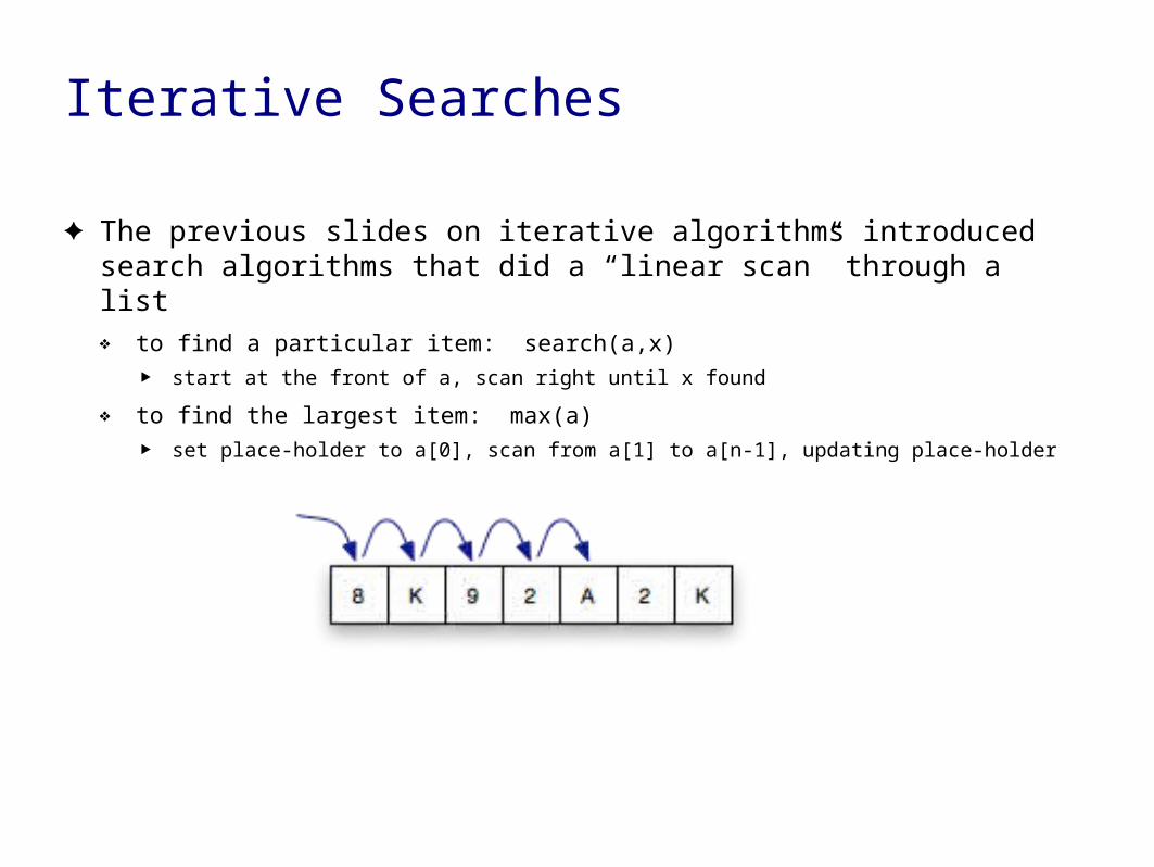
✦ The previous slides on iterative algorithms introduced search algorithms that did a “linear scan” through a list❖ to find a particular item: search(a,x)
‣ start at the front of a, scan right until x found
❖ to find the largest item: max(a)
‣ set place-holder to a[0], scan from a[1] to a[n-1], updating place-holder

Simple Sorts
✦ Those slides also introduced a sorting algorithm that used a similar strategy
✦ Scan the list from left to right, and for each item x:❖ remove x from the list
❖ scan left to find a place for x
❖ re-insert x into the list
✦ This “insertion sort” algorithm has nested loops❖ outer loop is a linear progression left to right
❖ inner loop scans back to find a place for x
✦ The number of comparisons made when sortinga list of n items is as high as
Divide and Conquer
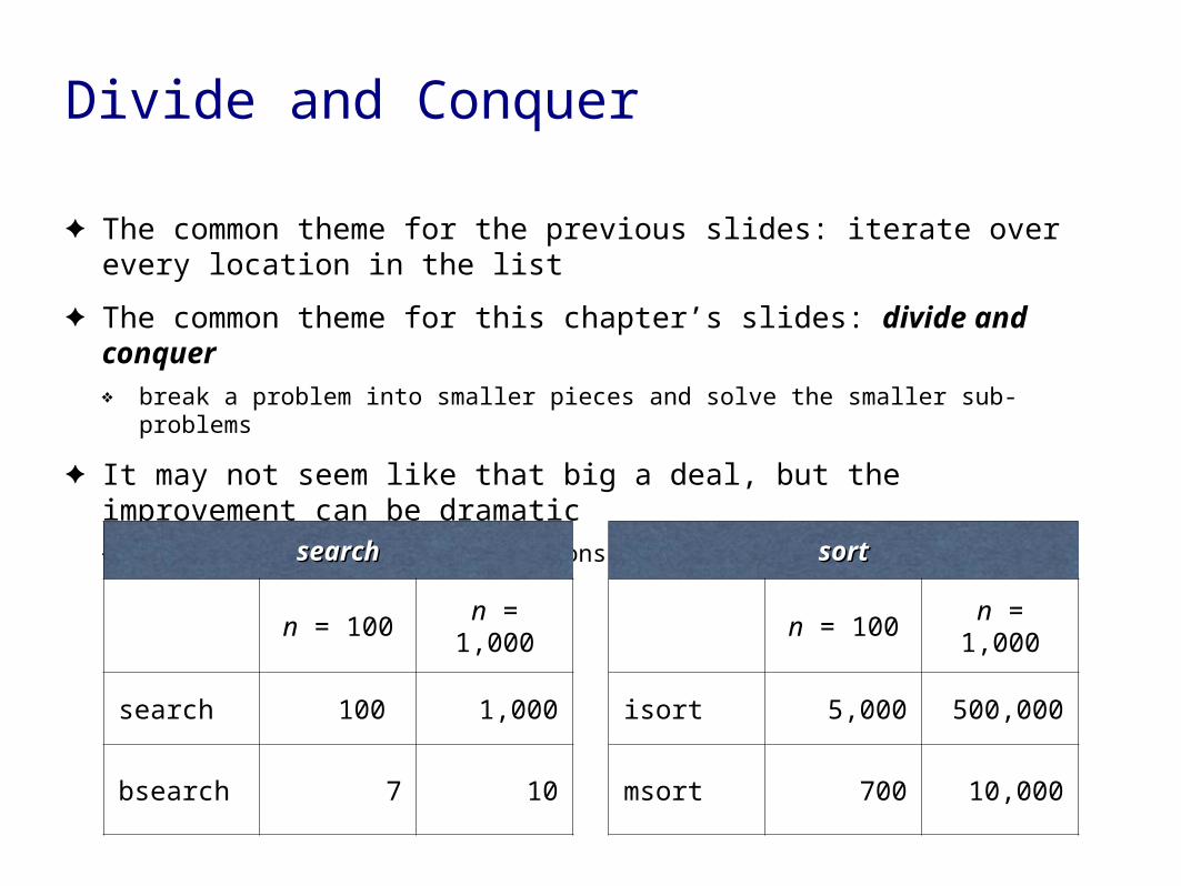
✦ The common theme for the previous slides: iterate over every location in the list
✦ The common theme for this chapter’s slides: divide and conquer❖ break a problem into smaller pieces and solve the smaller sub-problems
✦ It may not seem like that big a deal, but the improvement can be dramatic❖ approximate number of comparisons (worst case):
searchsearch
n = 100n =
1,000
search 100 1,000
bsearch 7 10
sortsort
n = 100n =
1,000
isort 5,000 500,000
msort 700 10,000

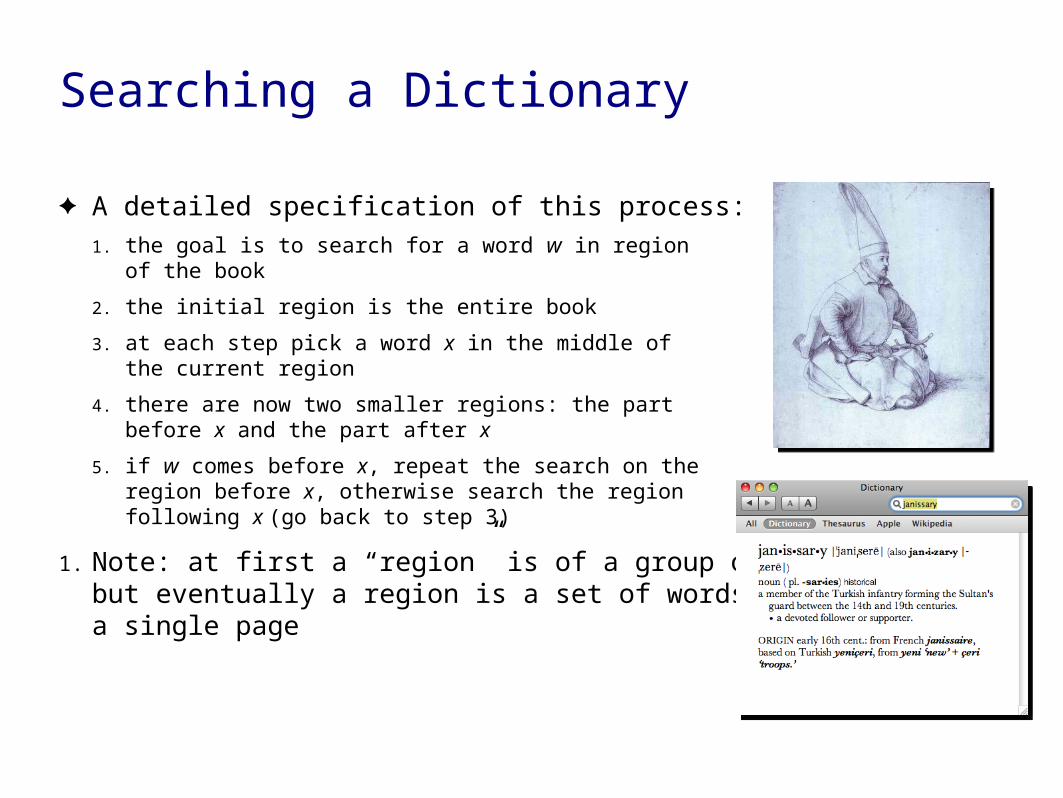
Searching a Dictionary
✦ To get a general sense of how the divideand conquer strategy improves search,consider how people find information in a phone book or dictionary❖ suppose you want to find “janissary” in
a dictionary
❖ open the book near the middle
❖ the heading on the top left page is “kiwi”, so move back a small number of pages
❖ here you find “hypotenuse”, so move forward
❖ find “ichthyology”, move forward again
✦ The number of pages you move getssmaller (or at least adjusts in responseto the words you find)
Searching a Dictionary
✦ A detailed specification of this process:
1. the goal is to search for a word w in region of the book
2. the initial region is the entire book
3. at each step pick a word x in the middle ofthe current region
4. there are now two smaller regions: the part before x and the part after x
5. if w comes before x, repeat the search on theregion before x, otherwise search the regionfollowing x (go back to step 3)
1. Note: at first a “region” is of a group of pages,but eventually a region is a set of words ona single page

A Note About Organization
✦ An important note: an efficient search depends on having the data organized in some fashion ❖ if books in a library are scattered all over the place we would have to do an iterative search
❖ start at one end of the room and progress toward the other
✦ If books are sorted or carefully cataloged we can try a binary search or other method
http://www.endlessbookshelf.net/shelves.html
Binary Search
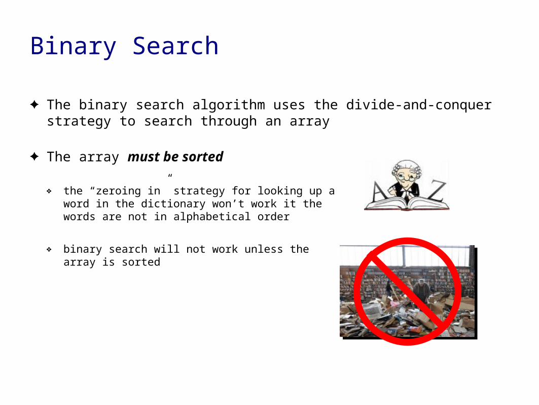
✦ The binary search algorithm uses the divide-and-conquer strategy to search through an array
✦ The array must be sorted
❖ the “zeroing in” strategy for looking up aword in the dictionary won’t work it thewords are not in alphabetical order
❖ binary search will not work unless thearray is sorted
Binary Search
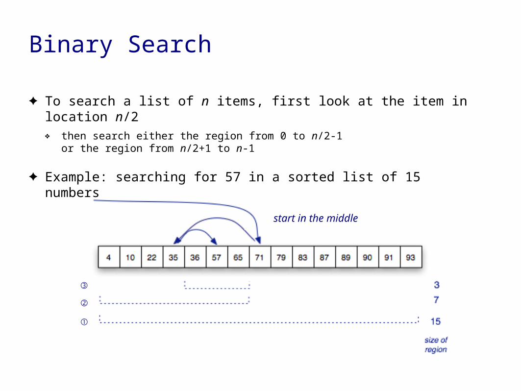
✦ To search a list of n items, first look at the item in location n/2❖ then search either the region from 0 to n/2-1
or the region from n/2+1 to n-1
✦ Example: searching for 57 in a sorted list of 15 numbers
①
②
③
start in the middle

Detailed Description
✦ The algorithm uses two variables to keep track of the boundaries of the region to search
lower the index one below the leftmost item in the region
upper the index one above the rightmost region
[ ]
initial values when searching an array of n items:lower = -1
upper = n
Detailed Description
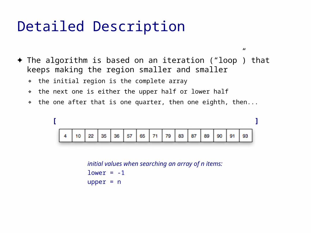
✦ The algorithm is based on an iteration (“loop”) that keeps making the region smaller and smaller❖ the initial region is the complete array
❖ the next one is either the upper half or lower half
❖ the one after that is one quarter, then one eighth, then...
[ ]
initial values when searching an array of n items:lower = -1
upper = n
Detailed Description
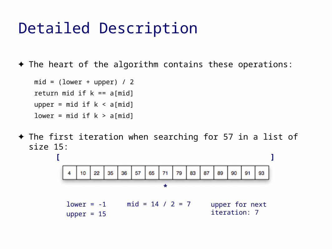
✦ The heart of the algorithm contains these operations:
mid = (lower + upper) / 2
return mid if k == a[mid]
upper = mid if k < a[mid]
lower = mid if k > a[mid]
✦ The first iteration when searching for 57 in a list of size 15:
[ ]
lower = -1
upper = 15
mid = 14 / 2 = 7
*
upper for next iteration: 7

Detailed Description
✦ The remaining iterations whensearching for 57:
lower = -1upper = 7mid = 3lower = 3
lower = 3upper = 7mid = 5found it!
[ ]
[ ]
*
*
This search required only 3 comparisons:
a[7], a[3], a[5]
mid = (lower + upper) / 2return mid if k == a[mid]upper = mid if k < a[mid]lower = mid if k > a[mid]
mid = (lower + upper) / 2return mid if k == a[mid]upper = mid if k < a[mid]lower = mid if k > a[mid]

Unsuccessful Searches
✦ What happens in this algorithmif the item we’re looking foris not in the array?
✦ Example: search for 58
lower = 3upper = 7mid = 5lower = 5
lower = 5upper = 7mid = 6upper = 6
lower = 5upper = 6mid = 5lower = 5
mid = (lower + upper) / 2return mid if k == a[mid]upper = mid if k < a[mid]lower = mid if k > a[mid]
mid = (lower + upper) / 2return mid if k == a[mid]upper = mid if k < a[mid]lower = mid if k > a[mid]
[ ]*
[ ]*
[ ]
uh-oh... lower
didn’t change!
Unsuccessful Searches
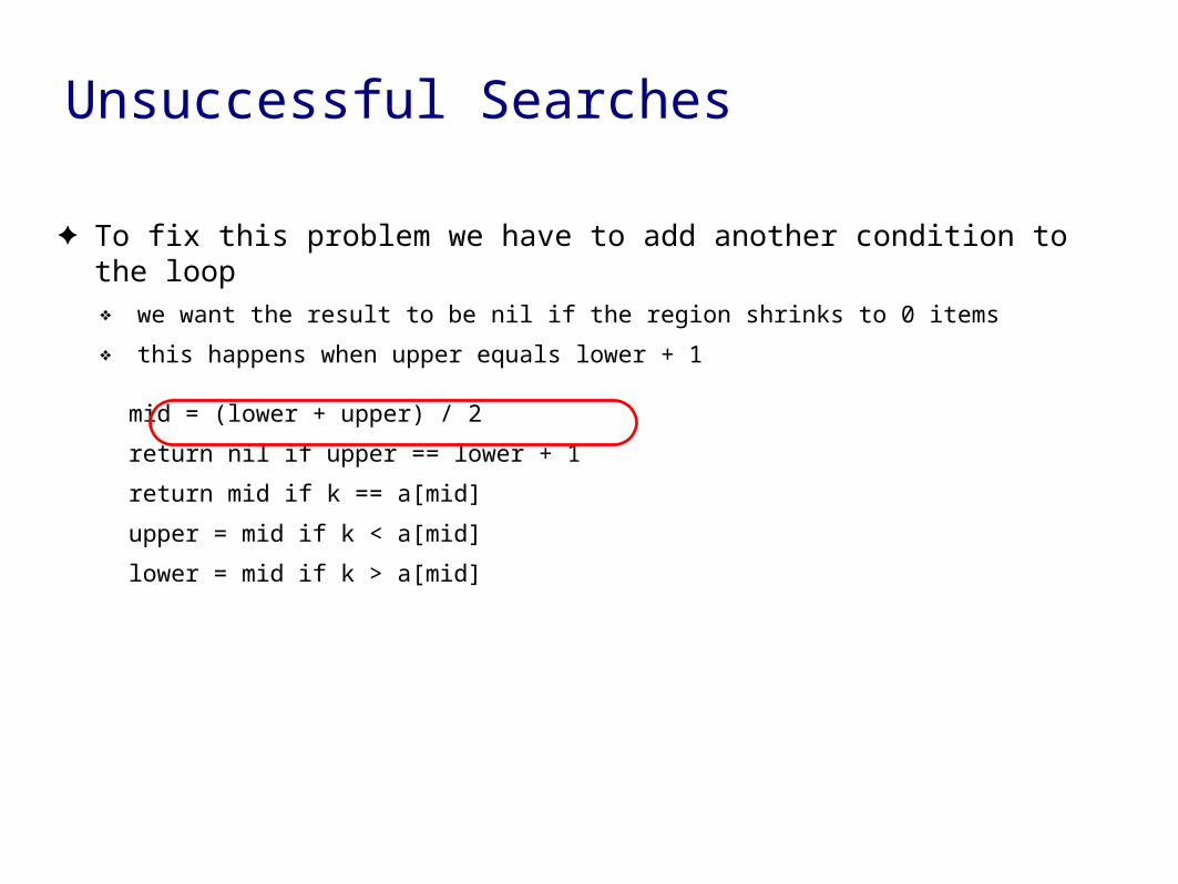
✦ To fix this problem we have to add another condition to the loop❖ we want the result to be nil if the region shrinks to 0 items
❖ this happens when upper equals lower + 1
mid = (lower + upper) / 2
return nil if upper == lower + 1
return mid if k == a[mid]
upper = mid if k < a[mid]
lower = mid if k > a[mid]

if Statements
✦ Usually when a program has tests for opposite conditions the test is written in the form of an if statement
✦ Instead of
upper = mid if k < a[mid]
lower = mid if k > a[mid]
we normally write
if k < a[mid]
upper = mid
else
lower = mid
end
if and else are keywords

if Statements
✦ If there are three conditions we can use elsif (a combination of if and else):
if k == a[mid]
return mid
elsif k < a[mid]
upper = mid
else
lower = mid
end
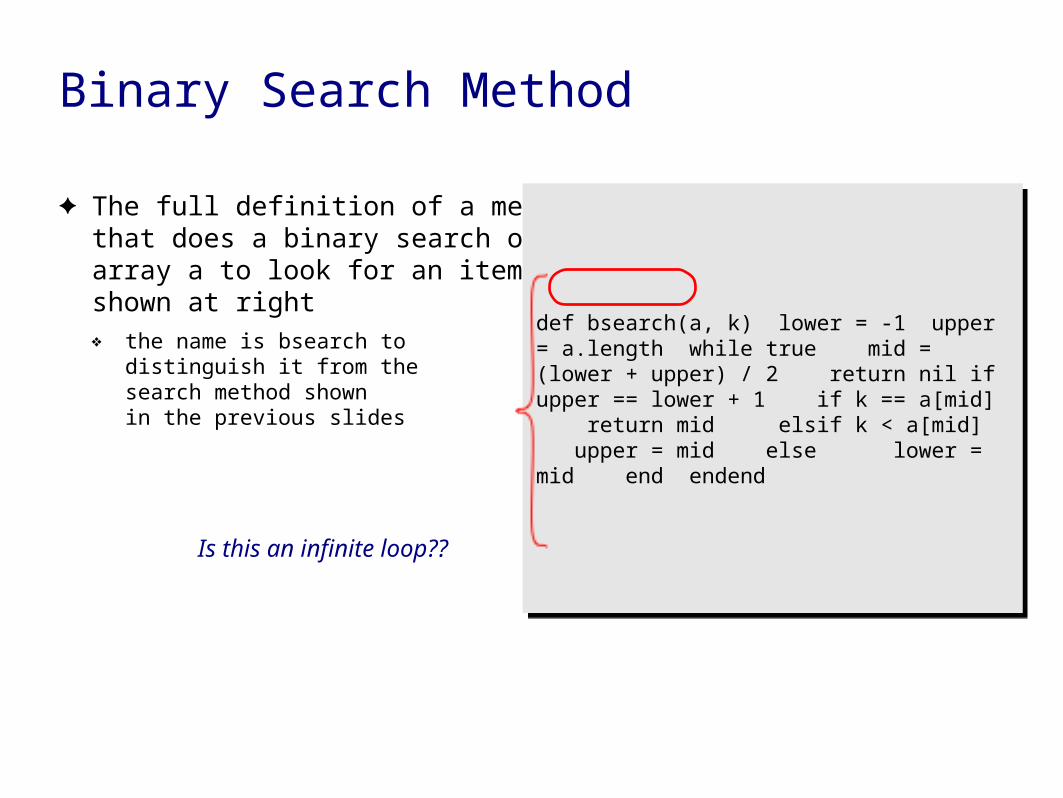
Binary Search Method
✦ The full definition of a method that does a binary search of an array a to look for an item x is shown at right❖ the name is bsearch to
distinguish it from the search method shownin the previous slides
def bsearch(a, k) lower = -1 upper = a.length while true mid = (lower + upper) / 2 return nil if upper == lower + 1 if k == a[mid] return mid elsif k < a[mid] upper = mid else lower = mid end endend
def bsearch(a, k) lower = -1 upper = a.length while true mid = (lower + upper) / 2 return nil if upper == lower + 1 if k == a[mid] return mid elsif k < a[mid] upper = mid else lower = mid end endend
Is this an infinite loop??

Examples with bsearch
✦ The bsearch method is part of a module named RecursionLab
>> include RecursionLab
=> Object
>> a = TestArray.new(15).sort
=> [2, 8, 10, 25, 28, 29, 40, 43, 54, 55, 59, 68, 88, 90, 91]
>> bsearch(a, 10)
=> 2
>> bsearch(a, 42)
=> nil
Make sure the array to search is sorted!

Experiments with bsearch
✦ The brackets method used to monitor the progress of search and isort can also be used here
>> a = TestArray.new(7).sort
=> [8, 12, 18, 20, 32, 34, 36]
>> puts brackets(a,0)
[8 12 18 20 32 34 36]
>> puts brackets(a,0,2)
[8 12 18] 20 32 34 36
>> puts brackets(a,0,2,1)
[8 *12 18] 20 32 34 36
print bracket before a[0]
print bracket before a[0], after a[2]
as above, but include a * at a[1]

Experiments with bsearch (cont’d)
✦ Print a listing of the method to find a line number to attach a probe:
>> Source.listing("bsearch")
...
4: while true
5: mid = (lower + upper) / 2
6: return nil if upper == lower + 1
7: return mid if k == a[mid]
...
✦ The goal is to count the number of iterations❖any statement inside the loop will do
❖but display is more informative if we probe line 6, after computing mid
★
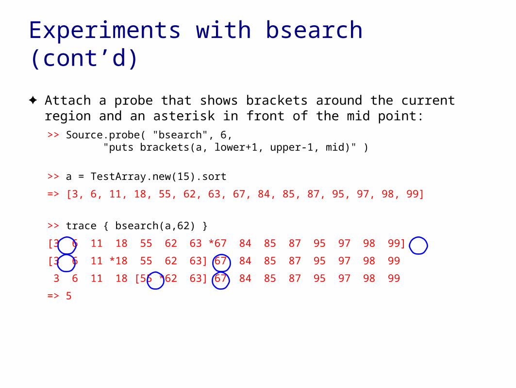
Experiments with bsearch (cont’d)
✦ Attach a probe that shows brackets around the current region and an asterisk in front of the mid point:
>> Source.probe( "bsearch", 6, "puts brackets(a, lower+1, upper-1, mid)" )
>> a = TestArray.new(15).sort
=> [3, 6, 11, 18, 55, 62, 63, 67, 84, 85, 87, 95, 97, 98, 99]
>> trace { bsearch(a,62) }
[3 6 11 18 55 62 63 *67 84 85 87 95 97 98 99]
[3 6 11 *18 55 62 63] 67 84 85 87 95 97 98 99
3 6 11 18 [55 *62 63] 67 84 85 87 95 97 98 99
=> 5

Experiments with bsearch (cont’d)
✦ Here is a trace of an unsuccessful search:
>> a = TestArray.new(15).sort
=> [2, 9, 12, 13, 14, 20, 36, 54, 67, 70, 75, 78, 91, 92, 96]
>> x = a.random(:fail)
=> 88
>> trace { bsearch(a,x) }
[2 9 12 13 14 20 36 *54 67 70 75 78 91 92 96]
2 9 12 13 14 20 36 54 [67 70 75 *78 91 92 96]
2 9 12 13 14 20 36 54 67 70 75 78 [91 *92 96]
2 9 12 13 14 20 36 54 67 70 75 78 [91] 92 96
2 9 12 13 14 20 36 54 67 70 75 78 [] 91 92 96
=> nil
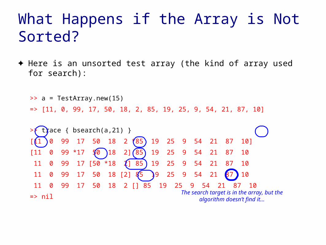
What Happens if the Array is Not Sorted?
✦ Here is an unsorted test array (the kind of array used for search):
>> a = TestArray.new(15)
=> [11, 0, 99, 17, 50, 18, 2, 85, 19, 25, 9, 54, 21, 87, 10]
>> trace { bsearch(a,21) }
[11 0 99 17 50 18 2 *85 19 25 9 54 21 87 10]
[11 0 99 *17 50 18 2] 85 19 25 9 54 21 87 10
11 0 99 17 [50 *18 2] 85 19 25 9 54 21 87 10
11 0 99 17 50 18 [2] 85 19 25 9 54 21 87 10
11 0 99 17 50 18 2 [] 85 19 25 9 54 21 87 10
=> nilThe search target is in the array, but the
algorithm doesn’t find it...

Cutting the Problem Down to Size
✦ It should be clear why we say the binary search uses a divide and conquer strategy❖ the problem is to find an item within a given range
‣ initial range: entire array
❖ at each step the problem is split into two equal sub-problems
❖ focus turns to one sub-problem for the next step
* = value of mid on each iterationin a search for 57
*
*
*
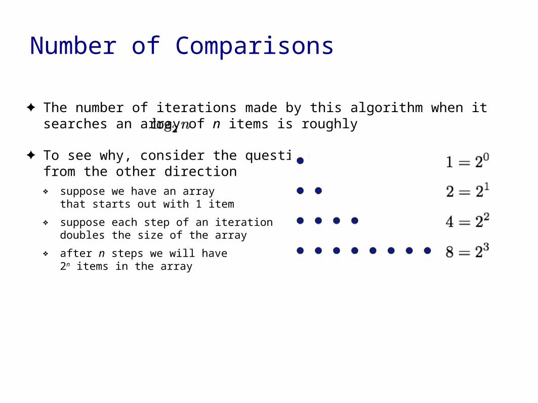
Number of Comparisons
✦ The number of iterations made by this algorithm when it searches an array of n items is roughly
✦ To see why, consider the question from the other direction❖ suppose we have an array
that starts out with 1 item
❖ suppose each step of an iteration doubles the size of the array
❖ after n steps we will have 2n items in the array
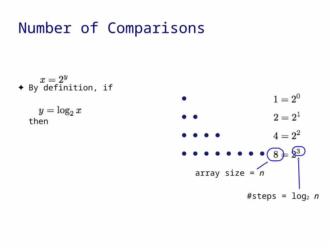
Number of Comparisons
✦ By definition, if
then
array size = n
#steps = log2 n

Number of Comparisons
✦ When we’re searching we’rereducing an area of size n downto an area of size 1
e.g. n = 8 in this diagram
✦ A successful search might returnafter the first comparison
✦ An unsuccessful search doesall iterations
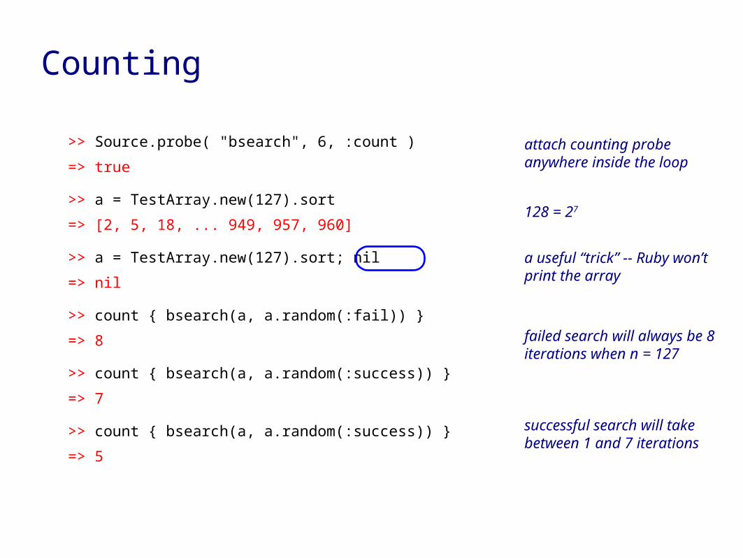
Counting
>> Source.probe( "bsearch", 6, :count )
=> true
>> a = TestArray.new(127).sort
=> [2, 5, 18, ... 949, 957, 960]
>> a = TestArray.new(127).sort; nil
=> nil
>> count { bsearch(a, a.random(:fail)) }
=> 8
>> count { bsearch(a, a.random(:success)) }
=> 7
>> count { bsearch(a, a.random(:success)) }
=> 5
attach counting probeanywhere inside the loop
128 = 27
a useful “trick” -- Ruby won’t print the array
failed search will always be 8 iterations when n = 127
successful search will take between 1 and 7 iterations
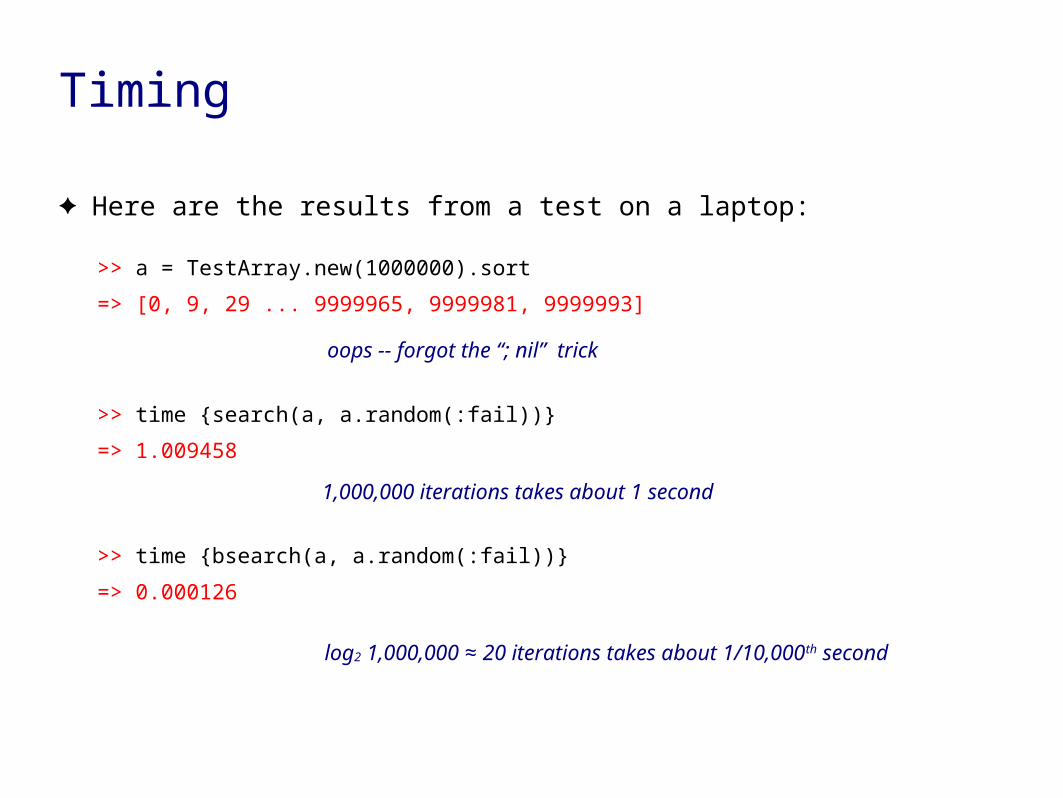
Timing
✦ Here are the results from a test on a laptop:
>> a = TestArray.new(1000000).sort
=> [0, 9, 29 ... 9999965, 9999981, 9999993]
>> time {search(a, a.random(:fail))}
=> 1.009458
>> time {bsearch(a, a.random(:fail))}
=> 0.000126
oops -- forgot the “; nil” trick
1,000,000 iterations takes about 1 second
log2 1,000,000 ≈ 20 iterations takes about 1/10,000th second

Recursion
✦ In computer science a recursive description of a problem is one where❖ a problem can be broken into smaller parts
❖ each part is a smaller version of the original problem
❖ there is a “base case” that can be solved immediately (i.e. it has no sub-problems)
✦ Binary search can be described recursively:
search(a, k, lower, upper):
mid = (lower + upper) / 2
return nil if mid == lower
return mid if k == a[mid]
return search(a, k, lower, mid) if k < a[mid]
return search(a, k, mid, upper) if k > a[mid]
base cases -- no further breakdown required
recursion-- smaller instances of the original problem
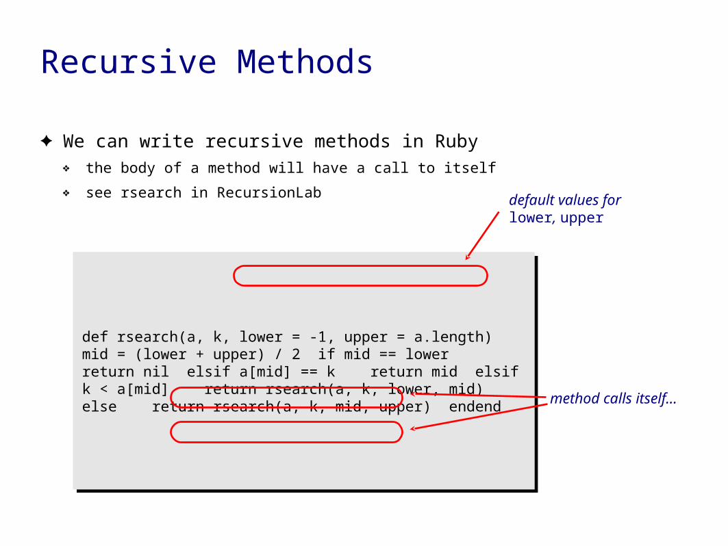
Recursive Methods
✦ We can write recursive methods in Ruby❖ the body of a method will have a call to itself
❖ see rsearch in RecursionLab
def rsearch(a, k, lower = -1, upper = a.length) mid = (lower + upper) / 2 if mid == lower return nil elsif a[mid] == k return mid elsif k < a[mid] return rsearch(a, k, lower, mid) else return rsearch(a, k, mid, upper) endend
def rsearch(a, k, lower = -1, upper = a.length) mid = (lower + upper) / 2 if mid == lower return nil elsif a[mid] == k return mid elsif k < a[mid] return rsearch(a, k, lower, mid) else return rsearch(a, k, mid, upper) endend
default values for lower, upper
method calls itself...

Recursive Methods (cont’d)
>> rsearch(a, 29)
[ 12 19 29 *58 68 72 96 98 ]
[ 12 *19 29 ] 58 68 72 96 98
12 19 [ *29 ] 58 68 72 96 98
=> 2
def rsearch(a, k, lower = -1, upper = a.length) mid = (lower + upper) / 2 if mid == lower return nil elsif a[mid] == k return mid elsif k < a[mid] return rsearch(a, k, lower, mid) else return rsearch(a, k, mid, upper) endend
def rsearch(a, k, lower = -1, upper = a.length) mid = (lower + upper) / 2 if mid == lower return nil elsif a[mid] == k return mid elsif k < a[mid] return rsearch(a, k, lower, mid) else return rsearch(a, k, mid, upper) endend
recursive call, lower = -1, upper = 3
recursive call, lower = 1, upper = 3
location where 29 was found
initial call, lower = -1, upper = 8

Recursion (cont’d)
✦ Understanding recursive methods takes some getting used to❖ it’s easy to get lost, especially if you mentally trace what the system is doing
✦ It’s a powerful tool as part of a programmer’s “toolbox”❖ many complex problems are much easier to solve when one realizes there is a recursive
description
✦ Key points to remember about recursion:❖ a recursive problem is one that can be broken into pieces
❖ each piece is a smaller instance of the original problem
❖ a recursive method calls itself to solve one of the smaller subproblems
❖ there must be a base case, otherwise the result is an infinite recursion

Divide and Conquer Sorting Algorithms
✦ The divide and conquer strategy used to make a more efficient search algorithm can also be applied to sorting
✦ Two well-known sorting algorithms:
QuickSort❖ divide a list into big values and small values, then sort each part
Merge Sort❖ sort subgroups of size 2, merge them into sorted groups of size 4, merge those into sorted
groups of size 8, ...
✦ The remaining slides will have an overview of each algorithm, and a look at how Merge Sort can be implemented in Ruby

Merge Sort
✦ The merge sort algorithm works from “the bottom up”❖ start by solving the smallest pieces of the main problem
❖ keep combining their results into larger solutions
❖ eventually the original problem will be solved
✦ Example: sorting playing cards❖ divide the cards into groups of two
❖ sort each group -- put the smaller of the two on the top
❖ merge groups of two into groups of four
❖ merge groups of four into groups of eight
❖ ...
[ see example next slide ]
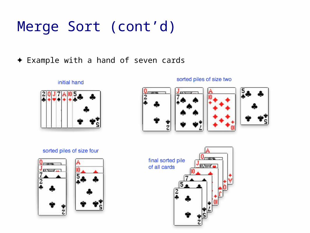
Merge Sort (cont’d)
✦ Example with a hand of seven cards

Merge Sort
✦ What makes this method moreeffective than simple insertion sort?❖ merging two piles is a very simple
operation
❖ only need to look at the two cardscurrently on the top of each pile
❖ no need to look deeper into eithergroup
✦ In this example:❖ compare 2 with 5, pick up the 2
❖ compare 5 with 7, pick up the 5
❖ compare 7 with 10, pick up the 7
❖ ....

Merge Sort
✦ Another example, using an array of numbers❖ sorted blocks are indicated by adjacent cells with the same color
msort Demo
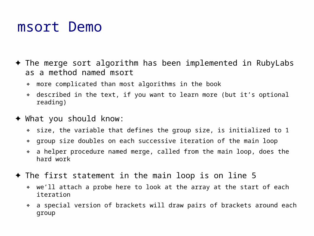
✦ The merge sort algorithm has been implemented in RubyLabs as a method named msort❖ more complicated than most algorithms in the book
❖ described in the text, if you want to learn more (but it’s optional reading)
✦ What you should know:❖ size, the variable that defines the group size, is initialized to 1
❖ group size doubles on each successive iteration of the main loop
❖ a helper procedure named merge, called from the main loop, does the hard work
✦ The first statement in the main loop is on line 5❖ we’ll attach a probe here to look at the array at the start of each iteration
❖ a special version of brackets will draw pairs of brackets around each group

msort Demo
✦ An example of how to call msort_brackets
>> a = TestArray.new(8)
=> [38, 45, 24, 13, 52, 25, 48, 26]
>> puts msort_brackets(a, 2)
[38 45] [24 13] [52 25] [48 26]
>> puts msort_brackets(a, 4)
[38 45 24 13] [52 25 48 26]
>> Source.probe( "msort", 5, "puts msort_brackets(a,size)" )
=> true

msort Demo
✦ After attaching the probe we can trace a call to msort
>> a = TestArray.new(16)
=> [60, 83, 6, 89, 67, 56, 40, 68, 13, 52, 96, 41, 25, 64, 37, 59]
>> trace { msort(a) }
[60] [83] [6] [89] [67] [56] [40] [68] [13] [52] [96] [41] [25] [64] [37] [59]
[60 83] [6 89] [56 67] [40 68] [13 52] [41 96] [25 64] [37 59]
[6 60 83 89] [40 56 67 68] [13 41 52 96] [25 37 59 64]
[6 40 56 60 67 68 83 89] [13 25 37 41 52 59 64 96]
=> [6, 13, 25, 37, 40, 41, 52, 56, 59, 60, 64, 67, 68, 83, 89, 96]

Comparisons in Merge Sort
✦ To completely sort an array with n items requires log2 n iterations❖ the group size starts at 1 and
doubles on each iteration
✦ During each iteration there areat most n comparisons❖ comparisons occur in the
merge method
❖ compare values at the front of each group
❖ may have to work all the wayto the end of each group, but might stop early (e.g. with cardsone pile is emptied but morethan one left in the other pile)
Total comparisons ≈

Scalability of Merge Sort
✦ Is this new formula that muchbetter than thecomparisons made by isort?
❖ not that big of a differencefor small arrays
>> a = TestArray.new(10)
=> [22, 44, 51, ... ]
>> count { isort(a) }
=> 36
>> count { msort(a) }
=> 23
Note: both methods use less; attach counting probe to line 2 of less

Scalability of Merge Sort (cont’d)
✦ But for larger arrays the differenceis clear
>> a = TestArray.new(1000)
>> count { isort(a) }
=> 250770
>> count { msort(a) }
=> 8743
>> time { isort(a) }
=> 0.790905
>> time { msort(a) }
=> 0.057595
Warning: methods are a lot slower when called via trace or count

QuickSort
✦ QuickSort is another divide-and-conquer sorting algorithm
✦ The main idea is to partition the array into two regions:❖ small items are moved to the left side of the array
❖ large items are moved to the right side
✦ After partitioning, repeat the sort on the left and right sides❖ each region is a sub-problem, a smaller version of the original problem
✦ Main question: how do we decide which items are “small” and which are “large”?
✦ A common technique: use the first item in the region as a pivot❖ everything less than the pivot ends up in the left region
❖ items greater than or equal to the pivot go in the right region

Partition Example
The partitioning algorithm works from both ends
When it finds a large item on the left and a small item on the right it swaps them
When there are no more exchanges to make the two regions are complete
Numbers below 79Numbers 79 and above
QuickSort Algorithm
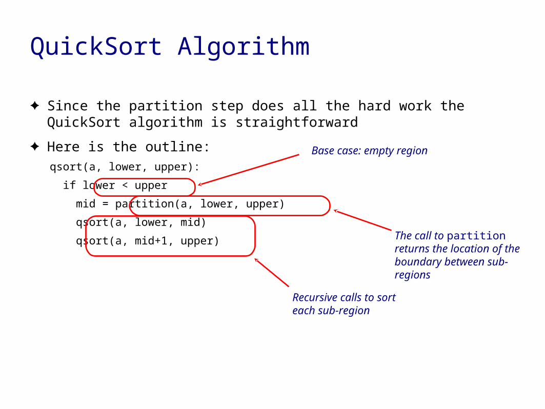
✦ Since the partition step does all the hard work the QuickSort algorithm is straightforward
✦ Here is the outline:
qsort(a, lower, upper):
if lower < upper
mid = partition(a, lower, upper)
qsort(a, lower, mid)
qsort(a, mid+1, upper) The call to partition returns the location of the boundary between sub-regions
Recursive calls to sort each sub-region
Base case: empty region
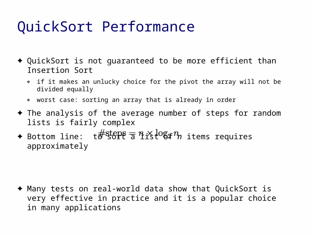
QuickSort Performance
✦ QuickSort is not guaranteed to be more efficient than Insertion Sort❖ if it makes an unlucky choice for the pivot the array will not be divided equally
❖ worst case: sorting an array that is already in order
✦ The analysis of the average number of steps for random lists is fairly complex
✦ Bottom line: to sort a list of n items requires approximately
✦ Many tests on real-world data show that QuickSort is very effective in practice and it is a popular choice in many applications

The qsort Method
✦ The RecursionLab module has a method named qsort❖ use it the same way you do isort and msort
>> Source.listing("qsort")
1: def qsort(a, p = 0, r = a.length-1)
2: if p < r
...
✦ To trace the execution of qsort, print brackets around the current region at the beginning of each call❖ parameters p and r define the boundaries
>> Source.probe( "qsort", 2, "puts brackets(a,p,r)" )
=> true
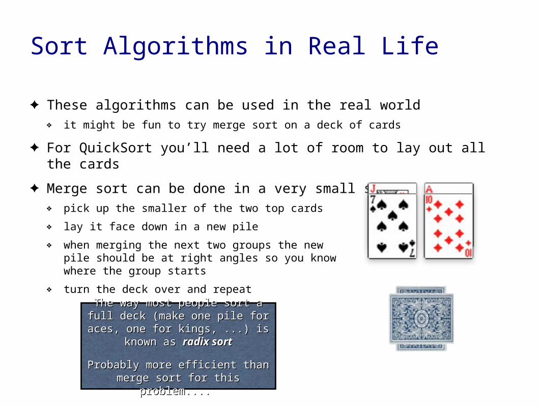
Sort Algorithms in Real Life
✦ These algorithms can be used in the real world❖ it might be fun to try merge sort on a deck of cards
✦ For QuickSort you’ll need a lot of room to lay out all the cards
✦ Merge sort can be done in a very small space❖ pick up the smaller of the two top cards
❖ lay it face down in a new pile
❖ when merging the next two groups the newpile should be at right angles so you knowwhere the group starts
❖ turn the deck over and repeat
The way most people sort a full The way most people sort a full deck (make one pile for aces, one deck (make one pile for aces, one
for kings, ...) is known as for kings, ...) is known as radix radix sortsort
Probably more efficient than merge Probably more efficient than merge sort for this problem.... sort for this problem....
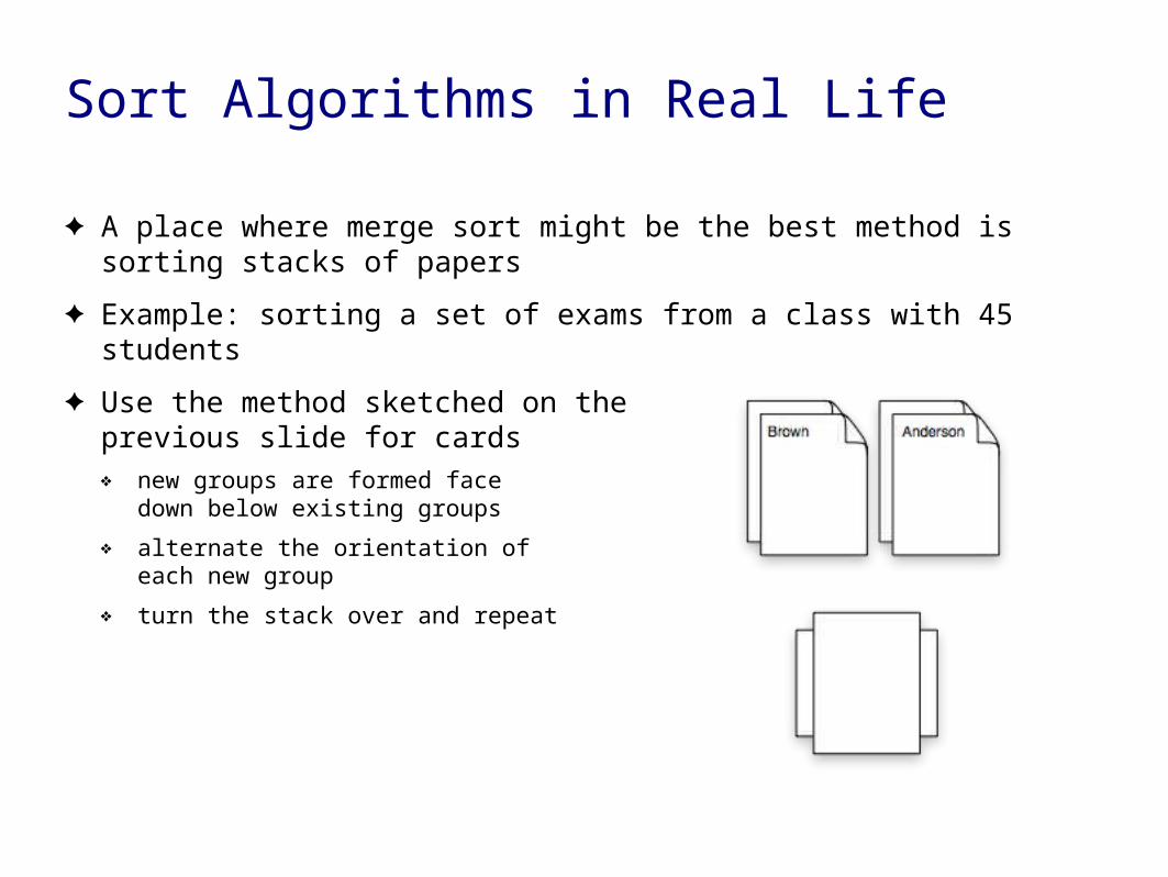
Sort Algorithms in Real Life
✦ A place where merge sort might be the best method is sorting stacks of papers
✦ Example: sorting a set of exams from a class with 45 students
✦ Use the method sketched on the previous slide for cards❖ new groups are formed face
down below existing groups
❖ alternate the orientation of each new group
❖ turn the stack over and repeat

Recap: Divide and Conquer Algorithms
✦ The divide and conquer strategy often reduces the number of iterations of the main loop from n to log2 n
❖ binary search:
❖ merge sort:
❖ QuickSort:
✦ It may not look like much, but the reduction in the number of iterations is significant for larger problems

Summary
✦ These slides introduced the divide and conquer strategy❖ for searching: binary search
‣ requires list to be sorted
❖ for sorting: QuickSort and merge sort
✦ Binary search will find an item using at most comparisons
✦ QuickSort and merge sort do at most comparisons
✦ An algorithm that uses divide and conquer can be written using iteration or recursion❖ recursive = “self-similar”
❖ a problem that can be divided into smaller subproblems of the same type
❖ a recursive method calls itself