slides -1 tp
TRANSCRIPT

8/9/2019 SLides -1 TP
http://slidepdf.com/reader/full/slides-1-tp 1/112
Transport PhenomenaMass Transfer
(1 Credit Hour)
Dr. Muhammad Rashid UsmanAssociate professor
Institute of Chemical Engineering and Technology
University of the Punjab, Lahore.
09-Sep-2014
μ α k ν D AB U i U o U D
hi ho Pr f Gr Re Le
Nu Sh Pe Sc k c K c d
Δ ρ Σ Π ∂ ∫ ∇
8/9/2019 SLides -1 TP
http://slidepdf.com/reader/full/slides-1-tp 2/112
2
The Text Book
Bird, R.B. Stewart, W.E. and Lightfoot, E.N. (2002). TransportPhenomena. 2nd ed. John Wiley & Sons, Inc. Singapore.
Please readthrough.
8/9/2019 SLides -1 TP
http://slidepdf.com/reader/full/slides-1-tp 3/112
3
Transfer processes
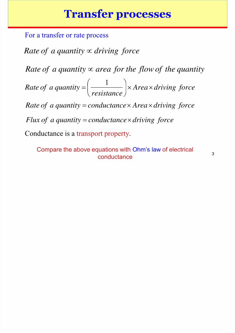
For a transfer or rate process
Conductance is a transport property.
forcedrivingquantityaof Rate ∝
forcedriving Arearesistance
quantityaof Rate ××
=
1
forcedriving Areaonductancecquantityaof Rate ××=
Compare the above equations with Ohm’s law of electrical
conductance
quantitytheof flowthe for reaaquantityaof Rate ∝
forcedrivingonductancecquantityaof luxF ×=

8/9/2019 SLides -1 TP
http://slidepdf.com/reader/full/slides-1-tp 4/112
4
Transfer processes
quantitytheof flow for area
quantitytheof ratequantityaof Flux =
timeinchange
quanitytheinchangequantityaof ate R =
distanceinchangequanitytheinchangequantityaof radient G =

8/9/2019 SLides -1 TP
http://slidepdf.com/reader/full/slides-1-tp 5/112
5
Transfer processes
In chemical engineering, we study three transfer processes (rate processes), namely
•Momentum transfer or Fluid flow
•Heat transfer
•Mass transfer
The study of these three processes is called astransport phenomena.

8/9/2019 SLides -1 TP
http://slidepdf.com/reader/full/slides-1-tp 6/112
6
Transfer processes
Transfer processes are either:• Molecular (rate of transfer is only a function
of molecular activity), or
• Convective (rate of transfer is mainly due tofluid motion or convective currents)
Unlike momentum and mass transfer processes,heat transfer has an added mode of transfer
called as radiation heat transfer.

8/9/2019 SLides -1 TP
http://slidepdf.com/reader/full/slides-1-tp 7/112
7
Summary of transfer processes
Rate Process Driving force Conductance
(Transport property)
Law for molecular
transfer
Momentumtransfer
Velocity gradient Viscosity
(Kinematic viscosity) Newton’s law of
viscosity
Heat transfer Temperature
gradient Thermal conductivity(Thermal diffusivity)
Fourier ’s law
Mass transfer Concentration
gradient (chemical potential gradient)
Mass diffusivity Fick ’s law

8/9/2019 SLides -1 TP
http://slidepdf.com/reader/full/slides-1-tp 8/112
8
Molecular rate laws
Newton’s law ofviscosity (modified)
Fourier’s law ofconduction heat transfer(modified)
Fick’s law of moleculardiffusion
8/9/2019 SLides -1 TP
http://slidepdf.com/reader/full/slides-1-tp 9/112
9
Molecular rate laws
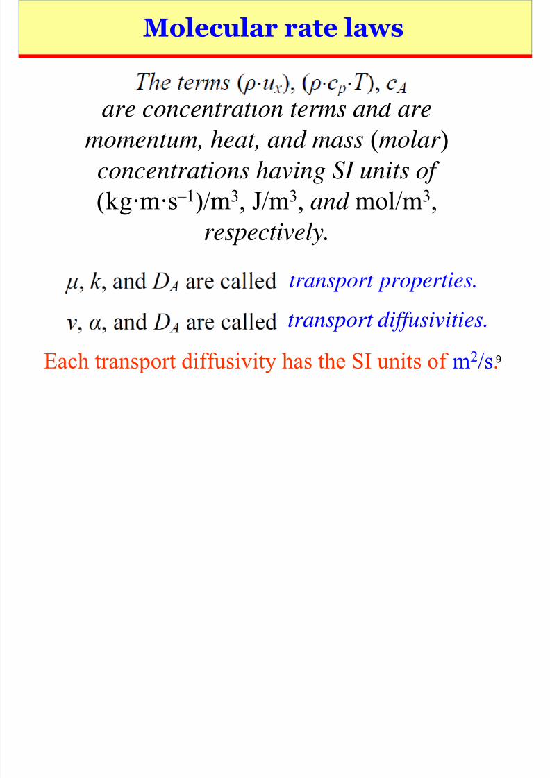
Each transport diffusivity has the SI units of m2/s.
are concentration terms and are
momentum, heat, and mass (molar )
concentrations having SI units of(kg·m·s ‒1)/m3, J/m3, and mol/m3,respectively.
transport properties.
transport diffusivities.
8/9/2019 SLides -1 TP
http://slidepdf.com/reader/full/slides-1-tp 10/112
10
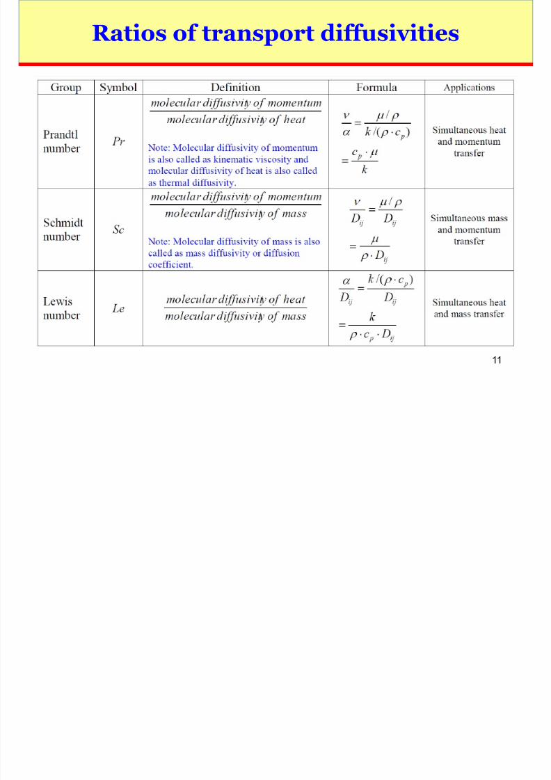
Ratios of transport diffusivities
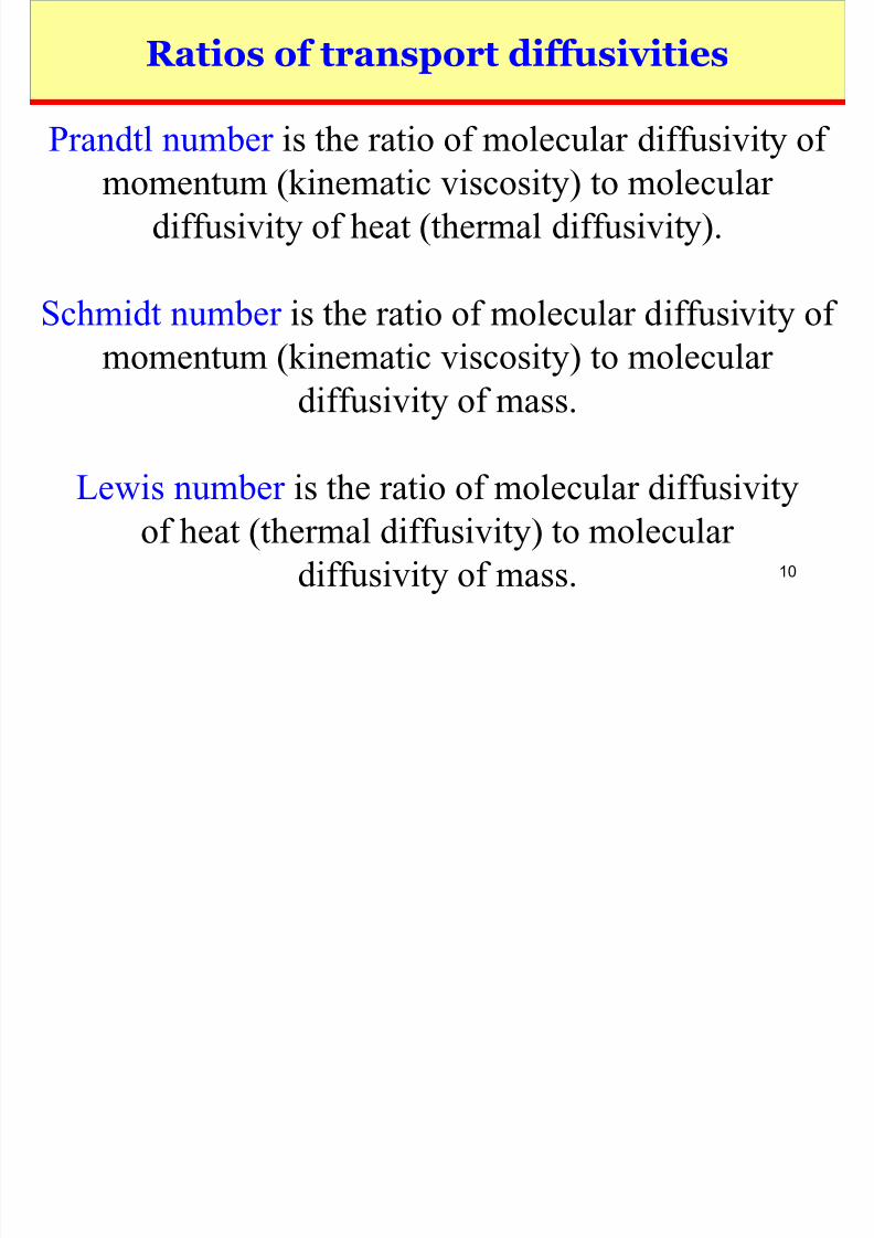
Prandtl number is the ratio of molecular diffusivity ofmomentum (kinematic viscosity) to molecular
diffusivity of heat (thermal diffusivity).
Schmidt number is the ratio of molecular diffusivity ofmomentum (kinematic viscosity) to molecular
diffusivity of mass.
Lewis number is the ratio of molecular diffusivityof heat (thermal diffusivity) to molecular
diffusivity of mass.
8/9/2019 SLides -1 TP
http://slidepdf.com/reader/full/slides-1-tp 11/112
11
Ratios of transport diffusivities

8/9/2019 SLides -1 TP
http://slidepdf.com/reader/full/slides-1-tp 12/112
12
Rapid and brief introduction to masstransfer
Mass transfer is basically of two types
•Molecular mass transfer
•Convective mass transfer
Mass transfer can be within a single phase(homogeneous) or between phases. In the lattercase it is called as “interphase mass transfer ”.

8/9/2019 SLides -1 TP
http://slidepdf.com/reader/full/slides-1-tp 13/112
13
Rapid and brief introduction to masstransfer
Fick’s Law of mass transfer
A more general driving force is based on chemical potential gradient ( μc)
dz
dc D J A
A Az −=
dz
d
RT
Dc J c A A Az
µ −=

8/9/2019 SLides -1 TP
http://slidepdf.com/reader/full/slides-1-tp 14/112
14
Rapid and brief introduction to masstransfer
Where,
μo
is the chemical potential at the standard state.
Apart from difference in concentration, a chemical potential gradient can also be obtained by
temperature difference (thermal diffusion or Soreteffect), pressure difference, differences in gravityforces, magnetic forces, etc. See Ref. 5, Chapter 24.
Ao
c c RT ln+= µ µ

8/9/2019 SLides -1 TP
http://slidepdf.com/reader/full/slides-1-tp 15/112
15
Rapid and brief introduction to masstransfer
8/9/2019 SLides -1 TP
http://slidepdf.com/reader/full/slides-1-tp 16/112
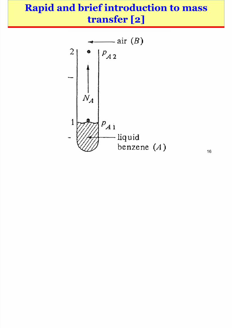
16
Rapid and brief introduction to masstransfer [2]
8/9/2019 SLides -1 TP
http://slidepdf.com/reader/full/slides-1-tp 17/112
17
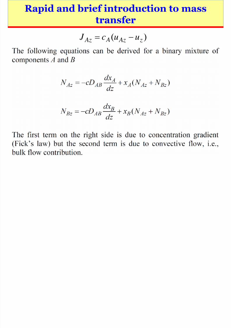
Rapid and brief introduction to masstransfer
)( z Az A Az uuc J −=
8/9/2019 SLides -1 TP
http://slidepdf.com/reader/full/slides-1-tp 18/112
18
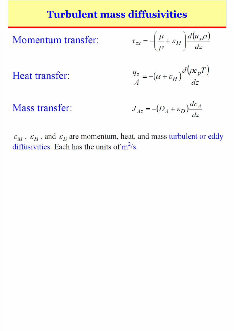
Turbulent mass diffusivities
8/9/2019 SLides -1 TP
http://slidepdf.com/reader/full/slides-1-tp 19/112
19
Turbulent mass diffusivities
8/9/2019 SLides -1 TP
http://slidepdf.com/reader/full/slides-1-tp 20/112
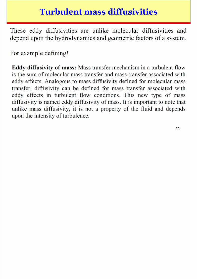
20
Turbulent mass diffusivities
8/9/2019 SLides -1 TP
http://slidepdf.com/reader/full/slides-1-tp 21/112

8/9/2019 SLides -1 TP
http://slidepdf.com/reader/full/slides-1-tp 22/112
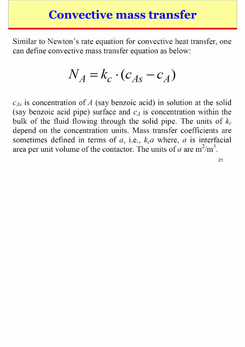
22
Convective mass transfer

8/9/2019 SLides -1 TP
http://slidepdf.com/reader/full/slides-1-tp 23/112
23
Convective mass transfer
8/9/2019 SLides -1 TP
http://slidepdf.com/reader/full/slides-1-tp 24/112
24
Convective mass transfer
C ti t f

8/9/2019 SLides -1 TP
http://slidepdf.com/reader/full/slides-1-tp 25/112
25
Convective mass transfercorrelations
8/9/2019 SLides -1 TP
http://slidepdf.com/reader/full/slides-1-tp 26/112
26
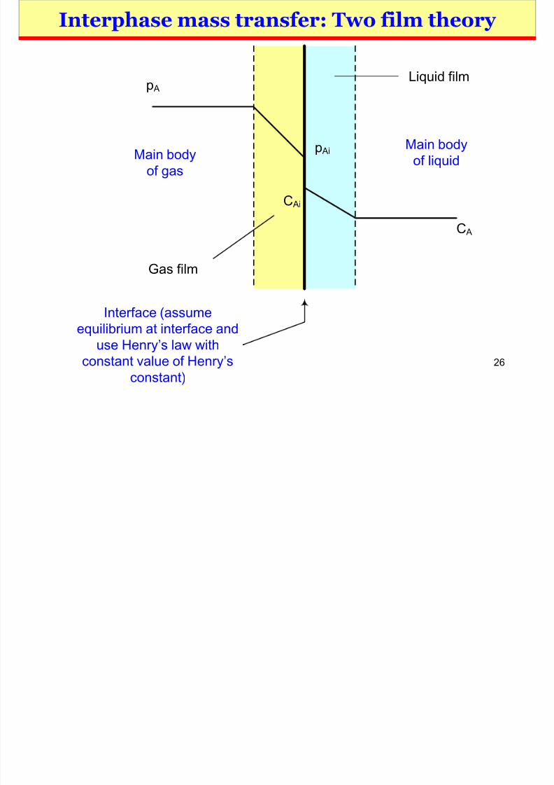
Interphase mass transfer: Two film theory
p A
p Ai
C Ai
C A
Main body
of gas
Main body
of liquid
Liquid film
Gas film
C Ai
p Ai
Interface (assume
equilibrium at interface and
use Henry’s law with
constant value of Henry’sconstant)

8/9/2019 SLides -1 TP
http://slidepdf.com/reader/full/slides-1-tp 27/112
27
Two-film theory: Overall masstransfer coefficient
Diff i ffi i t

8/9/2019 SLides -1 TP
http://slidepdf.com/reader/full/slides-1-tp 28/112
28
Diffusion coefficient ormass diffusivity
The proportionality coefficient for the Fick’s law formolecular transfer is mass diffusivity or diffusioncoefficient.
Like viscosity and thermal conductivity, diffusion
coefficient is also measured under molecular transportconditions and not in the presence of eddies (turbulentflow).
The SI units of mass diffusivity are m2/s.
1 m2/s = 3.875×104 ft2/h1 cm2/s = 10 ‒4 m2/s = 3.875 ft2/h
1 m2/h = 10.764 ft2/h
1 centistokes = 10 ‒2 cm2/s
Diff i ffi i t
8/9/2019 SLides -1 TP
http://slidepdf.com/reader/full/slides-1-tp 29/112
29
Diffusion coefficient ormass diffusivity
Why do we use a small diameter capillary for themeasurement of viscosity of a liquid?
Bring to mind Ostwald’s viscometer.
8/9/2019 SLides -1 TP
http://slidepdf.com/reader/full/slides-1-tp 30/112
30
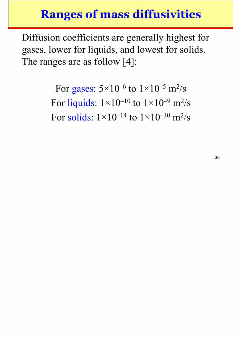
Ranges of mass diffusivities
Diffusion coefficients are generally highest forgases, lower for liquids, and lowest for solids.The ranges are as follow [4]:
For gases: 5×10 ‒6 to 1×10 ‒5 m2/s
For liquids: 1×10 ‒10 to 1×10 ‒9 m2/s
For solids: 1×10 ‒14
to 1×10 ‒10
m2
/s
Diffusion coefficient or

8/9/2019 SLides -1 TP
http://slidepdf.com/reader/full/slides-1-tp 31/112
31
Diffusion coefficient ormass diffusivity
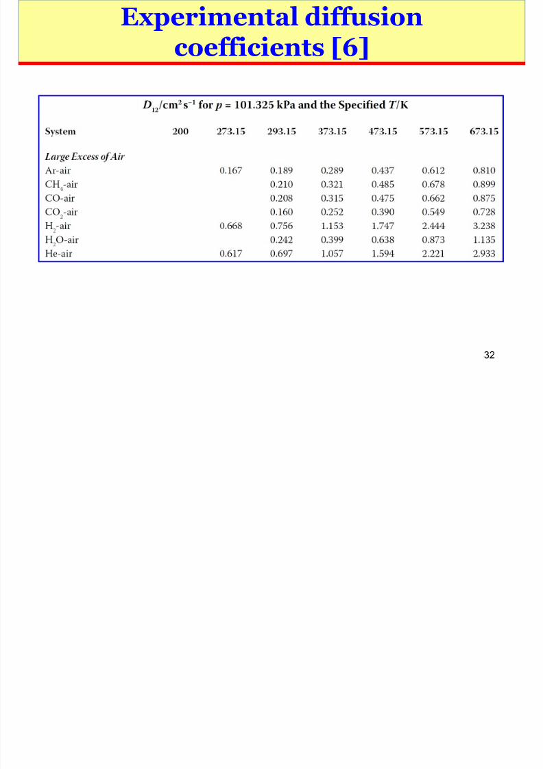
Diffusion coefficients may be obtained by doingexperiments in the laboratory.
Diffusion coefficients may be obtained fromexperimentally measured values by various
researchers in the field. Many of these data iscollected in handbooks, etc.
When experimental values are not found, diffusioncoefficients may be estimated using theoretical,semi-empirical (semi-theoretical), or empiricalcorrelations.
Experimental diffusion
8/9/2019 SLides -1 TP
http://slidepdf.com/reader/full/slides-1-tp 32/112
32
Experimental diffusioncoefficients [6]
Experimental diffusion

8/9/2019 SLides -1 TP
http://slidepdf.com/reader/full/slides-1-tp 33/112
33
Experimental diffusioncoefficients: References
Lide, D.R. 2007. CRC Handbook of chemistry and physics. 87th ed. CRC Press.
Poling, B.E.; Prausnitz, J.H.; O’Connell, J.P. 2000.The properties of gases and liquids. 5th ed. McGraw-
Hill.Green. D.W.; Perry, R.H. 2008. Perry’s chemicalengineers’ handbook. 8th ed. McGraw-Hill.
Please populate the list.

8/9/2019 SLides -1 TP
http://slidepdf.com/reader/full/slides-1-tp 34/112
Diffusion coefficient for gases at
8/9/2019 SLides -1 TP
http://slidepdf.com/reader/full/slides-1-tp 35/112
35
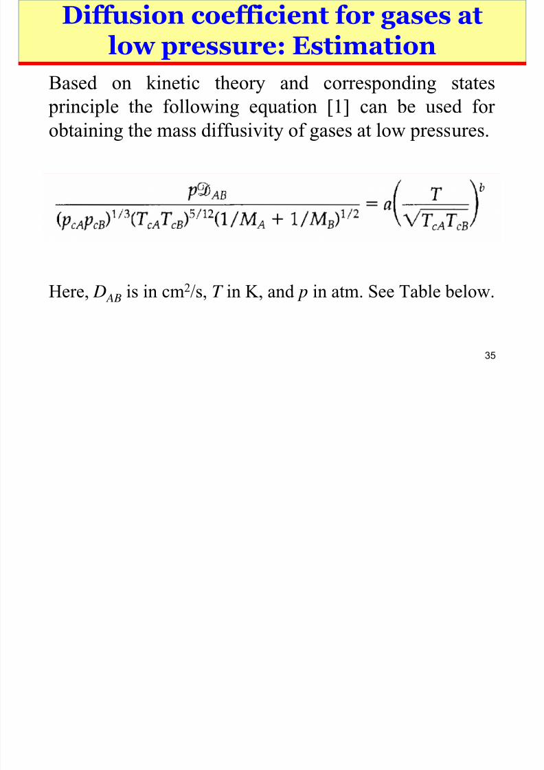
Diffusion coefficient for gases atlow pressure: Estimation
Based on kinetic theory and corresponding states principle the following equation [1] can be used forobtaining the mass diffusivity of gases at low pressures.
Here, D AB is in cm2/s, T in K, and p in atm. See Table below.
Diffusion coefficient for gases at

8/9/2019 SLides -1 TP
http://slidepdf.com/reader/full/slides-1-tp 36/112
36
The equation fits the experimental data well at atmospheric
pressure within an average error of 6 ‒ 8%.
Situation a b
For non-polar gas pairs (excluding He and H2)
2.745×10 ‒4 1.823
H2O and a nonpolar gas 3.640×10 ‒4 2.334
Diffusion coefficient for gases atlow pressure: Estimation

8/9/2019 SLides -1 TP
http://slidepdf.com/reader/full/slides-1-tp 37/112

8/9/2019 SLides -1 TP
http://slidepdf.com/reader/full/slides-1-tp 38/112
38
Homework problem
Estimate D AB for the systems CO2-N2O, CO2-N2, CO2-O2 , N2-O2, and H2-N2 at 273.2 and 1 atm and comparethe results with the experimental values given in Table
17.1-1 [1]. Also for H2O-N2 at 308 K and 1 atm andcompare similarly.
Diffusion coefficient for gases at
8/9/2019 SLides -1 TP
http://slidepdf.com/reader/full/slides-1-tp 39/112
39
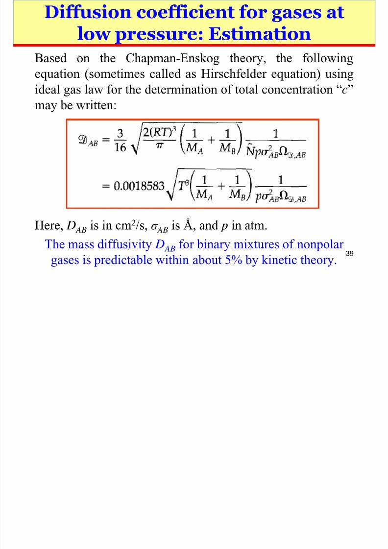
Diffusion coefficient for gases atlow pressure: Estimation
Based on the Chapman-Enskog theory, the followingequation (sometimes called as Hirschfelder equation) usingideal gas law for the determination of total concentration “c”may be written:
Here, D AB is in cm2/s, σ AB is Å, and p in atm.
The mass diffusivity D AB for binary mixtures of nonpolar
gases is predictable within about 5% by kinetic theory.
Diffusion coefficient for gases at

8/9/2019 SLides -1 TP
http://slidepdf.com/reader/full/slides-1-tp 40/112
40
Diffusion coefficient for gases atlow pressure: Estimation
The parameters σ AB and ε AB could, in principle, be determineddirectly from accurate measurement of D AB over a wide range oftemperatures. Suitable data are not yet available for many gas pairs, one may have to resort to using some other measurable property, such as the viscosity of a binary mixture of A and B. In
the event that there are no such data, then we can estimate themfrom the following combining rules for non-polar gas pairs.
Use of these combining rules enables us to predict values of D AB within about 6% by use of viscosity data on the pure species A and B, or within about 10% if the Lennard-Jones parameters for A and B are estimated from boiling point data as discussed in
Chapter 1 of the text [1].
Diffusion coefficient for gases at

8/9/2019 SLides -1 TP
http://slidepdf.com/reader/full/slides-1-tp 41/112
41
Diffusion coefficient for gases atlow pressure: Estimation
The Lennard-Jones parameters can be obtained from theAppendix of the text book [1] and in cases when not known can be estimated as below:
The boiling conditions are normal conditions, i.e., at 1 atm.

8/9/2019 SLides -1 TP
http://slidepdf.com/reader/full/slides-1-tp 42/112
42
Lennard-Jones potential [7]
Diffusion coefficient for gases at

8/9/2019 SLides -1 TP
http://slidepdf.com/reader/full/slides-1-tp 43/112
43
Diffusion coefficient for gases atlow pressure: Estimation
The collision integral can be obtained using dimensionlesstemperature from the Appendix of the text book [1]. Toavoid interpolation, a graphical relationship for collision integralis given in the next slide.
A mathematical relationship by Neufeld is recommended for
computational (spreadsheet) work [5].
Diffusion coefficient for gases at low

8/9/2019 SLides -1 TP
http://slidepdf.com/reader/full/slides-1-tp 44/112
44
Diffusion coefficient for gases at lowpressure: Estimation [4]
Diffusion coefficient for gases at

8/9/2019 SLides -1 TP
http://slidepdf.com/reader/full/slides-1-tp 45/112
45
Diffusion coefficient for gases atlow pressure: Estimation
The effect of composition (concentration) is notaccommodated in the above equation. The effect ofconcentration in real gases is usually negligible andeasily ignored, especially at low pressures. For high
pressure gases, some effects, though small, areobserved.
Diffusion coefficient for gases at
8/9/2019 SLides -1 TP
http://slidepdf.com/reader/full/slides-1-tp 46/112
46
Diffusion coefficient for gases atlow pressure: Estimation
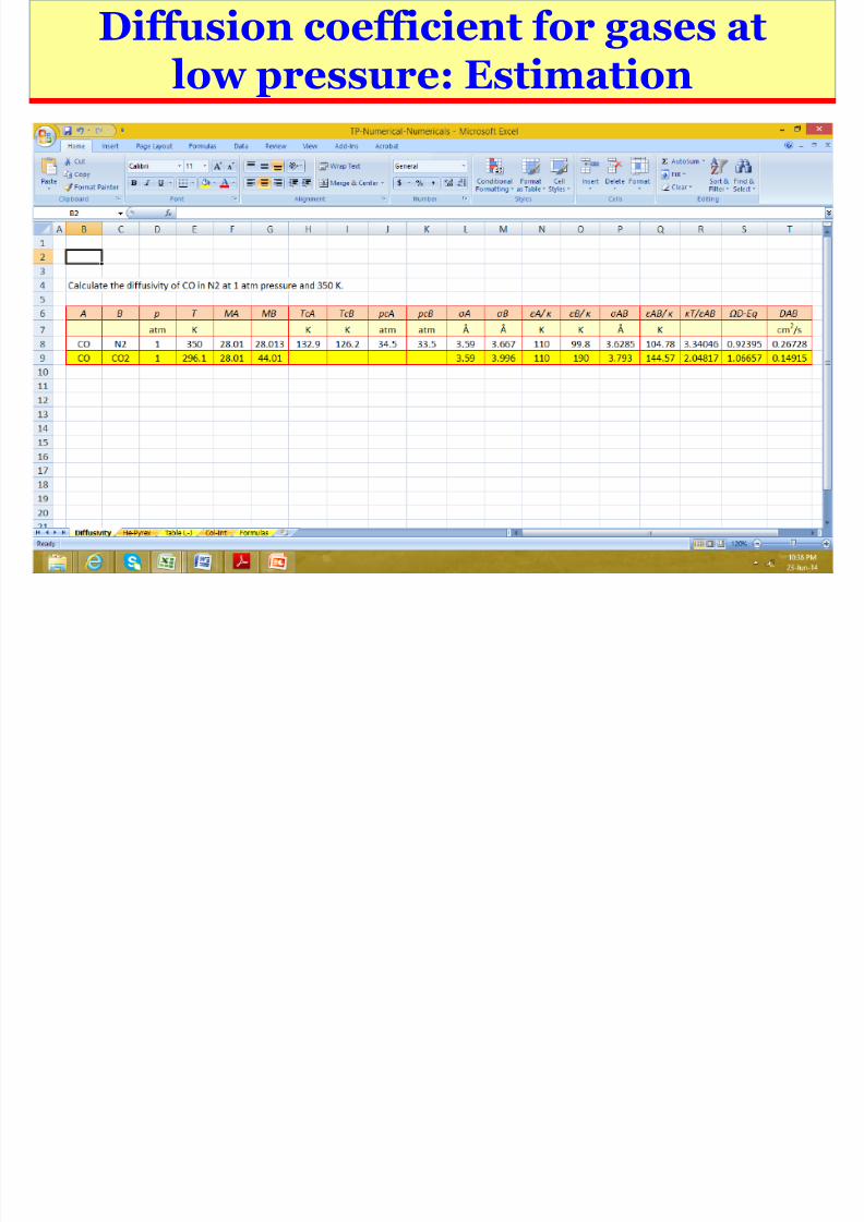
Example 17.3-1 [1]:
Predict the value of D AB for the system CO-CO2 at296.1 K and 1 atm total pressure.
Use the equation based on Chapman-Enskog theory as
discussed above. The values of Lennard-Jones Potentialand others may be found in Appendix E of the text [1].
Diffusion coefficient for gases at
8/9/2019 SLides -1 TP
http://slidepdf.com/reader/full/slides-1-tp 47/112
47
Diffusion coefficient for gases atlow pressure: Estimation
Diffusion coefficient for gases at

8/9/2019 SLides -1 TP
http://slidepdf.com/reader/full/slides-1-tp 48/112
48
Diffusion coefficient for gases atlow pressure: Estimation
The above equation (Hirschfelder equation) is used toextrapolate the experimental data. Using the aboveequation, the diffusion coefficient can be predicted atany temperature and any pressure below 25 atm [4]
using the following equation.
2
F ll ’ ti
8/9/2019 SLides -1 TP
http://slidepdf.com/reader/full/slides-1-tp 49/112
49
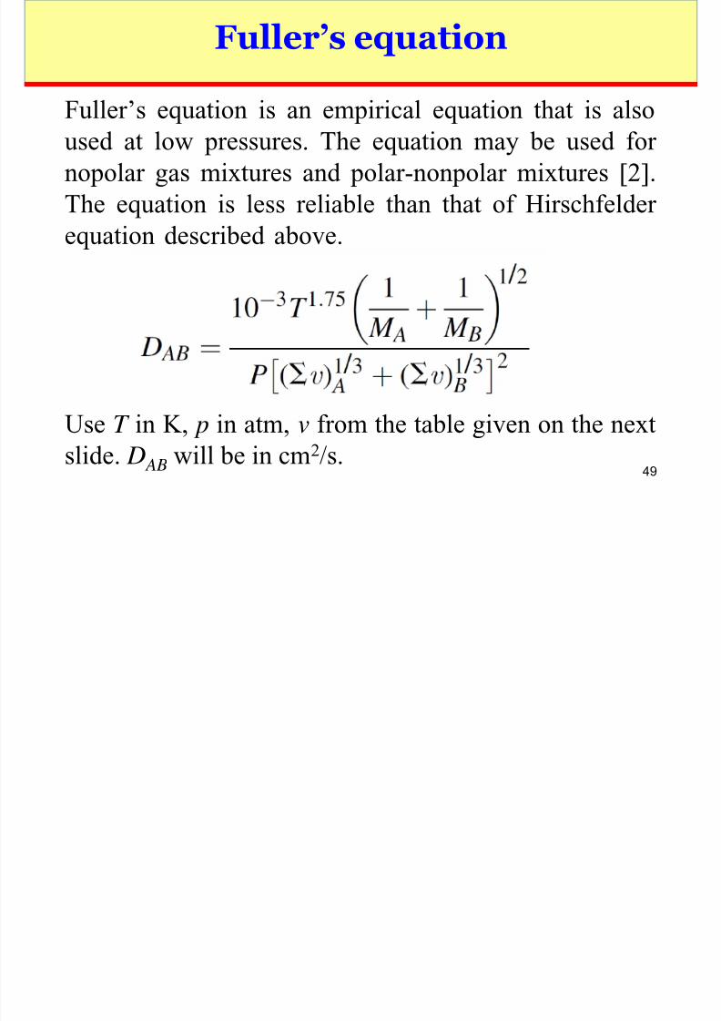
Fuller’s equation
Fuller’s equation is an empirical equation that is alsoused at low pressures. The equation may be used fornopolar gas mixtures and polar-nonpolar mixtures [2].The equation is less reliable than that of Hirschfelder
equation described above.
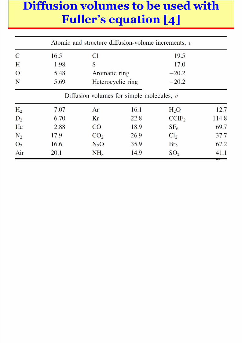
Use T in K, p in atm, v from the table given on the nextslide. D AB will be in cm2/s.
Diffusion volumes to be used with
8/9/2019 SLides -1 TP
http://slidepdf.com/reader/full/slides-1-tp 50/112
50
Diffusion volumes to be used withFuller’s equation [4]
f ll ’ i
8/9/2019 SLides -1 TP
http://slidepdf.com/reader/full/slides-1-tp 51/112
51
Use of Fuller’s equation
Example problem [2]:
Normal butanol ( A) is diffusing through air ( B) at 1 atmabs. Using the Fuller’s equation, estimate the diffusivity D AB for the following temperatures.
a) For 0 °C b) 25.9 °C
c) 0 °C and 2.0 atm abs.
Diffusion coefficient for gases at
8/9/2019 SLides -1 TP
http://slidepdf.com/reader/full/slides-1-tp 52/112
52
Diffusion coefficient for gases athigh density
The behavior of gases at high pressures (densegases) and of liquids is not well understood anddifficult to interpret to a mathematicalevaluation. The following approaches can beused for estimating the mass diffusivity of gasesat high pressures.
Diffusion coefficient for gases at high
8/9/2019 SLides -1 TP
http://slidepdf.com/reader/full/slides-1-tp 53/112
53
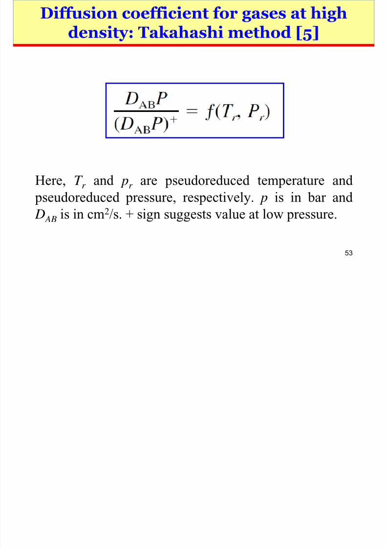
Diffusion coefficient for gases at highdensity: Takahashi method [5]
Here, T r and pr are pseudoreduced temperature and
pseudoreduced pressure, respectively. p is in bar and D AB is in cm2/s. + sign suggests value at low pressure.
Diffusion coefficient for gases at high

8/9/2019 SLides -1 TP
http://slidepdf.com/reader/full/slides-1-tp 54/112
54
Diffusion coefficient for gases at highdensity: Takahashi method [5]
Tr
Diffusion coefficient for gas mixtures [1]

8/9/2019 SLides -1 TP
http://slidepdf.com/reader/full/slides-1-tp 55/112
55
g [ ]
Diffusion coefficient for gas

8/9/2019 SLides -1 TP
http://slidepdf.com/reader/full/slides-1-tp 56/112
56
us o coe c e t o gasmixtures [1]
The value of can be obtained from the graph above by knowing reduced temperature and reduced pressure.
Where, D AB is in cm2/s, T in K, and pc in atm.
Diffusion coefficient for gas

8/9/2019 SLides -1 TP
http://slidepdf.com/reader/full/slides-1-tp 57/112
57
gmixtures
The above method is quite good for gases at low pressures. At high pressures, due to the lack of largenumber of experimental data, a comparison is difficultto make. The method is therefore suggested only for
gases at low pressures.
The value of cD AB rather than D AB is becausecD AB is usually found in mass transferexpressions and the dependence of pressure and
temperature is simpler [1].
Diffusion coefficient for gas

8/9/2019 SLides -1 TP
http://slidepdf.com/reader/full/slides-1-tp 58/112
58
gmixtures at high density
Example 17.2-3 [1]:
Estimate cD AB for a mixture of 80 mol% CH4 and 20mol% C2H6 at 136 atm and 313 K. It is known that, at 1atm and 293 K, the molar density is c = 4.17 × 10 ‒ 5
gmol/cm3 and D AB 0.163 cm2/s.
P bl A [ ]
8/9/2019 SLides -1 TP
http://slidepdf.com/reader/full/slides-1-tp 59/112
59
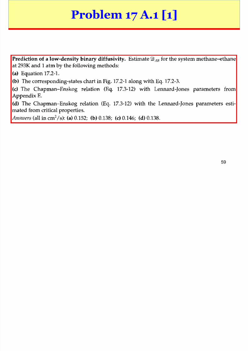
Problem 17 A.1 [1]
Diffusion coefficient for liquid
8/9/2019 SLides -1 TP
http://slidepdf.com/reader/full/slides-1-tp 60/112
60
qmixtures
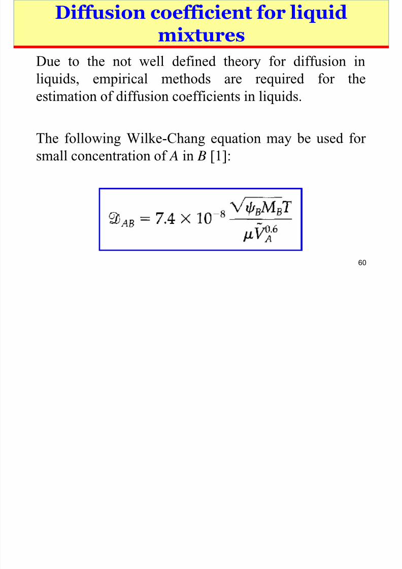
Due to the not well defined theory for diffusion inliquids, empirical methods are required for theestimation of diffusion coefficients in liquids.
The following Wilke-Chang equation may be used forsmall concentration of A in B [1]:
Diffusion coefficient for liquid

8/9/2019 SLides -1 TP
http://slidepdf.com/reader/full/slides-1-tp 61/112
61
qmixtures
In the above equation, Ṽ is molar volume of solute A in cm3/mol as liquid at its boiling point, μ is viscosity ofsolution in cP, ψ B is an association parameter for thesolvent, and T is absolute temperature in K.
Recommended values of ψ B are: 2.6 for water; 1.9 formethanol; 1.5 for ethanol; 1.0 for benzene, ether,heptane, and other unassociated solvents.
The equation is good for dilute solutions of
nondissociating solutes. For such solutions, it is usuallygood within ±10%.
Selected molar volumes at normal

8/9/2019 SLides -1 TP
http://slidepdf.com/reader/full/slides-1-tp 62/112
62
boiling points [4]
Atomic volumes for calculating molar volumes andcorrections [4]

8/9/2019 SLides -1 TP
http://slidepdf.com/reader/full/slides-1-tp 63/112
63
corrections [4]
Diffusion coefficient for liquid
8/9/2019 SLides -1 TP
http://slidepdf.com/reader/full/slides-1-tp 64/112
64
qmixtures
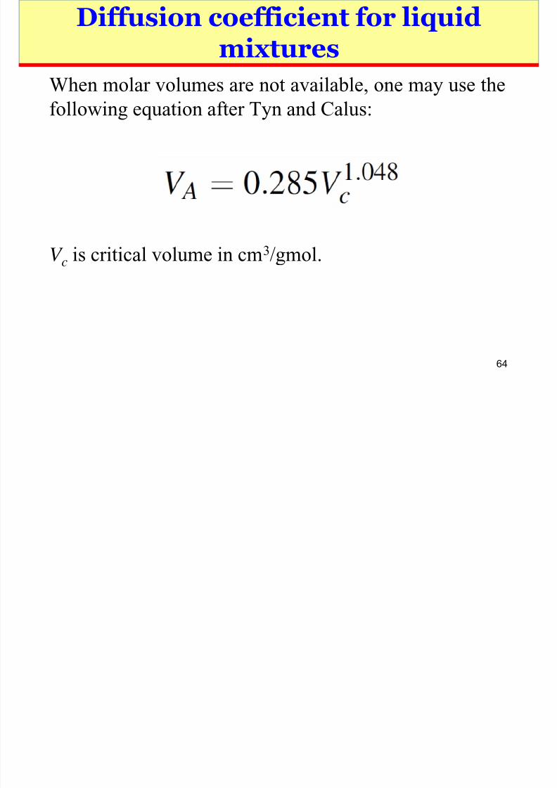
When molar volumes are not available, one may use thefollowing equation after Tyn and Calus:
V c is critical volume in cm3/gmol.
Diffusion coefficient for liquid

8/9/2019 SLides -1 TP
http://slidepdf.com/reader/full/slides-1-tp 65/112
65
qmixtures
Example 17.4-1 [1]:
Estimate D AB for a dilute solution of TNT (2,4,6-trinitrotoluene) in benzene at 15 °C. Take TNT as A andtoluene as B component. Molar volume of TNT is 140
cm3/mol. Hint : As dilute solution, use viscosity of benzeneinstead of solution.
Example 5 [4, 418]:
Estimate the diffusion coefficient of ethanol in a dilutesolution of water at 10 °C.
Homework problem

8/9/2019 SLides -1 TP
http://slidepdf.com/reader/full/slides-1-tp 66/112
66
Homework problem
Example 6.3-2 [2]:
Predict the diffusion coefficient of acetone(CH3COCH3) in water at 25 °C and 50 °C using theWilke-Chang equation. The experimental value is 1.28
× 10 ‒
9 m2/s at 25 °C.
Further reading

8/9/2019 SLides -1 TP
http://slidepdf.com/reader/full/slides-1-tp 67/112
67
g
Poling, B.E.; Prausnitz,
J.H.; O’Connell, J.P.2000. The properties ofgases and liquids. 5th ed.
McGraw-Hill.
Excellent reference for
the estimation of massdiffusivities. See Chapter11 of the book.
Homework problems

8/9/2019 SLides -1 TP
http://slidepdf.com/reader/full/slides-1-tp 68/112
68
Homework problems
Questions for discussions [1, pp. 538–539]:
1, 3, 4, and 7.
Problems [1, pp. 539–541]:
17A.4, 17A.5, 17A.6, 17A.9, and 17A.10.
Shell mass balance

8/9/2019 SLides -1 TP
http://slidepdf.com/reader/full/slides-1-tp 69/112
69
Shell mass balance
Why do we need shell (smallcontrol element ) mass balance?
Shell mass balance
8/9/2019 SLides -1 TP
http://slidepdf.com/reader/full/slides-1-tp 70/112
70
Shell mass balance
We need, because, we desire to know what is happeninginside. In other words, we want to know the differentialor point to point molar flux and concentration
distributions with in a system, i.e., we will represent thesystem in terms of differential equations. Macro or bulk balances such as that applied in material balancecalculations only give input and output information and
do not tell what happens inside the system.
Steps involved in shell mass

8/9/2019 SLides -1 TP
http://slidepdf.com/reader/full/slides-1-tp 71/112
71
balance
o Select a suitable coordinate system (rectangular,cylindrical, or spherical) to represent the given problem.
o Accordingly, select a suitable small control elementor shell of finite dimensions in the given system.
o Define the appropriate assumptions and apply mass balance over the shell geometry.
o Let the shell dimensions approach zero (differentialdimensions) and using the definition of derivation,obtain the first order differential equation. The solutionof this equation gives the molar flux distribution.
Steps involved in shell mass

8/9/2019 SLides -1 TP
http://slidepdf.com/reader/full/slides-1-tp 72/112
72
balance
o Insert the definition of molar flux in the abovedifferential equation, a second order differentialequation will be the result.
o Define the appropriate boundary conditions and solve
the second order differential equation to obtain theconcentration profile and the values of the average flux.
Coordinate systems [8]

8/9/2019 SLides -1 TP
http://slidepdf.com/reader/full/slides-1-tp 73/112
73
Coordinate systems [8]
See Appendix A.6 of the text [1].
General mass balance equation
8/9/2019 SLides -1 TP
http://slidepdf.com/reader/full/slides-1-tp 74/112
74
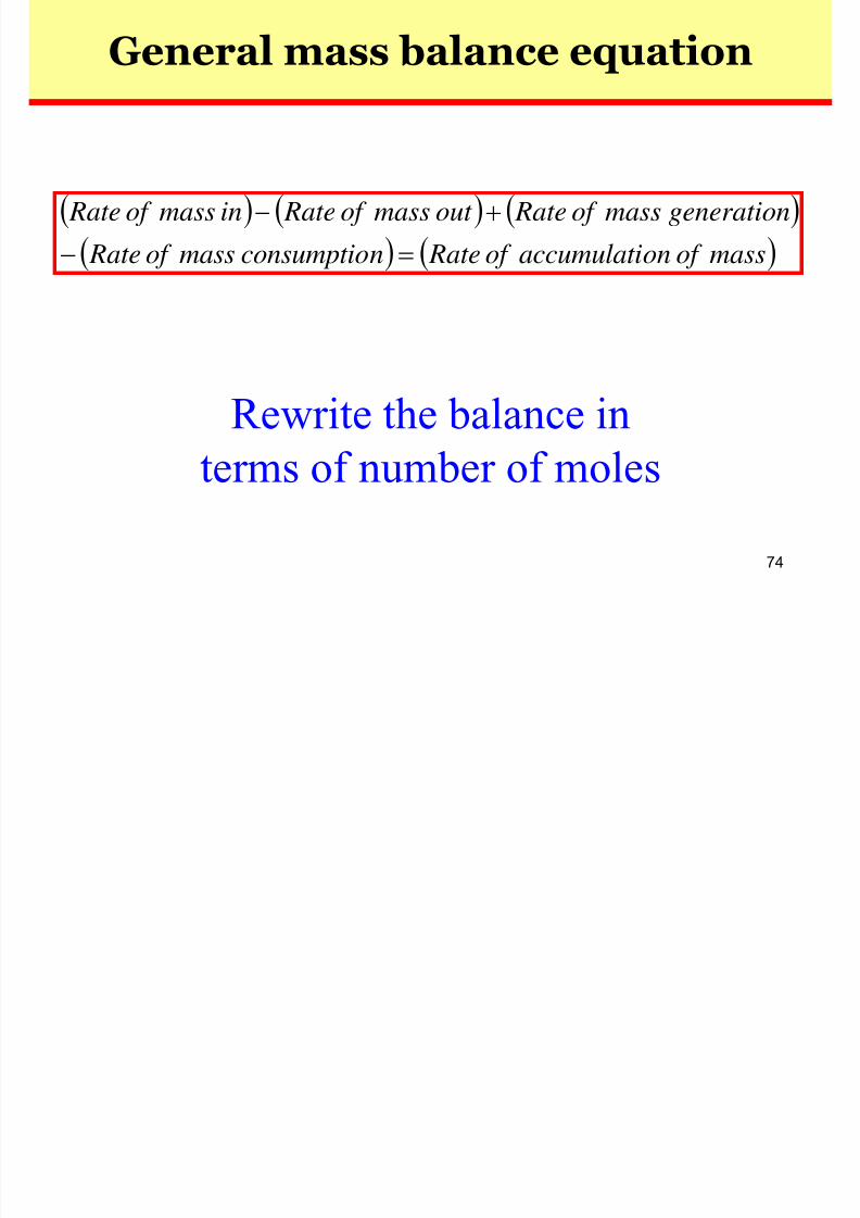
General mass balance equation
Rewrite the balance interms of number of moles
( ) ( ) ( )( ) ( )massof onaccumulatiof Ratenconsumptiomassof Rate
generationmassof Rateout massof Rateinmassof Rate
=−
+−
Modeling problem

8/9/2019 SLides -1 TP
http://slidepdf.com/reader/full/slides-1-tp 75/112
75
Modeling problem
Diffusion through a stagnant gas film
Diffusion through a stagnant gas

8/9/2019 SLides -1 TP
http://slidepdf.com/reader/full/slides-1-tp 76/112
76
film [1]
Concentration
distribution
Shell
Diffusion through a stagnant gas
8/9/2019 SLides -1 TP
http://slidepdf.com/reader/full/slides-1-tp 77/112
77
film
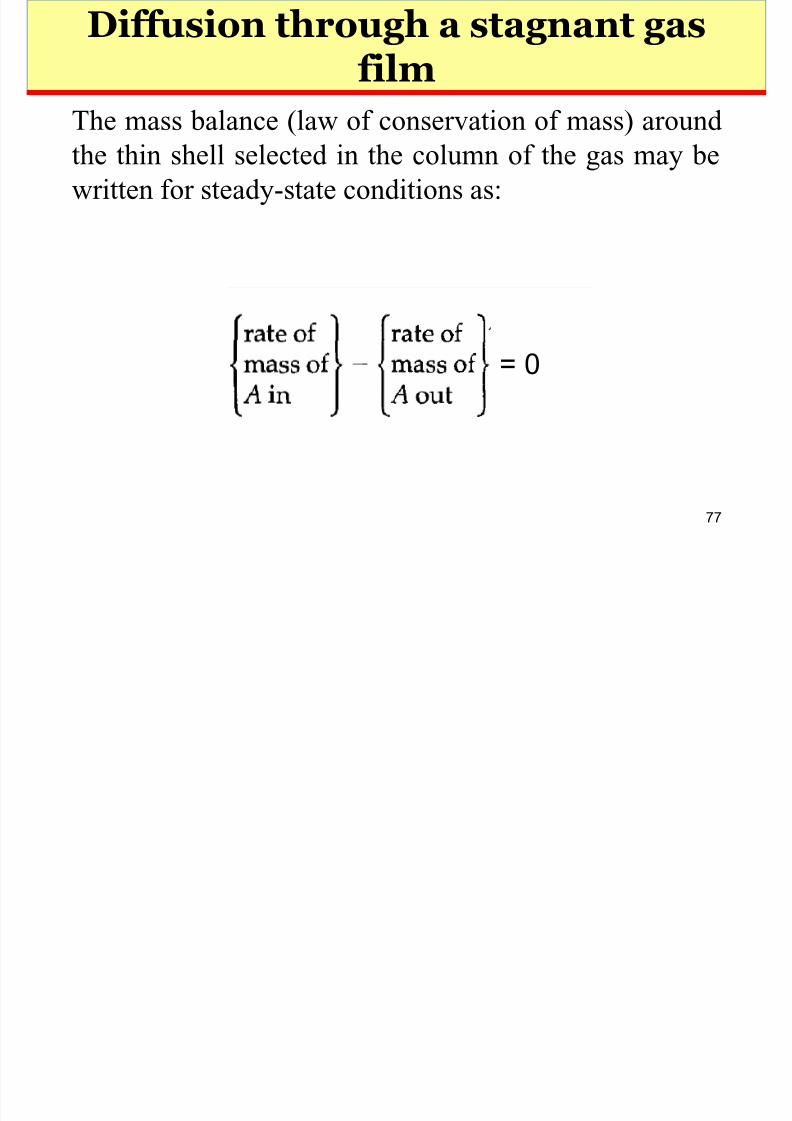
The mass balance (law of conservation of mass) aroundthe thin shell selected in the column of the gas may bewritten for steady-state conditions as:
= 0
Diffusion through a stagnant gas

8/9/2019 SLides -1 TP
http://slidepdf.com/reader/full/slides-1-tp 78/112
78
film
As no reaction is occurring so the third term on the previous slide is not needed. The mass balance then can be written as
Units of are
Where, S is the cross-sectional area of the column and N AZ is molar flux of A in z direction.
0=⋅−⋅
∆+ z z Az z Az N S N S
s
mol
sm
molm
2
2 =
⋅⋅
Az N S ⋅
Diffusion through a stagnant gas

8/9/2019 SLides -1 TP
http://slidepdf.com/reader/full/slides-1-tp 79/112
79
film
Dividing throughput by and taking , it may be shown that
We know for combined molecular and convective flux
As gas B is stagnant (non-diffusing), so and theabove equation becomes
0=−dz
dN Az
z∆ 0→∆ z
)( Bz Az A A
AB Az N N xdz
dxcD N ++−=
0= Bz N
Az A A
AB Az N x
dz
dxcD N +−=
Diffusion through a stagnant gasfil

8/9/2019 SLides -1 TP
http://slidepdf.com/reader/full/slides-1-tp 80/112
80
film
dz
dx
x
cD N A
A
AB Az
−=1
01
=
− dz
dx
x
cD
dz
d A
A
AB
Diffusion through a stagnant gasfil i fil
8/9/2019 SLides -1 TP
http://slidepdf.com/reader/full/slides-1-tp 81/112
81
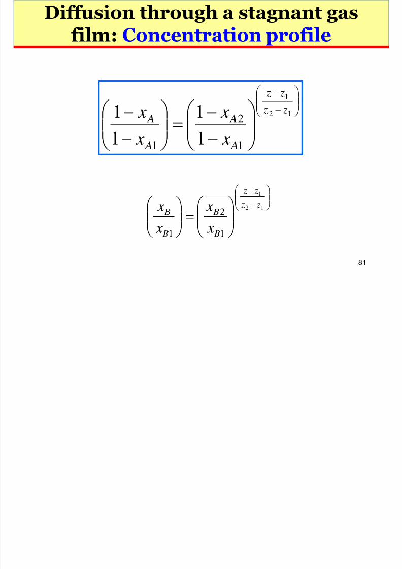
film: Concentration profile
−
−
−
−=
−
− 12
1
1
2
1 1
1
1
1 z z
z z
A
A
A
A
x
x
x
x
−
−
=
12
1
1
2
1
z z
z z
B
B
B
B
x
x
x
x
Diffusion through a stagnant gasfil l fl

8/9/2019 SLides -1 TP
http://slidepdf.com/reader/full/slides-1-tp 82/112
82
film: Molar flux
dzdx
xcD N A
A
AB Az
−−=
1
−−
−=
1
2
12 11ln
)( A
A AB Az
x x
z zcD N
−=
1
2
12
ln)( B
B AB Az
x
x
z z
cD N
Diffusion through a stagnant gasfil

8/9/2019 SLides -1 TP
http://slidepdf.com/reader/full/slides-1-tp 83/112
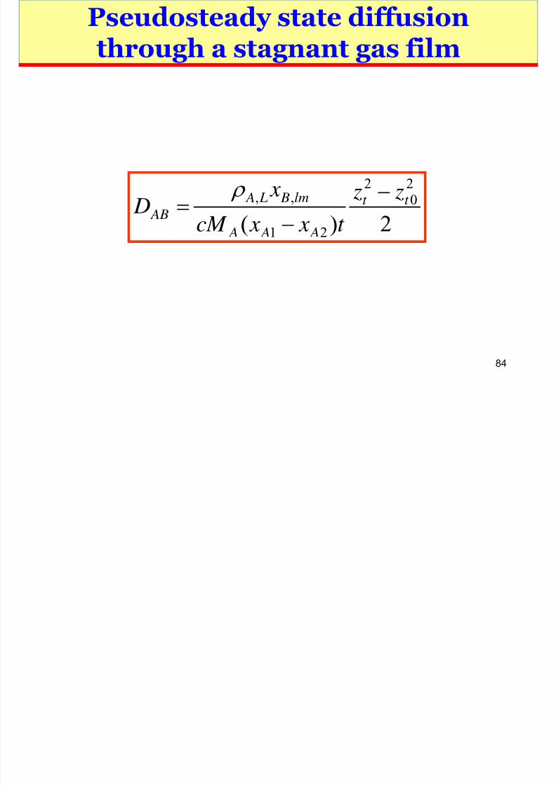
83
film
lm B
A A AB Az x
x x
z z
cD N
,21
12 )(
−
−=
lm B
A A AB Az
p
p p
z z RT
p D N
,
21
12 )(
−
−=
Using ideal gas law
−
−
−=
1
2
21,
1
1ln
A
A
A Alm B
x
x
x x x
−=
1
2
12,
ln
B
B
B Blm B
x
x
x x x
or
Where
8/9/2019 SLides -1 TP
http://slidepdf.com/reader/full/slides-1-tp 84/112
Diffusion through a stagnant gasfil A li i

8/9/2019 SLides -1 TP
http://slidepdf.com/reader/full/slides-1-tp 85/112
85
film: Applications
The results are useful in:
o
measuring the mass diffusion coefficiento studying film models for mass transfer.
Diffusion through a stagnant gasfil D f t
8/9/2019 SLides -1 TP
http://slidepdf.com/reader/full/slides-1-tp 86/112
86
film: DefectsIn the present model, “it is assumed that there is a sharp transition
from a stagnant film to a well-mixed fluid in which theconcentration gradients are negligible. Although this model is
physically unrealistic, it has nevertheless proven useful as asimplified picture for correlating mass transfer coefficients” [1]
The present method for measuring gas-phase diffusivitiesinvolves several defects:
“the cooling of the liquid by evaporation
the concentration of nonvolatile impurities at the interfacethe climbing of the liquid up the walls of the tube and
curvature of the meniscus” [1]
Problem [10]

8/9/2019 SLides -1 TP
http://slidepdf.com/reader/full/slides-1-tp 87/112
87
Problem [10]
The water surface in an open cylindrical tank is 25 ft below the
top. Dry air is blown over the top of the tank and the entiresystem is maintained at 65 °F and 1 atm. If the air in the tank isstagnant, determine the diffusion rate of the water. Use diffusivityas 0.97 ft2/h at 65f water in air °F and 1 atm.
[Universal gas constant = 0.73 ft3-atm/lbmol-°R]
Problem [10]

8/9/2019 SLides -1 TP
http://slidepdf.com/reader/full/slides-1-tp 88/112
88
ob e [ 0]
At the bottom of a cylindrical container is n-butanol. Pure air is
passed over the open top of the container. The pressure is 1 atmand the temperature is 70 °F. The diffusivity of air-n-butanol is8.57×10 ‒ 6 m2/s at the given conditions. If the surface of n-butanolis 6.0 ft below the top f the container, calculate the diffusion rate
of n-butanol. Vapor pressure of n-butanol is 0.009 atm at thegiven conditions.
[Universal gas constant = 0.08205 m3-atm/kmol-K]
Homework problems

8/9/2019 SLides -1 TP
http://slidepdf.com/reader/full/slides-1-tp 89/112
89
p
Example 18.2-2 [1]Problem 18A.1 and 18A.6 [1]
Diffusion of A through stagnant gas filmin sphe ical coo dinates
8/9/2019 SLides -1 TP
http://slidepdf.com/reader/full/slides-1-tp 90/112
90
in spherical coordinates
A spherical particle A having radius r 1 issuspended in a gas B. The component A diffusesthrough the gas film having radius r 2. If the gas
B is stagnant, i.e., not diffusing into A, derive an
expression for molar flux of A into B.
Diffusion of A through stagnant gas filmin spherical coordinates

8/9/2019 SLides -1 TP
http://slidepdf.com/reader/full/slides-1-tp 91/112
91
in spherical coordinates
Diffusion of A through stagnant gas filmin spherical coordinates: Pls check

8/9/2019 SLides -1 TP
http://slidepdf.com/reader/full/slides-1-tp 92/112
92
in spherical coordinates: Pls check
−=
1
2
1
2
121 ln)( B
B AB
Ar x
x
r
r
r r
cD
N
−
−
−=
1
2
1
2
12
11
1ln
)( A
A AB Ar
x
x
r
r
r r
cD N
Diffusion of A through stagnant gas filmin spherical coordinates

8/9/2019 SLides -1 TP
http://slidepdf.com/reader/full/slides-1-tp 93/112
93
in spherical coordinates
Derive concentration profile as shown below for the system just
discussed in the previous slides.
)/1()/1(
)/1()/1(
1
2
1
21
1
1
1
1
1 r r
r r
A
A
A
A
x
x
x
x −
−
−
−=
−
−
Diffusion of A through stagnant gas filmin cylindrical coordinates
8/9/2019 SLides -1 TP
http://slidepdf.com/reader/full/slides-1-tp 94/112
94
in cylindrical coordinates
A cylindrical particle of benzoic acid A havingradius r 1 is suspended in a gas B. The component A diffuses through the gas film having radius r 2.If the gas B is stagnant, i.e., not diffusing into A,
derive an expression for molar flux of A into B.Also work out the concentration profile for thesituation.
Diffusion of A through Pyrex glass tube

8/9/2019 SLides -1 TP
http://slidepdf.com/reader/full/slides-1-tp 95/112
95
g y g
Diffusion of A through Pyrex glass tube

8/9/2019 SLides -1 TP
http://slidepdf.com/reader/full/slides-1-tp 96/112
96
)/ln(
)(
121
211
R R R
cc D N A A AB
AR
−=
)/ln(
)/ln(
12
2
21
2
R R
r R
cc
cc
A A
A A =−
−
)/ln()(
121
211
R R R x xcD N A A AB
AR −=
Separation of helium from gas mixture[4]

8/9/2019 SLides -1 TP
http://slidepdf.com/reader/full/slides-1-tp 97/112
97
Homework problems

8/9/2019 SLides -1 TP
http://slidepdf.com/reader/full/slides-1-tp 98/112
98
Problem 18B.7 [1]Problem 18B.9 [1]

8/9/2019 SLides -1 TP
http://slidepdf.com/reader/full/slides-1-tp 99/112
Diffusion with a heterogeneouschemical reaction [1]

8/9/2019 SLides -1 TP
http://slidepdf.com/reader/full/slides-1-tp 100/112
100
chemical reaction [1]
Diffusion with a heterogeneouschemical reaction

8/9/2019 SLides -1 TP
http://slidepdf.com/reader/full/slides-1-tp 101/112
101
chemical reaction
−
=
02
1
1
1ln
2
A
AB AZ
x
cD N
δ
)/(1
02
112
11δ z
A A x x
−
−=
−
Diffusion with a heterogeneouschemical reaction [2]

8/9/2019 SLides -1 TP
http://slidepdf.com/reader/full/slides-1-tp 102/112
102
chemical reaction [2]
Pure gas A diffuses from point 1 at a partial pressure of 101.32
kPa to point 2 a distance 2.0 mm away. At point 2 it undergoes achemical reaction at the catalyst surface and .Component B diffuses back at steady-state. The total pressure is p = 101.32 kPa. The temperature is 300 K and D AB = 0.15×10 ‒4
m2
/s.a) For instantaneous rate of reaction, calculate x A2 and N A.
b) For a slow reaction where k = 5.63×10 ‒ 3 m/s, calculate x A2 and N A.
B A 2→
Diffusion with a heterogeneouschemical reaction

8/9/2019 SLides -1 TP
http://slidepdf.com/reader/full/slides-1-tp 103/112
103
chemical reaction
+
+=
2
1
1
1ln
A
A AB AZ
x
xcD N
δ
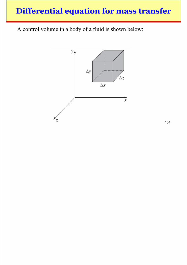
Differential equation for mass transfer
8/9/2019 SLides -1 TP
http://slidepdf.com/reader/full/slides-1-tp 104/112
104
A control volume in a body of a fluid is shown below:
Differential equation for mass transfer

8/9/2019 SLides -1 TP
http://slidepdf.com/reader/full/slides-1-tp 105/112
105
For the control volume
The net rate of mass transfer through the control volume may be
worked out by considering mass to be transferred across thecontrol surfaces.
( ) ( ) ( )
( ) ( )massof onaccumulatiof Ratenconsumptiomassof Rate
generationmassof Rateout massof Rateinmassof Rate
=−
+−
Differential equations for mass transferin terms of N A (molar units) [4]

8/9/2019 SLides -1 TP
http://slidepdf.com/reader/full/slides-1-tp 106/112
106
in terms of N A (molar units) [4]
∂
In rectangular coordinates
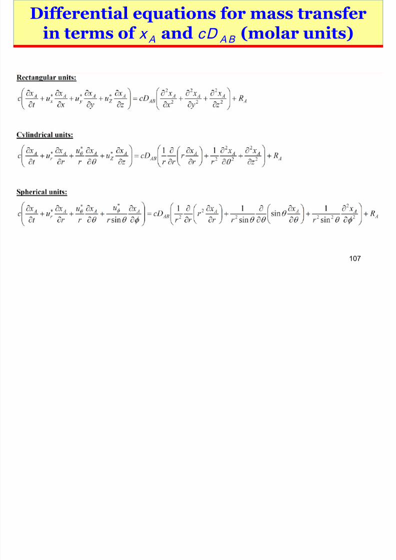
Differential equations for mass transferin terms of x A and cD AB (molar units)
8/9/2019 SLides -1 TP
http://slidepdf.com/reader/full/slides-1-tp 107/112
107
in terms of x A and cD AB (molar units)
Differential equation for mass transferin rectangular coordinates (mass units)

8/9/2019 SLides -1 TP
http://slidepdf.com/reader/full/slides-1-tp 108/112
108
in rectangular coordinates (mass units)
For the control volume
The net rate of mass transfer through the control volume may be
worked out by considering mass to be transferred across thecontrol surfaces.
A Az Ay Ax A r
z
n
y
n
x
n
t
+
∂
∂+
∂
∂+
∂
∂−=
∂
∂ ρ
Differential equations for mass transferin terms of j A [1]

8/9/2019 SLides -1 TP
http://slidepdf.com/reader/full/slides-1-tp 109/112
109
in terms of j Az [1]
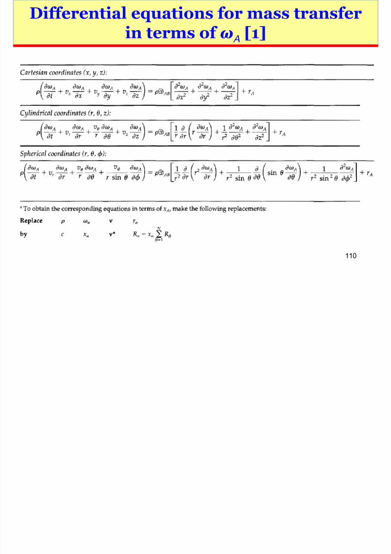
Differential equations for mass transferin terms of ωA [1]
8/9/2019 SLides -1 TP
http://slidepdf.com/reader/full/slides-1-tp 110/112
110
in terms of ωA [1]
Application of general mass balanceequations

8/9/2019 SLides -1 TP
http://slidepdf.com/reader/full/slides-1-tp 111/112
111
equations
Apply the general continuity equations described in the previous slides for various systems described in theterm.
Think other situations such as falling film problemdiscussed in Chapter 2 of the text [1] and develop themodel differential equations.
References[1] Bird, R.B. Stewart, W.E. Lightfoot, E.N. 2002. Transport Phenomena. 2nd ed. John
8/9/2019 SLides -1 TP
http://slidepdf.com/reader/full/slides-1-tp 112/112
[ ] , , g , pWiley & Sons, Inc. Singapore.
[2] Geankoplis, C.J. 1999. Transport processes and unit operations. 3rd ed. Prentice-Hall
International, Inc.[3] Foust, A.S.; Clump, C.W.; Andersen, L.B.; Maus, L.; Wenzel, L.A. 1980. Principles
of Unit Operations. 2nd ed. John Wiley & Sons, Inc. New York.
[4] Welty, J.R.; Wicks, C.E.; Wilson, R.E.; Rorrer, G.L. 2007. Fundamentals ofmomentum, heat and mass transfer. 5th ed. John Wiley & Sons, Inc.
[5] Poling, B.E.; Prausnitz, J.H.; O’Connell, J.P. 2000. The properties of gases andliquids. 5th ed. McGraw-Hill.
[6] Lide, D.R. 2007. CRC Handbook of Chemistry and Physics. 87th ed. CRC Press.
[7] Koretsky, M.D. 2013. Engineering and chemical thermodynamics. 2nd ed. John Wiley& Sons, Inc.
[8] Cengel, Y.A. (2003). Heat transfer: A practical approach. 2nd ed. McGraw-Hill.
[9] Staff of research and education association. The transport phenomena problem solver:momentum, energy, mass. Research and Education Association.