slide: 1 topic 4 production and costs. slide: 2 the firm and its economic problem firm an...

Slide: 1

TOPIC 4

PRODUCTION AND COSTS

Slide: 2

The Firm and ItsEconomic Problem

Firm

An institution that hires productive resources and that organises those resources to produce and sell goods and services

A firm’s goal is to maximize profit subject to a budget constraint

Slide: 3

Opportunity Cost

Firms incur opportunity costs when they produce goods.

Opportunity cost of producing — the best alternative investment opportunity that the firm foregoes to produce a good or service

Look at it as the opportunity costs of the factors of production the firm employs (labor, capital, entrepreneurs)

Slide: 4

Opportunity Cost

Components of a firm’s opportunity cost

Explicit costs (money costs)

The amount paid for factors of production

Implicit costs (non-money costs)

The value of foregone opportunities.

The firm incur implicit costs when it: uses its own capital uses its owner’s time or financial resources

Slide: 5

Opportunity Cost

Cost of Capital

Economic depreciation is the change in the market price of a durable input over a given time period (not the same as accounting depreciation).

Interest is the funds used to buy capital that could have been used for some other purpose.

Implicit rental rate is the income that the firm forgoes by using the assets itself and not renting them to another firm — the same as economic depreciation and interest costs.

Slide: 6

Opportunity Cost

Cost of Owner’s Resources

The income that the owner could have earned in the best alternative job.

Normal profit is the expected return for supplying entrepreneurial ability.

Slide: 7

Economic Profit

Economic Profit

A firm’s total revenue minus its opportunity costs.

Not the same as accounting profit.

Slide: 8

The Firm and Its Economic Problem

The Firm’s Constraints

Three features of its environment limit the maximum profit a firm can make. They are: Technology

Information

Market

Slide: 9

The Firm and Its Economic Problem

Technology Constraints A firm’s resources and the available technology limit its

production.

Information Constraints The cost of coping with limited information itself limits profit.

Market Constraints Willingness to pay of its customers and by the prices and

marketing efforts of rival firms.

Willingness of people to work for and invest in the firm.

Slide: 10

Technology and Economic Efficiency

Technological efficiency

Occurs when it is not possible to increase output without increasing inputs

Economic efficiency

Occurs when the cost of producing a given output is as low as possible

Slide: 11

Technological and Economic Efficiency

While technological efficiency depends only on what is feasible, economic efficiency depends on the relative cost of resources.

The economically efficient method is the one that uses the smallest amount of a more expensive resource and a larger amount of a less expensive resource.

Slide: 12

Information and Organisation

Organization of resources within the firm has a direct relation to the ability of the firm to achieve efficient outcomes

Command systems are based upon a managerial hierarchy.

Incentive systems are market-like mechanisms that firms create within their organisations. These systems are designed to strengthen incentives

and raise productivity.

Slide: 13

The Principal-Agent Problem

Principal-agent problem

The problem of devising compensation rules that induce an agent to act in the best interest of the principal

Three methods of attenuating the principal-agent problem are: Ownership Incentive pay Well-specified contracts

Slide: 14


Ownership

By assigning a manager or worker ownership of a business, it is sometimes possible to induce a job performance that increases the firm’s profits.

Example: Microsoft

Slide: 15


Incentive pay

Pay related to performance - are very common.

Based on a variety of performance criteria such as profits or production or sales targets.

Slide: 16


Well-specified contracts

Long-term contracts tie the long-term fortunes of managers and workers (agents) to the success of the principle(s) - the owner(s) of the firm, when the contract includes ownership features.

Short-term contracts can work as well when the contract is specified on the basis of the completion of specific tasks within specific time-periods

Note however, that specific contracts are costly (information, negotiation. Etc) to draw and are often too restrictive.

Slide: 17

The Types of Business Organisation

Sole Proprietorship a firm with a single owner

Partnership a firm with two or more owners who have unlimited

liability

Company a firm owned by one or more limited liability

stockholders

Slide: 18

The Pros and Cons of the Different Types of Firms

Proprietorship

Pros

Easy to set up

Simple decision making

Slide: 19


Proprietorship

Cons

Capital is expensive

Bad decision not checked by need for consensus

Owners entire wealth at risk

Ability to grow is restricted by availability to capital

Firm dies with owner

Slide: 20


Partnership

Pros

Easy to set up

Diversified decision making

Can survive withdrawal of partner

Slide: 21


Partnership

Cons

Achieving consensus may be slow and expensive

Owners entire wealth at risk

Withdrawal of partner may create capital shortage

Capital is expensive

Slide: 22


Company

Pros

Owners have limited liability

Large-scale, low-cost capital available

Professional management not restricted by ability of owners

Perpetual life

Long-term labour contracts cut labour costs

Slide: 23


Company

Cons

Complex management structure can make decision-making slow and expensive

Divorce of ownership and control highlights principal-agent problem

Slide: 24

Markets and the Competitive Environment

Economists identify four market types:

Perfect competition

Monopolistic competition

Oligopoly

Monopoly

Slide: 25


Perfect competition

Arises when there are many firms each selling an identical product, many buyers, and no restrictions on the entry of new firms into the industry.

Slide: 26


Monopolistic competition

A market structure in which a large number of firms compete by making similar buy slightly different products.

Product differentiation gives a monopolistically competitive firm an element of monopoly power.

Slide: 27


Oligopoly

A market structure in which a small number of firms compete.

Slide: 28


Monopoly

An industry that produces a good or service for which no close substitutes exists and in which there is one supplier that is protected from competition by a barrier preventing the entry of new firms.

Slide: 29


Concentration is an indicator variable for market power, but it is not a sufficient indicator

The Concentration Ratio Measures the percentage of the value of sales

accounted for by the four largest firms Range from 0 percent to 100 percent

Three-firm concentration ratio: measures the percentage of the value of sales

accounted for by the three largest firms in a market

Slide: 30


Three problems in the calculation and interpretation of concentration ratios

Market definition

Barriers to entry

Structure versus behaviour

Slide: 31

Market Structure

Characteristics competition competition Oligopoly Monopoly

Number of firms Many Many Few Onein market

Product Identical Differentiated Either identical No close or differentiated substitute

Barriersto entry None None Moderate High

Firm’s control None Some Considerable Considerableover price or regulated

Concentration ratio 0 Low High 100

Examples Wheat, meat office cleaning Automobiles, Local water car repairs chocolate bars distribution,

Perfect Monopolistic

Slide: 32

Firms and Markets

What determines whether markets or firms coordinate production?

Answer:Answer: Whichever is the economically efficient method.

Slide: 33

Why Firms?

Why firms are sometimes more efficient coordinators of economic activity?

Lower transactions costs

Economies of scale

Economies of scope

Economies of team production

Slide: 34

Why Firms?

Transactions costs The costs arising from finding someone with whom to

do business, of reaching an agreement about the price and other aspects of the exchange, and of ensuring that the terms of the agreement are fulfilled.

Coase and The Nature of the Firm

Slide: 35

Why Firms?

Economies of scale exist when the cost of producing a unit of a good falls as output increases.

Economies of scope exist when a firm uses specialised resources to produce a range of goods and services.

Team production A production process in which the individuals in a group

specialise in mutually supportive tasks.

Slide: 36

The Firm’s Time Horizon

The Short Run and the Long Run The short run is a period of time in which the quantity

of at least one input is fixed and the quantities of the other inputs can be varied. variable inputs and fixed inputs

The long run is a period of time in which the quantities of all inputs can be varied. The firm’s size can be selected

Slide: 37

Short-Run Technology Constraint

Increasing output in the short-run firms must increase the quantity of Labour

Total product is the total output produced.

Marginal product is the increase in total product that result from a one-unit increase in an input.

Average product is the total product divided by the quantity of inputs.

Slide: 38

Total Product, Marginal Product, and Average Product

Total Marginal Average Labour product product product (workers (hamburgers (hamburgers per (hamburgers per hour) per hour) additional worker) per worker)

a 0 0

b 1 25

c 2 60

d 3 80

e 4 90

f 5 95

Slide: 39



a 0 0

b 1 25

c 2 60

d 3 80

e 4 90

f 5 95

25

35

20

10

5

Slide: 40



a 0 0 -

b 1 25 25.00

c 2 60 30.00

d 3 80 26.67

e 4 90 22.50

f 5 95 19.00

25

35

20

10

5

Slide: 41

Attainable

Total Product Curve

0 1 2 3 4 5Labor (workers per day)

5

10

15TP

Unattainable

a

b

c

d

e fO

utpu

t (ha

mbu

rger

s pe

r ho

ur)

Slide: 42

Marginal Product Curve

Marginal product is also measured by the slope of the total product curve.

Increasing marginal returns occur when the marginal product of an additional worker exceeds the marginal product of the previous worker.

Slide: 43

Marginal Product Curve

Diminishing marginal returns Occur when the marginal product of an additional

worker is less than the marginal product of the previous worker

Law of diminishing returns As a firm uses more of a variable input, with a given

quantity of fixed inputs, the marginal product of the variable input eventually diminishes

Slide: 44

Marginal Product

Labour (workers per hour)

c

TP

Out

put (

ham

burg

ers

per

hour

)

Labour (workers per hour)

Mar

gina

l pro

duct

(ham

burg

ers

per

hour

per

wor

ker)

MP

d

The red highlightsthe point of diminishing returns

0 1 2 3 4 5

60

90

25

80

95

0 1 2 3 4 5

5

15

10

25

20

30

35

ef

Slide: 45

Average Product Curve

What does the average productWhat does the average product

curve look like?curve look like?

Remember that Marginals drag Remember that Marginals drag Averages!Averages!

Marginal grades in this course will Marginal grades in this course will influence where your average grade influence where your average grade

for the course isfor the course is

Slide: 46

Average Product

MP

AP

c

d

e

f

Maximumaverageproduct

Labour (workers per hour)0 1 2 3 4 5

5

15

10

25

20

30

35

26.67b

Mar

gina

l pro

duct

(ham

burg

ers

per

hour

per

wor

ker)

a

Slide: 47

Short-Run Cost

Total cost (TC) is the cost of all productive resources used by a firm.

Total fixed cost (TFC) is the cost of all the firm’s fixed inputs.

Total variable cost (TVC) is the cost of all the firm’s variable inputs.

Slide: 48

Short-Run Cost

Total cost (TC) is the cost of all productive resources used by a firm.

TC = TFC + TVC

TC TFC TVC

Q Q Q= +

OR ATC = AFC + AVC

Slide: 49

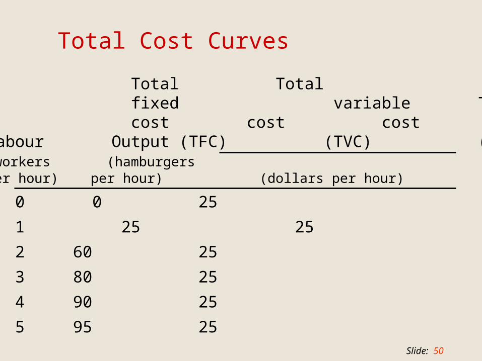
Total Cost Curves

Total Totalfixed variable Totalcost cost cost

Labour Output (TFC) (TVC) (TC)(workers (hamburgersper hour) per hour) (dollars per hour)

a 0 0

b 1 25

c 2 60

d 3 80

e 4 90

f 5 95

Slide: 50

Total Cost Curves



a 0 0 25

b 1 25 25

c 2 60 25

d 3 80 25

e 4 90 25

f 5 95 25

Slide: 51

Total Cost Curves



a 0 0 25 0

b 1 25 25 20

c 2 60 25 40

d 3 80 25 60

e 4 90 25 80

f 5 95 25 100

Slide: 52

Total Cost Curves



a 0 0 25 0 25

b 1 25 25 20 45

c 2 60 25 40 65

d 3 80 25 60 85

e 4 90 25 80 105

f 5 95 25 100 125

Slide: 53

TC

TVC

Total Cost Curves

TFC

TC = TFC + TVC

Output (hamburgers per hour)

Cos

t (do

llars

per

hou

r)

0 20 40 60 80 100

50

100

140

25

Slide: 54

Marginal Cost

Marginal cost is the increase in total cost that results from a one-unit increase in output.

It equals the increase in total cost divided by the increase in output.

Marginal costs decrease at low outputs because of the gains from specialisation, but it eventually increases due to the law of diminishing returns.

Slide: 55

Average Cost

Average fixed cost (AFC) is total fixed cost per unit of output.

Average variable cost (AVC) is total variable cost per unit of output.

Average total cost (ATC) is total cost per unit of output.

Slide: 56

Marginal Cost and Average Costs Total Total Average Average

fixed fixed Total Marginal fixed variable Total

cost cost cost cost cost cost cost

Labor Output (TFC) (TVC) (TC) (MC) (AFC) (AVC) (ATC)

(workers (hamburgers (cents per

per hour) per hour (dollars per hour) additional hamburgers) (cents per hamburgers)

a

b

c

d

e

f

0

1

2

3

4

5

0

25

60

80

90

95

25

25

25

25

25

25

0

20

40

60

80

100

25

45

65

85

105

125

—

100

42

31

28

26

—

80

67

75

89

105

—

180

108

106

117

132

80

57

100

200

400

Slide: 57

Marginal Cost and Average Costs


Cos

t (ce

nts

per

ham

burg

er) ATC = AFC + AVC

100

150

250

50

0 20 40 60 80 100

200

AVC

MC

ATC

AFC

Slide: 58

Long-Run Cost

Long-run cost The cost of production when a firm uses the

economically efficient quantities of labour and capital.

Long-run costs are affected by the production function.

Production function The relationship between the maximum output

attainable and the quantities of both Labour an Capital and the available state of technology.

Slide: 59

The Long-Run Average Cost Curve

The long run average total cost curve is derived from the short-run average total cost curves.

The segment of the short-run average total cost curves along which average total cost is the lowest make up the long-run average total cost curve.

Slide: 60

Fast Food

Long-Run Average Cost Curve


Ave

rage

cos

t (do

llars

per

ham

burg

er)

b

0 60 120 180 200 240

Factory

Deli

a

c

LRAC Curve

Slide: 61

Economies and Diseconomies of Scale

Returns to scale are the increases in output that result from increasing all inputs by the same percentage.

Three possibilities:

Constant returns to scale

Increasing returns to scale

Decreasing returns to scale

Slide: 62

Returns to Scale

Constant returns to scale

Technological conditions under which a given percentage increase in all the firm’s inputs results in the firm’s output increasing by the same percentage

Slide: 63

Returns to Scale

Increasing returns to scale

Technological conditions under which a given percentage increase in all the firm’s inputs results in the firm’s output increasing by a larger percentage

Slide: 64

Returns to Scale

Decreasing returns to scale

Technological conditions under which a given percentage increase in all the firm’s inputs results in the firm’s output increasing by a smaller percentage

Slide: 65

Constantreturns toscale

Increasingreturns toscale

SRACa

Output

Ave

rage

cos

t

Economies of ScaleLRAC

SRACb

Qo Q1Q2

Decreasing returns toscale

Slide: 66

Long-Run Costs

In the long-run all costs are variable because short-run fixed costs can be adjusted. So, the long-run average cost curve is the lower envelope of all the short run average cost curves

C

Q

ATC LRAC

Slide: 67

Economies of Scale

LRAC

C

QQ*

Economies of Scale

Diseconomies of Scale

LRAC decliningLR

AC

incr

easin

g

slide: 1 topic 4 production and costs. slide: 2 the firm and its economic problem firm an...

Documents