slicing up the san francisco bay area: block kinematics...
TRANSCRIPT
JOURNAL OF GEOPHYSICAL RESEARCH, VOL. ???, XXXX, DOI:10.1029/,
Slicing up the San Francisco Bay Area: Block
kinematics and fault slip rates from GPS-derived
surface velocitiesM. A. d’Alessio,
1,3I. A. Johanson,
1R. Burgmann,
1
D. A. Schmidt,2
and M. H. Murray1
Please cite as:d’Alessio, M. A., Johanson, I. A., Burgmann, R., Schmidt, D. A., and M. H. Mur-
ray. Slicing up the San Francisco Bay Area: Block kinematics and fault slip ratesfrom GPS-derived surface velocities. J. Geophys. Res., 110, doi: 10.1029/2004JB003496,2005. in press
M. A. d’Alessio, Department of Earth and Planetary Science, University of California, Berkeley,307 McCone Hall, Berkeley, CA 94720-4767, USA. ([email protected])
1Berkeley Seismological Laboratory,Berkeley, CA 94720-4760, USA
2Department of Geological Sciences,University of Oregon, Eugene, OR 97403,USA
3now at US Geological Survey, MenloPark, CA, USA
D R A F T May 19, 2005, 3:45pm D R A F T
X - 2 D’ALESSIO ET AL.: SLICING UP THE BAY AREA
Abstract. Observations of surface deformation allow us to determine the
kinematics of faults in the San Francisco Bay Area. We present the Bay Area
Velocity Unification (BAVU, “Bay-View”), a compilation of over 200 hor-
izontal surface velocities computed from campaign-style and continuous Global
Positioning System (GPS) observations from 1993-2003. We interpret this
interseismic velocity field using a 3-D block model to determine the relative
contributions of block motion, elastic strain accumulation, and shallow aseis-
mic creep. The total relative motion between the Pacific plate and the rigid
Sierra Nevada/Great Valley (SNGV) microplate is 37.9 ± 0.6 mm·yr−1 di-
rected towards N30.4W ± 0.8 at San Francisco (±2σ). Fault slip rates from
our preferred model are typically within the error bounds of geologic esti-
mates but provide a better fit to geodetic data (Notable right-lateral slip rates
in mm·yr−1: San Gregorio fault, 2.4 ± 1.0; West Napa fault, 4.0 ± 3.0;
zone of faulting along the eastern margin of the Coast Range, 5.4 ± 1.0;
and Mount Diablo thrust, 3.9 ± 1.0 of reverse-slip and 4.0 ± 0.2 of right-
lateral strike-slip). Slip on the northern Calaveras is partitioned between both
the West Napa and Concord/Green Valley fault systems. The total conver-
gence across the Bay Area is negligible. Poles of rotation for Bay Area blocks
progress systematically from the North America-Pacific to North America-
SNGV poles. The resulting present-day relative motion cannot explain the
strike of most Bay Area faults, but fault strike does loosely correlate with
inferred plate motions at the time each fault initiated.
D R A F T May 19, 2005, 3:45pm D R A F T
D’ALESSIO ET AL.: SLICING UP THE BAY AREA X - 3
1. Introduction
The San Francisco Bay Area hosts a complex plate boundary fault system with large,seismogenic faults that pose significant hazard to the local urban population. Faults inthe Bay Area are predominantly locked at the surface while steady plate-boundary motioncontinues to deform the surrounding crust. Monitoring this surface deformation allows usto determine block offset and strain accumulation along the faults. Geodetic monitoring offaults in the Bay Area has been a major effort of the scientific community since Reid firstformulated the elastic rebound theory [Reid , 1910]. The development of modern surveytechniques such as the Global Positioning System (GPS) allows enhanced measurementprecision. A number of studies have reported the results of GPS deformation fields andtheir estimates of the slip distribution on Bay Area faults [Savage et al., 1998; Freymuelleret al., 1999; Savage et al., 1999; Murray and Segall , 2001; Prescott et al., 2001]. Studieshave also used combinations of GPS and terrestrial geodetic measurements to determinedistribution of aseismic creep at depth on the Hayward [Burgmann et al., 2000; Schmidtet al., 2004] and Calaveras [Manaker et al., 2003] faults.
We present a compilation of GPS measurements for the Bay Area showing the inter-seismic velocity field from 1993-2003. We then interpret these velocities using a three-dimensional block model that considers the motion of regional crustal blocks and elasticstrain accumulation about block-bounding faults. We evaluate deformation at a range ofscales, including global tectonics, Bay Area wide deformation, the details of fault geome-try, and fault connections on the scale of kilometers.
2. GPS Data and Processing
2.1. Data
The Bay Area Velocity Unification (BAVU, pronounced “Bay-View”) includes campaignGPS data collected by six different institutions (U.C. Berkeley; U.S.G.S.; Stanford; U.C.Davis; U. Alaska, Fairbanks; CalTrans) from 1993 - 2003. UNAVCO archives all of theraw campaign data (http://archive.unavco.org) and the NCEDC archives the continuousBARD network (http://quake.geo.berkeley.edu/bard/). Transient deformation from the1989 Loma Prieta Earthquake decayed to near zero by 1993 [Segall et al., 2000], so thistime period captures relatively steady interseismic strain accumulation.
2.2. GPS Processing
We process GPS data using the GAMIT/GLOBK software package developed at theMassachusetts Institute of Technology and the Scripps Institution of Oceanography (SIO)[King and Bock , 2002; Herring , 2002]. We include five global stations from the Interna-tional GPS Service (IGS) network and four to six nearby continuous stations from theBARD network in each of our processing runs. We combine daily ambiguity-fixed, looselyconstrained solutions using the Kalman filter approach implemented by GLOBK [Her-ring , 2002]. We include data processed locally as well as solutions for the IGS and BARDnetworks processed by SOPAC at SIO (http://sopac.ucsd.edu/). Using the Kalman fil-ter, we combine daily solutions into monthly average solutions, giving each daily solutionequal weight. We then estimate the average linear velocity of each station in the networkfrom these monthly solutions. We translate and rotate the final positions and velocities
D R A F T May 19, 2005, 3:45pm D R A F T
X - 4 D’ALESSIO ET AL.: SLICING UP THE BAY AREA
of 23 IGS stations to their best fit values in the ITRF2000 No Net Rotation global ref-erence frame [Altamimi et al., 2002]. We then rotate the velocities into a stable NorthAmerica reference frame by solving for the best fitting relative pole of rotation shownfor the stations shown in Fig. 1. We scale the errors following the method used by theSouthern California Earthquake Center’s Crustal Motion Map version 3.0 team [SCECCMM 3.0, http://epicenter.usc.edu/cmm3/; Robert W. King, pers. comm., 2003]. Weadd white noise to the formal uncertainties of all stations with a magnitude of 2 mm·yr−1
for the horizontal components and 5 mm·yr−1 for the vertical component. To account for“benchmark wobble,” we add Markov process noise to the solutions with a magnitude of1 mm·yr−
12 . We also include velocities from SCEC CMM 3.0 [Shen et al., 2003] for several
sites in the Parkfield area to provide better coverage in central California.We show the BAVU GPS data for the Bay Area in Fig. 2 (also Table ES1*). We prefer
to visualize velocities in a local reference frame centered around station LUTZ (a BARDcontinuous site on the Bay Block, roughly at the BAVU network centroid). This referenceframe accentuates the gradient in deformation across the Bay Area. We subtract LUTZ’svelocity from all stations and propagate the correlations in uncertainty to calculate theerror ellipses.
2.3. No Outlier Exclusion
We include velocities for all stations that have at least four total observations spanningat least three years. At no point during the data processing or modeling do we excludedata that appear to be “outliers” based on initial assumptions about plate boundarymotion or model misfit. This ensures that the data truly dictate the model results, andthat scatter in the data is treated formally.
3. Block Modeling Methodology
In order to calculate slip along faults at depth from observed surface deformation,we must employ interpretive models. In the following sections, we discuss the physicalprocesses that are represented in our numerical model, including block offset, elastic strainaccumulation, and shallow interseismic creep.
3.1. Dislocation modeling
The San Andreas fault system forms the boundary between the Pacific (PA) plate andthe Sierra Nevada/Great Valley block (SNGV). Far from the fault, plate tectonic motionscontinue at a relatively constant rate. In the Bay Area, most plate-boundary faultsare presently locked near the surface during the interseismic period, causing the entireregion to deform elastically under the influence of this far-field plate motion. One wayto represent this system is to imagine that the fault itself is locked near the surface, butcontinues to slip at depth. Okada [1985] presents a useful formulation of the mathematicsof this relationship for finite fault segments (“dislocations”) in an isotropic, homogeneous,linearly elastic half space. Okada’s equations define the relationship between slip on agiven fault segment and surface displacement at each station. To uniquely define thisrelationship, one must specify the depth at which the fault transitions from the lockedbehavior near the surface to the deep, continuously slipping dislocation (i.e., the lockingdepth, LD). The transition could reflect thermally controlled onset of plastic flow [Sibson,
D R A F T May 19, 2005, 3:45pm D R A F T
D’ALESSIO ET AL.: SLICING UP THE BAY AREA X - 5
1982] or the transition from stable to unstable frictional sliding [Tse and Rice, 1986;Blanpied et al., 1995]. Because we use the dislocation as a proxy for steady plate motion,we treat the terms “long-term slip rate” and “deep slip rate” as synonyms.
3.2. Block Modeling
Block modeling is an extension of dislocation modeling, but with the additional physicalconstraint that dislocations form the boundaries of rigid plates, or “blocks” [e.g., Bennettet al., 1996; Murray and Segall , 2001; McCaffrey , 2002]. The amount of slip along eachdislocation is determined by the motion of the entire block, resulting in continuity ofslip on adjacent fault segments. Here we use an extension of the block modeling codeby Meade et al. [2002, also has a concise introduction to block modeling] and Meadeand Hager [2004, latest formulation of the methodology] that includes deformation fromshallow aseismic creep (see Sec. 3.3).
In block modeling, we define blocks on a spherical earth bounded by faults. Defining themodel geometry therefore requires more information than dislocation modeling becausethe location of fault connections must be known so that the faults form a continuousboundary around every block (Sec. 3.6). Each block rotates about a “rotation axis”passing through the center of the earth and intersecting the surface at a “pole of rotation”(sometimes referred to as an “Euler pole,” e.g. Cox and Hart [1986]).
For each block in the model, there are only three unknown parameters – the threecomponents of the angular velocity vector, Ω. The slip rates, s, of block bounding faultsare directly determined by the relative rotation of the surrounding blocks. We resolvethis relative motion onto the orientation of the fault that accommodates the motion,and the ratio between strike-slip, dip-slip, and tensile-slip (fault perpendicular motion)components is controlled exclusively by the fault orientation (s = f(Ω, fault strike, faultdip).
3.3. Surface Creep
Several faults in the Bay Area exhibit aseismic creep at depths shallower than LD [seeGalehouse and Lienkaemper , 2003]. To incorporate the effects of near-surface aseismiccreep on interseismic surface velocities, we include a shallow dislocation with uniform slipthat runs from the surface to a certain “transition depth” (TD). The TD must be ≤ LDbecause, by definition, the fault slips at a uniform rate below LD. The fault is locked atdepths between TD and LD. Because the detailed distribution of creep at depth is notwell known on all Bay Area faults, we assume the simplest case where TD=LD (the faultcreeps at one uniform rate from the surface to LD, where it transitions to its deep sliprate at all depths below LD). We explore the depth sensitivity of TD in Sec. 5.2. Theshallow dislocation representing aseismic creep is completely independent from the blockmotion and is permitted to slip at any rate slower or faster than the deep slip rate if thedata favor such behavior.
For segments where Galehouse and Lienkaemper [2003] observe surface creep magni-tudes less than 1 mm·yr−1, we do not solve for a shallow dislocation and keep the faultcompletely locked above LD. We only consider strike-slip motion on shallow dislocations,so c is a scalar.
BAVU includes more than 60 stations within 15 km of the Hayward fault, so we solvefor 4 different shallow dislocations along strike. However, it is not possible to reliably
D R A F T May 19, 2005, 3:45pm D R A F T
X - 6 D’ALESSIO ET AL.: SLICING UP THE BAY AREA
constrain the surface creep rate for some Bay Area faults with GPS data alone becausethe stations are not typically located within a few kilometers of the fault. We thereforeinclude the surface slip rates summarized in Galehouse and Lienkaemper [2003] as a prioriconstraints for the shallow slip rates with a priori uncertainties equal to the publisheduncertainties that include a random walk component. These uncertainties are sufficientlylarge such that the creep rate is determined largely by GPS data where stations are closeenough to a fault to resolve shallow slip.
3.4. Inverse Model
Combining block offset, elastic strain accumulation at block boundaries, and shallowaseismic creep, we solve the following equation in an inverse sense:
v(ri) = Ωi × ri −#Faults∑
f=1
[Gf
i · sf (Ωi)−Gfcreep,i · cf
](1)
where v is the predicted surface deformation rate, ri is the position of station i on earth,the first term on the right-hand side (cross product term) represents rigid rotation dueto the angular velocity of the block, the second term (summation term) represents elasticstrain related to fault slip on each segment. Gf
i and Gfcreep,i are Green’s functions relating
slip between the surface and fault f to deformation at station i for the deep dislocation(slip below LD) and shallow dislocation (between TD and the surface), respectively. Unlikethe deep slip rate, s, that is a function of the block rotation, Ω, the shallow creep rate, c,is a new model parameter that must be estimated. We solve for the value of Ω for eachblock and c for each creeping fault segment that predicts a velocity field most consistentwith our observations.
3.5. Inclusion of Global Data
We incorporate data from throughout the Pacific (PA) and North American (NA) platesto determine the total magnitude of relative motion that must be accommodated by BayArea faults. As long as the assumption that the plates behave rigidly in their interiorsis valid, global data far from faults provide valuable constraints. (Strictly speaking, wetreat the blocks as purely elastic. Because the blocks are so large, points near the plateinterior are virtually unaffected by elastic strain at the block boundaries. Hence, we referto block interiors as “rigid.”) Figure 1 shows the distribution of global stations that weinclude in our analysis.
Our block geometry includes a boundary between the SNGV and NA plates alongthe Eastern California Shear Zone (ECSZ) (Fig. 3). While the SNGV block is thoughtto behave “rigidly” [Argus and Gordon, 1991], the Basin and Range between easternCalifornia and the Colorado Plateau is an area of distributed deformation [Thatcher et al.,1999; Bennett et al., 2003]. We do not include data from within the Basin and Range, sowe are insensitive to the details of how deformation is distributed across it. Our ECSZboundary is therefore a proxy for the total deformation in the Basin and Range betweenthe SNGV and stable North America.
3.6. Fault Geometry
Recent geologic and geomorphic mapping efforts throughout the Bay Area, and espe-cially in the northern East Bay Area, provide new constraints on the details of fault geom-
D R A F T May 19, 2005, 3:45pm D R A F T
D’ALESSIO ET AL.: SLICING UP THE BAY AREA X - 7
etry. We define faults in our model using a combination of several data types: 1) Mappedsurface traces of faults; 2) Relocated microseismicity; 3) Topographic lineaments; and 4)Interpreted geologic cross sections. Figure 4 and Table ES2 show model fault segmentspresented in this manuscript and Table 1 describes the variations we discuss. We includemodels that range in complexity from intentionally oversimplified (such as “TwoPlate”)to those that are likely beyond the resolving power of our data (“Complex”).
4. Results
We evaluated nearly 100 different variations on fault geometry to determine the modelsmost consistent with the geodetic data and mapped faults. We report only a small subsetof these models, highlighting the key parameters that affect model fit. Changes in modelgeometry (including fault connections, location, orientation, LD, and TD) can affect theinferred fault slip rates greater than indicated by the formally propagated uncertaintiesfrom the inverse problem, which are typically < 1.5 mm·yr−1 at the 95% confidence level.For the range of reasonable geometries we test, the slip rates on almost all faults arewithin ±3 mm·yr−1 of the Preferred model, which we consider to be representative of theactual confidence interval of our slip rate estimates. For quantitative comparisons, werestrict our analyses to the formal uncertainties, but note that this variation should beconsidered when interpreting our results.
Figures 2 and 3 show observed and modeled GPS velocities for our Preferred model atthe scale of all the Bay Area and California, respectively. Overall, the model predictionsagree quite well with the observations and we capture many of the details of deformationacross the Bay Area. Examining the “residuals,” allows a more detailed comparison of thesystematic differences between observations and predictions for several model variations(Fig. 5).
We quantify the goodness of fit in terms of the χ2 and χ2/DOF statistics:
χ2 =#data∑c=1
(vmodel
c − vdatac
σc
)2
(2)
χ2/DOF =χ2
Ndata −Nmodel
(3)
where vmodelc and vdata
c are the predicted observed velocity components, and σc is the1σ uncertainty for each component of the input GPS velocities. The number of degreesof freedom (DOF) is defined by: Ndata, the number of GPS components used as inputdata (east and north component for each station, as well as any a priori constraints) andNmodel, the number of model parameters that we solve for in the inversion (pole of rotationlatitude, longitude, and rotation rate, as well as shallow creep rate for creeping segments).These statistics indicate how well the models fit the data within their uncertainty bounds.Lower values of χ2 indicate a better fit to the data. Increasing the number of modelparameters inevitably leads to better fits and lower total χ2. Dividing by the number ofdegrees of freedom (DOF) helps us compare models where we solve for a different numberof free parameters, but χ2/DOF ignores all correlations between parameters. Becausethese correlations change as model geometry changes, caution should be exercised inmaking strictly quantitative comparisons of models using χ2/DOF alone. Nonetheless,
D R A F T May 19, 2005, 3:45pm D R A F T
X - 8 D’ALESSIO ET AL.: SLICING UP THE BAY AREA
the statistics do provide a basis for qualitative comparisons. For uncorrelated modelparameters, a χ2/DOF of 1 indicates that, on average, all the predicted velocities areconsistent with the 1σ standard deviation of the input data. In Table 2, we present misfitstatistics for the models we discuss. We typically obtain χ2/DOF of 3-4, which is partlythe result of the χ2 statistic’s strong sensitivity to outliers.
In the following sections, we look in detail at the model results at a range of scales fromglobal motions to the details of fault connections and stepovers.
4.1. Global Plate Motion
To verify that our block model provides valid constraints on the total relative platemotion, we compare them with previously published results in Table ES3. Our estimatesof relative rotation axes incorporate the effect of elastic strain accumulation while theprevious studies of block motion typically exclude data from near plate boundaries. Toverify the quality of the BAVU global velocities, we use our block modeling code and theidentical subset of stations from Steblov et al. [2003]. Our results agree almost identicallyto their published results, though our propagated uncertainties are slightly smaller. Inour “TwoPlate” model, we include all 21 North American and 6 Pacific sites from BAVUthat are further than 100 km from a plate boundary. The pole of rotation from TwoPlateis 1.7 east, 1.3 north, and 0.5% slower than the Steblov et al. [2003] pole, but the changeis not significant at the 95% confidence level. The estimated pole from our “Preferred”model is about 0.9 east, 1.1 north, and 0.9% slower than the Steblov et al. [2003] pole.Globally, our data set and block modeling produce reasonable estimates of block motion.
Locally, the slight changes in the NA-PA rotation axis are insignificant. Table 3 showsthe predicted velocity at the Farallon Islands station 36 km west of the San Andreas fault(FARB). The predicted velocities for this Bay Area station differ by less than 0.1 mm·yr−1
and vary in azimuth by less than 0.1, despite differences in the NA-PA poles.
4.2. Sierra Nevada / Great Valley Block
The Sierra Nevada/Great Valley (SNGV) block is a rigid block that lies at the easternmargin of the Bay Area. The relative motion of the SNGV is not as well constrainedas larger plates because of the limited size of the block and relatively sparse data. Byincluding stations from throughout northern and southern California along with strainaccumulation near the block boundaries, our block model provides an improved constrainton the total PA-SNGV motion that must be accommodated by Bay Area faults. Table ES3shows our estimates of the relative motion between PA-SNGV and NA-SNGV comparedwith previous studies.
In general, the NA-SNGV pole tends to lie southwest of the Bay Area in the PacificOcean, as far as 90 from the NA-PA pole (Fig. 6). The NA-SNGV poles from previousstudies vary by > 50 in both longitude and latitude, and our results show a similarlybroad range due to slight variations in fault geometry and locking depth. These estimatesseem to lie along a consistent azimuth roughly perpendicular to the average fault strike inthe San Andreas fault system. The ideal station coverage for determining rotation axescovers a very broad area in all directions. The SNGV and other Bay Area blocks areelongate parallel to the San Andreas system and very narrow perpendicular to it. Theorientation of elongated error ellipses for these poles is related to the elongated shape ofthe blocks. This station geometry also results in a strong trade-off between the rotation
D R A F T May 19, 2005, 3:45pm D R A F T
D’ALESSIO ET AL.: SLICING UP THE BAY AREA X - 9
rate and distance of the poles of rotation from the Bay Area without strongly influencingpredictions of local surface deformation (e.g., Table 3).
The PA-SNGV pole is well constrained and located just west of Lake Superior, ∼ 20
from the NA-PA pole. Unlike NA-SNGV, formal uncertainties for this pole location are< 3, and the best-fit estimates vary by only ±6 for a wide range of model geometries.The pole for PA-SNGV is much less affected by the tradeoff between pole position androtation rate than the NA-SNGV pole.
4.3. Poles of Rotation of Bay Area Blocks
Focusing in on the Bay Area itself, we can examine rotation axes of smaller blocksbounded by Bay Area faults. Figure 6 shows the pole of rotation of each block relativeto North America. There is a systematic progression of the poles from west to east.In our Preferred model, the poles form a transition between the NA-SNGV and NA-PA poles. The Santa Cruz block, located adjacent to the Pacific plate, rotates abouta pole located near the NA-PA pole. On the other side of the Bay Area, the Coalingablock, located adjacent to the SNGV block, rotates about a pole located very close tothe NA-SNGV pole. These blocks near the margins of the Bay Area move very similarlyto the larger blocks that bound the region. Blocks within the Bay Area have rotationpoles relative to NA in between these poles, with blocks toward the eastern side of theBay Area tending to move more like NA-SNGV and blocks on the western side movingmore like NA-PA. This pattern holds for variations in locking depth and slight variationsin geometry on the Preferred model. For the Complex model, the poles of Bay Areablocks are still distributed between the NA-PA and NA-SNGV poles, but the east-westprogression breaks down slightly as many of the smaller blocks rotate about poles veryclose to the blocks themselves.
4.4. Slip Rates on Bay Area Faults
As described in Sec. 3.2, our block model uses GPS observations of surface deformationto calculate the best fitting deep slip rate from given block/fault geometries and lockingdepths. Here we present a general discussion about the effect of variations in locking depthon estimated slip rates (also see Sec. 5.1), and we present slip rates using our preferredlocking depths.4.4.1. Locking DepthFreymueller et al. [1999] described the strong trade-off between assumed locking depth
and calculated slip rate in dislocation models of the San Andreas system, making it chal-lenging to uniquely determine the slip rate on a given fault. We use the maximum depthof seismicity and surface heat flow to gain insight into the depth of the seismic/aseismictransition. Using this depth as a proxy for the geodetic LD helps reduce the ambiguityin determining slip rates. Earthquakes rarely occur below 20 km depth in the Bay Area,and the specific depth where faults become seismically quiet varies spatially throughoutthe region. Here we document temporal and spatial variation in the depth of seismicitythroughout the Bay Area in order to accurately determine the seismic/aseismic transitiondepths.
This transition is commonly quantified by the depth at which 95% of catalog seismicityoccurs above and 5% occurs below, or “D95.” Williams [2003] suggests that D95 accuratelyreflects the deepest extent of rupture in large earthquakes and presents the calculated
D R A F T May 19, 2005, 3:45pm D R A F T
X - 10 D’ALESSIO ET AL.: SLICING UP THE BAY AREA
values of D95 for Bay Area fault segments derived from the Northern California SeismicNetwork (NCSN) catalog. We perform a similar analysis on the high precision catalogof Waldhauser and Ellsworth [2002]. This catalog utilizes relative relocations that havevertical precision of less than about a hundred meters. We divide the Bay Area into adata-driven grid using the quadtree algorithm with a minimum grid cell size of 0.2 degrees[Townend and Zoback , 2001]. Figure 7 shows the depth of maximum seismicity for theentire duration of the catalog (1984-2001) and a movie in the electronic supplement showsthe time evolution of D95. Since LD is likely thermally controlled, we include heat flowobservations for reference. In both illustrations, grid cells are only filled with a color ifthere are more than 60 events during the time period indicated in the lower left. Thisnumber of events seems to produce consistent and stable values for D95 [Magistrale, 2002].
We do not utilize the D95 value as the locking depth for three fault segments. The Marinsegment of the San Andreas fault has essentially no seismicity, so we cannot calculate D95.The grid cells south and east of it both have locking depths close to 12 km. However, usinga locking depth of 15 km provides a better fit to the geodetic data. D95 on the Greenvillefault is very deep in the north near Mt. Diablo (18 km), but gets much shallower in gridcells to the south (other than the Geysers, these 3 grid cells have the shallowest D95 inthe Bay Area with values of 8-9 km). A much better fit is achieved if the 18 km lockingdepth is extended further south along all of the segments, including the fault along themargin of the Great Valley. Heat flow data are sparse in this region, but available datanear the Ortigalita fault range from 65− 85mWm2 [Lachenbruch and Sass , 1980], valuesmore consistent with a locking depth of 8-12 km, based on the relationships established byWilliams [1996]. The model preference for a deeper locking depth results in deformationover a broader region surrounding the single block boundary in our model, which couldbe indicative of a broader deformation zone in this region.4.4.2. Slip RatesDeep slip rates determined by our block model are reported in Fig. 5 and Tables 4 and
ES4. The total vector sum of relative motion accommodated by Bay Area faults in thePreferred model is 37.9 ± 0.6 mm·yr−1 oriented at N30.4W ± 0.8 in the central NorthBay and at N34.2W ± 0.8 in the central South Bay (Rate varies by 1-2 mm·yr−1 fromeast to west across the Bay Area, while azimuth varies by up to 8 from north to south).We report slip rate uncertainties at the 95% confidence level (2σ). The sum of best-fitslip rates ranges from 31.5-39.3 mm·yr−1 for the different fault geometries and lockingdepths we have explored. The Simple model consistently produces the lowest total sliprate. Within the Preferred model, the total slip is a strong function of assumed lockingdepth. The total best-fit slip rate ranges from 34.6-39.3 mm·yr−1 as we vary the lockingdepth over a range of 13 km.
We highlight the slip rates of a few key fault segments. Our model provides a robustestimate of slip on the San Gregorio fault. Because this fault is partly offshore in theBay Area it is very difficult to estimate a rate using independent dislocations and onshoredata. Our block model includes global stations to help constrain the motion of the Pacificblock relative to the Bay Area. The resulting slip rate on the San Gregorio fault from ourPreferred model is 2.4 ± 1.0 mm·yr−1 near the Golden Gate, with a slightly higher rateoff of Monterey Bay.
We include the West Napa fault in some models, as it may be the northern continuationof the Calaveras fault along a series of westward steps [J. Unruh, pers. comm., 2004]. We
D R A F T May 19, 2005, 3:45pm D R A F T
D’ALESSIO ET AL.: SLICING UP THE BAY AREA X - 11
find that its slip rate ranges from 3.4 - 7.4 mm·yr−1 across all models, with most modelsestimating slip rates near the lower end of this range. Models where 100% of the slipon the northern Calaveras fault transfers to the West Napa fault produce the higher sliprates. In our Preferred model it slips at 4.0 ± 3.0 mm·yr−1. This is the highest formaluncertainty for any deep slip rate in the inversion. In models where the West Napa faultand the Green Valley fault are both allowed to carry some of the Calaveras slip, theslip rates of the two faults sum to 9.5-11.0 mm·yr−1, depending on model geometry andlocking depth.
Models where we include a fault along the western margin of the Great Valley producesystematically better fits to the data than those that exclude this fault. This fault followsthe eastern front of the Coast Ranges, passing along the Ortigalita fault. We find a strike-slip rate of 5.4±1.0 mm·yr−1 in our Preferred model, and the rate typically varies between4-6 mm·yr−1.
4.5. Shallow Creep
Table ES5 shows the best-fit slip rates along dislocations that intersect the surface(surface creep) in our Preferred model. These rates typically vary by < 0.5 mm·yr−1
between most model geometries. Because data coverage is sparse in some areas, theformal uncertainties in creep rates are larger than for the deep slip rates. For the Haywardfault where BAVU has abundant near-fault velocities, the estimated creep rate has thesmallest uncertainty (1.2-1.4 mm·yr−1). The calculated creep rate variations there arequalitatively similar to the measurements from Lienkaemper et al. [2001] and are withinabout ∼ 1 mm·yr−1 of their observations even when the a priori constraints are removed.
In all cases except two, the best-fitting shallow slip rate is less than the best-fittingdeep slip rate. Forcing the creep rate on the southern Calaveras fault to be equal tothe deep slip rate increases the χ2/DOF by an insignificant 0.4%, as there is little datacoverage in this region. For the San Andreas fault south of San Juan Bautista (SegmentSanAndreas-SJB), the calculated shallow slip rate of ∼ 20.3 mm·yr−1 exceeds the deepstrike-slip rate of ∼ 16.4 mm·yr−1. The higher slip rate is favored in models without apriori constraints and produces a 4% reduction in misfit compared to a model where theshallow and deep segments are required to slip at the same rate. Johanson and Burgmann[2004] show that slip in this area is spatially complex.
5. Dependence of Slip Rate on Model Parameters
5.1. Locking Depth
The transition between creeping and locked behavior may not occur exactly at D95, butwe would expect the relative values of D95 to reflect the relative depth of this transition.To allow for the uncertainty in the absolute depth of the geodetic transition, we run themodel multiple times and shift LD uniformly up and down over a range of depths. Forexample, D95 for the northern Hayward fault is 12 km and D95 for the Concord fault is16 km. In our model runs, the LD of the Hayward fault is always 4 km shallower thanthe Concord fault, but we evaluate LD over the range of 3 - 17 km for the Hayward fault.
We show model misfit as a function of LD in Figure 8. The best fit comes when thelocking depths are about 5 km shallower than D95 for each segment. In model runs wherefaults are assigned a uniform LD, we find similar results. An 8 km uniform LD provides
D R A F T May 19, 2005, 3:45pm D R A F T
X - 12 D’ALESSIO ET AL.: SLICING UP THE BAY AREA
the best geodetic fit, even though it is also about 5 km shallower than the average 13km D95 for the entire Bay Area. Locking depths based on D95 produce insignificantlybetter model fit than the best-fitting uniform LD, but we prefer them because they arealso consistent with the independent seismicity data set.
Neither the uniform LD or deviations from D95 represent the absolute best statisticalfit to the data. Both approaches shift all locking depths uniformly up or down. Sincesome of the largest differences between observed and model GPS velocities occur near theSan Andreas fault in the southern Bay Area, Fig. 8 is dominated by the preference forshallow slip in that area. For example, fixing LD of the Santa Cruz Mountains segmentof the San Andreas fault to 5 km and keeping all other LD at D95 produces a bettermodel fit than shifting the entire model shallower by 5 km (star, Fig. 8; Sec.6.1). Whilesimultaneously inverting for both LD and slip rate would avoid such sensitivity, Prescottet al. [2001] found that such joint inversions produce poorer constraints on the slip rateand result in less geologically reasonable slip distributions.
5.2. Shallow Creep Transition Depth
Our treatment of shallow aseismic creep is oversimplified compared to faults in nature.Distributed slip models of the Calaveras and Hayward faults show a general pattern ofhigh aseismic slip rates near the surface with locked patches (very low aseismic slip rates)extending from a few kilometers depth to the seismic/aseismic transition (LD) [Manakeret al., 2003; Schmidt et al., 2004]. While the spatial resolution of our GPS data is nothigh enough to constrain the fine details of the aseismic slip distribution, we can explorethe general distribution of slip within three depth intervals along creeping faults: 1) ashallow dislocation representing aseismic creep from the surface to some depth, TD; 2)a locked patch between the depths of TD and LD; and 3) a deep dislocation below LD.In the models considered thus far, we assumed that TD=LD, resulting in only two depthintervals along the fault (1 and 3 from above). Here we evaluate a variation on thePreferred model where TD is a fixed depth of 5 km on all creeping faults, representingshallow creep restricted to the upper 5 km (Model “Preferred, TD=5”). The χ2/DOF is6% higher in “Preferred, TD=5” compared to the Preferred model. Slip rates for TD=5are almost all within the 95% confidence limits of the Preferred model, but there are somenotable differences. The shallower TD produces less slip at intermediate depths, so sliprates on the remaining dislocations must be higher to yield the same surface deformation.The resulting shallow slip rate is universally faster than for cases where TD=LD. Forcreeping segments of the San Andreas and Calaveras faults, the shallower TD producesslip rates 1-2 mm·yr−1 faster than when TD=LD. By assuming TD=5, the deep strike-sliprate on the central Calaveras fault increases from 12.9 to 15.0 mm·yr−1 and the slip onthe Hayward fault increases from 6.5 to 6.9 mm·yr−1. These slip increases are balanced bydecreased slip on several other Bay Area faults such that the total slip across the entireBay Area differs by less than 0.3 mm·yr−1 as TD varies. We find similar results in amodel where the shallow creep transition is exactly half-way between D95 and the surface(Model “Preferred, TD=D95/2”).
This relative insensitivity to the shallow creep transition depth is similar to the find-ings of Thatcher et al. [1997] who describe a geodetic inversion of slip during the 1906earthquake. They find that varying the depth extent of dislocations from 5-20 km causes<20% difference in the calculated slip on those elements. They also emphasize that even
D R A F T May 19, 2005, 3:45pm D R A F T
D’ALESSIO ET AL.: SLICING UP THE BAY AREA X - 13
though the calculated slip is uniform along the entire dislocation, the inversion is moresensitive to the slip rate in the shallow portions of the fault that are closer to the surfacegeodetic data.
We employ the assumption that TD=LD in our Preferred model because it producesthe lowest χ2/DOF . The improved fit may be due to the fact that slip rates between TDand LD are not exactly zero for the natural faults and that TD is likely to vary widelyamong the faults considered. By exploring a range of TD, we find that the shallow creeprates in our Preferred model are a lower bound, and the deep slip rates may vary fromthe Preferred model by 1− 2 mm·yr−1 for more complex distributions of shallow slip.
5.3. Fault-normal Slip Rate Constraints
The fault-normal slip rates from some previously published block models are sometimesof larger magnitude than geologically inferred slip rates [e.g., McClusky et al., 2001; Meadeet al., 2002]. From our own modeling, we find this is especially true when faults are sepa-rated by horizontal distance less than a few locking depths and there is limited GPS dataon the blocks. The inversion assigns high fault-normal slip rates of opposite signs to pairsof faults that are located close to one another. In such cases, the two slip rates balanceone another so that the total fault-normal slip satisfies the far-field constraint. Meadeand Hager [2004] refer to this phenomenon as “checkerboarding.” We found through trialand error that constraining the inversion to minimize the fault-perpendicular componenton a very small number of segments reduces these slip rate oscillations throughout theentire model. We add an a priori constraint to the fault perpendicular slip rate on threesegments whose strike is within 2.5 of the orientation of the PA-SNGV relative motion(northernmost Calaveras, northern Greenville, and northern Concord). We use a value of0 ± 3 mm·yr−1 for this constraint. These 1σ error bounds should allow convergence upto the total rate implied by previous geodetic studies for the entire Bay Area to occur onthese three segments if the data actually require it. We apply an identical constraint tothe Paicines fault because of its extremely close proximity to the much larger San An-dreas fault. All other segments in the model are unconstrained. Adding these constraintsincreases the total χ2 by only 0.5%. The constrained model does not cause a statisticallysignificant change in any of the model estimates. Figure ES1c shows that differencesbetween our Preferred model (with the constraint) and an identical geometry withoutthe constraint (“Preferred, Unclamped”) are negligible. We feel that the model withthese loose constraints produces physically reasonable slip rates without compromisingthe model fit or changing the qualitative interpretation of the results.
6. Discussion
6.1. Comparing the Models
Figure 9 shows the residuals for the three main model geometries we discuss. Theshading in Figure 9a shows the spatial distribution of the contribution to the total χ2
misfit. Larger values (darker colors) indicate that the model is doing a particularly poorjob of fitting the data in a certain area. The area around the epicenter of the 1989 LomaPrieta earthquake in the Santa Cruz Mountains has a systematic pattern in the residualvelocities and a high total misfit. Northeast of this section of the San Andreas fault(SAF) the data could be fit by a higher right-lateral slip rate and < 1 mm·yr−1 of fault
D R A F T May 19, 2005, 3:45pm D R A F T
X - 14 D’ALESSIO ET AL.: SLICING UP THE BAY AREA
perpendicular motion. Such an observation might indicate that accelerated postseismicdeformation along the fault persists at rates of ∼ 1 mm·yr−1 more than a decade afterthe 1989 earthquake. Stations near San Juan Bautista, also along the SAF, are fit poorly,though the orientations of residual velocities are not entirely systematic. Together, thetwo areas along the SAF in the southern Bay Area and a few strong outliers dominate theχ2 statistics. Models that improve the fit of those regions may have lower total χ2 even ifthey result in a worse fit throughout the rest of the model.
The shading in Figs. 9b-c and ES1 show where the weighted residuals (χ2) for eachmodel differ from the Preferred model. We calculate χ2 for the two components of eachGPS velocity in each model and then subtract this from χ2 in the Preferred model. Notehow changes to the geometry of the model in one location can alter the predicted velocitythroughout the model.
The Simple model (Fig. 9b) does a poor job fitting sites east of the Calaveras and SanAndreas faults in the southern Bay Area. Figure 3 illustrates that the fit to sites on theSNGV block is also poorer in the Simple model, with a systematic rotation of the predictedvelocities to the east (clockwise) of the data. The slip rate on the Mt. Lewis Trend andGreenville faults is left lateral for the Simple model, which is the opposite sense fromearthquake focal mechanisms in the region [e.g., Kilb and Rubin, 2002]. The systematicmisfit of GPS data and the opposite sense of slip are the motivation for including a “ValleyMargin deformation zone” in our Preferred model. Unruh and Sawyer [1998] suggest thatthe Greenville fault connects with the Ortigalita fault, a Holocene-active fault with bothvertical and strike-slip components that parallels the San Andreas fault system along theeastern margin of the Coast Ranges [Bryant and Cluett , 2000]. We extend a vertical faultthrough the trace of the Ortigalita fault, connecting to the San Andreas at the CarrizoPlain in the south and to the Greenville fault in the north. Geologic and geophysicalevidence supports the existence a major fault structure in this vicinity along the easternfront of the Coast Ranges [e.g., Wong and Ely , 1983; Wentworth and Zoback , 1989; Fuisand Mooney , 1990]. Seismicity, including the 1983 Coalinga event [Wong and Ely , 1983]suggest that a broad zone of faults may actually be accommodating the total relativemotion across the Coast Ranges, and not a single discrete structure. Because the GPSdata are sparse in this region, we are not able to differentiate between a single faultstructure and a zone of faults along the eastern Coast Ranges, nor are we sensitive to thedip of the structure or structures.
The Complex model (Fig. 9c) provides strong improvement to the model fit (8% reduc-tion in total χ2/DOF ), particularly the areas most poorly fit in the Preferred model nearLoma Prieta and San Juan Bautista. The Complex model has three blocks (Pleasanton,Sargent, and Paicines) added to the Preferred model’s 8 blocks. The Paicines block onlyhas a single GPS station on it and is therefore poorly constrained by the data. Improved fitto data around San Juan Bautista accounts for the greatest reduction in misfit – probablybecause we add two additional blocks (Sargent and Paicines) in this area (and thereforeadditional model parameters). Even though this model has the lowest misfit, the sparsedata coverage on these blocks and the known complexity of slip in this area suggest thatthe Complex model may not be the most accurate block model representation of the faultsystem in the southern Bay Area.
D R A F T May 19, 2005, 3:45pm D R A F T
D’ALESSIO ET AL.: SLICING UP THE BAY AREA X - 15
6.2. Comparison With Geologically-Determined Slip Rates
Numerous geologic investigations have determined long term average slip rates for BayArea faults during portions of the Holocene. Such studies provide essential input intoearthquake hazard assessment and an comprehensive summary of previous work has beencompiled for this purpose [Chapter 3 of Working Group on Northern California Earth-quake Probabilities , 2003, “WGCEP2002”]. In general, the geodetically observed slip ratesagree well with the values from WGCEP2002 (Tables 4 and ES4). Slight differences couldreflect a combination of errors in each data set or a real difference in the behavior of faultsduring the last decade compared to the last several thousand years. Both the Greenvillefault and the Green Valley/Concord fault system have slip rates higher than preferredbounds from WGCEP2002. More recent paleoseismological work by Sawyer and Unruh[2002] constrains the slip rate on the Greenville fault to 4.1± 1.8 mm·yr−1. This estimateagrees with the slip rate from our Preferred model (5.4 ± 0.6 mm·yr−1) within the errorbounds of each rate. The northern San Gregorio fault has a slip rate lower than the geo-logic bounds. In our model, all slip from the San Gregorio transfers to the Marin Segmentof the San Andreas fault, which also has a slip rate lower than the geologic bounds. TheHayward fault, Calaveras fault, and San Andreas fault from the Peninsula south all haveslip rates within the bounds described by WGCEP2002, but slightly lower than the mostprobable value. Most notably, none of our model variations produce slip rates on theHayward fault as high as the WGCEP2002 estimate. WGCEP2002 does not explicitlyconsider the effects of the West Napa fault as a possible extension of the Calaveras fault,while we find a slip rate of ∼ 3.5 mm·yr−1. We find a strike-slip rate for the Valley Margindeformation zone of 5.4 ± 1.0 mm·yr−1 in our Preferred model. WGCEP2002 does notestimate a slip rate for this region, but geologic investigations by Anderson and Piety[2001] show that the northern Ortigalita fault carries 0.5-2.5 mm·yr−1 of slip. The sliprate across the entire eastern Coast Ranges must be at least as high as the rate for thissingle structure.
A forward model of the WGCEP2002 fault parameters (long-term slip, fault width, andshallow locking ratio, R; “Preferred, WG02”) has χ2/DOF of 6.8, indicating that the sliprates from our Preferred model provide a substantially better fit to the BAVU geodeticdata.
6.3. Fault Connections: Northern Calaveras
Faults that are connected can transfer slip between one another and potentially rupturetogether in large earthquakes. Such connections can be complex and often are not mapped,but we must make inferences about how faults connect to define block boundaries. Whilethese inferences add non-uniqueness to our models, this feature of block modeling alsoallows us to test various scenarios of fault connections to see if they are consistent withour observed surface deformation rates.
The northern termination of the mapped Calaveras fault is an area where there is stillsignificant debate about which faults are connected to each other and where slip on theCalaveras gets transferred after the mapped trace terminates. Galehouse and Lienkaemper[2003] note that the nearly identical surface creep rates on the two systems imply thatthe Calaveras connects eastward to the Concord-Green Valley fault via a mechanicallyfavorable releasing step. Others [Unruh and Lettis , 1998; Unruh et al., 2002] suggest thatfold and fault geometry in the East Bay Hills indicate that the Calaveras steps westward
D R A F T May 19, 2005, 3:45pm D R A F T
X - 16 D’ALESSIO ET AL.: SLICING UP THE BAY AREA
with a restraining geometry, connecting to the West Napa fault and eventually transferringslip to the Rodgers Creek fault somewhere north of San Pablo Bay. Determining how slipis distributed between faults in the northern East Bay has important implications for theseismic hazard in these growing suburban areas. Using our block model, we focus on thisjunction and test a wide range of model geometries.
Overall, there is no substantive difference in model fit between models where the Calav-eras steps east versus west, though there are some scenarios where the east-stepping modelproduces a slightly smaller model misfit. Here we describe the effects of the two models“CalaverasWest” and “CalaverasEast,” which are both based on the Preferred model.
Forcing the Calaveras to transfer all slip to the west (CalaverasWest) brings slip onthe Calaveras system geographically closer to the Hayward/Rodgers Creek system. Thedeformation gradient in the GPS data near these two fault systems limits the combinedslip that can be accommodated by locked faults. When the two fault systems are closetogether, there is a tradeoff where more slip on the Calaveras/West Napa system requiresless slip on the Hayward/Rodgers Creek system. Slip on the Hayward fault in the Calav-erasWest model is 5.2 mm·yr−1, well below the ∼ 9 mm·yr−1 geologic slip rate estimatedfrom offset stream channels. The χ2/DOF for CalaverasWest is 2.0% higher than thePreferred model, but CalaverasWest affects the fit to stations as far away as Parkfield(Fig. ES1a).
CalaverasEast produces a higher slip rate on the Hayward fault of about 7.5 mm·yr−1,but also allows for 10.0 mm·yr−1 on the Green Valley fault because the Green Valley faultcarries the combined slip from both the northern Calaveras fault and the Valley Margindeformation zone. The χ2/DOF of the CalaverasEast model is 0.8% higher than thePreferred model and only affects the fit to GPS data in the northern Bay Area near wherethe model geometry differs.
Our Preferred model allows Calaveras slip to transfer both east and west. In it, sliprates are about half-way between the two scenarios CalaverasWest and CalaverasEast.Other model geometries that include the Mount Lewis trend, exclude the Valley Margindeformation zone, or use slightly different fault geometries have similar results.
Despite the fact that there are a number of GPS stations in the area of interest, itmay never be possible to distinguish between these different scenarios using geodetic dataalone. The West Napa and Green Valley faults are located < 10 km apart, similar tothe geodetic locking depth. It is difficult to distinguish between two elastic dislocationsburied about 15 km below the surface and spaced only 10 km apart. The added constraintfrom block offset could help distinguish between the two faults, especially as the detailsof shallow creep on the Green Valley fault are determined more precisely.
6.4. Dipping faults
All fault segments in our model are vertical, and in this section we discuss the technicaland conceptual limitations to using dipping faults in a block model based on dislocationtheory.
For vertical faults throughout all our models, we allow for the faults to open or theblocks to converge as a proxy for dip-slip faulting. This “tensile-slip” component (TableES6) accurately represents the total block motion, but the symmetric strain accumulationabout a vertical fault is not a perfect analog for dipping faults. The differences between
D R A F T May 19, 2005, 3:45pm D R A F T
D’ALESSIO ET AL.: SLICING UP THE BAY AREA X - 17
dip-slip and tensile-slip are pronounced for vertical deformation, but the differences areminor when only modeling horizontal components of GPS velocity.
Because thrust faulting may be important locally in the eastern Bay Area, we explorea variation on the Preferred model that includes dipping Mount Diablo and Mount Osothrust faults (“Preferred, Thrust”). The χ2/DOF for “Preferred, Thrust” is just 0.2%higher than the Preferred model and all slip rates are within 0.2 mm·yr−1 of the Preferredmodel.
All of our model geometries produce convergence across the Mount Diablo fault. Vari-ations on the Simple and Complex models that include a dipping Mount Diablo faultfind it has a reverse-slip of 2.7 and 5.7 mm·yr−1, respectively. In the “Preferred, Thrust”model, we find 3.9±1.0 mm·yr−1 of reverse-slip along with 4.0±0.2 mm·yr−1 of strike-slipacross the fault. The reverse component is within the 1.3-7.0 mm·yr−1 range determinedfrom restorations of geologic cross sections [Unruh and Sawyer , 1997]. The ratio betweenstrike-slip and horizontal shortening components depends on fault strike, but the totalmagnitude of the slip vector does not. The dip-slip magnitude is particularly sensitiveto fault dip because horizontal shortening is projected onto the dipping fault. We use adip of 38N for the Mount Diablo thrust, based on the 30 − 45 range in WGCEP2002.Because of the Mount Diablo thrust system’s role of transferring slip from the Greenvillefault to the Concord/Green Valley system in our model, it must carry several mm·yr−1
of slip consistent with block motion. A substantial portion of this slip must be strike-slipdeformation because the thrust system’s average strike is not perfectly perpendicular tothe relative block motion that it must accommodate.
6.5. Convergence in the Coast Ranges
Perfect transform faulting can occur when the rotation axes for a sequence of blocks arelocated at the same point but have different rates. Faulting will only be pure strike-slipeverywhere if all of the block boundaries are parallel to the small circle path of the relativemotion vector and parallel to one another (so that they never intersect). The situation inthe Bay Area meets neither of these conditions perfectly – the rotation axes of Bay Areablocks follow a systematic progression between the NA-PA and NA-SNGV blocks, andthe faults in the system are rarely parallel to one another. Abundant folds and thrustfaults roughly parallel to the San Andreas system suggest that pure strike-slip motion onthe major Bay Area faults does not accommodate all of the plate boundary motion. Weuse our block model to constrain the magnitude and location of any fault-perpendicularconvergence.
Savage et al. [1998] and Savage et al. [2004] determine the regional strain field in theBay Area. They find that the Bay Area as a whole undergoes an insignificant amount ofareal dilatation. They identify localized zones where contraction would give rise to thrustfaulting such as the region around the 1989 Loma Prieta rupture..
In contrast, some authors suggest that Bay Area GPS data require a small component offault-normal contraction between the SNGV block and the Bay Area. Prescott et al. [2001]analyze a profile between Point Reyes and Davis and find∼ 3.8±1.5 mm·yr−1 of shorteningover a 25-km-wide zone localized at the margin of the Great Valley. For a similar timespan and data covering a larger range of latitudes in the Bay Area, Murray and Segall[2001] find ∼ 2.4 ± 0.4 mm·yr−1 of contraction accommodated over a similarly narrow(<15km) zone. Freymueller et al. [1999] present data from further north and conclude
D R A F T May 19, 2005, 3:45pm D R A F T
X - 18 D’ALESSIO ET AL.: SLICING UP THE BAY AREA
that shortening must be < 1− 3 mm·yr−1. Pollitz and Nyst [2005] fit regional GPS datawith a viscoelastic model and find 3 mm·yr−1 of shortening perpendicular to a modelboundary oriented N34W. Additional campaign GPS observations since the publicationof those papers reduced the scatter in the data. Here we discuss new constraints on themagnitude of convergence in the Bay Area and the area over which it is accommodated.
Several of the previous observations of convergence in the Coast Ranges were based onthe presentation and interpretations of profiles across the plate boundary, such as we showfor BAVU in Fig. 10 [e.g., Fig. 2 of Murray and Segall , 2001; Fig. 5 of Prescott et al.,2001; Fig. 4 of Savage et al., 2004]. These plots show the two horizontal components ofGPS velocity projected onto a coordinate system with axes parallel and perpendicular toan “average” plate boundary orientation (usually parallel to the PA-NA relative motionand not PA-SNGV). The shape of the profile is highly dependent on the choice of theorientation used to define this average. Because the deformation field is projected ontoa single orientation, pure strike-slip motion on faults with a range of orientations canyield an apparent “fault normal contraction” signal. Figure 11 shows GPS data from theNorth Bay profile perpendicular to the San Andreas fault (N33.85W, Fig. 11a) and theazimuth of maximum shear strain from Savage et al. [2004] (N30W, Fig. 11b). Whenaccounting for the formal uncertainties, both profiles are statistically permissive of ascenario with no net convergence. The systematic pattern in both plots, however, impliesthat the variations are not random scatter. In the top profile, there is an abrupt step inthe data at the Green Valley fault, suggesting ∼ 2 mm·yr−1 of contraction between thePacific and SNGV accommodated near that structure. In the latter example, there is nonet plate-boundary normal motion between the Pacific and SNGV blocks (the data havenearly the same value on both ends of the profile). These two different projections of thesame data yield different conclusions about the magnitude and location of convergence inthe Bay Area – even though the profile orientation differs by only 4. This comparisonshould emphasize the hazard of representing spatially complex 2-D velocity data in anessentially 1-D illustration. The localized signal of contraction previously interpreted inthe Coast Ranges using these profiles is likely strike-slip motion of the Green Valley faultwhose orientation differs prominently from the average plate boundary. Evidence forconvergence cannot come from these “plate-boundary perpendicular” profiles.
More precise and rigorous measurements of the convergence across individual Bay Areafaults comes from comparing the orientation of vectors representing the relative motionbetween blocks (calculated in our model) and the orientation of individual mapped faultsaccommodating that motion [e.g., Argus and Gordon, 2001]. The vectors in Fig. 12 showthe orientation and magnitude of relative motion that is accommodated by faults in ourPreferred model assuming that the northeastern side of each fault is fixed. The relativemotion is, in general, nearly parallel to local fault strike. Resolving these vectors ontothe local fault orientation indicates the precise convergence that must be accommodated.These results are reported as “tensile-slip rates” in Table ES6. The bend in the SanAndreas fault at the Santa Cruz Mountains shows as much as 4.9± 0.6 mm·yr−1 of con-traction perpendicular to the segment (likely accommodated by a number of thrust faultsalongside the San Andreas fault). In general, motions east of the Bay are slightly clockwiseof the faults, indicating convergence across the block boundaries, which is balanced by aslight extensional component west of the Bay. The magnitude of convergence increasesfrom 0.1 ± 1.0 mm·yr−1 along the northern Hayward fault to 1.1 ± 1.0 mm·yr−1 on the
D R A F T May 19, 2005, 3:45pm D R A F T
D’ALESSIO ET AL.: SLICING UP THE BAY AREA X - 19
southernmost segment of the Hayward fault (Hayward 4). The segment connecting theHayward and Calaveras faults that roughly parallels the seismicity beneath Mission Peak(Hayward South) has 3.0± 1.0 mm·yr−1 of convergence. Along the eastern margin of theCoast Ranges, the Valley Margin deformation zone converges by 2.7± 0.8 mm·yr−1. TheConcord/Green Valley system requires a similar magnitude of convergence, but is locatedso close to the West Napa fault that the elastic model would probably not be able todistinguish between deep tensile-slip on the two faults (e.g., Sec. 5.3). We therefore treatthe Concord/Green Valley and West Napa fault systems together and find a statisticallyinsignificant 1.9±3.0 mm·yr−1 of convergence. The San Gregorio fault and Marin segmentof the San Andreas fault both show minor extension, with 2.9±0.6 and 1.9±0.6 mm·yr−1,respectively. It is not possible to determine if this motion is accommodated onshore oroffshore because of the sparse data west of these faults. Either way, this slight extensionis required to satisfy the total PA-SNGV relative motion. We therefore agree with theassertion by Savage et al. [2004] that while there are localized zones of convergence relatedto fault geometry, the geodetic data do not show evidence of measurable net convergenceacross the Bay Area.
6.6. Implications for fault system development
What does the systematic progression of poles of rotation from west to east shownin Fig. 6 tell us about the evolution and behavior of the Bay Area faults? There aretwo possibilities: 1) The rotation axes reflect the existing geometry of the faults. Blocksmerely move in a manner that is kinematically and mechanically favorable, given theorientation of pre-existing weaknesses in the area; or 2) Active faults are oriented at anoptimal angle to the far-field motion of the plates that drive them (to produce pure strike-slip faulting, for example) [Wesnousky , 1999]. Faults that are less optimally orientedmight be abandoned over time. Distinguishing the relative contributions of these twoend-member processes is beyond the scope of this work, but we can discuss the latteroption. Some faults in the Bay Area such as the San Andreas are oriented parallel withpresent day PA-NA motion, despite the fact that the plate boundary that should exerta controlling influence on the Bay Area is between the Pacific and SNGV blocks [e.g.,Argus and Gordon, 2001, W. Lettis, pers. comm., 2004]. The orientation of these faultscould be inherited from a time when the SNGV block moved more closely with NorthAmerica. Figure 12a shows the geometry of the San Andreas fault system comparedwith small circle traces parallel to the relative motion of the PA-NA and PA-SNGV.Faults parallel to the PA-SNGV relative motion show up as horizontal lines in this mapprojection. Few, if any, of the faults in the Bay Area are horizontal over much of theirextent. Most notably, almost the entire San Andreas fault is rotated counter-clockwise by∼ 5 from the ideal PA-SNGV motion (with the Santa Cruz Mountains segment rotated> 20 away). It is, in fact, roughly parallel with the predicted PA-NA motion from ourPreferred model. The central Calaveras, central Greenville, Concord, and Ortigalita faultshave strikes approximately parallel to PA-SNGV motion. Other fault segments, such asthe southern Calaveras, the Green Valley, and San Gregorio faults strike as much as 10
clockwise of the present PA-SNGV motion. With the exception of the San Gregorio fault,faults striking parallel to or clockwise of PA-SNGV motion are east of the Bay. Thegeneral disagreement between fault strike and total plate-boundary motion suggests thatpresent-day plate motion cannot explain the orientation of active faults in the Bay Area.
D R A F T May 19, 2005, 3:45pm D R A F T
X - 20 D’ALESSIO ET AL.: SLICING UP THE BAY AREA
Wakabayashi [1999] shows a general progression where the oldest active faults in the BayArea initiated in the west while the youngest faults in the Bay Area are to the east(though he emphasizes that there are abundant exceptions to this trend, especially forfaults that appear to have been abandoned and are currently inactive that show a muchmore complex age distribution). We focus here on the active faults because those are theones that are relevant for rotation axes derived from active deformation measurements.Figure 13 explores the relationship between the orientation of plate motion in the past andthe timing of initiation for individual fault segments. We calculate the PA-SNGV motionby subtracting the Basin and Range motion [reference point ‘A’, Wernicke and Snow ,1998] from PA-NA motion [Atwater and Stock , 1998]. The exact timing of initiation formany of the faults is not constrained reliably enough to make any definitive conclusionsfrom this figure. However, the plate reconstructions emphasize that the relative motionbetween PA-SNGV has rotated by > 30 during the lifetime of many Bay Area faults,and that this range encompasses most of the range of fault strikes observed in the BayArea. In light of these dramatic changes in plate motion in the past, it is probably unwiseto make conclusions about fault system development from our present-day GPS-derivedrotation axes.
7. Conclusions
The interseismic velocities at over 200 Bay Area stations provide a comprehensive pic-ture of crustal deformation in the region. The block modeling approach enables us tointerpret these velocities at a wide range of spatial scales.
We constrain the motion of blocks in the Bay Area relative to adjacent global plates (NAand PA), as well as the SNGV microplate. Individual blocks within the Bay Area do notmove about identical poles of rotation of any of these major blocks as a “perfect transform”system, but instead have poles at intermediate locations that vary in a systematic patternfrom east to west across the Bay Area (Fig. 6). This pattern may have implications forthe development of the fault system.
Looking at the Bay Area region, we quantify the slip rates of individual faults. Weuse precise relocations of earthquakes to determine the maximum depth of seismicity asa proxy for the local seismic/aseismic transition. We find slip rates that are typicallywithin the uncertainty of geologic estimates (Table 4). We also document substantial slipon segments that have not been emphasized in previous studies. Models that include upto 4 mm·yr−1 of strike-slip on the West Napa fault north of San Pablo Bay provide almostidentical model fits to those that exclude this fault. In our Preferred model, we favorthis geometry because it is consistent with geologic evidence showing that some slip fromthe Calaveras fault is transferred westward, eventually connecting to the West Napa faultsystem. Adding a fault along the eastern margin of the Coast Ranges in our Preferredmodel produces lower misfit and a geologically reasonable slip sense (right-lateral) onthe Greenville fault. This fault, running parallel to the San Andreas through centralCalifornia carries as much as 5 mm·yr−1 of right-lateral slip. Poor data coverage near themodel fault segment prevent us from determining if the deformation is accommodatedby a single structure or a broad zone with many structures as might be implied by thedistribution of moderate thrust earthquakes within the Diablo and Coast Ranges. Whilesuch events imply a substantial component of fault-normal convergence in the region, the
D R A F T May 19, 2005, 3:45pm D R A F T
D’ALESSIO ET AL.: SLICING UP THE BAY AREA X - 21
BAVU geodetic data are fit best with negligible convergence across the Coast Ranges. Ourblock modeling approach provides one of the first geodetic constraints on the slip ratesof several other faults because we include global GPS data from the Pacific plate andthe physical constraint of coherent block motion. These faults include the San Gregoriofault (2.4 ± 0.5 mm·yr−1 right-lateral slip rate) and the Mount Diablo thrust (3.9 ± 0.5mm·yr−1 reverse slip and an almost equal magnitude of right-lateral strike-slip). Overall,we find that the slip rates we determine fit GPS data substantially better than the sliprates defined in WGCEP2002.
We explore the possibility that the northern Calaveras fault transfers its slip east tothe Concord/Green Valley fault, west to the West Napa fault system, or a combinationof the two. The data slightly favor the eastern step over the western step alone, but weprefer models where both connections are included because they most closely reproducethe geologically inferred slip rate on the Green Valley fault and the lowest total modelmisfit.
In block modeling, three-dimensional fault geometry and connectivity have a very strongimpact on the interpretation of surface deformation. While we systematically exploredan extremely wide range of model geometries in this work, we look forward to furthergeologic constraints on fault geometry in 3-D to improve the reliability of block models.The ability to iteratively explore these different block geometries and test their consistencywith geodetic data make the block modeling approach an excellent tool for understandingfault kinematics in the Bay Area.
Acknowledgments. Dozens of students at the University of California, Berkeley gen-erously volunteered their time to help collect high quality geodetic data throughout theBay Area. This material is based on work supported by USGS NEHRP external grant04-HQGR-0119 and a National Science Foundation Graduate Research Fellowship. Con-tinuous data from the BARD network and campaign GPS data collected by the U.S.Geological Survey were obtained from the Northern California Earthquake Data Center.We acknowledge SOPAC at U.C. San Diego for easy access to GAMIT processing resultsof global and regional networks. J. Beavan, Y. Bock, and J. Savage provided useful reviewsof the manuscript. Robert King provided suggestions on GPS error scaling methodology.Jeff Unruh helped us define the most realistic model geometry possible. We are gratefulto Brendan Meade for providing us his well documented block modeling code. BerkeleySeismological Laboratory contribution 05-04.
References
Altamimi, Z., P. Sillard, and C. Boucher, ITRF2000: A new release of the internationalterrestrial reference frame for earth science applications, J. Geophys. Res., 107 (B10),doi:10.1029/2001JB000,561, 2002.
Anderson, L. W., and L. A. Piety, Geologic seismic source characterization of the SanLuis-O’Neill area, eastern Diablo Range, California, Seismotectonic Report 2001-2,Bureau of Reclamation, 2001.
Argus, D. F., and R. G. Gordon, Current Sierra-Nevada North America motion from VeryLong Base-Line Interferometry - implications for the kinematics of the western UnitedStates, Geology, 19 (11), 1085–1088, 1991.
D R A F T May 19, 2005, 3:45pm D R A F T
X - 22 D’ALESSIO ET AL.: SLICING UP THE BAY AREA
Argus, D. F., and R. G. Gordon, Present tectonic motion across the Coast Ranges and SanAndreas fault system in central California, Geol. Soc. Amer. Bull., 113 (12), 1580–1592,2001.
Atwater, T., and J. Stock, Pacific-North America plate tectonics of the Neogene south-western United States: An update, Int. Geol. Rev., 40 (5), 375–402, 1998.
Bennett, R. A., W. Rodi, and R. E. Reilinger, Global positioning system constraints onfault slip rates in southern California and northern Baja, Mexico, J. Geophys. Res.,101 (B10), 21,943–21,960, 1996.
Bennett, R. A., B. P. Wernicke, N. A. Niemi, A. M. Friedrich, and J. L. Davis, Contempo-rary strain rates in the northern Basin and Range province from GPS data, Tectonics,22 (2, 1008), doi:10.1029/2001TC001,355, 2003.
Blanpied, M. L., D. A. Lockner, and J. D. Byerlee, Fault slip of granite at hydrothermalconditions, J. Geophys. Res., 100 (B7), 1995.
Bryant, W., and S. Cluett, Fault number 52b, Ortigalita fault zone, Los Banos Valley sec-tion, in Quaternary fault and fold database of the United States, ver 1.0, U.S. GeologicalSurvey Open File report 03-417, http://qfaults.cr.usgs.gov, 2000.
Burgmann, R., D. Schmidt, R. M. Nadeau, M. A. d’Alessio, E. Fielding, T. V. McEvilly,and M. H. Murray, Earthquake potential along the northern Hayward fault, California,Science, 289 (18 August 2000), 1178–1182, 2000.
Cox, A., and R. B. Hart, Plate tectonics: How it works, Blackwell Scientific Publications,Palo Alto, California, 1986.
Freymueller, J. T., M. H. Murray, P. Segall, and D. Castillo, Kinematics of the Pacific-North America plate boundary zone, northern California, J. Geophys. Res., 104 (B4),7419–7441, 1999.
Fuis, G. S., and W. D. Mooney, Lithospheric structure and tectonics from seismic re-fraction and other data, in The San Andreas fault system, California, edited by R. E.Wallace, U.S. Geological Survey Professional Paper 1515, pp. 207–236, 1990.
Galehouse, J. S., and J. J. Lienkaemper, Inferences drawn from two decades of alinementarray measurements of creep on faults in the San Francisco Bay Region, Bull. Seism.Soc. Amer., 93 (6), 2415–2433, 2003.
Herring, T. A., GLOBK, global Kalman filter VLBI and GPS analysis program, 2002.Johanson, I. A., and R. Burgmann, Complexity at the junction of the Calaveras and San
Andreas faults, J. Geophys. Res., in preparation, 2004.Kilb, D., and A. M. Rubin, Implications of diverse fault orientations imaged in relocated
aftershocks of the Mount Lewis, M-L 5.7, California, earthquake, J. Geophys. Res.,107 (B11), doi:10.1029/2001JB000,149, 2002.
King, R. W., and Y. Bock, Documentation for the GAMIT GPS analysis software, v.10.0,, Massachusetts Institute of Technology, Scripps Institute of Oceanography, 2002.
Lachenbruch, A. H., and J. H. Sass, Heat flow and energetics of the San Andreas faultzone, J. Geophys. Res., 85 (B11), 6185–6222, 1980.
Lienkaemper, J. J., J. S. Galehouse, and R. W. Simpson, Long-term monitoring of creeprate along the Hayward fault and evidence for a lasting creep response to 1989 LomaPrieta earthquake, Geophys. Res. Lett., 28 (11), 2265–2268, 2001.
Magistrale, H., Relative contributions of crustal temperature and composition to con-trolling the depth of earthquakes in southern California, Geophys. Res. Lett., 29 (10),2002.
D R A F T May 19, 2005, 3:45pm D R A F T
D’ALESSIO ET AL.: SLICING UP THE BAY AREA X - 23
Manaker, D. M., R. Burgmann, W. H. Prescott, and J. Langbein, Distribution of inter-seismic slip rates and the potential for significant earthquakes on the Calaveras fault,central California, J. Geophys. Res., 108 (B6), doi:10.1029/2002JB001,749, 2003.
McCaffrey, R., Crustal block rotations and plate coupling, in Plate boundary zones, AGUGeodynamics Series, vol. 30, edited by S. Stein and J. T. Freymueller, pp. 101–122,2002.
McClusky, S. C., S. C. Bjornstad, B. H. Hager, R. W. King, B. J. Meade, M. M. Miller,F. C. Monastero, and B. J. Souter, Present day kinematics of the Eastern CaliforniaShear Zone from a geodetically constrained block model, Geophys. Res. Lett., 28 (17),3369–3372, 2001.
Meade, B. J., and B. H. Hager, Block models of crustal motion in southern Californiaconstrained by GPS measurements, J. Geophys. Res., in review, 2004.
Meade, B. J., B. H. Hager, S. McClusky, R. E. Reilinger, S. Ergintav, O. Lenk, A. Barka,and H. Ozener, Estimates of seismic potential in the Marmara Sea region from blockmodels of secular deformation constrained by Global Positioning System measurements,Bull. Seism. Soc. Amer., 92, 208–215, 2002.
Murray, M. H., and P. Segall, Modeling broadscale deformation in northern Californiaand Nevada from plate motions and elastic strain accumulation, Geophys. Res. Lett.,28 (22), 4315–4318, 2001.
Okada, Y., Surface deformation due to shear and tensile faults in a half-space, Bull. Seism.Soc. Amer., 75 (4), 1135–1154, 1985.
Pollitz, F. F., and M. C. J. Nyst, A physical model for strain accumulation in the SanFrancisco Bay Region, Geophys. J. Int., 160, 302–317, 2005.
Prescott, W. H., J. C. Savage, J. L. Svarc, and D. Manaker, Deformation across thePacific-North America plate boundary near San Francisco, California, J. Geophys. Res.,106 (B4), 6673–6682, 2001.
Reid, H. F., The mechanics of the earthquake, in The California earthquake of April18, 1906: Report of the State Investigation Commission, vol. 2, Carnegie Institute ofWashington, Washington, D.C., 1910.
Savage, J. C., R. W. Simpson, and M. H. Murray, Strain accumulation rates in the SanFrancisco Bay Area, 1972-1989, J. Geophys. Res., 103 (B8), 18,039–18,051, 1998.
Savage, J. C., J. L. Svarc, and W. H. Prescott, Geodetic estimates of fault slip rates inthe San Francisco Bay Area, J. Geophys. Res., 104 (B3), 4995–5002, 1999.
Savage, J. C., W. Gan, W. H. Prescott, and J. L. Svarc, Strain accumulation across theCoast Ranges at the latitude of San Francisco, 1994-2000, J. Geophys. Res., 109 (B3),doi:10.1029/2003JB002,612, 2004.
Sawyer, T. L., and J. R. Unruh, Holocene slip rate constraints for the northern Greenvillefault, eastern San Francisco Bay Area, California: Implications for the Mt. Diablo re-straining stepover model, EOS, Trans. Amer. Geophys. Union, 83 (47), Abstract T62F–03, 2002.
Schmidt, D. A., R. Burgmann, R. M. Nadeau, and M. A. d’Alessio, Distribution of aseismicslip-rate on the Hayward fault inferred from seismic and geodetic data, J. Geophys. Res.,in review, 2004.
Segall, P., R. Burgmann, and M. V. Matthews, Time dependent triggered afterslip fol-lowing the 1989 Loma Prieta earthquake, J. Geophys. Res., 105, 5615–5634, 2000.
D R A F T May 19, 2005, 3:45pm D R A F T
X - 24 D’ALESSIO ET AL.: SLICING UP THE BAY AREA
Shen, Z.-K., et al., Southern California Earthquake Center Crustal Motion Map Version3.0, http://epicenter.usc.edu/cmm3/, 2003.
Sibson, R. H., Fault zone models, heat flow, and the depth distribution of earthquakesin the continental crust of the United States, Bull. Seism. Soc. Amer., 68, 1421–1448,1982.
Steblov, G. M., M. G. Kogan, R. W. King, C. H. Scholz, R. Burgmann, and D. I. Frolov,Imprint of the North American plate in Siberia revealed by GPS, Geophys. Res. Lett.,30 (18), doi:10.1029/2003GL017,805, 2003.
Thatcher, W., G. Marshall, and M. Lisowski, Resolution of fault slip along the 470-km-long rupture of the great 1906 San Francisco earthquake and its implications, J.Geophys. Res., 102 (B3), 5353–5367, 1997.
Thatcher, W., G. R. Foulger, B. R. Julian, J. Svarc, E. Quilty, and G. W. Bawden,Present-day deformation across the Basin and Range province, western United States,Science, 283, 1714–1718, 1999.
Townend, J., and M. D. Zoback, Focal mechanism stress inversions in southern Californiaand the strength of the San Andreas fault, in Proceedings of the Conference on TectonicProblems of the San Andreas Fault System, vol. 30, pp. 268–276, Stanford UniversityPublication, Geological Sciences, 2001.
Tse, S. T., and J. R. Rice, Crustal instability in relation to the depth variation of frictionalslip properties, J. Geophys. Res., 91 (B9), 9452–9472, 1986.
Unruh, J. R., and W. R. Lettis, Kinematics of transpressional deformation in the easternSan Francisco Bay region, California, Geology, 26, 19–22, 1998.
Unruh, J. R., and T. L. Sawyer, Assessment of blind seismogenic sources, LivermoreValley, eastern San Francisco Bay Region: Final technical report submitted to the U.S.Geological Survey, National Earthquake Hazards Reduction Program, award no. 1434-95-g-2611, 1997.
Unruh, J. R., and T. L. Sawyer, Paleoseismic investigation of the northern Greenvillefault, eastern San Francisco Bay Area, California: Final technical report submitted tothe U.S. Geological Survey, National Earthquake Hazards Reduction Program awardno. 1434-hq-97-gr-03146, , 1998.
Unruh, J. R., K. I. Kelson, D. Manaker, and A. Barron, Critical evaluation of the northerntermination of the Calaveras fault, eastern San Francisco Bay Area, California, Report1430, William Lettis and Associates, 2002.
Wakabayashi, J., Distribution of displacement on and evolution of a young transformsystem: The northern San Andreas fault system, California, J. Geophys. Res., 18 (B6),1245–1274, 1999.
Waldhauser, F., and W. L. Ellsworth, Fault structure and mechanics of the Hayward fault,California, from double-difference earthquake locations, J. Geophys. Res., 107 (B3),doi:10.129/2000JB000,084, 2002.
Wentworth, C. M., and M. D. Zoback, The style of late Cenozoic deformation at theeastern-front of the California Coast Ranges, Tectonics, 8 (2), 237–246, 1989.
Wernicke, B., and J. K. Snow, Cenozoic tectonism in the central Basin and Range: Motionof the Sierran-Great Valley block, Int. Geol. Rev., 40 (5), 403–410, 1998.
Wesnousky, S. G., Crustal deformation processes and the stability of the Gutenberg-Richter relationship, Bull. Seism. Soc. Amer., 89 (4), 1131–1137, 1999.
D R A F T May 19, 2005, 3:45pm D R A F T
D’ALESSIO ET AL.: SLICING UP THE BAY AREA X - 25
Williams, C. F., Temperature and the seismic/aseismic transition: Observations from the1992 Landers earthquake, Geophys. Res. Lett., 23 (16), 2029–2032, 1996.
Williams, C. F., Implications of the depth of seismicity for the rupture extent of futureearthquakes in the San Francisco Bay Area, U. S. Geol. Survey Open File Rep., 03-214,A1–A16, 2003.
Wong, I. G., and R. W. Ely, Historical seismicity and tectonics of the Coast Ranges-Sierrablock boundary: Implications to the 1983 Coalinga earthquakes, in The 1983 Coalinga,California earthquakes, edited by J. Bennet and R. Sherburne, California Division ofMines and Geology Special Publication 66, pp. 89–104, 1983.
Working Group on Northern California Earthquake Probabilities, Earthquake probabili-ties in the San Francisco Bay region: 2002 to 2031, U.S. Geol. Surv. Open File Rep.,03-214, 2003.
D R A F T May 19, 2005, 3:45pm D R A F T
X - 26 D’ALESSIO ET AL.: SLICING UP THE BAY AREA
50 mm yr-1
10 mm yr-1
KELY
STJO
BRMU
SCH2
THU1
BARNWES2
NRC1
GODEUSNO
ALGO
AOMLRCM6
NLIB
CHUR
DUBO
FLIN
MDO1
AMC2PIE1
PRDS
YELL
DRAO
WILL
WHITFAIR
THTITAHI
MKEAKOKB
CHAT
KWJ1
PA-NA
Figure 1. Observed global GPS velocities shown in a reference frame with stable NorthAmerica. Figure shows only stations included in modeling, but BAVU includes additionalglobal stations for reference frame stabilization. 95% confidence bound on Pacific-NorthAmerica relative pole of rotation for the Preferred model is shown as the very small ellipseto the right of the PA-NA label. 95% confidence ellipses on velocities.
D R A F T May 19, 2005, 3:45pm D R A F T
D’ALESSIO ET AL.: SLICING UP THE BAY AREA X - 27
LUTZ
BAVU Observations Model (Preferred)
20 mm yr -1
GMT 2004 Jul 16 16:22:20
0 30 km
Figure 2. The BAVU data set. Map of the San Francisco Bay Area with GPSvelocities from 1993-2003 relative to station LUTZ in the Bay Block. The map projectionis about the Pacific Plate–Sierra Nevada/Great Valley (PA-SNGV) pole of rotation, sovelocities along a small circle path predicted from the rotation axis of the PA-SNGVblock rotation show up as horizontal vectors. We compare observations (wider vectorswith 95% confidence error ellipses) with predictions from our Preferred model (narrow,darker vectors).
D R A F T May 19, 2005, 3:45pm D R A F T
X - 28 D’ALESSIO ET AL.: SLICING UP THE BAY AREA
VM
dz
CR
f
Santa C
ruz Block
EC
SZ
BAVU Observations
Preferred Model
Simple Model
100 km
30mm/yr
North
America
Block
Pacific
Block
Sierra Nevada/
Great Valley
Block
Coalinga B
lock
Figure 3. GPS observations within California, shown in a reference frame with stableNorth America (wide vectors with error ellipses) compared with model results (narrowvectors). Dark sinuous lines are Holocene active faults. Dotted grey lines show a repre-sentative model geometry from our Complex model that includes all segments. We labelselect blocks and faults outside the Bay Area. VMdz = Valley Margin deformation zone;ECSZ = Eastern California Shear Zone. Inset shows an enlargement of the area where thetwo models differ most in the northern section of the figure. Our Preferred model witha VMdz (darker vectors) fit the data better than models that exclude this fault (Simplemodel, white vectors).
D R A F T May 19, 2005, 3:45pm D R A F T
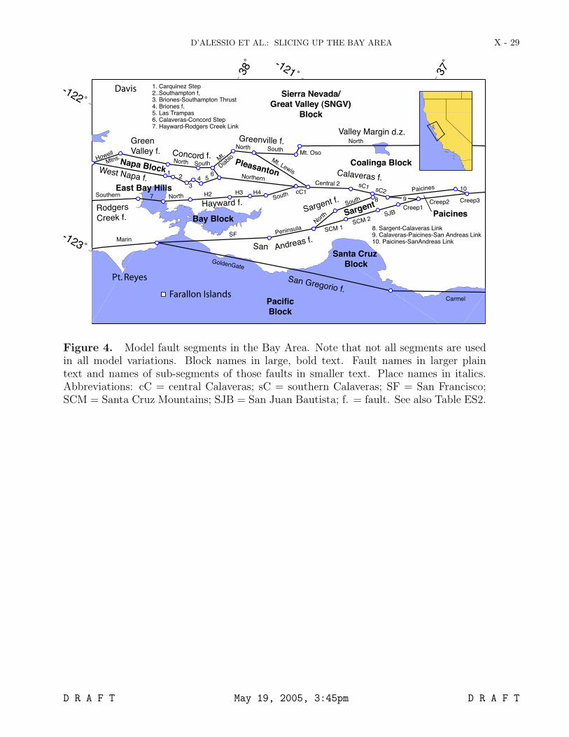
D’ALESSIO ET AL.: SLICING UP THE BAY AREA X - 29
Farallon Islands
Pt. Reyes
Davis
GoldenGate
North H2 H3 H4South
MarinSF Peninsula SCM 1
SJB
SCM 2
Creep1Creep2 Creep3
Paicines
Mt. OsoNorth South
North SouthM
t.
Dia
blo Mt. LewisNorthern
Central 2
cC1
sC1 sC2
Carmel
Howell
Mtns.
Southern
North
South
12
34 5
6
7
10
9
1. Carquinez Step2..Southampton f,3. Briones-Southampton Thrust4. Briones f.5. Las Trampas6. Calaveras-Concord Step7. Hayward-Rodgers Creek Link
8. Sargent-Calaveras Link9. Calaveras-Paicines-San Andreas Link10. Paicines-SanAndreas Link
North
8
San Gregorio f.
Hayward f.
Greenville f.
Rodgers
Creek f.
West Napa f.Calaveras f.
GreenValley f.
Valley Margin d.z.
Concord f.
San Andreas f.
Sargent f.
Pacific
Block
Bay Block
Santa Cruz
Block
Coalinga Block
Sierra Nevada/
Great Valley (SNGV)
Block
East Bay Hills
Napa BlockPleasanton
SargentPaicines
Figure 4. Model fault segments in the Bay Area. Note that not all segments are usedin all model variations. Block names in large, bold text. Fault names in larger plaintext and names of sub-segments of those faults in smaller text. Place names in italics.Abbreviations: cC = central Calaveras; sC = southern Calaveras; SF = San Francisco;SCM = Santa Cruz Mountains; SJB = San Juan Bautista; f. = fault. See also Table ES2.
D R A F T May 19, 2005, 3:45pm D R A F T
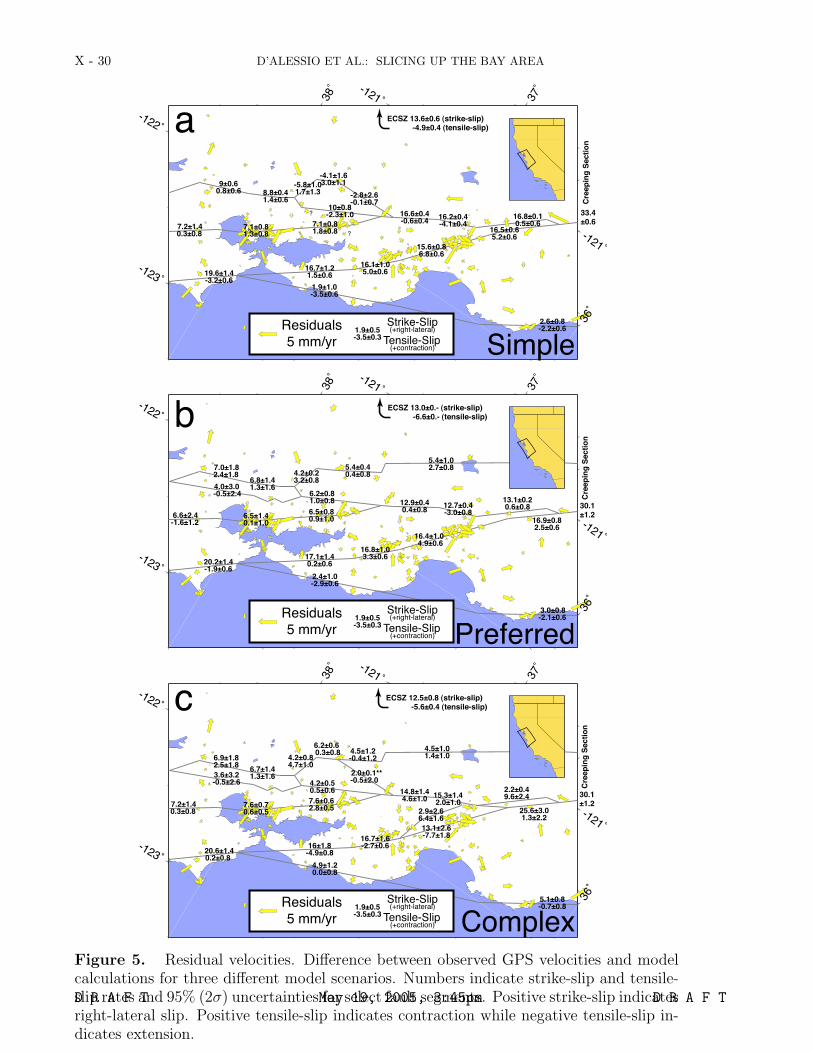
X - 30 D’ALESSIO ET AL.: SLICING UP THE BAY AREA
a
b
c
Simple
Preferred
Complex
??
?
Cre
ep
ing
Se
cti
on
Cre
ep
ing
Se
cti
on
Cre
ep
ing
Se
cti
on
Residuals
5 mm/yr
Strike-Slip(+right-lateral)
Tensile-Slip(+contraction)
Residuals
5 mm/yr
Strike-Slip(+right-lateral)
Tensile-Slip(+contraction)
Residuals
5 mm/yr
Strike-Slip(+right-lateral)
Tensile-Slip(+contraction)
Figure 5. Residual velocities. Difference between observed GPS velocities and modelcalculations for three different model scenarios. Numbers indicate strike-slip and tensile-slip rates and 95% (2σ) uncertainties for select fault segments. Positive strike-slip indicatesright-lateral slip. Positive tensile-slip indicates contraction while negative tensile-slip in-dicates extension.
D R A F T May 19, 2005, 3:45pm D R A F T
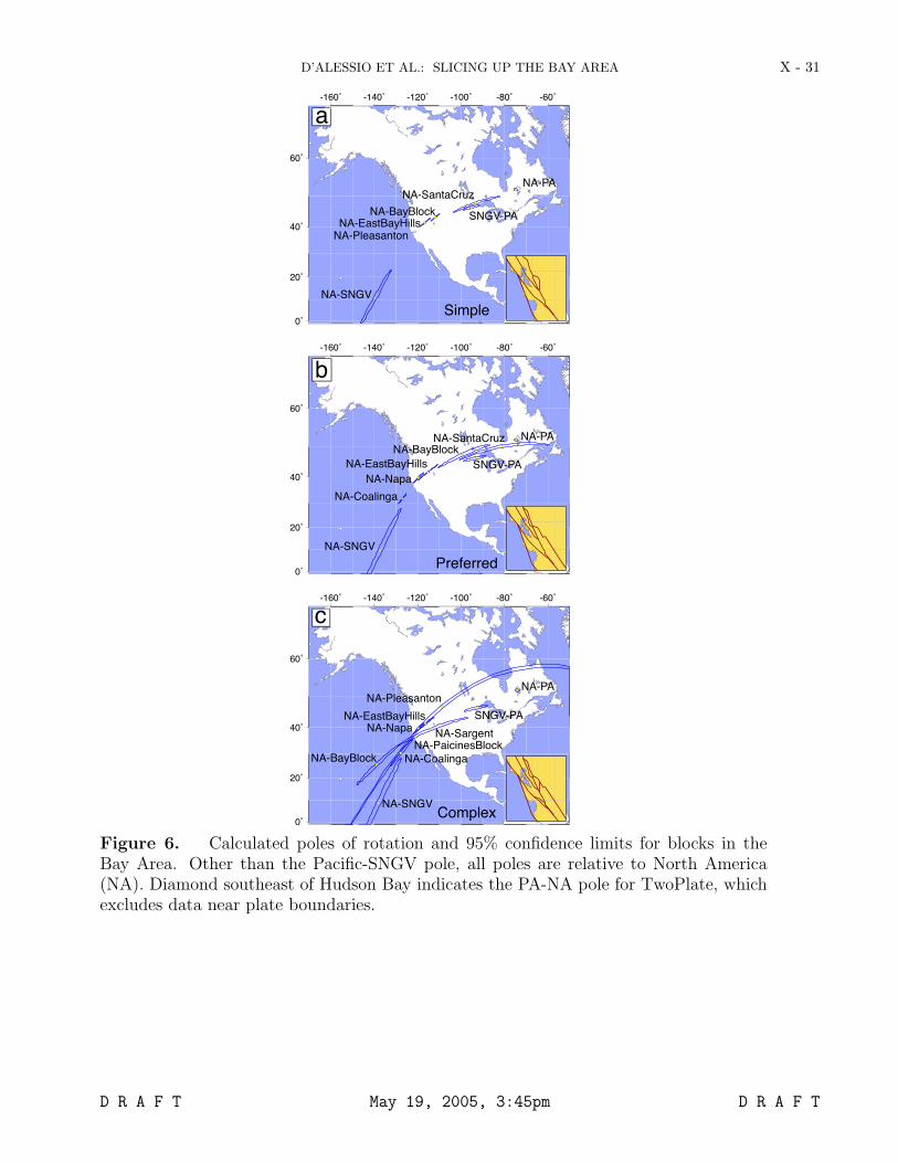
D’ALESSIO ET AL.: SLICING UP THE BAY AREA X - 31
SNGV-PA
NA-PA
NA-BayBlock
NA-EastBayHillsNA-Napa
NA-Pleasanton
NA-SNGV
NA-SargentNA-PaicinesBlock
NA-Coalinga
SNGV-PA
NA-PANA-BayBlock
NA-EastBayHills
NA-Napa
NA-SNGV
NA-Coalinga
NA-SantaCruz
SNGV-PA
NA-PA
NA-BayBlockNA-EastBayHillsNA-Pleasanton
NA-SNGV
NA-SantaCruz
b
Simple
Preferred
Complex
a
c
Figure 6. Calculated poles of rotation and 95% confidence limits for blocks in theBay Area. Other than the Pacific-SNGV pole, all poles are relative to North America(NA). Diamond southeast of Hudson Bay indicates the PA-NA pole for TwoPlate, whichexcludes data near plate boundaries.
D R A F T May 19, 2005, 3:45pm D R A F T
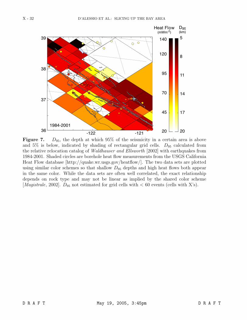
X - 32 D’ALESSIO ET AL.: SLICING UP THE BAY AREA
Figure 7. D95, the depth at which 95% of the seismicity in a certain area is aboveand 5% is below, indicated by shading of rectangular grid cells. D95 calculated fromthe relative relocation catalog of Waldhauser and Ellsworth [2002] with earthquakes from1984-2001. Shaded circles are borehole heat flow measurements from the USGS CaliforniaHeat Flow database [http://quake.wr.usgs.gov/heatflow/]. The two data sets are plottedusing similar color schemes so that shallow D95 depths and high heat flows both appearin the same color. While the data sets are often well correlated, the exact relationshipdepends on rock type and may not be linear as implied by the shared color scheme[Magistrale, 2002]. D95 not estimated for grid cells with < 60 events (cells with X’s).
D R A F T May 19, 2005, 3:45pm D R A F T
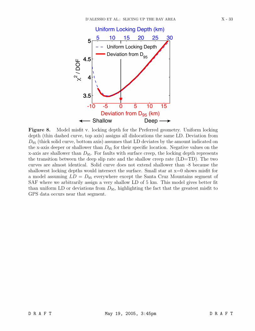
D’ALESSIO ET AL.: SLICING UP THE BAY AREA X - 33
3.5
4
4.5
5
3.5
4
4.5
5
Deviation from D95 (km)
5 10 15 20 25 30
3.5
4
4.5
5
2 /
DO
F
Uniform Locking Depth (km)
10-10 0-5 5 15
Shallow Deep
Uniform Locking Depth
Deviation from D95
Figure 8. Model misfit v. locking depth for the Preferred geometry. Uniform lockingdepth (thin dashed curve, top axis) assigns all dislocations the same LD. Deviation fromD95 (thick solid curve, bottom axis) assumes that LD deviates by the amount indicated onthe x-axis deeper or shallower than D95 for their specific location. Negative values on thex-axis are shallower than D95. For faults with surface creep, the locking depth representsthe transition between the deep slip rate and the shallow creep rate (LD=TD). The twocurves are almost identical. Solid curve does not extend shallower than -8 because theshallowest locking depths would intersect the surface. Small star at x=0 shows misfit fora model assuming LD = D95 everywhere except the Santa Cruz Mountains segment ofSAF where we arbitrarily assign a very shallow LD of 5 km. This model gives better fitthan uniform LD or deviations from D95, highlighting the fact that the greatest misfit toGPS data occurs near that segment.
D R A F T May 19, 2005, 3:45pm D R A F T
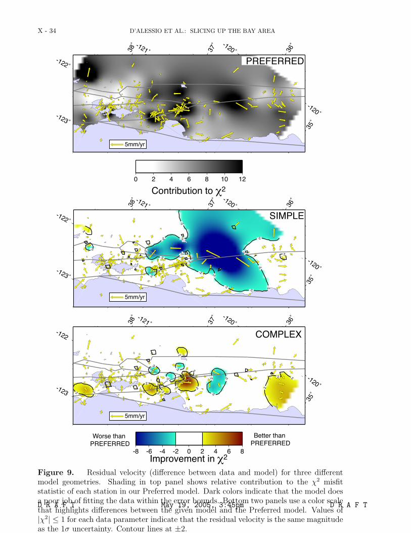
X - 34 D’ALESSIO ET AL.: SLICING UP THE BAY AREA
0 2 4 6 8 10 12
PREFERRED
SIMPLE
-8 -6 -4 -2 0 2 4 6 8
COMPLEX
-2
-2
-2
-2
-2
-2
-2
-2
-2
-2-2
-2
-2 -2
-2
-2
2
-2
-2
-2
-2
-2
2
2 2
22 2
2
2
2
2
2
2
-2
2
-2
Worse than
PREFERRED
Better than
PREFERRED
5mm/yr
5mm/yr
5mm/yr
Figure 9. Residual velocity (difference between data and model) for three differentmodel geometries. Shading in top panel shows relative contribution to the χ2 misfitstatistic of each station in our Preferred model. Dark colors indicate that the model doesa poor job of fitting the data within the error bounds. Bottom two panels use a color scalethat highlights differences between the given model and the Preferred model. Values of|χ2| ≤ 1 for each data parameter indicate that the residual velocity is the same magnitudeas the 1σ uncertainty. Contour lines at ±2.
D R A F T May 19, 2005, 3:45pm D R A F T
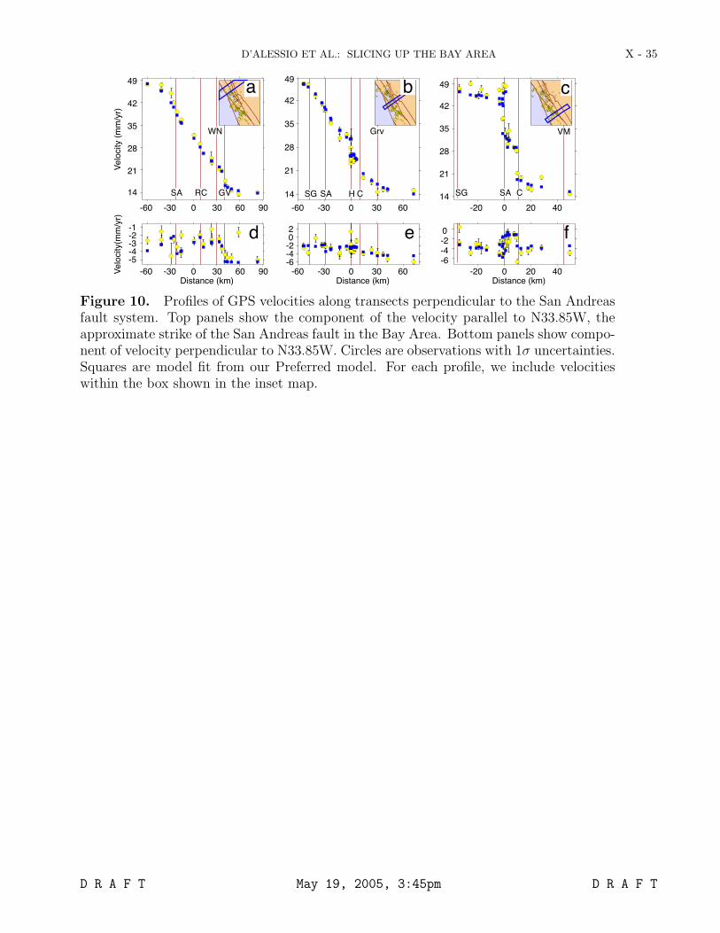
D’ALESSIO ET AL.: SLICING UP THE BAY AREA X - 35
14
21
28
35
42
49 49
Velo
city (
mm
/yr)
-60 -30 0 30 60 90
-5-4-3-2-1
Velo
city(m
m/y
r)
-60 -30 0 30 60 90Distance (km)
14
21
28
35
42
-60 -30 0 30 60
-6-4-202
-60 -30 0 30 60Distance (km)
14
21
28
35
42
49
-20 0 20 40
-6-4-20
-20 0 20 40Distance (km)
a b
d e
c
f
SA RC GV SA CSGSG SA H C
GrvWN VM
Figure 10. Profiles of GPS velocities along transects perpendicular to the San Andreasfault system. Top panels show the component of the velocity parallel to N33.85W, theapproximate strike of the San Andreas fault in the Bay Area. Bottom panels show compo-nent of velocity perpendicular to N33.85W. Circles are observations with 1σ uncertainties.Squares are model fit from our Preferred model. For each profile, we include velocitieswithin the box shown in the inset map.
D R A F T May 19, 2005, 3:45pm D R A F T
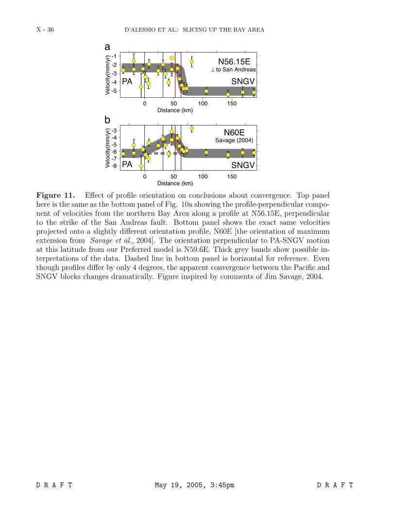
X - 36 D’ALESSIO ET AL.: SLICING UP THE BAY AREA
N60E
N56.15E to San Andreas
Savage (2004)
b
a
0 50 100 150Distance (km)
PA SNGV-8
-7
-6
-5
-4
-3
Velo
city(m
m/y
r)
-5
-4
-3
-2
-1
Velo
city(m
m/y
r)0 50 100 150
Distance (km)
PA SNGV
Figure 11. Effect of profile orientation on conclusions about convergence. Top panelhere is the same as the bottom panel of Fig. 10a showing the profile-perpendicular compo-nent of velocities from the northern Bay Area along a profile at N56.15E, perpendicularto the strike of the San Andreas fault. Bottom panel shows the exact same velocitiesprojected onto a slightly different orientation profile, N60E [the orientation of maximumextension from Savage et al., 2004]. The orientation perpendicular to PA-SNGV motionat this latitude from our Preferred model is N59.6E. Thick grey bands show possible in-terpretations of the data. Dashed line in bottom panel is horizontal for reference. Eventhough profiles differ by only 4 degrees, the apparent convergence between the Pacific andSNGV blocks changes dramatically. Figure inspired by comments of Jim Savage, 2004.
D R A F T May 19, 2005, 3:45pm D R A F T
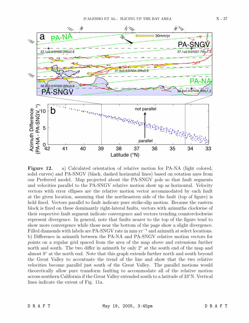
D’ALESSIO ET AL.: SLICING UP THE BAY AREA X - 37
?
30mm/yr
0
5
10
a
b
PA-NA
PA-NA
PA-SNGV
PA-SNGV
33343536373839404142
parallel
not parallel
Figure 12. a) Calculated orientation of relative motion for PA-NA (light colored,solid curves) and PA-SNGV (black, dashed horizontal lines) based on rotation axes fromour Preferred model. Map projected about the PA-SNGV pole so that fault segmentsand velocities parallel to the PA-SNGV relative motion show up as horizontal. Velocityvectors with error ellipses are the relative motion vector accommodated by each faultat the given location, assuming that the northeastern side of the fault (top of figure) isheld fixed. Vectors parallel to fault indicate pure strike-slip motion. Because the easternblock is fixed on these dominantly right-lateral faults, vectors with azimuths clockwise oftheir respective fault segment indicate convergence and vectors trending counterclockwiserepresent divergence. In general, note that faults nearer to the top of the figure tend toshow more convergence while those near the bottom of the page show a slight divergence.Filled diamonds with labels are PA-SNGV rate in mm·yr−1 and azimuth at select locations.b) Difference in azimuth between the PA-NA and PA-SNGV relative motion vectors forpoints on a regular grid spaced from the area of the map above and extensions furthernorth and south. The two differ in azimuth by only 2 at the south end of the map andalmost 8 at the north end. Note that this graph extends further north and south beyondthe Great Valley to accentuate the trend of the line and show that the two relativevelocities become parallel just south of the Great Valley. The parallel motions wouldtheoretically allow pure transform faulting to accommodate all of the relative motionacross southern California if the Great Valley extended south to a latitude of 33N. Verticallines indicate the extent of Fig. 11a.
D R A F T May 19, 2005, 3:45pm D R A F T
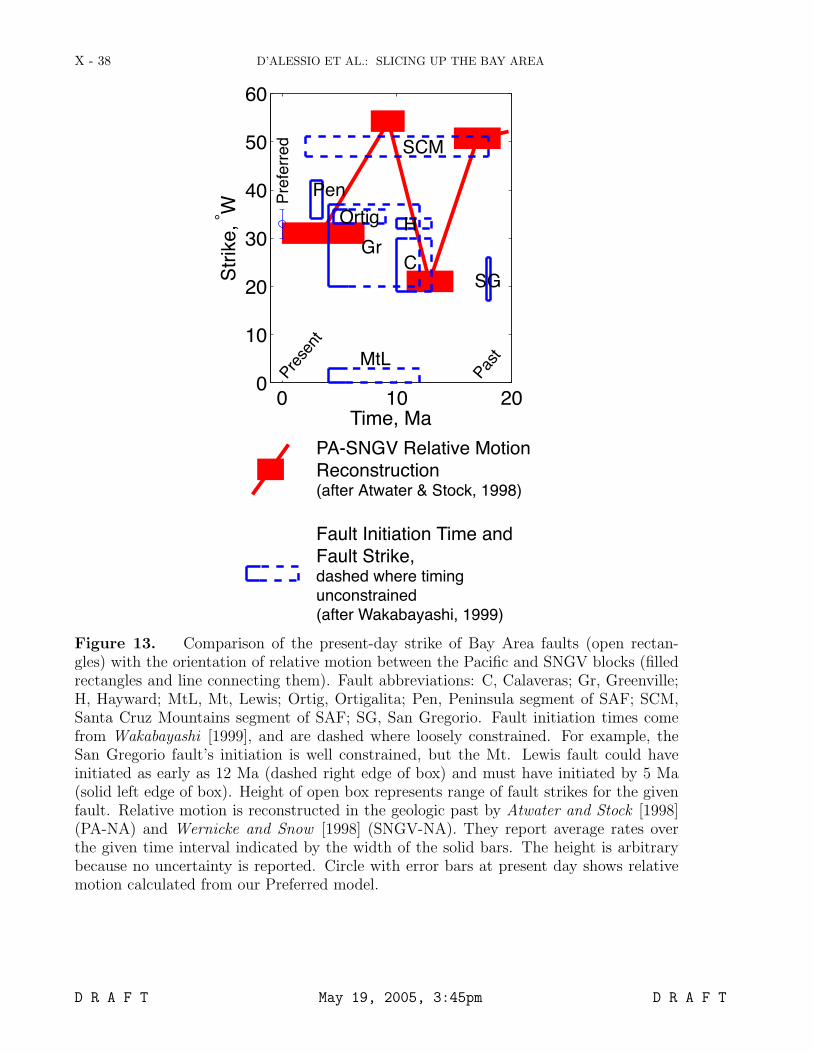
X - 38 D’ALESSIO ET AL.: SLICING UP THE BAY AREA
Pre
sent
Pas
t
0 10 200
10
20
30
40
50
60
Time, Ma
Str
ike,
W
SG
SCM
CGr
Ortig
Pen
MtL
H
PA-SNGV Relative Motion
Reconstruction(after Atwater & Stock, 1998)
Fault Initiation Time and
Fault Strike,dashed where timing
unconstrained
(after Wakabayashi, 1999)
Pre
ferr
ed
Figure 13. Comparison of the present-day strike of Bay Area faults (open rectan-gles) with the orientation of relative motion between the Pacific and SNGV blocks (filledrectangles and line connecting them). Fault abbreviations: C, Calaveras; Gr, Greenville;H, Hayward; MtL, Mt, Lewis; Ortig, Ortigalita; Pen, Peninsula segment of SAF; SCM,Santa Cruz Mountains segment of SAF; SG, San Gregorio. Fault initiation times comefrom Wakabayashi [1999], and are dashed where loosely constrained. For example, theSan Gregorio fault’s initiation is well constrained, but the Mt. Lewis fault could haveinitiated as early as 12 Ma (dashed right edge of box) and must have initiated by 5 Ma(solid left edge of box). Height of open box represents range of fault strikes for the givenfault. Relative motion is reconstructed in the geologic past by Atwater and Stock [1998](PA-NA) and Wernicke and Snow [1998] (SNGV-NA). They report average rates overthe given time interval indicated by the width of the solid bars. The height is arbitrarybecause no uncertainty is reported. Circle with error bars at present day shows relativemotion calculated from our Preferred model.
D R A F T May 19, 2005, 3:45pm D R A F T
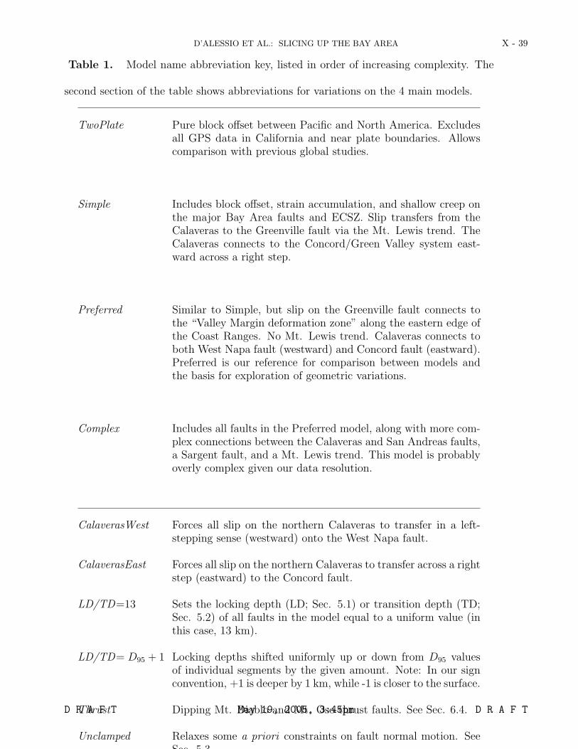
D’ALESSIO ET AL.: SLICING UP THE BAY AREA X - 39
Table 1. Model name abbreviation key, listed in order of increasing complexity. The
second section of the table shows abbreviations for variations on the 4 main models.
TwoPlate Pure block offset between Pacific and North America. Excludesall GPS data in California and near plate boundaries. Allowscomparison with previous global studies.
Simple Includes block offset, strain accumulation, and shallow creep onthe major Bay Area faults and ECSZ. Slip transfers from theCalaveras to the Greenville fault via the Mt. Lewis trend. TheCalaveras connects to the Concord/Green Valley system east-ward across a right step.
Preferred Similar to Simple, but slip on the Greenville fault connects tothe “Valley Margin deformation zone” along the eastern edge ofthe Coast Ranges. No Mt. Lewis trend. Calaveras connects toboth West Napa fault (westward) and Concord fault (eastward).Preferred is our reference for comparison between models andthe basis for exploration of geometric variations.
Complex Includes all faults in the Preferred model, along with more com-plex connections between the Calaveras and San Andreas faults,a Sargent fault, and a Mt. Lewis trend. This model is probablyoverly complex given our data resolution.
CalaverasWest Forces all slip on the northern Calaveras to transfer in a left-stepping sense (westward) onto the West Napa fault.
CalaverasEast Forces all slip on the northern Calaveras to transfer across a rightstep (eastward) to the Concord fault.
LD/TD=13 Sets the locking depth (LD; Sec. 5.1) or transition depth (TD;Sec. 5.2) of all faults in the model equal to a uniform value (inthis case, 13 km).
LD/TD= D95 + 1 Locking depths shifted uniformly up or down from D95 valuesof individual segments by the given amount. Note: In our signconvention, +1 is deeper by 1 km, while -1 is closer to the surface.
Thrust Dipping Mt. Diablo and Mt. Oso thrust faults. See Sec. 6.4.
Unclamped Relaxes some a priori constraints on fault normal motion. SeeSec. 5.3.
D R A F T May 19, 2005, 3:45pm D R A F T
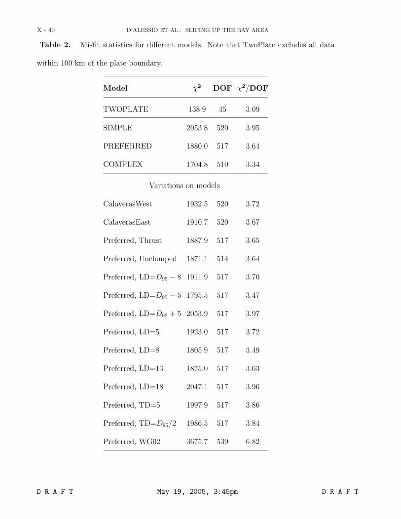
X - 40 D’ALESSIO ET AL.: SLICING UP THE BAY AREA
Table 2. Misfit statistics for different models. Note that TwoPlate excludes all data
within 100 km of the plate boundary.
Model χ2 DOF χ2/DOF
TWOPLATE 138.9 45 3.09
SIMPLE 2053.8 520 3.95
PREFERRED 1880.0 517 3.64
COMPLEX 1704.8 510 3.34
Variations on models
CalaverasWest 1932.5 520 3.72
CalaverasEast 1910.7 520 3.67
Preferred, Thrust 1887.9 517 3.65
Preferred, Unclamped 1871.1 514 3.64
Preferred, LD=D95 − 8 1911.9 517 3.70
Preferred, LD=D95 − 5 1795.5 517 3.47
Preferred, LD=D95 + 5 2053.9 517 3.97
Preferred, LD=5 1923.0 517 3.72
Preferred, LD=8 1805.9 517 3.49
Preferred, LD=13 1875.0 517 3.63
Preferred, LD=18 2047.1 517 3.96
Preferred, TD=5 1997.9 517 3.86
Preferred, TD=D95/2 1986.5 517 3.84
Preferred, WG02 3675.7 539 6.82
D R A F T May 19, 2005, 3:45pm D R A F T
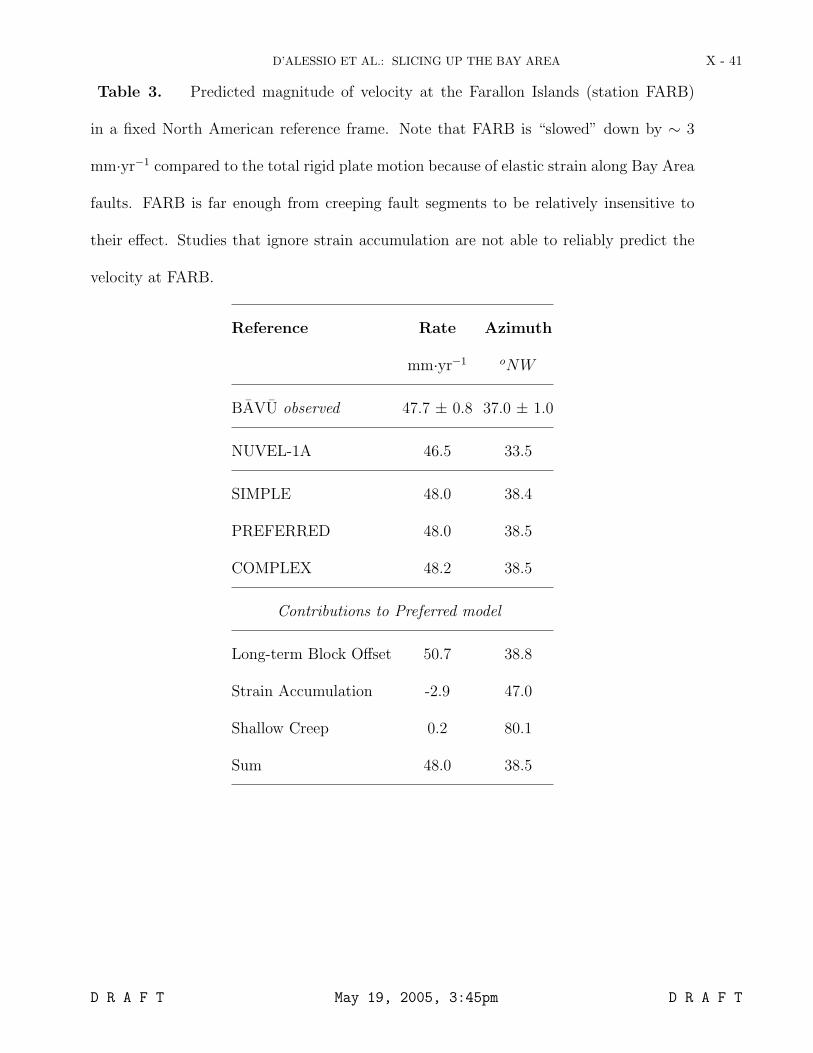
D’ALESSIO ET AL.: SLICING UP THE BAY AREA X - 41
Table 3. Predicted magnitude of velocity at the Farallon Islands (station FARB)
in a fixed North American reference frame. Note that FARB is “slowed” down by ∼ 3
mm·yr−1 compared to the total rigid plate motion because of elastic strain along Bay Area
faults. FARB is far enough from creeping fault segments to be relatively insensitive to
their effect. Studies that ignore strain accumulation are not able to reliably predict the
velocity at FARB.
Reference Rate Azimuth
mm·yr−1 oNW
BAVU observed 47.7 ± 0.8 37.0 ± 1.0
NUVEL-1A 46.5 33.5
SIMPLE 48.0 38.4
PREFERRED 48.0 38.5
COMPLEX 48.2 38.5
Contributions to Preferred model
Long-term Block Offset 50.7 38.8
Strain Accumulation -2.9 47.0
Shallow Creep 0.2 80.1
Sum 48.0 38.5
D R A F T May 19, 2005, 3:45pm D R A F T
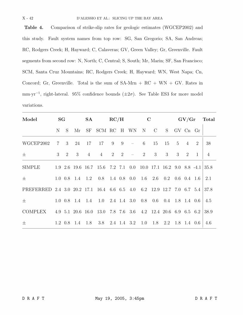
X - 42 D’ALESSIO ET AL.: SLICING UP THE BAY AREA
Table 4. Comparison of strike-slip rates for geologic estimates (WGCEP2002) and
this study. Fault system names from top row: SG, San Gregorio; SA, San Andreas;
RC, Rodgers Creek; H, Hayward; C, Calaveras; GV, Green Valley; Gr, Greenville. Fault
segments from second row: N, North; C, Central; S, South; Mr, Marin; SF, San Francisco;
SCM, Santa Cruz Mountains; RC, Rodgers Creek; H, Hayward; WN, West Napa; Cn,
Concord; Gr, Greenville. Total is the sum of SA-Mrn + RC + WN + GV. Rates in
mm·yr−1, right-lateral. 95% confidence bounds (±2σ). See Table ES3 for more model
variations.
Model SG SA RC/H C GV/Gr Total
N S Mr SF SCM RC H WN N C S GV Cn Gr
WGCEP2002 7 3 24 17 17 9 9 – 6 15 15 5 4 2 38
± 3 2 3 4 4 2 2 – 2 3 3 3 2 1 4
SIMPLE 1.9 2.6 19.6 16.7 15.6 7.2 7.1 0.0 10.0 17.1 16.2 9.0 8.8 -4.1 35.8
± 1.0 0.8 1.4 1.2 0.8 1.4 0.8 0.0 1.6 2.6 0.2 0.6 0.4 1.6 2.1
PREFERRED 2.4 3.0 20.2 17.1 16.4 6.6 6.5 4.0 6.2 12.9 12.7 7.0 6.7 5.4 37.8
± 1.0 0.8 1.4 1.4 1.0 2.4 1.4 3.0 0.8 0.6 0.4 1.8 1.4 0.6 4.5
COMPLEX 4.9 5.1 20.6 16.0 13.0 7.8 7.6 3.6 4.2 12.4 20.6 6.9 6.5 6.2 38.9
± 1.2 0.8 1.4 1.8 3.8 2.4 1.4 3.2 1.0 1.8 2.2 1.8 1.4 0.6 4.6
D R A F T May 19, 2005, 3:45pm D R A F T