skyline logging productivity under alternative harvesting
TRANSCRIPT

SKYLINE lOGGING PRODUCTIVITY UNDER
Al lERNA liVE HARVESTING PRESCRIPTIONS
AND lEVELS OF UTILIZA liON IN lARCH-FIR STANDS
Rulon B. Gardner
USDA Forest Service Research Paper INT-247
Intermountain Forest and Range Experiment Station U.S. Department of Agriculture, Forest Service
This file was created by scanning the printed publication.Errors identified by the software have been corrected;
however, some errors may remain.

~!
THE AUTHOR
RULON B. GARDNER was principal research engineer (now retired) , stationed at the Forestry Sciences Laboratory in Bozeman, Montana. He was involved in logging and road construction in National Forest Systems and Research for 25 years--the last 17 years in a research capacity.
RESEARCH SUMMARY
Little information is available to assess the economic and environmental feasibility of harvesting timber at more intensive levels of utilization in steep terrain. In this study in a larchfir stand, four levels of wood utilization, ranging from conventional saw log to almost total fiber recovery, were harvested using running skyline and live skyline yarding equipment. All four levels of utilization were applied under each of three silvicultural prescriptions--shelterwood, group selection, and clearcut harvesting.
The general objectives of the study were to determine the influence of intensive levels of wood utilization upon skyline system productivity under each silvicultural prescription, and to determine the important variables influencing rates of production.
The highest average production experienced, in total cubic feet of fiber removed, occurred in group selection cutting units for the running skyline yarding downhill in treatment 4--1,047 ft3/h (29.3 m3/h). The least productive logging occurred with the running skyline logging uphill in shelterwood cutting in treatment 3--353 ft 3/h (10.0 m3/h.
The most important variables influencing rate of production were yarding distance, lateral yarding distance to the skyline, and number of pieces per turn, in that order.

USDA Forest Service Research Paper INT-247
June 1980
SKYLINE LOGGING PRODUCTIVITY UNDER AL lERNA liVE
HARVESTING PRESCRIPTIONS AND LEVELS OF
UTILIZA liON IN LARCH-FIR STANDS
Ru I on B. Gardner
INTERMOUNTAIN FOREST AND RANGE EXPERIMENT STATION U.S. Department of Agriculture
Forest Service Ogden, Utah 84401
.... , ..

CONTENTS
INTRODUCTION .
OBJECTIVES .
EXPERIMENTAL HARVESTING UNITS ..
Logging Area and Blocks . .
PLANNING AND CONDUCTING HARVESTING .
Equipment . •
YARDERS. LOADERS. TRUCKS ..
Layout and Operation
Logging by Utilization Prescription
TIMBER VOLUMES LOGGED
HARVESTING PRODUCTIVITY
Felling and Bucking .
Yarding .
Loading .
Hauling .
FACTORS AFFECTING PRODUCTIVITY
ESTIMATING TURN TIME AND PRODUCTIVITY
SUMMARY AND CONCLUSIONS
PUBLICATIONS CITED
APPENDIX A--YARDER SPECIFICATIONS
Page 1
2
2
2
4
4
4 6 7
7
9
10
10
15
15
15
15
17
17
19
20
21
APPENDIX B--PRODUCTIVITY AND STATISTICAL ANALYSIS 23
The use of trade, firm, or corporation names in this publication is for the information and convenience of the reader. Such use does not constitute an official endorsement or approval by the u.s. Department of Agriculture of any product or service to the exclusion of others which may be suitable.

INTRODUCTION
The broad objective of the study on which this report is based was to evaluate skyline harvesting feasibility (economic and environmental) under the full array of silvicultural and utilization practices that could be used in managing a larch-fir timber stand.
Intensive wood utilization would reduce the waste of a valuable resource and extend an ever-shrinking wood fiber supply. Reductions in land available for growing timber because of urbanization and removal for other uses such as recreation, wildlife habitat, and wilderness, come at a time when demand for wood products continues to increase. Utilization of forest residues, estimated at 6 billion cubic feet (0.17 billion m3 )
annually, could increase the total fiber yield by as much as 50 percent on a national basis.
Intensive wood utilization can have pos1t1ve or negative environmental impacts, depending on the level of utilization, harvesting methods, and ecosystem response. Although some general information is available from past studies about responses-hydrology, flora, and fauna--the net results of applying increasing levels of timber utilization have not been adequately determined. Hence, a study was designed for the larch-fir type in Montana (fig. 1) to monitor biological-ecological responses to an array of alternative silvicultural and utilization timber harvesting prescriptions.
Figure I.--Experimental road and logging location.
"-CORAM EX PER I MENTAL FOREST Kalispelle ~
\ MONTANA Missoulae
KEY MAP
LEGEND:
EXPERIMENTAL ROAD •••••• ABBOT BAS IN ROAD --NO. 590. B ---
1

Because of the relatively steep slopes (45 to 60 percent) on the study area, cable yarding was appropriate. Past experience in the Rocky Mountain area has been largely with Idaho jammers or high-lead systems that require dense road networks because of limited skidding capabilities--300 to 500 ft (91 to 152 m) for jammer skidding and slightly more, 400 to 700 ft (122 to 213 m) for high-lead yarding.
For this experimental harvesting study, where one of the objectives was to reduce environmental impacts, it was decided to use a running skyline system to reduce road requirements. Road spacing was to be on the order of 1,500 to 2,000 ft (457 to 610 m); thus, the requirement for the basic system was a 1,000-foot (305 m) yarding capability uphill or downhill. Because of road width limitations and landing restrictions, the yarding equipment also had to be able to swing logs to the road. This report describes the logging methods, logging equipment, productivity, and factors affecting productivity.
OBJECTIVES
The specific objectives of the harvesting study were as follows:
1. Determine the influence of successively more intensive levels of wood utilization upon harvesting productivity for skyline systems operating under clearcut, shelterwood, and group selection silvicultural prescriptions.
2. Identify and quantify the stand and operation variables that significantly affect harvesting productivity.
3. Develop a statistical data base for estimating system yarding productivity, given some measure of the important variables describing the harvesting situation.
4. Develop, field test, and demonstrate harvesting practices and techniques that can improve the efficiency of running skyline systems, and thus enhance the opportunities for increased utilization.
In this report, the productivity experienced in each harvesting situation is presented and identified with the variables that influenced production.
The report further develops and illustrates procedures for estimating yarding turn time and associated productivity--a major cost determinant for the system.
EXPERIMENTAL HARVESTING UNITS
Logging Area and Blocks
Two blocks of each silvicultural prescription were laid out as shown in figure 1.
In each block, four levels of utilization were prescribed as shown in table 1. Treatment units run perpendicular to the slope.
The topography is generally steep (45 to 60 percent) and loggable only with cable equipment. To reduce hydrologic, esthetic, and biological impacts, logging equipment was needed that would reduce both the impacts from logging and attendant roads. The system also had to be portable and relatively easily rigged. The running skyline system was best for satisfying all of these requirements.
2

Table 1.--Logging area treatments and utilization prescriptions
Prescribed utilization
Conventional saw log
Close log utilization, trees 7 inches (17.8 em) d.b.h.+ (sawtimber trees)
Close log utilization, trees 5 inches (12. 7 em) d.b.h.+
Close fiber utilization, all trees
Material removed
Green and recent dead logs, to 5-1/2 inch (14 em) top; 1/3 or more sound
Green logs, to 3 inches x 8 ft (7.6 em x 2.4 m); dead and down logs, to 3 inches x 8 ft (7.6 em x 2.4 m), if sound enough to yard
Green logs, to 3 inches x 8 ft (7.6 em x 2.4 m); dead and down logs to 3 inches x 8 ft (7.6 em x 2.4 m), if sound enough to yard
Green 1-5 inches (2.5-12. 7 em) d.b.h. material tree length, in bundles; 2 green trees >5 inches (12. 7 em) d.b.h., tree length; dead and down, to 3 inches x 8 ft (7.6 em x 2.4 m), sound enough to yard
Postharvest treatment
Remaining understory slashed; broadcast burned
Understory retained; left as is
Remaining understory slashed; broadcast burned
Remaining understory slashed; left as is
Treatment designationl
1
2
3
4
1Treatment designation numbers used in this report are assigned in successive order of utilization intensity, 1 through 4. They do not correspond to the random treatment numbers assigned and used on the ground, which appear in various other reports based on this study site.
2Trees 1-5 inches (2.5-12. 7 em) d.b.h. cut and prebundled prior to logging activity on the site.
The upper part of blocks 11 and 12, all of 13, and the lower part of 21 were loggable from Abbott Basin Road 590-B, built in the 1950's (fig. 1). New access was needed for upper 21, 22, 23, and lower 11 and 12. Whenever it is desired to reduce road spacings in steep areas, it is usually efficient to gain elevation by switching back at favorable locations on the terrain and then log with a cable system with a fairly long reach. Figure 1 shows the new section of road that started from 590-B, near the upper part of block 11, and switched back on the gentle terrain of broad ridges to gain access above blocks 21, 22, and 23. A new short section of road was also built to access lower 11 and 12, as shown in figure 1. (A separate report by the author [Gardner 1978] describes the road portion of the study.)
3
'• :',

.. ·.··.·
YARDERS
PLANNING AND CONDUCTING HARVESTING
Equipment
The contractor selected a Skagit GT-3 (fig. 2) to meet the requirements for logging. Initial logging was done with the GT-3; later, two sides were logged simultaneously when a Link Belt 78 Log Mover (fig. 3) was put on the job. Both yarders had 1,000-foot (305 m) yarding capability. The Link Belt 78 was rigged as a live skyline using a gravity return carriage and, therefore, only able to log uphill. Figures 4 and 5 show how each system is rigged and operates (specifications for the yarder are in appendix A).
4
Figure 2.--Skagit GT-3 located at fan-shaped set below block 21 .
Figure 3.--Link Belt 78 Log Mover logging block 23.

Head spar
/
Carriage
~ Haulback Line
/
Figure 4.--Running skyline. Drums 1 and 2 on the yarder are interlocked for horsepower exchange during yarding operation, drum 3 operates the slack puller.
Head spar ~
Drum I-- Skyline drum Drum 2 --Main line drum
Figure 5.--Live skyline, gravity carriage. The skyline drum is powered so skyline tension can be varied during yarding operation.
5

' .. ·-···:··.
LOADERS
Three different types of loaders were used in situations that were normally hot logging operations (hot logging means skidding, loading, and hauling are going on simultaneously). For the first setting (block 21), which was downhill logging in a shelterwood cut, a jammer or heel boom loader was used (fig. 6). For all other loading, either a long boom (fig. 7) or a rubber-tired, front-end (fig. 8) loader was used. All loaders loaded both logs and currently unmerchantable material designated for removal under the more intensive utilization standards.
6
Figure 6.--Heel boom loading dump truck with residue from block 21.
Figure 7.--Long boom loader.

Figure 8.--Front-end loader working with Link Belt yarder keeping loading area clear on 14-foot (4.2 m) road without landings.
TRUCKS
Because of the large amount of currently nonmerchantable material that had to be removed to meet the previously discussed utilization standards, dump trucks were used for hauling this material. Conventional tractor-trailer units were used for the merchantable material.
Layout and Operation
The layout of blocks is shown in figure 1. Treatment units are numbered (1-4) and run perpendicular to the slope for clearcut and shelterwood blocks.
Planning logging sets and skyline roads is the key to successful operation of any cable logging system, particularly live or running skyline systems, which require deflection for suspension of the haulback line. In the generally uniform terrain (as seen by the contours in figure 1) of this logging chance, it was usually necessary to rig tail spar trees for deflection. The number and location of rigged tail spar trees are shown in table 2. Figure 9 shows a typical rigging, with nylon strap, block, and guylines. Only 14 of the 69 skyline sets did not require rigging to provide deflection.
7

I,:·.··,
Table 2.--Number of trees rigged when additional deflection was needed
Direction No. of Block yarded sets
11 up 7 (Selection cut) down 1
12 up 6 (Group selection down 4 cut)
13 up 5 (Clearcut)
21 up 5 (Selection cut) down 1
22 up 4 (Group selection cut)
23 up 7 (Clearcut)
Total 40
No. of No. roads
10
12
6
5
6
10
6
6
8
69
8
No. of of trees roads without
rigged rigged trees
9 1
5 7
6 0
1 4
6 0
9 1
6 0
5 1
8 0
55 14
Figure 9.--Typical tail spar rigging with nylon strap, block, and guylines.

For this study, the position of each skyline set was located cooperatively by the logger and research personnel. Potential sets were located on the topographic map and then investigated in the field. A field crew of two was trained to run levels from the set (road) to a suitable spar tree. A profile was then plotted to show the deflection needed to operate the set. A tree was rigged at the height necessary to provide the deflection. This step was done well ahead of the logging crew.
Topping of spar trees was deemed essential primarily for safety because of the risk of branches and dead tops shaking loose and dropping to the ground. Also, in the event of tail spar failure, the "radius of danger" would be less. Initially, topping was performed using about 60 sticks of dynamite with a Primacord belt wrapped around an 18- to 24-inch (45. 7 to 56.9 em) diameter tree. An improved technique was developed that utilized six or seven pouches of a liquid/powder mixture with holes through each pouch using Primacord like a string of beads. The belt of explosives was installed at the point of topping by a rigger who would climb the tree with conventional pole climbing apparatus and lower a rope to raise the belt of explosives. Then a length of Primacord sufficient to reach the ground was tied to the belt. Finally a detonating cap and a length of fuse were attached to the end of the Primacord that reached the ground. The fuse was of sufficient length to allow all personnel to walk several hundred feet from the impending blast. Before igniting the fuse, the yarder operator was contacted by radio, and he activated his whistle-signaling device to warn everyone in the area of the blast.
The explosion caused a relatively clean, horizontal severance, with a zone of crushing and ring separation extending no greater than about 12 inches (30.5 em) from the cut.
All skyline roads were held to a maximum width of 10 ft (3.05 m) in the shelterwood blocks, and in leave strips between group selection blocks, to reduce visual impacts.
Logging for the most part was conducted as a hot logging operation. Landings were usually not available, with the exception of the downhill yarding in blocks 11, 12, and 21. Downhill yarding from blocks 11 and 12 was to open, near-level areas seen from the contours in figure 1. A stretch of wide road between the yarder and block 21 was used as a landing (fig. 3) for downhill yarding in that block. A typical set yarding to the road is seen in figure 4. This photograph illustrates why the yarders were required to have swing capability so they could land the logs on the road.
The yarding crews consisted of the operator, two choker setters, a knot bumperchaser, and a side foreman, who supervised both yarding crews. The loading and hauling operations were required to keep logs clear of the yarder. Merchantable material and unmerchantable were separated at the landing by the loaders or loaded directly to the truck, depending on the situation at the yarder and availability of the trucks. The usual situation was trucks waiting for loads.
logging by Utilization Prescription
Recall that the primary purpose of the study was to determine the economic and environmental impacts of different levels of utilization under alternative silvicultura1 practices. Previous studies had indicated that it may be possible to utilize sawtimber trees down to 3-inch (7.6 em) diameters in lengths of at least 8 feet (2.4 m); i.e., treatment 3. Treatments 4 and 2 are respectively more and less intensive than 3 to adequately identify feasibility limits.
9

Conventional sawlog (1).--In this treatment, the logs were yarded in a conventional manner with the limbs and top removed. The slash was disposed of by broadcast burning.
Close log utilization (2, 3).--All of the material was yarded to meet the utilization prescriptions as defined in table 1.
Close fiber utilization (4).--In treatment 4, trees were yarded as whole trees (or as nearly so as possible) and the merchantable logs removed in the conventional manner. Lirnbing and topping was accomplished on the landing.
One operation in treatment 4 was unique to this study. The understory trees designated for removal (1 to 5 inches [2.54 to 12.7 ern]), were cut and bundled by research crews prior to any logging activity, and subsequently yarded by the contractor. Rope was used to make a bundle the size a choker could handle--about 3 ft (0.9 rn) in diameter and tree length long. A choker was put around the bundle for yarding. Handling the understory material in this manner was the only practical way to achieve intensive fiber recovery because it is not economically feasible to yard very small pieces individually.
In systems other than clearcutting, it can be difficult to yard material laterally. Before logging began, it was thought that yarding downhill in selectively cut blocks could cause serious problems because the load would have to be turned downhill in a fairly narrow corridor when it reached the skyline road. However, this did not prove to be as difficult as anticipated.
TIMBER VOLUMES LOGGED Preharvest inventory of all material was at a more intensive level than for ordinary
sales because a good estimate of the total biomass was desired for estimating potential removals. All harvested and removed material was also measured at the landing except solid volumes for bundled material from treatment 4 that were estimated. Table 3 shows inventoried and removed volumes by block and treatment. Removals in treatment 4 for blocks 21 and 22 exceed inventoried estimates. Since removal measurements represent a 100 percent sample, it is believed they are more accurate. Inventoried merchantable volumes per acre in treatments varied from approximately 2,050 ft 3/acre (140 rn 3/ha) (8,660 bd.ft./acre) to over 6,000 ft3/acre (420 rn3/ha) (25,980 bd.ft./acre). From a total volume of fiber removed of 405,879 ft3 (11 494 rn3), 298,455 ft 3 (8 452 rn 3) (1,292,310 bd.ft.) was merchantable or 74 percent.
HARVESTING PRODUCTIVITY The differences in timber composition, size, and density among blocks allows for
productivity comparisons only between treatments within blocks. Therefore, conclusions about productivity differences between silvicultural prescriptions should not be attempted. Also, the differences in landing conditions along with the above tend to confound differences between uphill and downhill yarding production.
10

Table 3.--Preharvest and removed volumes (ft 3)
Volumes Percent Block/treatment Acres Preharvest Removed removal
11-1 14.9 98,027 21,495 21.9 -2 6.2 37,324 17,368 47.3 -3 6.7 47,603 17,545 36.9 -4 7.3 48,854 48,354 99.0
Subtotal 35.1 231,808 104,762 45.2
12-1 2.3 14,823 6,537 44.1 -2 1.7 16,232 8,668 53.4 -3 1.7 14,341 10,407 72.6 -4 1.9 18,344 16,244 88.5
Subtotal 7.6 63,740 41,856 65.7
13-1 3.8 26,325 14,668 55.7 -2 3.2 24,333 18,481 76.0 -3 2.9 26,248 9,676 36.9 -4 3. 7 26,366 14,975 56.1
Subtotal 13.6 103,272 57,800 56.0
21-1 4.8 31,834 12,539 39.4 -2 4.6 25,056 19,554 78.0 -3 6.7 42,572 30,946 72.7 -4 5.4 26,881 29,572 110.0
Subtotal 21.5 126,343 92,611 73.3
22-1 1.3 14,404 7,710 53.5 -2 1.5 14,493 8,231 56.8 -3 1.6 17,029 12,564 73.8 -4 1.6 11,562 11,818 102.2
Subtotal 6.0 57,488 40,323 70.1
23-1 3.4 34,476 11,343 32.9 -2 3.4 25,711 8,721 33.9 -3 5.1 39,414 26,738 54.1 -4 4.7 32,002 21,740 67.9
Subtotal 16.6 131,603 68,542 52.1 Total 100.4 714,254 405,879 56.8
Tables 4, 5, and 6 summarize data related to each silvicultural system, including acreage, volumes, layout and equipment, and average yarding production by equipment type, treatment, and direction of yarding. The mean, standard deviation, and standard error by block and direction of yarding for pieces per turn, turns per hour, and pieces per hour are summarized in appendix B (table 9).
Productivity data were derived from time and motion studies. These studies extended over the entire duration of the logging, covering over 7,200 turns made by the running and live skyline systems.
11
I ,,'<- .... ~

Table 4.--Skyline yarding summary--shelterwood units
LOGGING UNITS
Block Block Number Average piece number size Total volume pieces size
Acres ha Ft 3 m3 Ft 3 m3
11 35.1 14.2 104,762 2 967 7,471 14.02 0.397 21 21.5 8. 74 92,611 2 623 6,338 14.61 .414
YARDING LAYOUT
Block Number skyline roads Yarding distance number Uphill Downhill Average Range
Ft m Ft m
11 10 12 508 155 0-1,050 0-320 21 10 6 557 170 25-1,150 8-350
EQUIPMENT
21 Yarding - Skagit GT-3 rigged as running skyline, yarding uphill and downhill Loading - Both long boom and front end loader used at times Hauling- 6.0 M bd.ft. truck and trailers for logs, and 10-yard dumps for
residues
11 Yarding Skagit GT-3 rigged as running skyline, yarding uphill and. downhill Link Belt 78 Log Mover rigged as a live skyline, yarding uphill
Loading - Same as Block 21 Hauling - Same as Block 21
Treatment
Conventional saw log (1) Close log, trees 7"+ (2) Close log, trees 5"+ (3) Close fiber (4)
Conventional saw log (1) Close log, trees 7"+ (2) Close log, trees 5"+ (3) Close fiber (4)
Close log, trees 7"+ (2) Close fiber (4)
AVERAGE PRODUCTION PER HOUR 1
System
Running skyline, uphill yarding
Running skyline, downhill yarding
Live skyline, uphill yarding
Total volume Ft m
497 13.6 358 10.1 353 10.1 568 16.1
644 18.2 561 15.9 615 17.4 813 23.0
321 9.1 747 21.2
1Production per hour includes foreign element delay time occurring within a turn cycle, but not nonproductive hours for rest breaks, repairs, rerigging, etc. Foreign element delays are those caused by machines, manpower, materials, or environmental factors.
12

Table 5.--Skyline yarding summary--group selection units
LOGGING UNITS
Block Block Number Average piece number size Total volume Eieces size
Acres ha Ft 3 m3 Ft 3 m3
12 7.60 3. 04 41,856 1 185 2,670 15.63 0.443 22 6.0 2.40 40,323 1 142 2,585 15.60 .442
YARDING LAYOUT
Block Number skyline roads Yarding distance number U£hill Downhill Average Range
Ft m Ft m
12 6 5 322 98 50-760 15-232 22 6 0 524 160 0-1,250 0-381
EQUIPMENT
12 Yarding - Skagit GT-3 rigged as running skyline and yarding downhill only Link Belt 78 Log Mover rigged as a live skyline and yarding uphill
Loading - Both long boom and front end loader used at times Hauling - 6.0 M bd.ft. truck and trailers for logs, and 10 yard dumps for
residues
22 Yarding Skagit GT-3 rigged as running skyline and yarding uphill only Link Belt 78 Log Mover rigged as a live skyline and yarding uphill
Loading - Same as Block 12 Hauling - Same as Block 12
AVERAGE PRODUCTION PER HOUR 1
Treatment System Total volume Ft m
Conventional saw log (1) Running skyline, uphill 500 14.2 Close log, trees 7"+ (2) yarding 590 16.7 Close log, trees 5"+ (3) 590 16.7 Close fiber (4) 490 13.9
Conventional saw log (1) Running skyline, downhill 826 23.4 Close log, trees 7"+ (2) yarding 815 23.1 Close log, trees 5"+ (3) 815 23.1 Close fiber (4) 1' 04 7 29.7
Conventional saw log (1) Live skyline, uphill yarding 511 14.5 Close log, trees 7"+ (2) 469 13.3 Close log, trees 5"+ (3) 605 17.1 Close fiber (4) 816 23.1
lsee table 4 footnote.
13
.. , '

Block number
13 23
Block number
13 23
13
23
Table 6.--Skyline yarding summary--clearcut units
LOGGING UNITS
Block Number Average piece size Total volume pieces size
Acres ha Ft 3 m3 Ft3 m3
13.60 5.44 57,800 1 637 3,906 14.80 0.419 16.6 6.64 68,542 1 941 5,201 13.18 .373
YARDING LAYOUT
Number skyline roads Yarding distance Uphill Downhill Average Range
Ft m Ft m
6 0 478 146 50-900 15-274 8 0 488 149 0-950 0-290
EQUIPMENT
Yarding Skagit GT-3 rigged as a running skyline and yarding uphill only Loading Both long boom and front end loader used at times Hauling - 6.0 M bd.ft. truck and trailers for logs and 10 yard dumps for
residues
Yarding - Link Belt 78 Log Mover rigged as a live skyline and yarding uphill Loading - Same as Block 13 Hauling - Same as Block 13
AVERAGE PRODUCTION PER HOUR1
Treatment System Total volume
Conventional saw log (1) Close log, trees 7"+ (2) Close log, trees 5"+ (3) Close fiber (4)
Conventional saw log (1) Close log, trees 7"+ (2) Close log, trees 5"+ (3) Close fiber ( 4)
lsee table 4 footnote,
Running skyline, uphill yarding
Live skyline, uphill yarding
14
Ft
989 622 850 583
930 503 632 595
m
28.0 17.6 24.1 16.5
26.4 14.2 17.9 16.8

Felling and Bucking Time and motion studies did not include felling and bucking. Production and cost
were estimated for the sale, using Northern Region timber sale appraisal guides. The base cost adjusted for average d.b.h., trees/acre, slope, and tree defect was $11.86/M bd.ft. ($2.62/m 3) (1974). This cost was assumed to be applicable to clearcut units under conventional saw log specification, or treatment 1. It was adjusted for the requirements of the other treatments as follows:
+32.5 percent for cutting 5- to 7-inch (12.7 to 17.8 em) d.b.h. in treatment 3. +50.0 percent to avoid damaging residual in shelterwood units. +50.0 percent to avoid damage to adjoining stands near group selection units. +10.0 percent for limbing to 3-inch (7.6 em) top in treatments 2 and 3.
It was assumed that production, and therefore cost, would be equal to Regional averages, with the above added for special treatment requirements.
Comparing observed sawyer production with estimated production shows a slight overestimation in some treatments and underestimation in others, with similar averages: 0.79 M bd.ft./h (3.58 m3/h) observed production rate vs. 0.87 M bd.ft./h (3.94 m3/h) estimated production rate (table 10 in appendix B).
Yarding The greatest productivity for total solid volumes was from group selection units
using a running skyline logging downhill--1,047 ft 3 (29.6 m3) per hour in treatment 4. The least productive logging was in running skyline units logging uphill in shelterwood blocks--productivity was 353 ft 3 (10.0 m3) in treatment 3. Factors affecting productivity are discussed in detail in the next section.
Nonproductive time--yarding.--The percentage of total yarding time actually spent yarding was estimated for each block from data recorded by research personnel (table 11, appendix B). These times could be expected to vary between organizations.
Loading Time and motion studies were not made for the loading operation. However, a record
was kept of the number and type of trucks loaded each day. In table 12 (appendix B) the mean, standard deviation, and standard error for trucks loaded per day are shown for each operation.
Waiting and loading times for log and dump trucks were recorded for a sample of logging sets as shown in table 7.
Hauling Hauling distance for the dump trucks was approximately 7.5 miles (12.1 km) to the
disposal area--an average of 1 mile (1.6 km) on the new road and 6.5 miles (10.4 km) of single-lane, unsurfaced road with turnouts (No. 590). Hauling distance for the logs to the Columbia Falls, Mont., mill consisted of approximately 1 mile (1.6 km) on the new road, 5.8 miles (9.3 km) of single-lane, unsurfaced road with turnouts, 1.5 miles (2.4 km) of lane and one-half [20ft (6.1 m)] gravel surfaced, and 10 miles (16.1 km) of paved, double-lane (U.S. No. 2) for a total of 17.3 miles (27.8 km). A tabulation of transport mileages for logs and residue and estimated average speed and hours of travel one way is shown in table 8.
15

Table 7.--Waiting and loading times for log and dump trucks (in hours)
Log trucks Unmerchantable trucks Statistic Waiting Loading Waiting Loading
n 32 32 32 32
X 2.43 1. 89 1. OS 0.86
Sx 1. 56 1.18 1. 31 1. 24
n number of observations.
x = mean waiting or loading time.
Sx standard error of the mean.
Table B.--Transport distances and times for merchantable and residue material
Road section Distance Average sEeed Miles km Mi/h km/h
Residue
New section 590B 1.0 1.6 15 24.1
Old section 590B 6.5 10.4 17 27.4
Total
Logs
New section 590B 1.0 1.6 15 24.1
Old section 590B 5.8 9.3 17 27.4
Country road 1.5 2.4 24 38.6
u.s. No. 2 10.0 6.1 so 80.4
Total
Nonproductive time is not included.
16
Hours
0.067
.382
0.449
.067
.341
.341
.200
0.670

FACTORS AFFECTING PRODUCTIVITY In this study, the principal variables influencing yarding were distance, lateral
distance, slope, volume, number of logs, and weight in various combinations, depending on the equipment and silvicultural prescription.
The principal variables influencing the production of logging systems and equipment are fairly well known from studies conducted over the years. However, the relative influence of some variables is still being debated by researchers. Therefore, all of the variables thought to be potentially significant for influencing production were recorded using a standardized methodology developed over the past several years by Intermountain Station's Engineering Research Work Unit at Bozeman, Mont.
The final equations for logging production were selected on the basis of the simultaneous consideration of the following criteria discussed in more detail by Gibson (1975).
1. R2 or percent of variation explained by the equation. 2. F-ratio for significance of the regression. 3. Standard error of the independent variable (expressed as a percentage of the
mean). 4. Analysis of residual plots. 5. Subjective consideration of information available to those who may use the
equations for predicting production.
The principal variables retained for each equation as a result of the above criteria are shown in table 13 (appendix B). Also table 14 (appendix B) shows the significance of the variables. Distance was the major variable influencing production in every case. Lateral distance appears in every equation except for the live skyline in shelterwood units. All equations are for the conventional logging utilization treatments (1).
ESTIMATING TURN TIME AND PRODUCTIVITY Harvesting productivity in general, and for the Coram sale in particular, was
discussed under harvesting productivity (tables 4, 5, and 6). These statistics are useful for comparing production for different utilization standards, and equipment types used on the sale. They show what could be expected at other locations with conditions similar to those at Coram, but what about other areas and situations?
Regression equations (appendix B, table 13) can be used to estimate production when information is available about the independent variables. Most of this information is available whenever a sale is prepared or can be derived from timber surveys and topographic maps.
To facilitate the use of the regression equations and foreign element delay times derived from the study, tables 15 through 23 in appendix B were prepared. They can be used to estimate turn time computed from each equation in table 13, appendix B.
To illustrate how productivity can be estimated, the following examples are presented.
17

Computation of Turn Time and Productivity for Assumed Yarding Conditions (all tables used are in appendix B)
Case 1: Running skyline, shelterwood cut, uphill yarding --Average yarding distance--500 feet (152 m) --Average lateral yarding distance--60 feet (18. 3 --Average number of logs--4.0 --Average weight of load--2,800 lb (1,270 kg) --Average piece size--14 ft 3 (0. 33 m3)
Estimating Turn Time (T.T.)
from table 15:
Matrix A, factor = 5.87 (extrapolated) Matrix B, factor= 1.027 T.T. 5.87 x 1.027 = 6.03 min
from table 22: Percent foreign element 14.4
T.T. = 6.03 X 1.144 = 6.72
Estimating Productivity
Turn time = 6. 72
from table 23:
4.0 logs, 14 ft 3 (0.33 m3) piece size V = 501 ft 3/h (14.2 m3/h) (extrapolated)
(These are productive hours for all estimates.)
Case 2: Live skyline, clearcut, uphill yarding --Average yarding distance--400 feet (122 m)
m)
--Average lateral yarding distance--90 feet (27.4 m) --Average number of logs--5.0 --Average slope--60 percent --Average piece size--12 ft3 (0.29 m3)
Estimating Turn Time (T.T.)
from table 21:
Matrix A, factor= 10.16 (extrapolated) Matrix B, factor= 0.612 T.T. 10.16 x 0.612 = 6.22
from table 22: Percent foreign element 10.8
T.T. = 6.22 x 1.108 = 6.89
Estimating Productivity
Turn Time= 6.89
from table 23:
5. 0 logs, 12 ft 3 (0. 29 m3) piece size V = 512 ft 3/hr (14.5 m3/hr) (extrapolated)
(These are productive hours for all estimates.)
18

, ..
SUMMARY AND CONCLUSIONS For shelterwood and group selection units, the cubic foot volume of material removed
per hour was greatest in treatment 4, as would probably have been expected. However, cubic foot volume removed per hour in clearcut units was greatest in treatment 1 (conventional logging). Production per hour was generally greater for all treatments in clearcut units. This may have been due to greater ease of lateral skidding.
The important measured variables influencing turn cycles, and therefore production, were (1) distance, (2) lateral distance, (3) slope, (4) number of logs, (5) volume, and (6) weight. In table 14 (appendix B), the relative importance of these variables for each harvesting situation is shown by their contribution to the correlation coefficient (R2 ). Distance was the most important variable in every case, and lateral distance appears in every equation. Number of logs appears in every equation except the running skyline yarding uphill in a shelterwood cut. If information is available for these three variables, a reasonably good estimate of production is possible.
The room to maneuver yarders, trucks, and loaders on this sale was rather restricted because of the 14-foot (4.3 m), single-lane road, few turnouts, and no planned landings. In fact, landing construction was prohibited. However, turnouts could be used effectively as could the relatively flat areas below blocks 11 and 12. These landing areas in blocks 11 and 12 were undoubtedly partly responsible for the greater production experienced from downhill yarding in these blocks.
19

PUBLICATIONS CITED Gardner, Rulon B.
1978. Cost, performance, and esthetic impacts of an experimental forest road in Montana. USDA For. Serv. Res. Pap. INT-203, 28 p. Intermt. For. and Range Exp. Stn. , Ogden, Utah.
Gibson, David F. 1975. Evaluating skyline harvesting productivity. Winter Meet., Am. Soc. Agr. Eng.
Proc. [Chicago, Ill.], 38 p.
20

APPENDIX A--YARDER SPECIFICATIONS
GENERAL YARDER SPECIFICATIONS
Skagit GT-3
Dimensions: Boom Height- 38 1 6" (11.7 m) Working Height - 44 1 (13.4 m) Overall Width - 12 1 6" (3.8 m) Ground Clearance- 1 1 4" (0.4 m)
Drum Capacity:
Mains - 1,700 1 (518 m) - 5/8" (1. 6 em) 1,100 1 (335 m) - 3/4" (1. 9 em)
Haul back - 2,400 1 (732 m) - 3/4" (1. 9 em) 2,600 1 (792 m) - 3/8" (1. 0 em)
dia. dia.
dia. dia.
cable cable
cable cable
Guyline - 109 1 (33.2 m) - 1" (2.54 em) dia. cable
Power Unit - Cummings NH 220 with Allison Torque Converter
Shipping Weight - 95,040 lb (43,110 kg)
Dimensions:
Drum Capacity:
Link Belt HC-78B
Boom Height - 35 1 0" (1 0. 7 m) Working Height - 41 1 5" (12. 6 m) Overall Width- 9 1 0" (2.7 m) Minimum Ground Clearance - 0 1 10" (2.1 em)
Sky 1 in e - 1 , 1 0 0 1 ( 3 3 5 m) - 5 I 8" ( 1. 6 em) d i a . cab 1 e
Mainline - 1,300 1 (396m) - 1/2" (1.3 em) dia. cable
Power Unit - General Motors 6V-53
Shipping Weight - 68,775 lb (29,958 kg)
21


APPENDIX B--PRODUCTIVITY AND STATISTICAL ANALYSIS
Table 9.--Mean, standard deviation, and standard error for pieces per turn, turns per hour, and pieces per hour
Pieces/turn Turns/hour Pieces/hour Blockl/; ---~2~~----~--~----------------------~~--------------------------~----------
x- Sx Sx x Sx Sx x Sx Sx
210 (S) llD(S)
21U(S) llU (S)
22U(GS) l2D(GS)
l3U(C)
ALL
22(GS) 12(GS)
11 (S)
23 (C)
ALL
Yo
2/ ~
SKAGIT
2.39 0.63 0.18 10.64 2.96 0.86 25.58 10.30 4.37 .59 .13 10.89 2.90 .63 47.09 11.17
3.63 .56 .16 8.82 3.25 .60 35.42 13.15 3.89 .55 .16 9.13 2.40 .62 .)4. 37 11.67
4.74 . 74 . 21 6. 72 2.63 .73 31.79 13.22 5.16 .84 .25 ll. 23 2.17 .65 57.98 14.63
4.4 7 .61 .14 9.73 l. 65 . 39 42.40 7.49
4.14 l. 02 10.12 6.84 39. 14 14.48
LINK BELT
4.60 l. 52 . 76 7.82 2. 27 l. 36 38.40 22.35 4.60 .44 .17 9.39 l. 24 .44 43.46 6.61
4.96 .65 .19 7.74 l. 97 .57 36.60 10.65
4.89 .96 .19 8. 43 2. 13 .43 45.71 19.44
4.84 .87 8.19 2.04 38.54 13.96
downhill yarding, U = uphill yarding, S = shelterwood, GS = group selection, clearcut. mean, Sx = standard deviation, Sx = standard error of the mean.
Table 10.--Falling statistics
Treatment and Observed Estimated production si1vicultural cut production rate rate based on cost
h/M bd.ft. (h/m 3) h/M bd.ft. (hjm 3 )
ll l - cc 0.58 (0. 13) 0.58 (0.13) - GS .69 (0.15) .87 (0.19) - sw .93 (0.21) .87 (0.19)
4 - cc .59 (0. 13) .77 (O. l 7) 4 - GS .60 (0. 13) l. 06 co. 23) 4 - sw l. 01 (0.22) l. 06 (0. 23) 3 - cc .68 (0.15) .82 (0. 18) 3 - GS .74 (0.16) l. 11 (0.24) 3 - sw 1.15 (0.25) l. ll (0.24) 2 - cc .72 (0. 16) .64 (0. 14) 2 - GS .81 (0. 18) .93 (0. 21) 2 - sw 1. 21 (0.27) .93 (0. 21)
Average .79 ( 0. l 7) . 87 (0. 19)
y Basis for estimates.
23
2.97 2.44
2.44 3.01
3.67 4.41
1.77
11. 17 2.70
3.08
5.39

Block
11 12 13 21 22 23
Table 11.--Estimates of productive hours
Percentage of total yarding time actually spent yarding
0.66 .70 .79 .67 .59 .65
Average 0.67
Table 12.--Loading statistics for each operation
Loader
Long boom Front end
Truck
Logs-trailer Residue-dump
Loader
Long boom Front end
Truck
Logs-trailer Residue-dump
SKAGIT
Trucks loaded per day
X
5.00 3.20
Sx
2.85 1. 57
Trucks loaded per day by class
-X
2.35 3.19
LINK BELT
Sx
1. 56 2.29
Trucks loaded per day
-X
3.79 4.44
Sx
1. 44 2.50
Trucks loaded per day by class
-X
2.21 3.23
24
Sx
1.10 1. 78
sx
0.49 .40
sx
0.18 .31
sx
0.33 .59
sx
0.21 .33
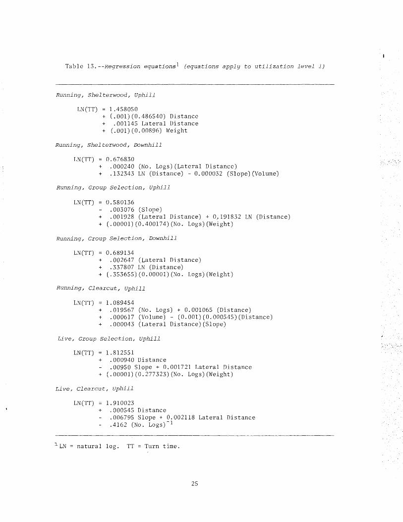
Table 13.--Regression equations 1 (equations apply to utilization level 1)
Running, Shelterwood, Uphill
LN(TT) 1.458050 + (.001)(0.486540) Distance + .001145 Lateral Distance + (.001)(0.00896) Weight
Running, Shelterwood, Downhill
LN(TT) 0.676830 + .000240 (No. Logs) (Lateral Distance) + .132343 LN (Distance) - 0.000032 (Slope)(Volume)
Running, Group Selection, Uphill
LN(TT) 0.580136 .003076 (Slope)
+ .001928 (Lateral Distance) + 0~191832 LN (Distance) + (.00001) (0.400174) (No. Logs) (Weight)
Running, Group Selection, Downhill
LN(TT) 0.689134 + .002647 (Lateral Distance) + .337807 LN (Distance) + (.353655)(0.0000l)(No. Logs)(Weight)
Running, Clearcut, Uphill
LN(TT) 1.089454 + .019567 (No. Logs) + 0.001065 (Distance) + .000617 (Volume) - (0.001)(0.000545)(Distance) + .000043 (Lateral Distance) (Slope)
Live, Group Selection, Uphill
LN(TT) 1.812551 + .000940 Distance
.00950 Slope + 0.001721 Lateral Distance + (.00001)(0.277323) (No. Logs)(Weight)
Live, Clearcut, Uphill
LN(TT) 1.910023 + .000545 Distance
.006795 Slope + 0.002118 Lateral Distance
.4162 (No. Logs)-1
1 LN natural log. TT Turn time.
25

Table 14.--Independent variables and their contributions to R2 for each regression equation (equations apply to utilization level 1)
Harvesting situation, regression equation
Dependent variable
Running Skyline, Shelterwood,
Uphill _!_/ LN (TT)
Running Skyline, Shelterwood,
Downhill
Running Skyline, Group Selection,
Uphill
Running Skyline, Group Selection,
Downhill
Running Skyline, Clearcut, Uphill
Live Skyline, Group Selection,
Uphill
l/ LN natural log. TT
LN(TT)
LN(TT)
LN(TT)
LN(TT)
LN(TT)
LN(TT)
turn time.
Independent variable and contribution to R2
Variable
Distance Lateral Distance
Weight
LN (Distance) (Slope) (Volume) (-)
(No. Logs) (Lateral Distance)
LN (Distance) Lateral Distance
(No. Logs) (Weight) Slope
LN (Distance) Lateral Distance
(No. Logs) (Weight)
Distance (Lateral Distance)
(Slope) Volume
(Distance) 2 (-) No. Logs
Distance Lateral Distance
Slope (-) (No. Logs) (Weight)
Distance (No. Logs)- 1 (-)
Lateral Distance Slope (-)
26
Contribution to R2
0.2957 . 0135 .0047
.2134
. 0353
.0257
.3787
.0375
.0348
. 0121
.1039
.0715
.0261
.2176
.0478
.0252
.0222
.0160
.2578
.0276
.0270
. Oll2
.2660
.0476
.0294
.0208
R2 for equation
0.34
.44
.68
. 32
.48
.42
.41

Table 15.--Turn time prediction factors, running, shelterwood, uphill
Matrix A
Lateral distance ft (m)
0 10 20 30 40 50 60 70 80 90 100 (3. 0) (6. 1) (9. 1) (12.2) (15. 2) (18. 3) (21.3) (24.4) (27.4) (30.5)
25 4.350 4.400 4.451 4.502 4.554 4.606 4.660 4.713 4.767 4.822 4.878 (7.6)
125 4.567 4.620 4.673 4. 727 4.781 4.836 4.892 4.948 5.005 5.063 5.121 (38.1)
225 4.795 4.850 4.906 4.962 5.019 5. 077 5.136 5.195 5.255 5.315 5.376 (68.6)
325 5.034 5.092 5.150 5. 210 5.270 5.330 5.392 5.454 5.517 5.580 5.644 (99. 1)
Skyline 425 5.285 5.346 5.407 5.469 5.532 5.596 5.661 5. 726 5. 792 5.858 5.926 distance (130.0) ft
(m) 525 5.548 5.612 5. 677 5.742 5.808 5.875 5. 943 6. 011 6.080 6. 150 6.221 (160. 0)
625 5.825 5.892 5.960 6.028 6.098 6.168 6.239 6. 311 6.384 6.457 6.531 (190. 0)
725 6.115 6.186 6.257 6.329 6.402 6.476 6.550 6.626 6. 702 6. 779 6.857 (221. 0)
825 6.420 6.494 6.569 6.645 6. 721 6. 798 6. 877 6.956 7.036 7. 117 7. 199 (252. 0)
925 6.740 6.818 6.896 6.976 7.056 7.137 7.220 7.303 7.387 7.472 7.558 (282. 0)
1025 7.076 7.158 7.240 7.324 7.408 7.493 7.580 7.667 7. 755 7.844 7.935 (312. 0)
1125 7.429 7.515 7.601 7.689 7. 777 7.867 7.957 8.049 8.142 8.236 8.330 (343.0)
Matrix B
Weight lb (kg)
30 1510 2990 4470 5950 7430 8910 10390 11870 13350 14830 (13.6) (685) (1356) (2028) (2699) (3370) ( 4042) (4713) (5384) (oOS6) (6729)
1.000 1. 014 1. 027 1. 041 1. 055 1.069 1. 083 1. 098 1. 112 1. 127 1.142
27

Table 16.--Turn time prediction factors, running, shelterwood, downhill
~latrix A
Lateral distance ft (m)
0 10 20 30 40 50 60 70 80 90 100 (3. 0) (6.1) (9. 1) (12.2) (15. 2) (18. 3) (21. 3) (24.4) (27.4) (30.5)
1 1.968 1. 972 1.977 1. 982 1. 987 1. 991 1.996 2.001 2.006 2.011 2.015 2 1.968 1. 977 1. 987 1.996 2.006 2.015 2.025 2.035 2.045 2.054 2.064 3 1.968 1.982 1.996 2.011 2.025 2.040 2.054 2.069 2.084 2.099 2.115
Number 4 1.968 1. 987 2.006 2.025 2.045 2.064 2.084 2.104 2.125 2.145 2.166 of 5 1.968 1.991 2.015 2.040 2.064 2.089 2.115 2.140 2.166 2.192 2.218
logs 6 1.968 1.996 2.025 2.054 2.084 2.115 2.145 2.176 2.208 2.240 2. 272 7 1.968 2.001 2.035 2.069 2.104 2.140 2.176 2.213 2.251 2.289 2.328 8 1.968 2.006 2.045 2.084 2.125 2.166 2.208 2.251 2.294 2.339 2.384 9 1.968 2. 011 2.054 2.099 2.145 2.192 2.240 2.289 2.339 2.390 2.442
10 1.968 2.015 2.064 2.115 2.166 2.218 2.272 2.328 2.384 2.442 2.501
Matrix B
Volume bd.ft. (m3)
5 30 55 80 105 130 155 180 205 230 255 (0.02) (0.14) (0.25) (0. 36) (0.48) (0.59) (0. 70) (0.82) (0.93) (1. 04) (1.16)
-30 1.005 1.029 1.054 1.080 1.106 1.133 1.160 1. 189 1. 218 1.247 1.277 -25 1.004 1.024 1.045 1.066 1.088 1.110 1.132 1.155 1.178 1. 202 1.226 -20 1.003 1. 019 1. 036 1. 053 1. 070 1. 087 1.104 1.122 1.140 1.159 1.177
Slope -15 1.002 1.015 1.027 1.039 1.052 1.064 1.077 1.090 1.103 1.117 1.130 (per- -10 1.002 1.010 1. 018 1.026 1.034 1. 042 1. 051 1.059 1.068 1. 076 1.085 cent) - 5 1. 001 1.005 1.009 1.013 1. 017 1.021 1.025 1.029 1.033 1. 037 1.042
0 1.000 1.000 1.000 1.000 1.000 1.000 1.000 1.000 1.000 1.000 1.000 5 .999 .995 .991 .987 .983 .979 .976 . 972 .968 .964 .960
10 .998 .990 .983 .975 .967 .959 .952 .944 .937 .929 .922 15 .998 .986 .974 .962 .951 .940 .928 .917 .906 .895 .885 20 .997 .981 .965 .950 .935 .920 .906 .891 .877 .863 .849
Matrix c
Distance ft (m)
25 105 185 265 345 425 505 585 665 745 825 (7.6) (32.0) (56.4) (80.8) (lOS) (130) (154) (178) (204) (227) (251)
1. 531 1.851 1.995 2.093 2.167 2.228 2.279 2.324 2.364 2.399 2. 432
28

Table 17.--Turn time prediction factors, running, group selection, uphill
Matrix A
Weight lb (kg)
200 1200 2200 3200 4200 5200 6200 7200 8200 9200 10200 (90. 7) (544) (998) (1452) (1905) (2359) (2823) (3266) (3720) (4173) ( 4627)
1 1.788 1.795 1.802 1.809 1. 817 1.824 1. 831 1. 838 1.846 1. 853 1. 861 2 1.789 1.804 1.818 1.833 1.847 1.862 1. 877 1.892 1.907 1.923 1. 938 3 1.791 1. 812 1.834 1.856 1. 879 1. 901 1. 924 1.948 1.971 1.995 2.019
Number 4 1. 792 1.821 1.850 1.880 1. 910 1. 941 1. 973 2.004 2.037 2. 070 2. 103 of 5 1.793 1.830 1.867 1.904 1. 943 1. 982 2.022 2.063 2.105 2.147 2.191
logs 6 1.795 1. 838 1. 883 1. 928 1. 976 2.024 2.073 2.123 2.175 2.228 2.282 7 1.796 1.847 1.900 1.954 2.009 2.066 2.125 2.185 2.248 2. 311 2. 377 8 1. 798 1.856 1. 917 1.979 2.043 2.110 2.178 2.249 2.323 2.398 2.476 9 1.799 1.865 1. 934 2.004 2.078 2.154 2.233 2.315 2.400 2.488 2.579
10 1. 801 1. 874 1. 951 2.030 2.113 2.199 2.289 2.383 2.480 2.581 2.687
Matrix B
Lateral Distance ft (m)
0 10 20 30 40 so 60 70 80 90 100 (3.0) (6 .1) (9. 1) (12.2) (15. 2) (18.3) (21.3) (24.4) (27.4) (30.5)
22 .935 .953 .971 .990 1.009 1.029 1.049 1. 070 1.090 1.112 1. 133 27 .920 .938 .956 .975 .994 1. 013 1. 033 1. 053 1. 074 1.095 1. 116 32 .906 .924 .942 .960 .979 .998 1. 017 1. 037 1. 057 1. 078 1.099 37 .892 .910 .928 .946 .964 .983 1.002 1.021 1. 041 1.062 1. 082
Slope 42 .879 .896 .913 .931 .949 .968 .987 1.006 1.025 1.045 1.066 (per- 47 .865 .882 .899 .917 .935 .953 . 972 .990 1. 010 1. 029 1.049 cent) 52 .852 .869 .886 .903 .921 .938 .957 .975 .994 1. 014 1. 033
57 .839 .856 .872 .889 .906 .924 .942 .960 .979 .998 1. 018 62 .826 .842 .859 .876 .893 .910 .928 .946 .964 .983 1.002 67 .814 .830 .846 .862 .879 .896 .914 .931 .949 .968 .987 72 .801 .817 .833 .849 .866 . 882 .900 .917 . 935 .953 . 972
Matrix c
Distance ft (m)
so 170 290 410 530 650 770 890 1010 1130 1250 (15.2) (51.8) (88.4) (125) (162) (198) (235) (271) (308) (344) (381)
2.118 2.678 2.967 3.171 3.331 3.464 3.579 3.679 3. 770 3.852 3. 927
29

Table 18.--Turn time prediction factors, running, group selection, downhill
Matrix A
Weight lb (kg)
250 1150 2050 2950 3850 4 750 5650 6550 7450 8350 9250 (113) (526) (930) (1338) (17 46) (2155) (2563) (2971) (3379) (3788) (4196)
2 0.503 0.506 0.509 0.513 0.516 0.519 0.522 0.526 0.529 0.533 0.536 3 .503 .508 .513 .518 .523 .528 .533 .538 .543 .549 .554 4 .504 .510 .517 .523 .530 .537 .544 .551 .558 .565 .572
Number 5 .504 .512 .521 .529 .537 .546 .555 .564 .573 .582 .591 of 6 .505 .514 .524 .534 .545 .555 .566 .577 .588 .599 . 611
logs 7 .505 .517 .528 .540 .552 .565 .577 .590 .604 .617 .631 8 .506 .519 .532 .546 .560 .574 .589 .604 .620 .636 . 652 9 .506 .521 .536 .551 .567 .584 .601 .618 .636 .655 .674
10 .506 .523 .540 .557 .575 .594 .613 .633 .653 .674 .696 11 .507 .525 .544 .563 .583 .604 .625 .648 .671 .695 . 719
Matrix B
Distance ft (m)
180 240 300 360 420 480 540 600 660 720 780 (54. 9) (73.2) (91.4) (llO) (128) (146) (165) (183) (201) (219) (238)
10 5.934 6.540 7.052 7.499 7.900 8.265 8.600 8.912 9.204 9.478 9. 738 (3.0)
20 6.093 6.715 7.241 7. 701 8.ll2 8.487 8.831 9.151 9.450 9. 732 9.999 (6. 1)
30 6.257 6.895 7.435 7.907 8.330 8. 714 9.068 9.396 9. 704 9.993 10.267 (9 .1)
Lateral 40 6.424 7.080 7.634 8.ll9 8.553 8.948 9. 3ll 9.649 9.964 10.261 10.543 distance
ft (12.2)
(m) so 6.597 7. 270 7.839 8.337 8. 783 9.188 9.561 9.907 10.232 10.537 10.826 (15.2)
60 6. 774 7.465 8.049 8.561 9.018 9.434 9.817 10.173 10.506 10.819 ll.ll6 (18.3)
70 6.955 7.665 8.265 8.790 9.260 9.688 10.081 10.446 10.788 ll.llO 11.414 (21. 3)
80 7.142 7.871 8.487 9.026 9.509 9.947 10.351 10.726 11. 077 11.408 11. 720 (24. 4)
90 7.333 8.082 8.715 9.268 9. 764 10.214 10.629 11. 014 11. 374 11. 714 12.035 (27. 4)
100 7.530 8.299 8.948 9.517 10.026 10.488 10.914 11. 309 11.679 12.028 12.357 (30.5)
30

Table 19.--Turn time prediction factors, running, clearcut, uphill
Matrix A
Volume bd.ft. (m3)
5 25 45 65 85 105 125 145 165 185 205 (0. 02) (0.11) (0.20) (0.29) (0.38) (0.48) (0.57) (0.66) (0.75) (0.84) (0.93)
60 3.172 3.212 3.252 3.293 3.334 3.375 3.417 3.460 3.503 3.579 3.591 (18.3)
145 3.440 3.483 3.527 3. 571 3.615 3.660 3.706 3.752 3.799 3.846 3.894 (44.2)
230 3.701 3. 74 7 3.794 3.842 3.889 3.938 3.987 4.037 4.087 4.138 4.190 (70.1)
315 3.951 4.000 4.050 4.101 4.152 4.204 4.256 4.309 4.363 4.417 4.473 (96.0)
Distance 400 4.184 4.237 4.289 4.343 4.397 4.452 4.508 4.564 4.621 4.678 4.737 ft (122)
(m) 485 4.397 4.452 4.507 4.563 4.620 4.678 4.736 4.796 4.855 4.916 4. 977
(148)
570 4.584 4.641 4.699 4. 758 4.817 4. 877 4.938 4.999 5.062 5.125 5. 189 (174)
655 4.741 4.800 4.860 4.921 4.982 5.045 5.108 5.171 5.236 5.301 5.367 (200)
740 4.866 4.926 4.988 5.050 5.113 5.177 5.242 5.307 5.373 5.440 5.508 (226)
825 4.954 5.016 5.079 5.142 5.206 5. 271 5.337 5.403 5.471 5.539 5.608 (251)
910 5.005 5.067 5.130 5.194 5.259 5.325 5.391 5.459 5.527 5.596 5.665 (277)
Matrix B
Lateral distance ft (m)
0 10 20 30 40 50 60 70 80 90 100 (3.0) c 6. 1) (9. 1) (12.2) (15.2) (18. 3) (21. 3) (24.4) (27.4) (30.5)
20 1.000 1.009 1.017 1.026 1.035 1.044 1. 053 1.062 1. 071 1.080 1. 090 25 1. 000 1. 011 1. 022 1. 033 1. 044 1. 055 1. 067 1.078 1.090 1. 102 1.113 30 1.000 1.013 1.026 1.039 1. 053 1. 067 1. 080 1.095 1.109 1.123 1.138
Slope 35 1.000 1. 015 1. 031 1.046 1. 062 1.078 1.095 1.111 1.128 1.145 1. 162 (per- 40 1.000 1. 017 1.035 1. 053 1. 071 1.090 1.109 1.128 1.148 1.167 1. 188 cent) 45 1.000 1. 020 1. 039 1.060 1.080 1.102 1.123 1. 145 1.167 1.190 1.213
50 1.000 1. 022 1.044 1.067 1. 090 1.113 1.138 1.162 1. 188 1. 213 1. 240 55 1.000 1. 024 1. 048 1. 074 1.099 1.126 1.152 1.180 1. 208 1. 237 1. 267 60 1.000 1. 026 1. 053 1.080 1.109 1.138 1.167 1.198 1. 229 1. 261 1.294
Matrix c
Number of logs
2 3 4 5 6 7 8 9 10
1.020 1.040 1. 060 1. 081 1.103 1.125 1. 14 7 1.169 1.193 1. 261
31

Table 20.--Turn time prediction factors, live, group selection, uphill
~-latrix A
Lateral distance ft (m)
0 10 20 30 40 50 60 70 80 90 100 (3.0) (6.1) (9 .1) (12.2) (15. 2) (18. 3) (21.3) (24.4) (27.4) (30.5)
40 4.189 4.262 4.336 4. 411 4.488 4.566 4.645 4. 726 4.808 4.891 4.976 45 3.995 4.064 4.135 4.207 4.280 4.354 4.430 4.506 4.585 4.664 4.745
Slope 50 3.810 3.876 3.943 4.012 4.081 4.152 4.224 4.297 4. 372 4.448 4.525 (per- 55 3.633 3.696 3.760 3.825 3.892 3.959 4.028 4.098 4.169 4.242 4.315 cent) 60 3.464 3.525 3.586 3.648 3. 711 3. 776 3.841 3.908 3.976 4.045 4.115
65 3.304 3.361 3.419 3.479 3.539 3.601 3.663 3.727 3.791 3.857 3.924 70 3.150 3.205 3.261 3.317 3.375 3.434 3.493 3.554 3.615 3. 678 3.742
~1atrix B
Weight lb (kg)
75 875 1675 2475 3275 4075 4875 5675 6475 7275 8075 (34. 0) (397) (760) (1123) (1486) (1848) (2211) (2574) (2937) (3300) (3663)
1 1. 000 1.002 1.005 1.007 1.009 1.011 1. 014 1. 016 1. 018 1. 020 1. 023 2 1.000 1.005 1.009 1.014 1. 018 1. 023 1. 027 1.032 1. 037 1. 041 1.046 3 1.001 1.007 1. 014 1. 021 1. 028 1.034 1. 041 1.048 1.055 1.062 1.069 4 1.001 1. 010 1. 019 1. 028 1. 037 1.046 1.056 1.065 1. 074 1.084 1.094
Number 5 1.001 1. 012 1. 023 1.035 1.046 1. 058 1. 070 1.082 1.094 1. 106 1.118 of 6 1. 001 1.015 1.028 1.042 1.056 1.070 1.084 1.099 1.114 1.129 1. 144
logs 7 1.001 1. 017 1.033 1.049 1.066 1. 082 1.099 1.116 1. 134 1. 152 1. 170 8 1.002 1.020 1. 038 1.056 1. 075 1. 095 1.114 1.134 1.154 1.175 1.196 9 1.002 1. 022 1. 043 1.064 1.085 1.107 1. 129 1. 152 1. 175 1.199 1. 223
10 1. 002 1. 025 1. 048 1. 071 1. 095 1.120 1.145 1.170 1. 197 1. 224 1. 251 11 1.002 1. 027 1. 052 1. 078 1.105 1.132 1.160 1.189 1. 218 1. 248 1.279 12 1.002 1.030 1.057 1.086 1.115 1.145 1.176 1. 208 1.240 1. 274 1. 308
Matrix c ..
Distance ft (m)
50 125 200 275 350 425 500 575 650 725 800 (15.2) (38.1) (61. 0) (83.8) (107) (130) (152) (175) (198) (2 21) (244)
1.048 1.125 1. 207 1.295 1.390 1. 491 1.600 1. 717 l. 842 1. 977 2.121
32

Table 21.--Turn time prediction factors, live, clearcut, uphill
fvlatrix A
Lateral distance ft (rn)
0 10 20 30 40 50 60 70 80 90 100 (3. 0) (6 .1) (9. l) (12.2) (15.2) (18.3) (21. 3) (24. 4) (27.4) (30.5)
10 6.790 6.935 7.084 7.236 7.390 7.549 7. 710 7.875 8.044 8.216 8.392 (3. 0)
90 7.093 7.245 7.400 7.558 7. 720 7.885 8.054 8.226 8.402 8.582 8. 766 (27.4)
170 7.409 7.567 7. 729 7.895 8.064 8.236 8.413 8.593 8. 777 8.965 9.157 (51.8)
250 7.739 7.905 8.074 8.247 8.423 8.604 8. 788 8.976 9.168 9.364 9.565 (76. 2)
330 8.084 8.257 8.434 8.614 8. 799 8.987 9.179 9.376 9. 577 9. 781 9.991 (101)
410 8.444 8.625 8.810 8.998 9.191 9.387 9.588 9.794 10.003 10.217 10.436 (125)
Distance 490 8.820 9.009 9.202 9.399 9.600 9.806 10.016 10.230 10.449 10.637 10.901
ft (rn) (149)
570 9.214 9.411 9.612 9.818 10.028 10.243 10.462 10.686 10.915 11. 148 11.387 (174)
650 9.624 9.830 10.041 10.255 10.475 10.699 10.928 11.162 11.401 11. 645 11.894 (198)
730 10.053 10.268 10.488 10.713 10.942 11. 176 11.415 11.660 11.908 12.164 12.425 (223)
810 10.501 10.726 10.955 11.190 11.429 11.674 11. 924 12.179 12.440 12.706 12.978 (24 7)
890 10.969 11.204 11.444 11.689 11.939 12.194 12.455 12.722 12.994 13.272 13.557 (271)
970 11.458 11. 703 11.954 12.209 12.471 12.738 13.010 13.289 13.573 13.864 14.161 (296)
Matrix B
Number of logs
2 3 4 5 6 7 8 9 10
45 0.486 0.598 0.641 0.664 0.678 0.687 0.694 0.699 0. 703 0. 707 Slope so .470 .578 .620 .642 .655 .664 .671 .676 .680 .683 (per- 55 .454 .559 .599 .620 .633 . 642 .648 .653 .657 . 660 cent) 60 .439 .540 .579 .599 .612 .621 .627 .631 .635 .638
65 .424 .522 .560 .579 .592 .600 .606 .610 .614 .617 70 .410 .505 .541 .560 .572 .580 .586 .590 .593 .596
33

Table 22.--Total foreign element statistics. (Foreign elements are delays attributed to machines, manpower, material, and environmental factors)
System
Running Skyline Shelterwood Uphill
Running Skyline Shelterwood Downhill
Running Skyline Group Selection Uphill
Running Skyline Group Selection Downhill
Running Skyline Clearcut Uphill
Live Skyline Group Selection Uphill
Live Skyline Clearcut Uphill
Turns with foreign elements
Percent
30.6
27.7
40.7
14.7
15.7
20.0
19.6
34
Av. total foreign element time in
turns with foreign elements
Minutes
28.0
3.8
2.5
2.2
3.0
11.0
3.2
Av. foreign element time for all turns
Percent
14.4
23.7
26.3
6.4
8.2
27.8
10.8

Turn time (min)
3.0
.2
. 4
.6
.8
4.0
.2
.4
.6
. 8
5.0
. 2
.4
.6
. 8
6.0
.2
. 4
.6
.8
7.0
.2
.4
.6
. 8
8.0
Table 23.--Cubic foot (m 3 ) volume per hour for turn times given piece size and number of logs
4.0 Log/Load
10 12 14 16 18 20 (0.24) (0.29) (0.33) (0.38) (0.43) (0.48)
800 960 1120 1280 1440 1600 (22.6) (27.2) (31.7) (36.2) (40.8) (45.3)
750 900 1050 1200 1350 1500 (21.2) (25.5) (29.7) (34.0) (38.2) (42.5)
706 847 988 1129 1271 1412 (20.0) (24.0) (27.9) (32.0) (36.0) (40.0)
667 800 933 1067 1200 1333 (18.9) (22.6) (26.4) (30.2) (34.0) (37.8)
637 756 884 1010 1137 1263 (18.0) (21.4) (25.0) (28.6) (.)2.2) (35.8)
600 720 840 960 1080 1200 (17.0) (20.4) (23.8) (27.2) (30.6) (34.0)
571 686 800 914 1029 1143 (16.2) (19.4) (22.6) (25.9) (29.1) (32.4)
546 655 764 873 982 1091 (15.5) (18.5) (21.6) (24.7) (27.8) (30.9)
522 626 730 835 939 1043 (14.8) (17.7) (20.7) (23.6) (26.6) (29.5)
500 600 700 800 900 1000 (14.2) (17.0) (19.8) (22.6) (25.5) (28.3)
480 576 672 768 864 960 (13.6) (16.3) (19.0) (21.7) (24.5) (27.2)
462 554 646 738 831 923 (13.1) (15.7) (18.3) (20.9) (23.5) (26.1)
444 533 622 711 800 889 (12.6) (15.1) (17.6) (20.1) (22.6) (25.2)
429 514 600 686 771 857 (12.1) (14.6) (17.0) (19.4) (21.8) (24.3)
414 497 579 662 745 828 (11.7) (14.1) (16.4) (18.7) (21.1) (23.4)
400 480 560 640 720 800 (11.3) (13.6) (15.9) (18.1) (20.4) (22.6)
387 464 542 619 697 774 (ll.O) (13.1) (15.3) (17.5) (19.7) (21.9)
375 450 525 600 675 750 (10.6) (12.7) (14.9) (17.0) (19.1) (21.2)
364 436 509 582 655 727 (10.3) (12.3) (14.4) (16.5) (18.5) (20.6)
353 423 494 565 635 706 (10.0) (12.0) (14.0) (16.0) (18.0) (20.0)
343 411 480 549 617 686 (9.7) (11.6) (13.6) (15.5) (17.5) (19.4)
333 400 467 533 600 667 (9.4) (11.3) (13.2) (15.1) (17.0) (18.9)
324 389 454 519 584 649 (9.2) (11.0) (12.9) (14.7) (16.5) (18.4)
316 379 442 505 568 632 (8.9) (10.7) (12.5) (14.3) (16.1) (17.9)
308 369 431 492 554 615 (8.7) (10.5) (12.2) (13.9) (15.7) (17.4)
300 360 420 480 540 600 (8.5) (10.2) (11.9) (13.6) (15.3) (17.0)
35
5.0 Log/Load
10 12 14 16 18 20 (0.24) (0.29) (0.33) (0.38) (0.43) (0.48)
1000 1200 1400 1600 1800 2000 (28.3) (34.0) (39.7) (45.3) (51.0) (56.6)
938 1125 1312 1500 1688 1875 (26.6) (31.9) (37.2) (42.5) (47.8) (53.1)
882 1059 1235 1412 1588 1765 (25.0) (30.0) (35.0) (40.0) (45.0) (50.0)
833 1000 1167 1333 1500 1667 (23.6) (28.3) (33.1) (27.8) (42.5) (47.2)
789 947 1105 1263 1421 1579 (22.3) (26.8) (31.3) (35.8) (40.2) (44.7)
750 900 1050 1200 1350 1500 (21.2) (25.5) (29.7) (34.0) (38.2) (42.5)
714 857 1000 1143 1286 1429 (20.2) (24.3) (28.3) (32.4) (36.4) (40.5)
682 818 955 1091 1228 1364 (19.3) (23.2) (27.0) (30.9) (34.9) (38.6)
652 782 913 1043 1174 1304 (18.5) (22.1) (25.9) (29.5) (33.2) (36.9)
625 750 875 1000 1125 1250 (17.7) (21.2) (24.9) (28.3) (31.9) (35.4)
600 720 840 960 1080 1200 (17.0) (20.4) (23.8) (27.2) (30.6) (34.0)
577 692 808 923 1038 1154 (16.3) (19.6) (22.9) (26.1) (29.4) (32.7)
556 667 778 889 1000 1111 (15.7) (18.8) (22.0) (25.2) (28.3) (31.5)
536 643 750 857 964 1071 (15.2) (18.2) (21.2) (24.3) (27.3) (30.3)
517 621 724 828 931 1034 (14.6) (17.6) (20.5) (23.4) (26.4) (29.3)
500 600 700 800 900 1000 (14.2) (17.0) (19.8) (22.6) (25.5) (28.3)
484 (13. 7)
581 677 774 871 968 (16.5) (19.2) (21.9) (24.7) (27.4)
469 562 656 750 844 938 (13.3) (15.9) (18.6) (21.2) (23.9) (26.6)
455 545 636 728 819 909 (12.9) (15.4) (18.0) (20.6) (23.2) (25.7)
441 529 618 706 794 882 (12.5) (15.0) (17.5) (20.0) (22.5) (25.0)
429 514 600 686 771 857 (12.1) (14.6) (17.0) (19.4) (21.8) (25.3)
417 500 583 667 750 833 (11.8) (14.2) (16.5) (18.9) (22.1) (23.6)
405 486 568 649 730 811 (11.5) (13.8) (16.1) (18.4) (20. 7) (23.0)
395 474 553 632 711 790 (11.2) (13.4) (15.7) (17.9) (20.1) (22.4)
385 461 538 616 692 769 (10.9) (13.1) (15.2) (17.4) (19.6) (21.8)
375 450 525 600 675 750 (10.6) (12.7) (14.9) (17.0) (19.1) (21.2)

Gardner, Rulon B. 1980. Skyline logging productivity under alternative
harvesting prescriptions and levels of utilization in larch-fir stands. USDA For. Serv. Res. Pap. INT-247, 35 p. Intermt. For. and Range Exp. Stn., Ogden, Utah 84401.
Larch-fir stands in northwest Montana were experimentally logged to determine the influence of increasingly intensive levels of utilization upon rates of yarding production, under three different silvicultural prescriptions. Variables influencing rate of production were also identified.
KEYWORDS: Skyline yarding, productivity, utilization.
Gardner, Rulon B. 1980. Skyline logging productivity under alternative
harvesting prescriptions and levels of utilization in larch-fir stands. USDA For. Serv. Res. Pap. INT- 247, 35 p. Intermt. For. and Range Exp. Stn., Ogden, Utah 84401.
Larch-fir stands in northwest Montana were experimentally logged to determine the influence of increasingly intensive levels of utilization upon rates of yarding production, under three different silvicultural prescriptions. Variables influencing rate of production were also identified.
KEYWORDS: Skyline yarding, productivity, utilization.


The Intermountain Station, headquartered in Ogden, Utah, is one of eight regional experiment stations charged with providing scientific knowledge to help resource managers meet human needs and protect forest and range ecosystems.
The Intermountain Station includes the States of Montana, Idaho, Utah, Nevada, and western Wyoming. About 231 million acres, or 85 percent, of the land area in the Station territory are classified as forest and rangeland. These lands include grasslands, deserts, shrublands, alpine areas, and well-stocked forest~. They supply fiber for forest industries; minerals for energy and industrial development; and water for domestic and industrial consumption. They also provide recreation opportunities for millions of visitors each year.
Field programs and research work units of th~ Station are maintained in:
Boise, Idaho
Bozeman, Montana (in cooperation with Montana State University)
Logan, Utah (in cooperation with Utah State University)
Missoula, Montana (in cooperation with the University of Montana)
Moscow, Idaho (in cooperation with the University of Idaho)
Provo, Utah (in cooperation with Brigham Young University)
Reno, Nevada (in cooperation with the University of Nevada)
FOREST RESIDUES UTILIZATION RESEARCH AND DEVELOPMENT PROGRAM