SKF Freight Transports and CO2 emissions a Study in Environmental Management Accounting Master of Science Thesis Helen Lindblom & Christian Stenqvist Department of Energy and Environment Division of Environmental Systems Analysis CHALMERS UNIVERSITY OF TECHNOLOGY Göteborg, Sweden 2007 ESA Report 2007: 18 ISSN 1404-8167

ESA Report 2007: 18

SKF Freight Transports and CO2 emissions a Study in Environmental Management Accounting

Helen Lindblom and Christian Stenqvist

Department of Energy and Environment CHALMERS UNIVERSITY OF TECHNOLOGY

Göteborg Sweden 2007

SKF Freight Transports and CO2 emissions a Study in Environmental Management Accounting HELEN LINDBLOM & CHRISTIAN STENQVIST © Helen Lindblom and Christian Stenqvist, 2007 ESA Report 2007: 18 ISSN 1404-8167 Department of Energy and Environment Division of Environmental Systems Analysis Chalmers University of Technology SE- 412 96 Göteborg Sweden Telephone: +46 (0)31 7721000 Chalmers Reproservice Göteborg, Sweden 2007

Executive Summary Emissions of greenhouse gases, foremost carbon dioxide, causing human induced climate change have become a global and fateful issue. All parties ought to be engaged in the mission of mitigating the anticipated impacts. For any organization determined to deal with the issue, measuring its carbon footprint is an essential step to take. Since 2001 SKF has monitored the level of CO2 emissions associated with its manufacturing processes. Included in this scope are the CO2 emissions originating from electricity, heat and fuel consumption at the production sites and other facilities. During these years the emissions figures have been published in the annual sustainability report, from which it is evident that SKF has managed to reduce the group’s total CO2 emissions. This is in line with the annual CO2 reduction targets, and in a carbon constrained future it should be seen as a competitive advantage to continue on this route. CO2 emissions from transportation of SKF goods and staff have so far been kept outside the monitoring scope. These sources are expected to contribute significantly to the total carbon impact of a multinational manufacturing company like SKF, and hence they should also be monitored and managed. In this study of CO2 emissions accounting, SKF freight transports are examined. The identification of emission sources, the handling of transport activity data, the application of proper calculation methodologies, organizational aspects and questions of liability are all integrated parts of the study. Emission calculations are carried out for two specific logistics systems managed by SKF Logistics Services; the Daily Transport System (DTS) and the Global Air Freight Program. The DTS, which is based on road freight transports, operates the European distribution of finished products. It is estimated to contribute with 9 700 tonnes CO2 during 2007. Since the system is optimized to a reasonable degree, the CO2 impact per tonne-km is relatively low. Over the same period the air freight’s estimated emissions are 40 000 tonnes. Together these transport activities contributes to about ten percent of the SKF total CO2 equivalents based on the reporting of 2006. Adding the emissions from the remaining transport activities that SKF utilizes will make this share increase considerably, particularly if also inbound transports are accounted for. The potential for CO2 reductions is covered by two change-oriented case studies. It can be concluded that short-sea transportation seldom is an alternative to road transports. Intermodal transports combining road and rail can, depending on the circumstances, reduce the CO2 impact considerably compared to only using road transports. Reducing transportation work by optimizing a transport activity is seen as the best option for CO2 reductions. Efforts should be put into reducing the need for air freight transports, considering the high emission levels per tonne-km. Monitoring emissions for all transport activities that falls under SKF responsibility will reduce the risk of sub optimization. Introducing system changes in order to decrease CO2 emissions will have a range of implications for all actors involved. Effects on lead-time, cost and warehousing capability are some of the factors that will have to be further analyzed. Other barriers to introducing system changes can be lack of knowledge, resources and available transport options.

Acknowledgements This study is the final part of our engineering studies. The thesis has been carried out at the department of Environmental Systems Analysis at Chalmers University of Technology and at SKF. First of all, we would like to thank our academic supervisors; Karl Hillman, Örjan Lundberg and our examiner Bengt Steen, for valuable comments regarding our work. Birger Löfgren also contributed with many interesting thoughts. We are also grateful for all help given by Magnus Swahn and Magnus Blinge at NTM, the Network for Transport and Environment. At SKF, we would like to thank; Lennart Karlsson, Transport Coordination Manager East Europe and Middle East, SKF Logistics Services Ulf Andersson, Environmental Coordinator, SKF Sweden Rob Jenkinson, Project Manager Group Sustainability for their help with practical issues as well as with information needed for the study. Thanks also to; Yngve Ohlsson, Vice President Transports, SKF Logistics Services Mattias Axelsson, Manager Quality, Packaging and Administration Services, SKF Logistics Services Gothenburg Martin Eliasson, Global Product Manager Airfreight, SKF Logistics Services Jonas Dahlqvist, CTT Manager, SKF Logistics Services Magnus Wellsted, Controller Business Area Transport, SKF Logistics Services Juergen Toepfer, Global Product Manager Road Freight, SKF Logistics Services and other persons at SKF Logistics Services for their support. Gothenburg, November 2007 Helen Lindblom Christian Stenqvist

Table of Contents 1. INTRODUCTION .................................................................................................................................... 1

1.1 BACKGROUND ...................................................................................................................................... 1

1.2 PURPOSE ............................................................................................................................................... 1

1.3 METHODOLOGY .................................................................................................................................... 2

1.4 DELIMITATIONS .................................................................................................................................... 3

1.5 PREVIOUS STUDIES ............................................................................................................................... 4 1.6 GUIDE FOR READERS ............................................................................................................................. 5

2 SETTING THE SCENE ............................................................................................................................ 6

2.1 SKF AND SKF LOGISTICS SERVICES..................................................................................................... 6

2.2 FREIGHT TRANSPORTS .......................................................................................................................... 6 2.2.1 Trends .......................................................................................................................................... 6

2.2.2 Challenges ................................................................................................................................... 8

2.3 TRANSPORT EMISSIONS ......................................................................................................................... 9 2.3.1 Greenhouse effect and global warming ....................................................................................... 9 2.3.2 Other transport emissions .......................................................................................................... 10

2.3.3 Carbon dioxide emissions from different transport modes ........................................................ 11 2.4 ENVIRONMENTAL MANAGEMENT ....................................................................................................... 12

2.4.1 Environmental Management in theory ....................................................................................... 12 2.4.2 Environmental Management in practice .................................................................................... 13

3 ACCOUNTING PROCEDURE ............................................................................................................. 16

3.1 AUDIT ................................................................................................................................................. 16

3.1.1 Environmental Management and transport ............................................................................... 16 3.1.2 Where are we? - Environmental Management at SKF ............................................................... 17 3.1.3 Where are the others? ................................................................................................................ 19

3.2 STRATEGY .......................................................................................................................................... 21

3.2.1 Where do we want to be? ........................................................................................................... 21

3.2.2 Who should we tell? ................................................................................................................... 23

3.3 ACTION PLAN ..................................................................................................................................... 24

3.3.1 Identify sources .......................................................................................................................... 25

3.3.2 Select Calculation Approach...................................................................................................... 27

3.3.3 Collect Data and Choose Emission Factors .............................................................................. 28 3.3.4 Apply Calculation Tools ............................................................................................................. 33

3.3.5 Roll-up Data to Corporate Level ............................................................................................... 34

4. MAPPING A LOGISTICS SYSTEM .................................................................................................. 35

4.1 SYSTEM DESCRIPTION ......................................................................................................................... 35 4.2 ASSUMPTIONS ..................................................................................................................................... 38

4.2.1 Method ....................................................................................................................................... 38

4.2.2 Transport activity data for road transports ............................................................................... 39 4.2.3 Transport activity data and calculation methods for other modes ............................................. 40

4.3 RESULTS ............................................................................................................................................. 41

4.3.1 Daily Transport System .............................................................................................................. 41

4.3.2 DTS compared to air freight ...................................................................................................... 42

4.4 ANALYSIS ........................................................................................................................................... 44

4.4.1 Sensitivity analysis ..................................................................................................................... 44

4.4.2 Analysis of method choices ........................................................................................................ 46

4.4.3 Uncertainty of SKF and supplier data ....................................................................................... 50

5 CASE STUDIES – IMPROVING A LOGISTICS SYSTEM .............................................................. 53

5.1 CASE GOTG – INTERMODAL TRANSPORT ........................................................................................... 53

5.2 CASE UK – DECREASING TRANSPORT WORK ....................................................................................... 55

6 DISCUSSION ........................................................................................................................................... 57

7 FINAL CONCLUSIONS ........................................................................................................................ 61

8 REFERENCES ........................................................................................................................................ 62

APPENDIX 1 ................................................................................................................................................. I

APPENDIX 2 ............................................................................................................................................... II

APPENDIX 3 .............................................................................................................................................. III

APPENDIX 4 .............................................................................................................................................. IV

APPENDIX 5 ................................................................................................................................................ V

APPENDIX 6 .............................................................................................................................................. VI

APPENDIX 7 .............................................................................................................................................VII

1

1. Introduction

1.1 Background “…for their effort to build up and disseminate greater knowledge about man-made climate change, and to lay the foundations for the measures that are needed to counteract such changes.”(The Nobel Foundation 2007) Not surprisingly the Nobel Peace Prize 2007 was awarded the Intergovernmental Panel on Climate Change (IPCC) and the former US vice president Al Gore. However, the scientific foundation has a long history; in 1896 Arrhenius published his findings on the relation between the atmospheric carbon dioxide (CO2) concentration and the global mean temperature (Arrhenius 1896). A century later IPCC, founded in 1988, has published a series of assessment reports that summarize the state of knowledge on the issue. Meanwhile, Gore and other advocates have been communicating their message to the broader public. Along with this intensified focus on climate change, the interest for corporate accounting of greenhouse gas (GHG) emissions has increased. For some years SKF has focused on monitoring and reducing CO2 emissions from stationary sources (SKF Annual report 2006). In addition, there is today a strong mandate in the organization to also include transports (of both goods and staff) in the accounting of GHG emissions (Jenkinson 2007). However, since this interest for transport emission accounting is rather new, the existing guidelines and methods are not giving full support to companies. The difficulty of measuring indirect environmental aspects, reflecting that SKF is a buyer and not the owner of its transport activities, further contributes to the complexity. This situation is shared by many other manufacturing companies with significant transport demands. Hence the issue raises several questions, e.g.: Which raw data should be used? How should the calculations be done? What should be reported? This study will examine these issues and thereby contribute with a guide to transport emissions accounting and the problems associated with it.

1.2 Purpose The purpose of this report is to explore the possibilities for monitoring CO2 emissions from freight transport, from a manufacturing company’s perspective. With a clear focus on SKF freight transport activities it covers the areas of; transport data handling, emission calculation methodology, and emission accounting principles. The study will provide answers to the following research questions: 1. What are the driving forces behind accounting for CO2 emissions from freight transport? 2. How can environmental impact from freight transport be handled by the environmental management system? 3. How should CO2 emissions from freight transports be calculated? 4. How can SKF’s transport systems be adjusted to decrease CO2 emissions?

2

1.3 Methodology A variety of methods have been addressed in order to answer the research questions and these are discussed in this section. Literature studies Companies’ interest for accounting CO2 emissions from their freight transports is a rather new and evolving field. To understand the driving forces behind this newborn interest a number of sources have been addressed. By publishing the scientific foundation on greenhouse gases and human induced climate change IPCC makes an important contribution. Apart from scientific proofs, the discussions on climate change cover aspects such as socioeconomic consequences and possible political measures. Related to freight transport, figures on state and trends within the sector are provided by official statistics. Prominent sources are provided from OECD and its energy organ the International Energy Agency (IEA), as well as the European Commission’s statistics from Eurostat. Literature studies also have importance for the discussion on environmental management systems (EMS), which is the tool used by the corporate world for working with environmental issues. EMS is also an academic field and by addressing relevant research the second question in the purpose can partly be answered. Personal communication A number of interviews have been conducted. They are all semi-structured, meaning some topics and questions have been prepared in beforehand, while others have been raised through the dialogues with the informants. Interviewing with the semi-structured approach has been judged appropriate since it encourages a two-way communication so that also the informants can bring up questions of interest. The informants are mainly SKF employees at different departments. Also academic experts in the field of logistics have been interviewed. When searching for specific transport data it has sometimes been found necessary to turn directly to transport suppliers, or other actors, for answers. Such occasional contact has been made by e-mail. Questionnaire SKF´s logistics unit has agreements with some 30 forwarding agents in Europe. On suspicion that these might provide transport data differing from that in the SKF data systems as well as in standardized emission calculation manuals, it was decided to do a questionnaire study. The questionnaire, presented in appendices 2 and 3, was e-mailed to the contact person at each forwarding agent. It was then passed on to an employee in position to answer the questions, who then replied with the filled-out form. For those agents not answering, a reminder was sent out. In the end, answers of varying quality were received from 55 percent of the forwarding agents.

3

Calculation methodology The area of emission calculation has been mapped to find examples on “best practice”. The Swedish association “the Network for Transport and Environment” (NTM) and the Greenhouse Gas Protocol, which is a partnership between the World Resources Institute and the World Business Council for Sustainable Development, are two frequently referenced sources providing the industry sector with CO2 emission calculation tools and manuals. Both have provided input to the discussions on calculation approaches as well as to the actual calculations.

Benchmarking CO2 emission management is an evolving field within the corporate world, and in recent years a number of business initiatives have been launched in the name of climate change. A few of these initiatives have been looked at since they are thought to give a picture of the business culture that surrounds global warming. They also say something about the position of the corporate collective in relation to the issue. Some companies are of course ahead of others in the ambitions on CO2

emission management. A few have been found to state examples on good practices. The participation at a full-day seminar about sustainable transports is also considered to be a valuable experience. The seminar, organized by IVL Swedish Environmental Research Institute in cooperation with NTM, gathered some essential actors from the industry and the transport sector, which gave their views on emission mitigation.

1.4 Delimitations This study will focus on freight transports of finished products, i.e. only the outbound flow of goods. Apart from a minor study on global air freight, the geographical boundary will be transports within Europe. However, transports outside Europe can be handled according to the same structure as presented in this study. All transport modes will be included in this study, although the focus will be on road and short sea transports. The accounting of air and rail transports will be covered in a general sense, but is not the primary focus. For a further discussion about air transportation at SKF, a previous study on SKF’s business travels is recommended (Johansson & Mellqvist 2007). Goods handling activities, e.g. by forklift trucks, conveyer belts etc, are kept outside the scope. These activities are often electric powered and the energy need is thereby covered by the total electricity demand of the factory or warehouse. The CO2 emissions from the production of electricity used at SKF’s units are already included in SKF’s CO2 accounting today. Since greenhouse gases are the main focus for SKF on a global corporate level (SKF intranet 2007) and CO2 by far is the most dominating greenhouse gas for the transport sector, only CO2 emissions will be considered in this study. In 2005, carbon dioxide accounted for more than 98 percent of the total greenhouse gas emissions from the transport sector (EEA 2007, Swedish EPA 2007).

4

Another reason for only including carbon dioxide is that this study focuses on the organizational and operational structure of the accounting process itself. The accounting procedure will be the same for any type of emission, and hence one type is enough to state an example. Other emissions, e.g. nitrogen oxides (NOx) and particles are of course important as well and it could be relevant for SKF to consider all transport emissions in their further work within this area. In SKF’s current CO2 reporting the lifecycle perspective is not considered. A lifecycle perspective means that the product is followed from the extraction all the way to the disposal (Baumann & Tillman 2004). A lifecycle perspective can be important for the result when accounting for transport emissions, especially if the purpose is to compare vehicles with different propulsion, e.g. a diesel fueled truck compared to a bio-fueled truck (Blinge 1998). In this study, the calculations will be done without a lifecycle perspective in order to be able to compare the results with SKF’s current emissions accounting. Hence the impact from other parts of the lifecycle will only be mentioned briefly. The discussions in the study are limited to a transport buyer perspective, in this case SKF and specifically SKF Logistics Services.

1.5 Previous studies Lifecycle assessments of specific products have been done at SKF for many years. One example is the study made by Ekdahl (2001) on spherical roller bearings. However, in these studies, transports have not been the main focus even though it is included in the assessments. At least one study at SKF, made by Carlsson et. al in 2003, has compared different transport modes for outbound transports, but it is not being done on a regular basis. Local initiatives exist, but there is no central monitoring of transport emissions or any standard on how comparative studies should be carried out. Connected to this study is the report made by Johansson and Mellqvist in 2007, which discusses sustainability issues connected to SKF’s business travels. Their report can serve as a complement when discussing the total impact of indirect emissions from the SKF group. In the scientific field, extensive research has been made where logistics and environmental implications have been connected. There are also standards and methods developed for companies, e.g. the Greenhouse Gas Protocol and the Global Reporting Initiative. Both are used by SKF today. Each field of study contributes to this specific report, but none of them have a practical method of how accounting of transport emissions should be carried out for a transport buying company. It is in this area this study hopefully will make a contribution.

5

1.6 Guide for readers The study consists of four quite detached parts (chapter two to five) which can be read consecutively or separately depending on the reader’s interest. In the second chapter; Setting the scene, a background to SKF, transportation dilemmas and environmental problems connected to transportation is presented, as well as an introduction to environmental management. In the third chapter; Accounting procedure, the study moves from the theoretical framework into a more practical method description of the accounting process. Benchmarking and strategy is discussed as well as calculation procedures. In this section, the first two research questions are answered and the background for the third question is presented. In the fourth chapter; Mapping a logistics system, CO2 emission calculations are carried out. This elaborates further on the third research question by comparing different accounting methods. In the fifth chapter; Improving a logistics system, case studies focusing on changing the transport system are presented. Hence the study moves from pure mapping to suggestions on how the environmental impact can be reduced. This section presents ideas on how a transport system can be changed and provides answers to the fourth research question. The last two chapters of this study provide a discussion of the findings and final conclusions.

6

2 Setting the scene

2.1 SKF and SKF Logistics Services SKF was established 1907 as a manufacturer of the self-aligning ball bearing. Today SKF is a global supplier of products, solutions and services in the area of bearings and seals. The Group, with its headquarter located in Gothenburg (Sweden), has 41 000 employees in some 140 companies worldwide. The business is organized into three divisions; Automotive, Industrial and Service. Each division serves a global market, focusing on its specific customer segments (SKF intranet 2007). SKF Logistics Services (SLS) is an independent business unit within the SKF Group, organized under the Service division. SLS manages the company’s logistics activities related to the distribution of finished products to final customers. Its services include operating warehouses and transports and support of the related flow of information. Reflecting the fact that SKF is a multinational company, SLS holds positions in some 30 locations. Through its contracted forwarders, SLS makes shipments by sea, air, road and rail to 170 countries worldwide (SKF intranet 2007). The transport concepts that SLS provides are primarily suited for the SKF demands. However, being a profit driven unit, SLS also offers its logistics services to external customers. The share of external business has increased over the years and currently stands for about ten percent of the annual turnover (Ohlsson 2007).

2.2 Freight transports

2.2.1 Trends The total freight transport activity in the industrialized world has increased significantly over the last decades. For EU151 this trend is illustrated by figure 2.1 in which the total freight transport work is divided into different modes. The transport work, measured in tonne-km, has for road and short-sea increased dramatically. Rail transport has increased slightly, while other modes have been rather stable since 1970. This development has resulted in road freight increasing its modal share at the expense of other modes. In different OECD-regions the modal split varies considerably, as for the United States where rail transport stands for the highest modal share closely followed by road freight. The overall increase of road freight transportation can partly be explained by the concept of Just-In-Time. The high frequency of order intake and the demands for precise and often fast transportation has made road freight a preferred transport mode (Lumsden 1998).

1 EU15 includes the following member states: Belgium, Denmark, Germany, Greece, Spain, France,

Ireland, Italy, Luxembourg, Netherlands, Austria, Portugal, Finland, Sweden and England.

7

Figure 2.1: The trends in freight transport work for EU15 (1970-2003) show

an increase in road and short-sea freight transport. Source: OECD 2006 Related to the increased transport activity over the last decades is economic growth and the development of an industrial structure causing longer transport distances; a symptom of globalization. In fact the actual goods amount, in tonnes, has decreased in some countries, e.g. Sweden (IVA 2002). Hence, the increase in number of tonne-km is due to longer distances. The correlation between GDP-growth and freight transport work (within EU) shows no signs of decoupling. This is especially true for the road freight growth that closely follows the GDP-curve (OECD 2006). Without going further into the question of cause and effect it is fair to say that the linkage between GDP and transport demand is mutual since increased transport activity promotes even further economic growth. Increased transport activity causes a higher demand for transport-related energy use. The world’s primary energy consumption is dominated by fossil energy sources, which is especially true for the transport sector. Directly related is the sector’s high CO2 emissions. Figure 2.2 illustrates the relation between transport development and the increase in CO2 emissions. Between 1970 and 2005 the total CO2 emissions including all transport modes (passenger and freight) increased by 140 percent (OECD 2006).

8

Figure 2.2: The significant increase in CO2 emissions, divided by transport

mode for EU15 (both freight and passenger transport). Source: OECD 2006

2.2.2 Challenges The discussion on transport development and the sector’s increased energy use reflect two major challenges confronting human societies on a global level; the enhanced greenhouse effect causing global warming, and the depletion of finite hydrocarbon resources. These issues are two sides of the same coin. The use (combustion) of one is the major cause of the other. The worry for oil depletion has been raised at several occasions ever since oil became an energy carrier, providing services in human society. Indeed oil and petroleum products have properties making them excellent energy carriers. Lately the concern for a decline in production has been stressed again, which has caused a major debate. On one side are the “peak oil” debaters that foresee a peak in production within a few years and thereafter an irrevocable decline (ASPO 2007). On the other side is the energy establishment, i.e. International Energy Agency and Energy Information Administration, that relies on technological fix, unconventional resources and undiscovered reserves, with the conclusion that the peak will not be reached before 2030 (IEA 2004, EIA 2007). Both sides do agree that as demand for oil intensifies price on petroleum products will increase. However, the more acute constraint is not the finite resources that motivate higher energy costs, but rather the global climate change. Apart from direct fuel price changes, the external costs of transportation might be internalized to a greater extent. This make it reasonable to believe that transport costs will increase in the near future. External costs are costs for covering external effects, which can be defined as unintended and uncompensated side effects of one actor's activities. To state an example; a specific company can make good profit by reducing costs through globalization of activities. However, this will lead to increased transport work and thereby increased emissions with negative impacts on both human health and ecosystem functions. Depending on national regulations, externalities are being internalized to some degree by fuel taxes, carbon taxes, road tolls etc.

9

How to put monetary value on external effects is a difficult question. Nevertheless studies show that diesel fuel prices might be considerably higher if considering the full cost, even for European countries where petroleum fuel prices are already being dominated by selective taxes (Friedrich R. et al. 2001). Such ideas have received attention among policymakers and it is evident that policy measures can be an effective tool for correcting market failures, such as the case of transport emissions. New forms of policy measures are being introduced. Kilometer tax for heavy duty vehicles has been implemented in some European countries, while others are planning for such taxation (SIKA 2007). Congestion charges are another example on policy measures that have been implemented in some cities, e.g. London and Stockholm. For a company, like SKF, these should be highly strategic issues. Quantifying the SKF CO2

contribution due to its goods transportation and thereafter taking measures for reduction would be a sound strategy in order to face future challenges.

2.3 Transport emissions

2.3.1 Greenhouse effect and global warming The greenhouse effect is a natural phenomenon which keeps the temperature on earth within a specific range. Short wave radiation from the sun is reflected by the earth in the form of long wave radiation. Greenhouse gases in the atmosphere, e.g. water vapor and carbon dioxide, are not affected by the incoming short wave radiation but absorb the outgoing long wave radiation. This means that the gases trap heat in the atmosphere, keeping the temperature on earth on a higher level than it would be without them. Without the greenhouse effect the average temperature on earth would be about -17°C compared to today’s 15°C (Jackson & Jackson 2000). The concept of global warming refers to the increase in temperature on earth due to the anthropogenic emissions of greenhouse gases to the atmosphere. When the level of greenhouse gases increases, more heat is trapped in the atmosphere which results in increased temperatures. Possible outcomes of the temperature rise are e.g. increased sea levels and changed precipitation patterns (IPCC 2007). The main anthropogenic greenhouse gases are carbon dioxide, water vapor, methane, nitrous oxide and ozone, of which carbon dioxide is the most contributing (IPCC 2007). Carbon dioxide is released in the combustion of e.g. fossil fuels and biomass. A difference is made between renewable sources (e.g. wood) and non-renewable sources (e.g. oil), since renewable sources can be recreated and hence the emitted carbon dioxide can be bound again resulting in, theoretically, zero carbon dioxide emissions. When a fossil fuel is combusted, the carbon in the fuel reacts with oxygen in the air and carbon dioxide is created. In a complete combustion process, i.e. when all carbon is used, there is a direct relationship between the amount of carbon in the fuel and the amount of carbon released (NTM 2007). The simple calculation is exemplified with diesel fuel in figure 2.3.

10

Figure 2.3: Calculation procedure for estimation of carbon emissions from fuels. The specific numbers are referring to diesel fuels. Source: NTM 2007

Consequently the emission factor is close to 2.6 kg of carbon dioxide per liter of diesel fuel. This value does not consider the fact that some of the carbon can be released as hydrocarbons, carbon monoxide and particles. However, of the total carbon emitted, less than one percent is in the form of hydrocarbons or carbon monoxide (based on a calculation from Volvo Truck’s emission factors (Volvo 2006)). Since it is such a small share it is neglected in this study. In order to compare different greenhouse gases with each other to get the total impact on the environment, CO2 equivalents are often used. This factor compares the global warming potential (GWP) of the greenhouse gases with carbon dioxide as the reference point (EEA 2007). The GWP factors differ depending on the time horizon (Baumann & Tillman 2004). E.g. methane has GWP 21 on a 100 year time horizon. This means that one kg of methane emitted today has the same climate impact (within the next 100 years) as 21 kg of carbon dioxide.

2.3.2 Other transport emissions Carbon dioxide is one of two so called unregulated emissions, i.e. the emissions are not regulated by exhaust gas treatment. The other one is sulphur dioxide, SO2. Hence the SO2 emissions are directly depending on the sulphur content of the fuel, just as CO2 emissions are depending on the carbon content. The sulphur content for road transport diesel must not exceed 50 ppm in the EU, which is a significant reduction compared to only a few years ago. In Sweden, the most commonly used diesel (MK1) only contains ten ppm, which will also be the level in the new European legislation which will come into force in 2009 (Statoil 2007). However, for marine bunker fuel the levels are considerably higher. The average level is around 27 000 ppm (Transport and Environment 2007), which makes sea transports contribution to the global SO2 emissions significant. Other important emissions from the transport sector are nitrogen oxides (NOx), particles (PM), hydrocarbons (HC) and carbon monoxide (CO). In Europe these emissions are regulated by the Euro standard and similar regulation exists in e.g. North America. Over the last years the regulated emissions have been significantly reduced by the introduction of e.g. catalytic converters and particle filters. However, the Euro standard does not cover airplanes or vessels. The environmental effects of transport emissions are summarized in table 2.1.

General formula: cc × δ × X [kg/l] = [kg CO2/liter of fuel] Values for diesel fuel: cc = carbon content in fuel in mass percentage = 86 % = 0.86 δ = fuel density = 0.820 [kg/l] X = molecular weight relation for CO2 = (12 u + (2 × 16 u))/12 u = 44/12 Result for diesel fuel: 0.86 × 0.82 × (44/12) [kg/l] = 2.6 [kg CO2/liter of fuel]

11

Table 2.1: Environmental effects of transport emissions. Source: TFK 1998

CO2 Global warming SO2 Acidification, eutrophication, health problems

NOx Acidification, eutrophication, ground level ozone formation, health problems

HC Ground level ozone formation, health problems CO Health problems PM Health problems, pollution, climatic changes

2.3.3 Carbon dioxide emissions from different transport modes In figure 2.4, the difference in carbon dioxide emissions for the four main transportation modes is shown. Air is by far the most polluting, while rail and sea transports generally emit substantially lower emissions per tonne-km. The numbers in the figure are rough and can vary depending on many factors, e.g. fill rate, electricity production and allocation method.

Figure 2.4: g CO2/tonne-km for different modes. Electricity production is based on

Swedish conditions. Source: Baumann & Tillman (2004) and NTM (2007)

Emissions from road vehicles have been on the agenda for a long time, but from a legal perspective the focus has been to reduce the regulated emissions and the sulphur content as discussed in previous section. However, for carbon dioxide there is no regulation today, even though limits in the EU countries are under discussion. The carbon dioxide emissions for long distance sea transports are generally lower per tonne-km compared to road transports, and therefore sea transports are often seen as an environmentally friendly alternative. However, short sea transports are comparable to road transports in regards to CO2 emissions. Sea freight in general is also a large contributor to NOx and SOx emissions, even though all environmental effects of these emissions are not relevant on the sea (e.g. health problems).

12

Rail transports can be carried out by either electrical powered trains or diesel powered trains. For electrical railway, the electricity production must be taken into consideration and hence the emissions will differ depending on the electricity production for the country in question. The environmental benefits from train transportation can be reduced significantly if the electricity is produced from fossil fuels. Electrified tracks are dominating in Western Europe in terms of percent of the total rail length (Järnvägsforum 2004). Also in terms of the total rail transports, i.e. transported tonnes of goods, electrified railways are dominating. In Sweden for example, diesel powered trains only make up 3-4 percent of all rail transports (Belin 2007). The release of greenhouse gases from aviation is mainly carbon dioxide from fuel combustion but also water vapor released at high altitudes (contrails) is thought to contribute significantly to global warming. This is an area which has been debated and more research is needed (Johansson & Mellqvist 2007). The discharge of nitrogen oxides is also a large problem for aviation (TFK 1998).

2.4 Environmental Management In this section the framework for overall environmental work in companies, the environmental management system, will be described.

2.4.1 Environmental Management in theory Corporate environmental management can simply be described as the way in which firms deal with environmental issues (Kolk 2000). Normally the corporate environmental management is handled in the frame of an Environmental Management System, EMS, which is a tool that organizes and systematizes corporate environmental work (Ammenberg 2004). The existing EMSs are often based on the so called Deming model, also called the PDCA cycle, of quality management. This model consists of four parts; plan, do, check and act, and is visualized in figure 2.5. In the first step of the Deming model, the company needs to get a general view of the environmental impact caused by the company’s activities. When the most important areas are localized, an environmental plan should be constructed. The do-phase consists of implementation of the plan, including for example the creation of an organizational structure and documentation of the work. In the check-phase, the organization’s performance and compliance with the environmental plan is evaluated. Finally, in the act phase, the whole process is being reviewed. At this point, suggestions for improvements should be discussed so that the environmental plan can be updated. This process is iterative, and is supposed to generate continuous improvement for the corporate environmental work. In order for this to be successful, the management system must be comprehensive, covering all activities of the organization, and be understandable to everyone involved. It also needs to be transparent so that the system can be reviewed, either internally or externally (Welford 1998).

13

Figure 2.5: The Deming cycle, which is often used as a basis for

environmental management work. Source: Ammenberg 2004. Just as with other management functions, it is important for companies to develop standards. A standardized EMS enables companies to demonstrate sound environmental management to stakeholders which can lead to public relation benefits and increased market opportunities (Welford 1998). The two main standards with accreditation today are ISO14001 and EMAS, of which ISO14001 is the dominating (Ammenberg 2004). They were both developed during the 1990s and are both voluntary with the possibility of being verified by an external body. ISO14001 is an international standard developed by industry, trade associations, governments and non-governmental organizations while EMAS is a European standard developed by the European Union. Earlier a number of differences could be seen between EMAS and ISO14001. ISO14001 was often referred to as vaguer than EMAS since ISO14001 applies to all organizations and is open for any technological option, while the EMAS was more directed towards manufacturing and energy industry, focusing on best available technology. The EMAS standard also contained other specific requirements. However, in 2001 EMAS was revised and is now based on ISO14001. The largest remaining difference is that EMAS requires an environmental report which is reviewed by an external, independent, third party (Ammenberg 2004). The actual environmental performance of a company can be divided into “facilities and operations performance” and “management performance” (Welford 1998). Standards like ISO14001 often focus on site specific environmental performance. On management level it is harder to implement such framework since it is difficult to set targets on organizational work. Instead, the management’s environmental performance concerns to what extent the company has in place the best management systems, procedures and practices for compliance with environmental regulations. Also the achievement of wider environmental protection objectives is important when measuring the management performance (Welford 1998).

2.4.2 Environmental Management in practice The reason for working with environmental management within companies, especially through an EMS, could in short be described as response to stakeholder pressure, e.g. pressure from legislative bodies (through laws and regulations), customers and shareholders. There are a range of benefits for a company that chooses to respond to this pressure by working according to an EMS. There are financial benefits such as cost savings from working with environmental issues in a structured way. Many measures taken to reduce the company’s environmental impact also directly reduce costs, e.g. energy savings in a factory will result in lower energy expenses. There

PLAN

DO

CHECK

ACT

14

are also competitive advantages such as the benefit of staying ahead of the industry or the legislation. Relationships with government agencies can be improved which can lead to regulatory advantages for the firm (Kolk 2000). There is e.g. in the EMAS regulation a recommendation to all EU member states to facilitate the relation between EMAS registered companies and authorities. Last, but not least, the company can experience market benefits since the company image can be significantly improved by an EMS certification. An EMS certification is often seen as a sign of a company’s commitment to the environmental issues. However, in fact an EMS says very little about a company’s actual performance. It is important to remember that an EMS only provides a standard on organizational level, i.e. how to structure the environmental work with requirement of continuous improvements, but it does not set specific levels of emissions or performance. A company could set low targets with slow improvement rate and still receive an EMS certification. On the other hand a company could perform well in the environmental area without having an EMS. As Ammenberg (2004) concludes; “it is not possible to answer the general question as to whether an EMS actually improves environmental performance.” Even though an EMS does not necessarily decrease the environmental impact, it helps companies to gain better knowledge. The understanding of how the company contributes to the environmental impact is a first step in order for improvement to be made. In this study, the process of accounting for greenhouse gases will be carried out within the frame of the PDCA cycle. As a complement, the green management wheel, figure 2.6, is also used. The green management wheel is interpreted as being part of the planning stage, where audit and strategy issues are important.

Figure 2.6: The Green Management Wheel. Source: Elkington and Hailes 1991. The two models were merged into one, as visualized in figure 2.7. This is the authors’ attempt to concretize the management models and at the same time give guidance to the reader by making it easier to follow the process. Throughout this report step by step will be discussed. The act-phase, i.e. the last step in the PDCA cycle, is beyond the scope of the study.

Where are we? Where are the others?

Audit

Where do we want to be?

Strategy

How do we get there?

Action plan

How do we measure success?

Monitoring & management

Who should we tell?

Communications

Green Management

15

Figure 2.7: Model based on the PDCA cycle and the Green Management Wheel.

16

3 Accounting procedure In this section the parts of the planning phase will be described. First the audit part, with a discussion about where SKF and other companies are today. Then the strategy for future work will be discussed and in the end the action plan will be presented.

3.1 Audit In the audit phase, a background to the current situation in environmental accounting for greenhouse gases will be presented with the attempt to answer the questions in figure 3.1.

Figure 3.1: Planning stage, focusing on audit.

3.1.1 Environmental Management and transport The emissions from transports can contribute significantly to a manufacturing company’s total environmental impact but still these emissions have received little attention in the past. It is not mandatory in ISO14001 to include all aspects of a company’s environmental impact, only the significant ones. For a manufacturing company like SKF, the most obvious environmental problems arise from the manufacturing process itself and therefore facility related emissions naturally receive most attention. The Swedish Environmental Protection Agency (2003) states three main reasons why indirect emissions, such as transport emissions for transport buying companies, are generally not included in the EMS work;

• Lack of knowledge that one can, and should, include indirect environmental aspects in the EMS.

• Companies tend to focus on issues that traditionally have been on the agenda.

• Difficulties to measure indirect environmental aspects.

17

As mentioned in the introduction, there is currently a strong mandate within the SKF organization to also include transports in the accounting of emissions and the issue is added to the corporate agenda. The limitation at this point is connected to the third reason; difficulties to measure indirect environmental aspects. This situation is shared with many other companies, as the transport area is rather new in emissions accounting. There are companies that are able to report their transport related emissions, but the numbers are often rough estimates and the correctness is difficult to verify by an external actor (Swahn 2007). It is not only the difficulties in measuring emissions that is a problem; there is also a question about responsibility. Transport emissions are often counted as indirect emissions since in most cases manufacturing companies like SKF buy the transport service from a transport supplier. It is far from evident which actor should take the burden of the emissions and where to draw the boundaries of responsibility. One could claim that the manufacturing company should be responsible for all emissions from the whole transportation chain, both upstream and downstream. One could also claim that the company should only be responsible for the transports carried out by company owned vehicles. To which extent should the company take responsibility for its products and the environmental impact they cause?

3.1.2 Where are we? - Environmental Management at SKF The environmental work within SKF can be described by figure 3.2 (Axelsson 2007). The a-level corresponds to the group wide environmental policy and the b-level contains all common routines within the SKF group, i.e. the environmental management system framework. The c-level corresponds to country level and the d-level to the different SKF sites within the country. To give an example; SKF in Gothenburg is a d group. They follow the group wide policy and management system (a- and b-level) but also the laws and regulations specific for Sweden (c-level). The environmental work is thus very dependent on the country of location and not primarily divided into the SKF divisions.

Figure 3.2: The environmental management structure at SKF. Source: Axelsson 2007.

Ea

Eb

Ec Ec Ec Ec

Ed Ed Ed Ed

Group Environmental

Policy

Environmental Management

System

Country level

Site level

18

All of SKF’s producing units and logistics centers are ISO 14001 certified. The environmental work on facility and operation level is therefore well covered and an existing framework is in place also for SLS. At the LSC in Gothenburg the EMS work covers four specific areas; waste, REPA2, energy consumption and transports within Sweden (Axelsson 2007). The transport emissions are not monitored today, and therefore there are no targets set for this area. At the LSC in Gothenburg, the environmental work has been focused on following regulations and monitoring emissions. Improvement work is more difficult to carry out due to lack of resources; there has not been any specific person with only environmental responsibility. Instead the issues of quality and environment have been handled by the same person. Generally the quality issue has received more attention since it has been more in focus from the customers’ point of view (Axelsson 2007). The strategic departments are not directly included in the SKF environmental management structure. According to Ulf Andersson (2007), Environmental Coordinator at SKF Sweden, most of the environmental focus so far has been on the site specific emissions which are easy to measure. He also states that the environmental issues are not handled in the line organization, since not all departments are included in the environmental work. The top management passes the strategic departments and focuses on specific factories. The processes not directly related to the factories might therefore receive less attention. This is not a problem unique for SKF; according to the Swedish EPA (2003) it is a general problem for companies that the environmental management systems have been developed with a focus on traditional production sites and not on indirect aspects from processes. Strategic work is therefore not easy to include in the EMS frame and the link to the parts in the company who handles issues such as innovation and development is weak. It is difficult to set targets on decision-making but on the other hand, it is on the strategic level that the large changes can be carried out. On strategic level within SLS, the environmental work has been limited to a few lines in the contracts with the suppliers (Ohlsson 2007). The suppliers are required to have an ISO14001 certification or “other equal environmental system”. They also commit to run their trucks on “the most environmentally friendly diesel available”. A third assumption in the contract is that the fuel consumption is 3.5 l/10 km. However, the fuel consumption level is not set due to environmental concerns, but of economic reasons in case of increased fuel expenses during the contract period. The ISO14001 demand is met by most contracted forwarders, at least in Europe, and is generally not a problem. However, sometimes sub-contractors cannot comply with the demands and occasional exceptions therefore have to be made. One of the few measures taken on the strategic level leading to less environmental impact is the work of trying to increase fill rates on the trailers. Fill rate is a typical “low hanging fruit” in the transport sector; it decreases both the total transport cost and the environmental impact at the same time (Blinge 2007). Even though the primary goal with improving fill rates has been to reduce costs, it also has a positive impact on the environment in terms of lower CO2 emissions per tonne-km.

2 REPA is a solution for Swedish companies to meet up with their legal obligations of recycling

packaging material.

19

When it comes to greenhouse gas accounting SKF has for the past years been able to report its emission figures for the whole group. A certain set of performance indicators is being measured at each SKF site and reported in a special web based environmental database; SKF Compass. In this way all group emissions are gathered in one place. These indicators include direct emissions from stationary fuel use and indirect emissions from production of the electricity and heat that SKF purchases. Other indirect emissions, such as transport emissions, are not monitored. The total sum of the accounted greenhouse gas emissions is reported in the SKF annual report. In the 2006 annual report GHG emissions were reported to be 419 700 tonnes, measured in CO2

equivalents. Figure 3.3 demonstrates the contribution of each division. The Industrial and the Automotive divisions are held, almost equally, responsible for 98 percent of the total. The Service division, under which SLS is organized, is held responsible for only one percent, about 4.000 tonnes of CO2 equivalents.

SKF CO2 emissions (2006) divided by division (total 419.700 tonnes CO2)

51%47%

1%

1%

Automotive IndustrialService Others

Figure 3.3: SKF’s CO2 emissions according to 2006 annual report.

The emission chart illustrates the fact that CO2 emissions from transportation, both person and freight, are excluded. Adding these sources would presumably have a major impact on the total picture, but without a profound estimation a discussion on quantities is merely speculative. For personal transports, calculations have been made, stating that SKF business travels for 2006 contributed with 23 700 tonnes of CO2 (five percent of the total emissions) (Johansson & Mellqvist 2007).

3.1.3 Where are the others? The induced greenhouse effect and climate change is on the agenda on different societal levels. Not the least the corporate world is showing a growing concern for the issue. This is exemplified by the different business initiatives that have been launched in the name of climate change. Carbon Disclosure Group (CDP) is a collaboration of investment institutions. Their aim is to; “inform investors of the risks and opportunities presented by climate change, and to inform company managements of the serious concern of their shareholders regarding the impact of climate change on company value” (CDP 2006). Together the signatories manage as much as one third of the total institutional funds worldwide (CDP 2006). Through a questionnaire the

20

responding companies are rated in a Climate Disclosure Leadership Index, based on their reporting of GHG emissions and their assessment of a climate strategy. Similar to CDP, but on a smaller scale, a Swedish insurance company publishes a climate index (Folksam 2006). Based on a survey some 50 major companies, in terms of size and emission levels, are rated in accordance to their answers on questions about climate performance. Dow Jones Sustainability Index (DJSI) is another rating worth to mention. For eight consecutive years SKF has been qualifying for this index that aims to measure financial results based on principles of sustainable management (SKF intranet 2007). It can be pointed out that ratings like the DJSI have received harsh criticism. Porter and Kramer (2006) argue that the ratings are inconsistently measured, and that the response rates of the surveys are statistically insignificant. In conclusion they state that: “The result is a jumble of largely meaningless rankings, allowing almost any company to boast that it meets some measure of social responsibility – and most do.” (Porter & Kramer 2006) Regardless of the criticism, the ratings have created a business culture around climate change. So many actors are becoming concerned by the risks of global warming, that even the few skeptics have to reconsider, since the issue has wide ranging implications. When SKF, as an actor within this business culture, is turning to a new customer, sustainability arguments is a part of the company presentation. Most major original equipment manufacturers, which are important customers to SKF, also relate to sustainability when presenting their concepts (Olsson 2007). Companies are probably influencing each other when claiming their commitment to sustainability and climate change. This might lead one to believe that companies are more or less side by side in their ambition to account for CO2 emissions, but that is not the case. By glancing through a number of company sustainability reports and web pages, foremost for companies listed on OMXS303, it is apparent that a majority of companies have taken a group decision on reducing CO2 emissions. In some cases also quantified reduction targets are published. Most companies report some CO2 emission figures, primarily from stationary sources. There are some that also add their transport emissions to the total emission picture. However, the sources are not always divided which makes it impossible to identify the emission levels coming only from goods transports. There are only a few companies that are distinct in this regard and among them, the level of ambition differs. Sometimes both inbound and outbound transports are considered. Some reports emissions from a delimited geographical region, while others report only for a specific transport mode. It can be concluded from studying sustainability reports that the external information companies provide about CO2 emissions from freight transports varies considerably. Interestingly, more uniform and detailed information is often made available through climate ratings, e.g. the Folksam climate index.

3 The OMXS30 is a stock market index that lists the 30 most traded stocks on the Stockholm Stock

Exchange.

21

3.2 Strategy In this section the study moves from a background description to a strategy discussion, as in figure 3.4.

Figure 3.4: Planning stage, focusing on strategy issues.

3.2.1 Where do we want to be? For SKF, not being subject to the EU Emissions Trading Scheme (ETS), CO2 emissions accounting is a voluntary act. Nevertheless, direct emissions from each site and indirect emissions from electricity and heat production are covered by SKF’s GHG reporting (see chapter 3.1.2). The inbound and outbound transports are the next areas to be covered in the attempt to cover all company related emissions (Jenkinson 2007). This focus on greenhouse gases is enforced by the CEO, Tom Johnston. His pretension of making sustainability, and especially CO2 reduction, a focus area is pronounced in the annual report. The message has also been spread to several employees who sense that top management is putting the issue on the agenda (Andersson 2007, Olsson 2007). Consequently, Johnston gives his mandate to the SKF Group Sustainability4 to make sure the issue is spread in the organization. One way this is done is through a 4 hours training session, on sustainability and climate change, which is offered the staff (Jenkinson 2007). The question concerning the motives for being this pro-active has to be raised. What’s in it for SKF? In the sustainability awareness training, four main reasons for the focus on sustainability management are mentioned (see figure 3.5).

4 The SKF Group Sustainability’s mission is to develop; strategies, policies, guidelines and processes,

that insures that SKF is able to continuously improve their performance in four specific areas; environment, society, employees and business. The group was formed 2005 as a response to a increased interest from stakeholders (Jenkinson 2007).

22

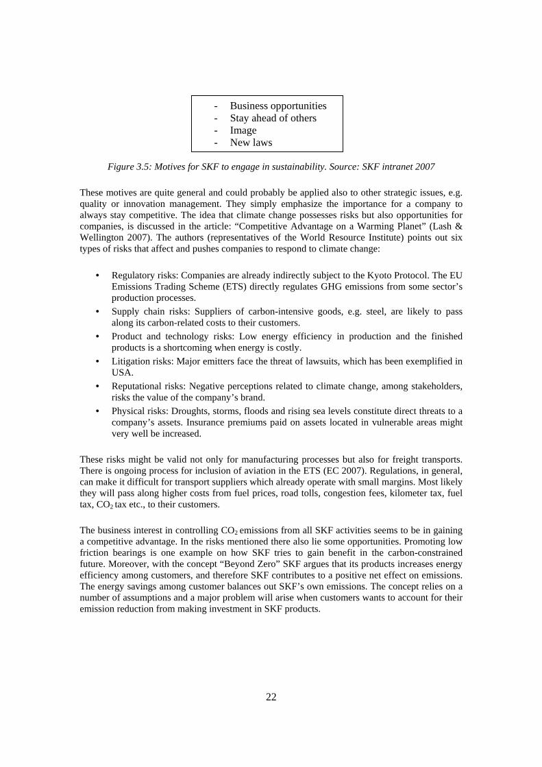
Figure 3.5: Motives for SKF to engage in sustainability. Source: SKF intranet 2007

These motives are quite general and could probably be applied also to other strategic issues, e.g. quality or innovation management. They simply emphasize the importance for a company to always stay competitive. The idea that climate change possesses risks but also opportunities for companies, is discussed in the article: “Competitive Advantage on a Warming Planet” (Lash & Wellington 2007). The authors (representatives of the World Resource Institute) points out six types of risks that affect and pushes companies to respond to climate change:

• Regulatory risks: Companies are already indirectly subject to the Kyoto Protocol. The EU Emissions Trading Scheme (ETS) directly regulates GHG emissions from some sector’s production processes.

• Supply chain risks: Suppliers of carbon-intensive goods, e.g. steel, are likely to pass along its carbon-related costs to their customers.

• Product and technology risks: Low energy efficiency in production and the finished products is a shortcoming when energy is costly.

• Litigation risks: Major emitters face the threat of lawsuits, which has been exemplified in USA.

• Reputational risks: Negative perceptions related to climate change, among stakeholders, risks the value of the company’s brand.

• Physical risks: Droughts, storms, floods and rising sea levels constitute direct threats to a company’s assets. Insurance premiums paid on assets located in vulnerable areas might very well be increased.

These risks might be valid not only for manufacturing processes but also for freight transports. There is ongoing process for inclusion of aviation in the ETS (EC 2007). Regulations, in general, can make it difficult for transport suppliers which already operate with small margins. Most likely they will pass along higher costs from fuel prices, road tolls, congestion fees, kilometer tax, fuel tax, CO2 tax etc., to their customers. The business interest in controlling CO2 emissions from all SKF activities seems to be in gaining a competitive advantage. In the risks mentioned there also lie some opportunities. Promoting low friction bearings is one example on how SKF tries to gain benefit in the carbon-constrained future. Moreover, with the concept “Beyond Zero” SKF argues that its products increases energy efficiency among customers, and therefore SKF contributes to a positive net effect on emissions. The energy savings among customer balances out SKF’s own emissions. The concept relies on a number of assumptions and a major problem will arise when customers wants to account for their emission reduction from making investment in SKF products.

- Business opportunities - Stay ahead of others - Image - New laws

23

Another way to be competitive is by setting and achieving CO2 reduction targets (SKF Annual report 2006). In this regard it is important to point out that in order to manage it is necessary to measure. A company needs to first understand the sources and the levels of its emissions (Lash & Wellington 2007). After tracking them over time the risks and opportunities can be reviewed.

3.2.2 Who should we tell? The results from the accounting process could be used in a number of different ways, and the level of accuracy may vary depending on the intended use of the information. “When defining the quality requirements it is important to carefully consider both current and future needs and consider the strategic objectives or goals that the information is intended to support” (Pålsson 2006). It can hence be important to identify the needs of the information users before the accounting procedure is decided on. If transport emissions are to be published in the annual report together with the emissions from the other sources, the figures have to be accurate. Stakeholders might respond to and question the figures, which SKF then will have to stand up for. Furthermore, any CO2 reduction target will of course be directly dependent on the baseline level, why confidence in the figures is crucial. A miscalculation from one year to the next might ruin a target with negative consequences on trustworthiness in the commitment to sustainability. A high degree of accuracy is also necessary if SKF is aiming to further concretize “Beyond Zero” by supporting the concept with actual figures. The same goes for the case if SKF is aiming for so called carbon neutrality by investing in carbon offsets to balance the own emissions. If emission figures are only to be used internally the accuracy becomes somewhat less important, because the liability is not an issue. One reason for not publishing emission figures externally is that transport emission accounting today is somewhat subjective in terms of which transports to include. Since external reporting often lacks transparency, it can be difficult to compare companies’ performance. CO2 emissions from freight transports can be a large share of one company’s accounting but a small share of another’s, even though the actual share of transports is similar. A company who chooses to include a large share of all transports might therefore appear to perform worse than a company who only includes a smaller share. Another reason to not publish emissions externally is to avoid including these emissions in the overall reduction targets. Stationary sources are, in most cases, directly controlled by the company and reduction targets can closely be followed and implemented by e.g. investing in better technology. Transport emissions might be more difficult to reduce without affecting the service to the customers since there are few sustainable transport options available.

24

3.3 Action Plan The background and the strategy have been discussed in the previous sections. The next step is to make an action plan, see figure 3.6. The two questions in this section are closely linked and will therefore be discussed in an integrated form.

Figure 3.6: Planning stage, focusing on the action plan.

Since an increasing number of companies believe that greenhouse gas accounting is important, standards have been developed to facilitate the accounting and reporting of such emissions. This is especially important for large companies with many production sites and different ownership structures. To draw company boundaries and make clear routines on how to report and which method to use is important in order to get reliable answers from all parts of the company. One of the most common standards within greenhouse gas accounting and reporting is the Greenhouse Gas Protocol. This is the standard SKF has been using so far for their greenhouse gas monitoring. The Greenhouse Gas Protocol is a partnership between the World Resources Institute and the World Business Council for Sustainable Development. The goal is to “develop internationally-accepted accounting and reporting standards for companies and other entities to report their GHG emissions” (GHG Protocol 2007). ISO also presents a standard for accounting and reporting of GHG emissions; ISO14064. For a company already committing to other ISO standards, the ISO standard on GHG reporting might seem preferable. However, the ISO14064 is directly based on the GHG protocol, and therefore there are only few differences between the two (Spannagle 2004). The result from this study is supposed to serve as the basis for discussion about calculations of greenhouse gas emissions from freight transports at SKF. Since SKF is currently using GHG Protocol, this report will follow the GHG Protocol procedure. This is only used as a frame for the discussion about the general procedure and is not exclusive. Similar working procedure is described in e.g. GRI5, ISO14064 and DANTES6. In the following sections the steps in figure 3.7 5 GRI; Global Reporting Initiative, an organization which has developed a commonly used sustainability

reporting framework. 6 DANTES; an acronym for Demonstrate and Assess New Tools for Environmental Sustainability, a

project financed by the EU.

25

will be described as well as the choices one needs to make within each of the steps. This will work as the stepping stone for the case studies in which the choices made will be analyzed in quantitative and qualitative terms.

Figure 3.7: The Greenhouse Gas Protocol procedure. Source: GHG Protocol 2007

3.3.1 Identify sources In the GHG Protocol the environmental impact is divided into three scopes. Scope 1 includes direct emissions from sources owned or controlled by the company. In Scope 2 the indirect emissions from electricity and heat production are included. These two scopes are currently covered by SKF, as mentioned earlier. In the third scope other indirect emissions, such as transport emissions from contractor owned vehicles, could be included as well. According to the GHG Protocol working procedure, scope 3 is optional7 and therefore a company could choose to not report on any indirect emissions or to choose one or several areas to focus on. Hence the guideline leave room for the individual companies to make their own choices on the level of responsibility they wish to take. The scopes are designed so that no double counting of emissions should occur for scope 1 and 2 between companies. Only one company should be able to account for emissions within the same scope. However, for scope 3 double counting might occur. The GHG Protocol gives no direct guidance on how to set boundaries for scope 3, and for transports double counting is probably rather common. Companies often set out to include both inbound and outbound transports and if all companies in the supply chain do this the sum of transport emissions will be several times higher than the actual one. However, scope 3 is not supposed to be used to compare companies or to add up information, so double counting might not be a problem if the results are used in the correct way. Even though it is not crucial to avoid double counting for scope 3, operational boundaries need to be set so that all parts of an organization use the same accounting procedure. For the case of SKF, transports are clearly a scope 3 emission since SKF itself does not own any transport carriers. However, it needs to be decided which of the company related transports that should be included in the responsibility of the company.

7 The entire concept of GHG accounting is voluntary. However, scope 3 is optional in the sense that it is

not required in order to report a GHG inventory in accordance with the GHG Protocol Corporate Standard.

1. Identify Sources 2. Select Calculation Approach 3. Collect Data 4. Apply Calculation Tools 5. Roll-up Data to Corporate Level

26

For facilities the organizational boundaries will decide to which extent the company account for emissions. The responsibility of the emissions associated with the facility can be divided according to two approaches: equity share or control approach. For the equity share a company accounts for greenhouse gas emissions according to its equity in the operation and it thus reflects the economic interest. In the control approach the company chooses to account for the emissions from the processes of which they are in control of, either operationally or financially. The control approach is used for SKF’s current greenhouse gas accounting. These above mentioned approaches cannot directly be transferred to a process such as transports since the legal terms do not quite apply, but a similar thinking might be useful. Below are a few examples of how boundaries can be set for transport emissions followed by a discussion of the advantages and disadvantages for each option. Option 1; SKF only includes the transports that SKF buys from SLS, i.e. external goods will not be included in SKF’s accounting.

• Advantages: o This excludes the emissions that external customers to SLS create. o It will avoid double counting o Relatively easy to gather the information needed.

• Disadvantages: o Does not reveal the total impact of the company activities. o Emissions can easily be lowered by changing terms of delivery. A

delivery currently carried out by SLS could be changed into another Inco term8, e.g. ex-works or FOB where the customer takes care of the transport instead, entirely or partly.

Option 2; SKF includes all transports that SLS buys from transport companies, i.e. also external goods will be included in SKF’s accounting.

• Advantages: o This option reflects the reality of the total SLS business better than

option 1. Since SKF AB owns SLS to 100 percent, SKF have full control over SLS. It can hence be claimed that SKF should be completely responsible for the emissions that their daughter company creates, since they also can take part of the financial benefits with SLS having more customers.

o Relatively easy to gather the information needed.

• Disadvantages: o Double counting will occur if the external customers would like to

account for their share of the transport emissions. o Emissions can easily be lowered by changing terms of delivery.

8 Inco terms; Standard trade definitions related to the rights and obligations of the parties to the contract.

27

Option 3; SKF includes transports in both upstream and downstream supply chain. For SKF this would mean the transports from the suppliers to the factories and the transports from the factories to the customer no matter who is the actual buyer of the transport.

• Advantages: o Reflects a vision to take responsibility for SKF’s total environmental

impact which could be beneficial in stakeholder relations. o SKF can indirectly control the inbound transports by either choosing

suppliers placed close to the production facilities, making the transport distance shorter, or by placing demands on the suppliers to choose more environmentally friendly transports.

• Disadvantages: o Transports not purchased by a SKF unit, e.g. most inbound transports

and some outbound transports where the customers handles the transport, are difficult to get information about. It might therefore be both difficult and time consuming to cover all transports.

o Administration within the company can be difficult since it is not necessarily the same company or part of the group that handles both inbound and outbound transports.

o Double counting will most likely occur since the supplier might want to account for the transports he/she buys.

o It might be difficult to set uniform boundaries on which transports to include. If inbound transports should be included, maybe also the previous transports in the early supply chain should be included.

Today there is no general rule on which approach to use, even though it could be argued that only outbound transports should be included since it makes the division of responsibility between supplier and customer more distinct (Bäckström 2007). No matter which approach used, it is of importance that the boundary is clearly stated so that the accounting is done in the same way throughout the company. Clear boundaries are also needed to make comparisons of emissions over time.

3.3.2 Select Calculation Approach There are basically two ways of calculating emissions from road transport; calculations based directly on fuel consumption or calculations based on transport activity (IFEU 2005). The alternatives can be seen in figure 3.8. In the fuel consumption alternative, the fuel consumed for the transport in question can simply be multiplied by an emission factor for the fuel (kg CO2/l of fuel) as in 1) below. This method is preferable since few assumptions need to be made, especially if only unregulated emissions are considered since chemical balance can be used to calculate the emission factor (see section 2.3.1). However, the exact fuel use can be rather difficult to collect for transport buying companies.

28

Figure 3.8: Calculation approaches. In the method based on transport activity, e.g. tonne-km or vehicle-km, more approximations need to be made but on the other hand the information about transport activity is usually easier to collect. The data needed to calculate tonne-km is, in the simplest case, the weight and distance of the transported goods as in 4) above. There are plenty of default values for emissions per tonne-km that can be applied. However, important to remember is that these default values are based on specific fill rates. To get an accurate result the specific fill rate for the actual transport should be used as in 3). Since transport activity often is chosen as a performance indicator for transports, it is important to understand the underlying mechanisms behind them. Tonne-km is often used but it is a somewhat tricky parameter. A changed number of tonne-km is not necessarily going to change the actual emissions of CO2. Improved fill rates can for example increase the number of tonnes on each vehicle, and hence the number of tonne-km, without changing the emissions. To instead base the calculations on vehicle-km reflect the reality better when the transport is done by dedicated vehicles. In this method the number of vehicles rather than the amount of goods is taken into consideration, as shown in 2).

3.3.3 Collect Data and Choose Emission Factors In this section, the input data needed to perform the calculations will be discussed. 3.3.3.1 Background to default data For exact emission data, it would be preferable to directly monitor the emissions for each transport by measurement equipment on each cargo carrier. This type of measurements does exist, e.g. on some of the large seagoing vessels. For road vehicles, measurement of fuel consumption by technical equipment is rather common. However, for large transport systems, it is difficult to use situation specific information for each transport. Even though the supplier might have quite specific data, it can be difficult to aggregate and pass on the information to the transport buyers. For mapping an entire transport system, it is therefore common to use default values instead of specific data. This will give a less accurate result, but facilitates the accounting

Calculation approaches 1. Fuel based: (Liter of fuel) x (kg CO2/ liter of fuel) = kg CO2

2. Vehicle-km based: (Number of vehicles) x (km one way) x (l of fuel/km) x (kg CO2/l of fuel) = kg CO2 3. Tonne-km based: (l of fuel/km) x (kg CO2/l of fuel) * (tonne-km) / [(Cargo capacity of the transport) x (fill rate)] = kg CO2 4. Tonne-km based - simple case: (tonne-km) x (default value for kg CO2/tonne-km) = kg CO2

29

process considerably. A general rule is to find situation-specific data to the extent possible and then use default data when needed (NTM 2007). Emission factors Carbon dioxide emissions from transports can be divided into immediate emissions from the tailpipe during the actual use of the vehicle and the more indirect emissions from other parts of the lifecycle of the transport system. The tailpipe emissions of carbon dioxide can be calculated from the direct chemical relationship as shown in section 2.3.1. The indirect emissions include emissions created during the extraction, refinement and transportation of the fuel itself. Also the capital goods, i.e. manufacturing of vehicles, building of roads, maintenance of vehicles etc. can be included. A lifecycle perspective ensures that no part of the environmental load of the process is neglected (Blinge et al. 1998). It becomes specifically important when accounting for transport modes with different propulsion e.g. electrical rail and road transports, or different types of fuels, e.g. diesel and ethanol. In the case of diesel, the indirect CO2 emissions from heavy duty vehicles can be estimated to about 5-15 percent of the direct emissions from the fuel (IVL 2001, IFEU 2005). Figure 3.9 shows the relative energy consumption from different stages of the diesel fuel production. A comparison is made to electricity production9, where the end use contributes to a comparatively small share of the total. This indicates why a lifecycle perspective can be important when comparing transport modes.

Figure 3.9: Energy consumption for diesel and electricity. Source: IFEU 2005.

9 The allocation of energy consumption to the different phases is dependent on the type of electricity

production. An energy efficiency of 30-40 percent, as in figure 3.9, is normal for e.g. coal-fired power plants.

30

Capital goods, i.e. manufacturing and maintenance of vehicles, roads, rail etc, is more difficult to include. Most studies do not include them for reasons of feasibility (Baumann and Tillman 2004) and this is also the reason why it is not included in this study. However, a recent study shows that capital goods could contribute to around 18 percent of freight transport’s total emissions of greenhouse gases (Frischknecht et al. 2007). Fuel and electricity consumption For road transports, it is difficult to calculate or measure the exact fuel consumption for each single vehicle and engine type. To make it easier, the vehicles are divided into different categories. Each category of vehicles can then be assumed to have the same fuel consumption. The fuel consumption will of course differ depending on a variety of reasons and is not only depending on the size of the vehicle. Some of the most contributing factors are discussed below. These factors are normally included in the default values, which are thought to describe the “normal” driving condition.

• Road category: Urban, rural or highway driving will affect the fuel consumption and the amount of regulated emissions. Urban driving normally requires more fuel per km since there are more starts and stops and more idling.

• Vehicle load: The load is often a large part of the total weight for heavy duty vehicles and has a substantial influence on the fuel consumption. The relationship can be assumed to be linear, with a 30 percent difference in fuel consumption between an empty and a full truck (NTM 2007).

• Gradient: Flat, hilly or mountainous landscape will affect the fuel consumption in different ways. The fuel consumption for driving in a hilly landscape can be estimated to ten percent higher than driving in a flat landscape (IFEU 2005).

• Driving conditions: The fuel consumption varies depending on vehicle speed. To get a realistic value, the different speeds during a distance should be taken into consideration. However, this is not always feasible and average speed can be used instead, with a somewhat less accurate result. Another impact on the result is the driver’s behavior when driving. Eco driving, i.e. driving in a more fuel saving manner, can reduce fuel consumption with around 10 percent (Swedish Road Administration, 2007).

• Tire pressure; Low pressure in the tires can increase fuel consumption with about two percent (NTM 2005).

Estimations of carbon dioxide emissions from sea transports are more difficult than for road transports, since each vessel is built as an individual with specific characteristics. Again, the best method to find the carbon dioxide emissions would be to find out the specific fuel consumption for the transport, but since this can be difficult general numbers often have to be used. Vessels are often categorized into following groups; ferries, general cargo vessels (RoRo, LoLo and container ships), bulk cargo vessels and tankers (IFEU 2005). Each group can be allotted an energy consumption factor which is multiplied with an emission factor for the fuel to get the final emissions. However, the calculations for sea transports can differ significantly depending on the carrier classification and the choice of allocation methods. The fuel consumption will of course also be dependent on e.g. weather conditions, waves and currents.

31

For railway the transports can be carried out by either electricity or diesel trains. For electrified railway the electricity production is important to include. The energy consumption will vary depending on e.g. the gross weight of the train set, the length of the train, and the gradient of the tracks. A division depending on cargo type can also be made, e.g. bulk, average and volume goods (EcoTransIT 2007). Air transportation can be calculated by differentiating the takeoff/landing part from the cruising part (NTM 2007). The cruising emissions will depend on the distance and the takeoff/landing emissions will be constant no matter the flight distance. Allocation Allocation is a crucial parameter for all transport modes and it will significantly contribute to the results. In default values, such as g CO2/tonne-km, specific allocation decisions are often implied. In order to make a calculation as accurate as possible, it is therefore important to be aware of the assumptions behind the default values since they might not be relevant for the situation specific case. There are a variety of different ways allocations can be made, and no strict rules are established (Bäckström 2007). Different transport modes or situations might require different allocation methods. However, one thing to remember no matter allocation method; all emissions should be dedicated to the cargo itself, not to the cargo carriers (NTM 2007). Physical measurements, like weight or volume, are commonly used and the choice of which one to use is preferably made based on the limiting factor of the transport; if the transported goods are heavy, the weight will set the limit and hence allocation based on weight is the most logical choice. However, it can get tricky when both volume and weight goods are transported on the same transport. In those cases, a translation factor can be used to relate volume and weight goods. In Europe a general calculation rule for road transports is that one cubic meter corresponds to 333 kg (Schenker 2007). If using a translation factor, the fill rate can thus exceed 100 percent. Lane meter allocation is another method which is commonly used for RoRo vessels, since this is the limiting factor. For container vessels, e.g. TEU10 can be used. For ferries carrying cargo and passengers, the allocation might not be as straightforward since the limiting factor can be indistinct. One option is to allocate based on the number of decks, and then allocate the emissions per deck on the weight or lane meters (Bäckström 2007). Another question concerning allocation of goods is how the positioning of the cargo carrier should be included. To include positioning implies that the buyer of the transport should be responsible not only for the purchased transport from pick-up to delivery location but also for the transport of the cargo carrier to the pick-up location. Often the carrier performing the transport is not located at the pick-up location at the time the transport is ordered, but needs to go to the pick-up location empty or with only a smaller load. However, it is generally difficult for the customer to know what happens before the carrier arrives to the pick-up location. One solution is to ask the supplier for the data on filling rate for the transport to the pick-up location. Another solution, which can be significantly easier, is to add 50 percent of the total distance of the bought transport (NTM 2007). This number is based on the

10 TEU= twenty foot equivalent unit (the space that a standard 20 foot container occupies)

32

assumption that the transport to the pick-up location has a fill rate of 50 percent and hence the transport buyer should take responsibility for the empty half of the positioning distance. Whether to include positioning distance or not, is in the end a question about responsibility. Since the transport buyer has no control of these transports, they have no possibility to directly influence or improve the positioning part of the transport. For SKF, where fill rates have been highly prioritized, an addition of 50 percent to the emissions only due to positioning would not show the true efficiency of the SKF dedicated network. It could be argued that the transport suppliers are responsible for choosing customers in a way that optimizes their total transport system (Lumsden 1998). However, there are some basic inequalities in the transport system for which the transporters cannot be held responsible. Some countries export more than they import, and thus the problem is deeply rooted and cannot be handled by individual forwarders or haulers. But the system inequality is not the only reason for the inefficiency of the transport system. On average, one out of four trucks drives empty (Blinge, in Chalmers Magasin, 3/4 , 2006, p.10) .The solution to this problem is probably not to blame either the transport buyer or the supplier, but rather open up for discussion on how the problem could be solved. The question of positioning distance will not be discussed further, but could be kept in mind for future discussions between SKF and their forwarders. Better forecasts on the transport demand might help the forwarders to increase the overall efficiency. For dedicated vehicles the allocation procedure can be excluded since the emissions of CO2

basically only will depend on the total weight, the vehicle type and the engine power. The number of vehicles is the more important issue to base the calculations on and therefore no allocation problem arise apart from the positioning question. For non-dedicated transports, the optimal solution is if the transport supplier provides data on filling rate. This can however be sensitive information since it can reveal the company strategy. In such case, default filling rates can be used. As an example European road transports can be assumed to have a fill rate of 70 percent (NTM 2007). Vehicle operation distance The vehicle operation distance is an important factor in the calculation of transport emissions. However, to find out the exact distance for every transport can be difficult and time consuming. Seen from the transport buyer’s perspective, the distance can be estimated by internet tools, e.g. ViaMichelin, but it is difficult to know if this value corresponds to the actual distance. In dedicated networks in which a company buys the whole cargo unit from the supplier, it is generally easier to make assumptions since the cargo will be transported according to the transport agreement. For non-dedicated transports, it can be a lot more complicated. Transport suppliers often use consolidation of goods as a means of increasing the efficiency in the overall transport chain. The customer’s goods could be transported via a consolidation point that will make the total distance significantly longer than the shortest distance between the pickup location and final delivery location. This parameter can be difficult for the customer to take into consideration, especially for non-frequent transports. The best solution would be if the vehicle operation distance could be provided by the supplier, but if this information is not available estimations need to be done. Methods on how to handle distance for non-dedicated transports have been described by e.g. NTM (2007).

33

Level of detail For the four input data categories discussed so far, a choice has to be made on how detailed the input data should be. A transport calculation can be made simple or complicated, depending on the needs of the information user. A trustworthy result is important, but the concept of trustworthiness is somewhat subjective. A choice has to be made on what is a “good enough” result. This depends on the intended use of the result, as discussed in section 3.3.2. If it is only voluntary accounting the result does not need to be as exact as it needs to be when used for regulative purposes. Depending on where in the logistics chain the company is placed, the possibility to get exact results differs. A hauler is in direct control of the transport and could therefore provide very detailed information about distances and fuel usage for each transport. The forwarder might be able to receive the exact data from the hauler, but aggregated data is probably more convenient to handle. For the transport buyer it might be difficult to handle each transport separately, even though this data might be provided, and some generalizations might be needed due to the complexity of the transport systems. Also, for transport buying companies, the collection and interpretation of data cannot be too demanding in time and resources.

3.3.3.2 Collection and quality of data In the existing standards, e.g. the ISO14000 series, there are requirements on data quality but little or no guidance on how to practically perform data collection to ensure data quality (Pålsson 2006). This makes it difficult both to compare and verify results and is therefore a main problem in the attempts to measure transport emissions (Swahn 2007). The collection of data for transport emissions for a transport buying company can basically be performed in two ways; relying on transport information from the own organization or asking the contracted transport suppliers for it. If the transport suppliers are asked for information, it must be decided which level of information the company wishes to receive. One can, e.g., ask for the total greenhouse gas emissions and let the supplier do all the calculations. The total emissions are then just the addition of the numbers received from the suppliers. One can also choose to only collect raw data on transport activity, e.g. number of trucks, distance and fuel consumption, and perform the calculations within the company. As stated earlier, situation specific data should be used if possible (NTM 2007). Logically, the transport company should be able to provide more situation specific information, but in reality this can be difficult even for the provider of the service. The pros and cons with the different data collection methods will be discussed in chapter 4 where a transport system is mapped. The quality of the data will also be addressed.

3.3.4 Apply Calculation Tools There are several different calculation tools that can be used for greenhouse gas accounting. When following the GHG Protocol standard, the tool used is not so important. There is a recommendation to use the GHG Protocol’s own tools, but this is optional. GHG Protocol’s specific tool for mobile combustion is very general which makes it easy to use but on company level it might not be the most convenient method. A company could easily develop an individual tool that better suits their specific needs.

34

It is also common that companies already have some type of database in which environmental information is handled. It could be beneficial to include all emissions in the same system. Such a system will decrease the overall costs since the accounting process will be better structured. It will also ensure better quality of the environmental information since all calculations will be based on the same set of data. (IVL 2002)

3.3.5 Roll-up Data to Corporate Level In the GHG Protocol there are two basic approaches to handle the accounting of emissions within a company; the centralized approach and the decentralized approach. In the centralized approach, activity data is collected from each site and the actual calculations are carried out on corporate level. In the decentralized approach each site makes their own calculation and only reports the total emissions to the corporate level. A benefit with the centralized approach is that the responsible person often has more knowledge in the environmental field. However, on the decentralized level the staff might be more aware of the actual situation at the specific site. Important, especially for the decentralized approach, is that a general, companywide, guideline exist to ensure consistency (Erlandsson 2006).

35

4. Mapping a logistics system This chapter is devoted to the do-phase, see figure 4.1, and hence CO2 emission calculations based on the discussed methodology will be performed for a delimited transport system.

Figure 4.1: The do-phase, with focus on implementation of the plan.

4.1 System description In the 1980s SKF’s European distribution structure differed compared to today’s set up. There were 18 local and seven international factory warehouses, located close to production sites (Toepfer 2007). The transports between warehouses were based on deliveries with full trucks, which often caused long lead-times for some products, since trucks waited on the pick-up location until fully loaded. Hence the system could not meet up with customer’s requirements for short lead-times, which led to the discussion of reshaping it into the so-called New European Distribution Structure (NEDS). (Axelsson and Dahlqvist 1999). A crucial sub-component of NEDS was the Daily Transport System (DTS) which organizes the European logistics activities for outbound transports, i.e. transportation of finished products to final customers. DTS became operational 1992 and proved to be successful considering all objectives were fulfilled, i.e. improved delivery service to customers, reduced inventories and reduced distribution costs (Axelsson and Dahlqvist 1999). The nowadays mature DTS relies on the strategic cornerstones listed in figure 4.2.

36

Figure 4.2: The DTS logistics strategy. Source: SKF intranet 2007 The DTS distribution structure includes transports between a number of international and domestic hubs (terminals) that connect SKF production sites with the customer markets. The system is being demonstrated in figure 4.3.

Figure 4.3: The Daily Transport System. The picture is somewhat incomplete since

a number of production sites are not shown. Source: SKF intranet 2007 The European Distribution Centre (EDC) is the regional warehouse for Europe. It is located in Tongeren (Belgium) which belongs to a European core area with a high level of ground transport infrastructure and some major airports and harbors (Nijkamp et al. 1998). With a great storing capacity and a large number of order lines (5 000 000 annually) the EDC has the main task to

The DTS logistics strategy: • Dedicated and reliable service: dedicated traffic gives attention to

reliability and speed. • Cost effective concept: cross-docking at hub, giving shorter lead-

times, lower costs and better frequency. • Fixed timetables: departures and arrivals including hub-operations are

scheduled. • Daily deliveries: most markets are served daily. • Door to door service: goods are delivered from gateway to customer. • Short lead-times: 48 (72) hours across Europe.

37

serve the aftermarket, consisting of a large number of customers ordering smaller quantities (SKF intranet 2007). Examples of such customers are retailers and car repair shops (Olsson 2007). The DTS also contains four so-called Logistics Service Centers (LSC) located in Gothenburg (Sweden), Schweinfurt (Germany), St Cyr (France) and Airasca (Italy). These warehouses are all positioned close to production sites and thus each LSC have responsibility for consolidating goods from specific factories. Compared to the EDC, the number of order lines at the LSC are much less (around 300 000- 500 000 per year) (SKF intranet 2007). However, since most customers are original equipment manufacturers, that make fewer but larger orders, the annual shipping volumes are in general larger from the LSC compared to the EDC. Apart from the hub at EDC and the hubs at the four LSC there are two international hubs located in Helsinki (Finland) and Vienna (Austria). These, however, are not operated by SLS but are outsourced to another third party logistics supplier. All hubs function as goods consolidation and deconsolidation points. The goods are cross-docked, which means it is instantly reloaded from incoming to outgoing trucks. This of course delimits the need for building up stocks (Lumsden 1999), and consequently hubs are not considered to be warehouses. There are also around 30 domestic hubs in Europe which fill the purpose of serving the customers in the country of location. These hubs are not included in the DTS and neither are they operated by SLS but by other third-party logistics providers. The delimitation of DTS is further explained by figure 4.4 which illustrates the various ways that goods can be transported from factories to customers. DTS is captured within the shaded area. Hence transports from factories to international hubs as well as distribution from domestic hubs to customer, Freight to Customer (FTC), are not included in the DTS. Within the DTS the specific goods can be transported to and from international hubs but always exit the system in a domestic hub to become a FTC reaching the final customer. Production site/ Factory warehouse Int. hub Int. hub Int. hub Dom. hub Customer

Figure 4.4: Distribution of goods from a SKF production site to a customer.

The shaded area sets the DTS system boundary.

Every hub within the DTS is physically connected by the flow of goods which completely relies on road transports, purchased from about 30 different forwarders. The trucks can be either Full Truck Load (FTL) or Less than Truck Load (LTL). FTL trucks are fully dedicated, i.e. they only carry goods for SLS and operate according to the strict DTS timetable thereby going direct from hub to hub. LTL are used for smaller shipments where SLS buys a share of the truck’s loading capacity. By necessity this goods need to be adapted to the overall transport assignment of the forwarder. Ferry transports are used when necessary e.g. between Scandinavia and the continent or for crossing the Baltic Sea.

38

Being a part of a global logistics system the DTS is more or less linked to other transportation networks organized by SLS or its business partners. These are:

• Freight to customer: distribution of goods from domestic hubs to customer.

• Global air freight program: air freight serving world markets with a 72 hour lead time.

• Global sea freight program: ocean going vessels serving world markets on a weekly time schedule.

• Regional transport systems: the equivalence of DTS operating in other regions. SKF serves customers in 170 countries world-wide.

• Supply chain transports: material supporting transports going from suppliers to SKF production sites, between SKF production sites, and of course from production sites to hubs.

4.2 Assumptions In order to map the CO2 contribution from the DTS, a number of assumptions have to be made. These are explained in the following section.

4.2.1 Method The emissions from SKF’s goods transports clearly falls under scope 3 in the GHG Protocol approach since all transports are carried out by contractor owned vehicles, either owned by the forwarder or its sub-contracted hauler. For this case only the outbound flow of finished products is included and the specific focus is on the DTS. The emission factors are based on NTM, Network for Transport and Environment, which is a Swedish network with the aim of creating a common guideline for how the emissions from transports should be measured. NTM is not itself performing any scientific studies on transport emissions. Instead they update the data according to what they consider the best available data at the moment (NTM 2007). Right now the data for road transport is based on the HBEFA11 report, which was made in collaborations between authorities in Germany, Austria and Switzerland. The data will be updated according to the ARTEMIS project when the report from this project is released. ARTEMIS is a project within the European Union with the goal of creating a common guideline for transport emission calculation within Europe, and therefore has a good chance of becoming the standard for emission calculations both in Sweden and the rest of Europe. This choice of default data will exclude unburned carbon and neither will it include a lifecycle perspective. Since other greenhouse gases from transports have a minor contribution, only carbon dioxide is included. The emissions are calculated in an excel sheet designed for this specific study. The method behind the calculations is based on both the GHG Protocol and NTM with the emission factors adopted from NTM.

11 HBEFA = Handbook of emission factors for road transport

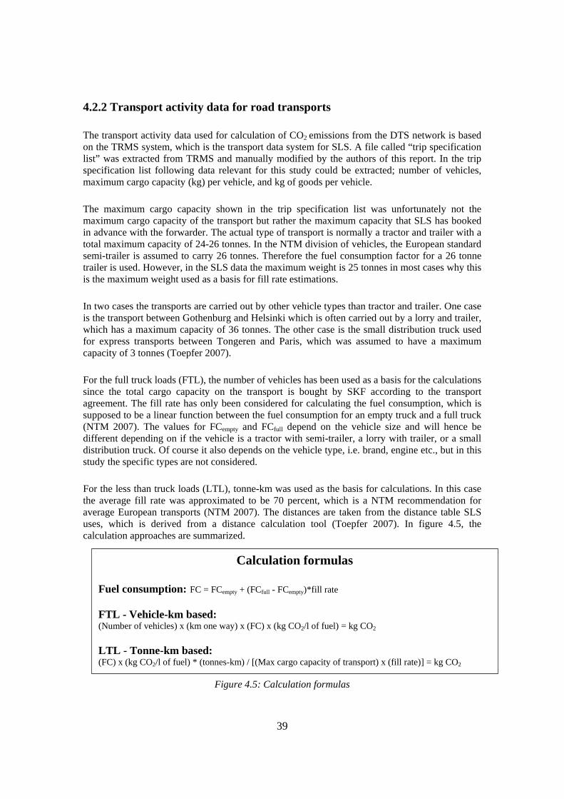
39

4.2.2 Transport activity data for road transports The transport activity data used for calculation of CO2 emissions from the DTS network is based on the TRMS system, which is the transport data system for SLS. A file called “trip specification list” was extracted from TRMS and manually modified by the authors of this report. In the trip specification list following data relevant for this study could be extracted; number of vehicles, maximum cargo capacity (kg) per vehicle, and kg of goods per vehicle. The maximum cargo capacity shown in the trip specification list was unfortunately not the maximum cargo capacity of the transport but rather the maximum capacity that SLS has booked in advance with the forwarder. The actual type of transport is normally a tractor and trailer with a total maximum capacity of 24-26 tonnes. In the NTM division of vehicles, the European standard semi-trailer is assumed to carry 26 tonnes. Therefore the fuel consumption factor for a 26 tonne trailer is used. However, in the SLS data the maximum weight is 25 tonnes in most cases why this is the maximum weight used as a basis for fill rate estimations. In two cases the transports are carried out by other vehicle types than tractor and trailer. One case is the transport between Gothenburg and Helsinki which is often carried out by a lorry and trailer, which has a maximum capacity of 36 tonnes. The other case is the small distribution truck used for express transports between Tongeren and Paris, which was assumed to have a maximum capacity of 3 tonnes (Toepfer 2007). For the full truck loads (FTL), the number of vehicles has been used as a basis for the calculations since the total cargo capacity on the transport is bought by SKF according to the transport agreement. The fill rate has only been considered for calculating the fuel consumption, which is supposed to be a linear function between the fuel consumption for an empty truck and a full truck (NTM 2007). The values for FCempty and FCfull depend on the vehicle size and will hence be different depending on if the vehicle is a tractor with semi-trailer, a lorry with trailer, or a small distribution truck. Of course it also depends on the vehicle type, i.e. brand, engine etc., but in this study the specific types are not considered. For the less than truck loads (LTL), tonne-km was used as the basis for calculations. In this case the average fill rate was approximated to be 70 percent, which is a NTM recommendation for average European transports (NTM 2007). The distances are taken from the distance table SLS uses, which is derived from a distance calculation tool (Toepfer 2007). In figure 4.5, the calculation approaches are summarized.

Figure 4.5: Calculation formulas

Calculation formulas

Fuel consumption: FC = FCempty + (FCfull - FCempty)*fill rate FTL - Vehicle-km based: (Number of vehicles) x (km one way) x (FC) x (kg CO2/l of fuel) = kg CO2 LTL - Tonne-km based: (FC) x (kg CO2/l of fuel) * (tonnes-km) / [(Max cargo capacity of transport) x (fill rate)] = kg CO2

40

4.2.3 Transport activity data and calculation methods for other modes Three other transport modes will be discussed; short sea, air and rail. Short sea transports are a part of the DTS since some relations require it, e.g. transports from UK or Sweden. The air transports are not included in the DTS at all, but will serve as a point of reference on the relative emissions from different transport modes. The calculation method for rail transports will be used in one of the case studies discussed in section 5.1. The sea, air and rail calculations are not as detailed as for road transports. For short sea transports, the data on transport activity was based on data from the DTS distance list (number of km) and the TRMS file (number of tonnes). Data for RoRo ships was collected from DFDS Torline (Nilsson 2007). Total fuel consumption per km, average fill rate (based on lane meters), and maximum cargo capacity were given and together this resulted in 43 grams per tonne-km. For ferry transports, data was taken from the Stena Line’s homepage. Allocation was made by first dividing the emissions by the number of decks. For the freight decks the remaining emissions were allocated by lane meters according to NTM guidelines. For air freight, the data on transport activity was based on data from the air freight suppliers. The data covers the total transports within the global air freight program during the first two quarters of 2007. The distances were taken from the web site “world airport codes” (2007). In some cases the exact airport code was stated in the supplier data. However, sometimes only the departure and destination countries were stated. In those cases, one airport in the capital city was chosen for the distance calculation. For air transports, a distance for circulation before landing can be included. However, since no detailed information about the specific flights was known, this was not included. The airplane types were not known, and therefore three different planes from different size categories were chosen for the calculation. These plane types were chosen since the suppliers, on their homepages, stated that they use these types (DHL 2007, Kuehne and Nagel 2007). This does not mean that these are the actual airplanes used for the SKF transports, but gives an indication that these are commonly used planes for freight transports. The emissions are calculated according to the NTM guidelines for air freight (NTM 2007). As discussed earlier, the emissions are divided into two parts; constant emission factor (CEF) and variable emission factor (VEF). The CEF corresponds to the high fuel usage during takeoff and landing and the VEF corresponds to the fuel use during the cruising. The emission factors depend on plane type and fill rate. Since also the fill rates were unknown, two different fill rates – 50 and 75 percent – were used for each plane type. The formula for the total carbon dioxide emissions is:

Total CO2 emissions [kg] = CEF [kg] + VEF [kg/km] x distance [km] The rail transports in this study are mostly carried out in Germany (see section 5.1) by electrified rail and hence only this is discussed. The methodology is taken from EcoTransIT, which is an environmental load calculator developed by IFEU in corporation with several rail companies in Europe (IFEU 2005). This electricity consumption is assumed to be dependent on the weight of the train set and the gradient of the tracks. The emissions from the electricity consumption are based on the national electricity mix in each country or, when data is available, the specific electricity for the rail transports. These details are listed in IFEU (2005).

41

4.3 Results

4.3.1 Daily Transport System The total emissions of CO2 for the DTS system week 1-26 2007 were 4 837 tonnes of which 4 408 tonnes originated from the FTL transports and 428 tonnes from the LTL transports. For one year the emissions are approximately twice of this, i.e. 9 674 tonnes. It is not an obvious approximation that the emissions for the last two quarters will be the same as for the first two quarters. Hence the number for the whole year should be seen merely as an assumption. However, for 2006, the first two quarters represented 51 percent of the total amount of goods transported during that year (SKF intranet 2007), which supports the assumption. Figure 4.6 shows the distribution of emissions for the FTL relations. A description of the relations can be found in appendices 6 and 7.

Figure 4.6: Distribution of emissions between the FTL relations.

This result might be misleading since relations such as GOTG (Gothenburg-Tongeren) and GOSW (Gothenburg- Schweinfurt) have large total emissions when they in fact are the most efficient relations in regards of fill rate. To illustrate the efficiency of each relation the amount of CO2 per tonne-km is shown in figure 4.7. The relations starting from Gothenburg have the highest fill rates and thus the lowest emissions per tonne-km. The extreme relation Tongeren – Paris express (TGPX) has the highest amount of emissions per tonne-km, 0.34 kg CO2, due to the use of a small sized vehicles and low fill rates. This is approximately ten times higher than the most efficient relations.

42

Table 4.7: Kg of CO2 per tonne-km for each FTL relation.

For LTL the results for each relation are shown in table 4.8. As can be seen, the relation Gothenburg-Helsinki (GOHE) is by far the largest contributor and due to the large volumes on this relation, it has recently been changed into a dedicated flow. The amount of emissions per tonne-km will be the same for all relations; 48 grams. This is a direct result of the assumed fill rate of 70 percent on all LTL relations.

Figure 4.8: Distribution of emissions between the LTL relations.

The sea transports included in the DTS system contribute to about two percent of the total DTS emissions of carbon dioxide. Since the sea transports are carried out by fast vessels that are relatively small, the emissions per tonne-km were in most cases higher for the sea transport than for the road transport.

4.3.2 DTS compared to air freight In figure 4.9 the carbon dioxide emissions from the SKF global air freight program during the first two quarters 2007 are shown. The choice of plane type and fill rate has a large impact on the result. If a B747 with 75 percent fill rate is used, 13 400 tonnes will be released. If an airbus A300 with 50 percent fill rate is used 28 700 tonnes will be released. This is a very large span, but it is reasonable to conclude that the actual emissions are somewhere within this interval.

43

Figure 4.9: Emissions from air freight depending of the type of airplane and fill rate.

An average estimation could be around 20 000 tonnes, which is around four times as much as the result from the DTS calculation.

The contribution of air freight to the total transport emissions is substantial. Of the total tonnes of transported goods (within the DTS and the global air freight program), air freight only stands for three percent of the transported weight. However, out of the total carbon dioxide emissions, air freight contributes to 80 percent.

44

4.4 Analysis In this section the results from the DTS case study will be analyzed as seen in figure 4.10. First a sensitivity analysis of the calculations will be made and after that an analysis of the method choices will be discussed. In the end a discussion about data certainty and quality will be presented.

Figure 4.10: Check phase, focusing on analyzing the results.

4.4.1 Sensitivity analysis A sensitivity analysis was made on all relations for both the LTL and the FTL flows. An example of how this was made can be seen in table 4.1, where the relation Airasca to Schweinfurt (AISW) is analyzed. The table also emphasizes the calculation method used in the previous section. The analysis serves the purpose of testing how a selected variation in a few parameters will affect the final result. The parameters are; distance, fuel consumption and emission factor. The variations are based on the authors’ judgments, which in turn are influenced by the assumptions made by NTM (2007) and the indications from contacted transporters. It is estimated that the distance will differ more to an upper end than to a lower end, e.g. the figure 990 km has an estimated variation of –2 percent and +5 percent. The assumption is that the contracted distance is rationally based on the shortest possible route, and therefore it should be more difficult to make short cuts than it is to make detours. For fuel consumption, NTM suggests +30 percent in the upper fuel consumption interval, but since none of the contacted transporters were close to these numbers, ten percent was chosen as the upper and lower limit. The small variation in the emission factor comes from the marginal differences in density and carbon content of different diesel fuel blends. The result is 303 tonnes of CO2 with a minimum value of 266 and a maximum of 352 tonnes. Applied to all FTL relations, the variations are between 3 857 and 5 091 tonnes of CO2. By comparing with the final result of 4 408 tonnes, as calculated and presented in chapter 4.3.1, the analysis suggest an uncertainty of about +15 and -12 percent. Since the uncertainty is directly proportional to the multiplied variation of each parameter the fuel consumption will have the largest impact on the total uncertainty.

45

Table 4.1: Sensitivity analysis of the relation Airasca – Schweinfurt Description of transport relation Entity Unit

Transport: Airasca to Schweinfurt estimate Value low high

1. Traffic mode Truck 2. Truck type Heavy Diesel Truck 3. Truck size Tractor + semi trailer 4. Cargo [tonne] capacity (CC)

25

5. Cargo type Average heavy goods 6. Fill rate (FR) [%] FR = Weight(cargo) / CC

86,5

7. From Airasca (Italy) 8. To Schweinfurt (Germany) 9. Distance [km] 990 970 1040 10. Uncertainty in distance [%] -2% 5% 11. Number of trips (week 1-26, 2007) 343 12. Vehicle-km [v-km] Vehicle-km = number of trips * distance

339570 332710 356720

13. Fuel consumption (FC) [l/km] FC = FCempty + (FCfull - FCempty) * FR FCempty = 0,236 FCfull = 0,354

0,338 0,304 0,372

14. Variation in FC [%] -10% 10% 15. Emission factor CO2 [kg/l fuel] 2,642 2,628 2,655 16. Fuel volumetric heating value [MJ/l fuel] 35,8 17. CO2 emissions (week 1-26 2007) [kg] CO2 [kg] = v-km * FC * Emission factor

303235 265806 352318

18. Energy consumption (EC) – Fossil [MJ] EC [MJ] = v-km * FC * volumetric heating value

4108933 3583620 4659296

There are other uncertainties, related to the assumptions, which are not accounted for in the table. As discussed before the factor kg CO2/liter of fuel depends on the carbon content of the fuel and to what extent the unburned hydrocarbons are taken into consideration. If HC and CO are excluded, the carbon dioxide emissions will decrease with about one percent. The factor kg CO2/liter of fuel also depends on to what extent the lifecycle of the fuel or process is included. If only the life-cycle of the fuel would be included the emissions would be around five percent higher (Bäckström 2007). If the whole lifecycle of the entire transport is included (both capital goods and the fuel) the total emissions will be, on average, about 27 percent higher, based on Frischknecht (2007).

46

4.4.2 Analysis of method choices Not only the variation of input data in terms of fuel consumption, distance etc. influences the results. In this section, the assumptions behind the model used will be discussed. To make it easier to follow, the same structure as previously used, i.e. the GHG Protocol procedure will be applied.

4.4.2.1 Step 1; Identification of sources – changing boundaries In the DTS case the external goods were included and hence the approach to include all transports SLS purchases was used. In this section a change of the boundaries will be made in order to see how the inclusion or exclusion of external goods will affect the incentives for energy reducing activities from transports within the SKF group. Today, it can be argued that the external customers generally do not imply more transports since the external goods only fill up the already existing dedicated trucks, and hence only improves the overall fill rate (Karlsson 2007). However, with a strategy to increase the number of external customers, it might be difficult to continue to increase the fill rate and presumably more transports need to be used. Three different scenarios will be discussed. In the “base year” it is assumed that ten percent of the goods in weight are external, which is the situation today (Ohlsson 2007). The short sea transports are not considered and neither is the fill rate’s impact on fuel consumption, i.e. the fuel consumption is constant. Scenario 1 – increased transport work, constant fill rates: The total amount of vehicles in the DTS increase by ten percent on each relation from today’s rate. The entire increase is made by introducing more external customers. The fill rates are kept constant. Scenario 2 - increased fill rates: The amount of external goods increases in a way so that the fill rates increase from today’s rate to 85 percent on each relation. The relations that today have more than 85 percent fill rate were kept constant. The number of trucks was also kept constant. This illustrates a situation where the external customers are actively chosen to suit the already existing DTS structure. The DTS network will hence be more efficient. Scenario 3 – decreased fill rates: The amount of external goods increases in a way so that that the fill rates decrease since the number of transports needs to be increased. This illustrates a situation where the external customers are not chosen strategically and hence the DTS system will be less efficient than before. In the first scenario, illustrated in figure 4.11, the total amount of transport work has increased. If only SKF goods are included in the accounting, the extra transport work will not show and the emissions are thus the same for both years. If external customers are included in the accounting, the emissions will increase.

47

Table 4.11: Scenario 1 where the transport work for external customers has increased.

The second scenario, figure 4.12, represents a situation where SLS has improved the fill rates by increasing the amount of external goods on the routes where the fill rate earlier was low. The emissions will not change if both external and internal goods are included. However, if only SKF is to be considered in the calculation, there is a clear decline in CO2 emissions. In this case, it will provide a good incentive to increase fill rates to only include SKF goods.

Figure 4.12: Scenario 2 - increased fill rates.

In the first two scenarios it can be of high importance to also look at other factors beside the total amount of CO2 emissions. To use the performance indicator carbon dioxide per tonne or per tonne-km could be used as a complement. If one wishes to include both internal and external customers in the calculations for scenario two, the CO2/tonne-km will be 44.2 grams for the base year and 43.8 for year 2. This can be used to show how the efficiency of the system has improved even though the amount of carbon dioxide is the same as previous year. In the third scenario, figure 4.13, an increase of external customers leads to more transported goods, an increased number of trailers and a lower fill rate. This will result in higher emissions both with and without the inclusion of external customers. However, the increase in CO2 will not be as apparent if only SKF goods are accounted for. Excluding external customers will thus “hide” the real inefficiency of the system.

48

Table 4.13: Scenario 3 – decreased fill rates.

4.4.2.2 Step 2: Calculation approach In the DTS base scenario (section 4.3), the calculation method for FTL was vehicle-km and for LTL tonne-km. This method can be made simpler by using tonne-km as a basis for calculations for the entire DTS network. A standard value of g CO2/tonne-km could be used, e.g. the recommendation 50 g per tonne-km for a tractor with semi-trailer12 (Baumann & Tillman 2004). If this method is used the total CO2 emissions for the DTS network will be 5476 tonnes, which is 13 percent higher than the more detailed calculation. To use the simplified tonne-km based approach will not only make the calculations simpler but also more consistent. The information about the dedicated transports within the DTS network is detailed, but this is only one part of the SLS transport network. The rest of the network consists of LTL vehicles and transports carried out by other modes than road. For e.g. sea transports, it is very difficult to estimate emissions and normally default values such as g/tonne-km needs to be used since there is no other method which is easy to use for large transport systems. To use tonne-km based calculations for all transports could make the overall calculation method more straight forward. According to figure 3.8, the value for grams per tonne-km can easily be adjusted to the specific case. An option could therefore be to use specific values for the dedicated networks and general numbers, such as the one used above, for the non-dedicated transports and other modes than road. However, an important aspect of the tonne-km based calculation is that the efforts of increasing fill rates of the trailers will not be noticed directly. If the transport work increases, the CO2

emissions will increase proportionally as well even if the fill rates have increased. To only use tonne-km as a measure is not giving the full picture and indicators such as g/tonne goods or g/tonne-km will also be useless. Therefore, if a company wants “credit” for improved fill rates, the default value of g/tonne-km has to be adjusted to the new fill rate for the change to break through. Since fill rates is an important measure to increase efficiency of the transport system both from a financial and an environmental perspective, it could be recommended.

12 The value 50 grams excludes the LCI emissions which are approximately 4.5 percent in the NTM

estimates (Bäckström, 2007).

49

If many different transport modes are included in the overall calculations, the indicator g CO2/tonne-km can be used to reflect changes of modes within the transport system. A change from a more energy intensive mode, e.g. road, to a less intense, e.g. rail, will then be seen since the overall g/tonne-km will be lowered. However, logically, such an indicator will be completely useless if only road transports are included, since it will be exactly the same as the input default value.

4.4.2.3 Step 3: Data collection method In section 3.3.3.2 three different ways of collecting input data was discussed. Two of them will be analyzed here; company data as used in the DTS base scenario and raw data from transport suppliers. The calculation method is the same as in the DTS base scenario but instead of using NTM and TRMS data for fuel consumption and distance, raw data from the forwarders was used. In a questionnaire the forwarders were asked to specify the fuel consumption and the driving distances (Appendix 2 and 3) for the transports carried out for SLS. The questionnaire was answered by twelve out of 22 forwarders. However, the LTL flows were difficult to draw conclusions from since the replies in many cases did not cover the questions asked, and therefore only the FTL flows are included in this analysis. Seven out of twelve FTL forwarders answered the questionnaire. When using the forwarders’ raw data, the total emissions for the relations connected to the forwarders answering the questionnaire was reduced by nine percent compared to the DTS base scenario. The distances varied a great deal between SKF’s and suppliers’ information. In one case the difference was almost 20 percent, which was due to the fact that the distance differs depending on which time it leaves the pick-up location. From Gothenburg, 3-5 trucks leave each day for Tongeren. Some of them pass via a hub in Denmark, which means that these trucks need to take the ferry from Gothenburg to Fredrikshamn and drive all the way through Denmark. The other trucks can go either via the bridge between Sweden and Denmark or via ferry from Helsingborg. These variations will of course affect the distance, but on the distance list for DTS only one distance is stated. The results can be seen in figure 4.14. The fuel consumption that the forwarders stated was generally lower than the one estimated from the NTM calculations. The difference was in some cases more than ten percent. One reason for this could be that the forwarders base the fuel consumption on an average transport, which might have a lower average fill rate than the DTS system and hence consumes less fuel.

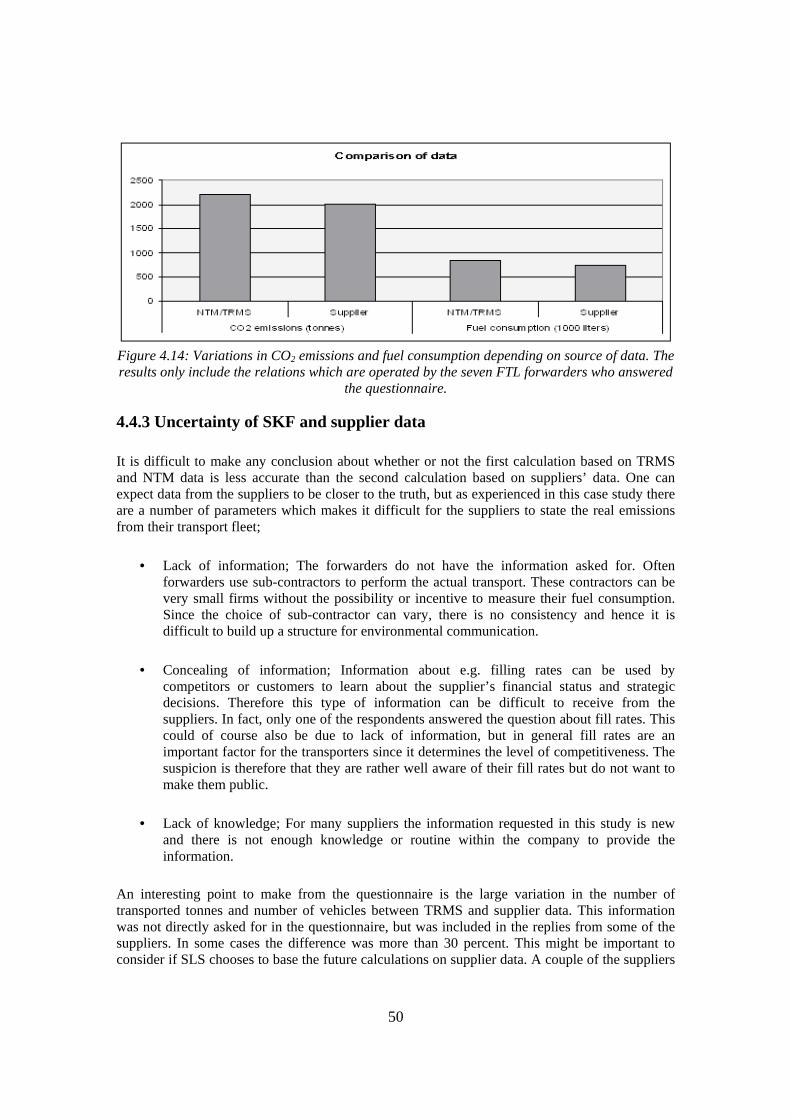
50

Figure 4.14: Variations in CO2 emissions and fuel consumption depending on source of data. The results only include the relations which are operated by the seven FTL forwarders who answered

the questionnaire.

4.4.3 Uncertainty of SKF and supplier data It is difficult to make any conclusion about whether or not the first calculation based on TRMS and NTM data is less accurate than the second calculation based on suppliers’ data. One can expect data from the suppliers to be closer to the truth, but as experienced in this case study there are a number of parameters which makes it difficult for the suppliers to state the real emissions from their transport fleet;

• Lack of information; The forwarders do not have the information asked for. Often forwarders use sub-contractors to perform the actual transport. These contractors can be very small firms without the possibility or incentive to measure their fuel consumption. Since the choice of sub-contractor can vary, there is no consistency and hence it is difficult to build up a structure for environmental communication.

• Concealing of information; Information about e.g. filling rates can be used by competitors or customers to learn about the supplier’s financial status and strategic decisions. Therefore this type of information can be difficult to receive from the suppliers. In fact, only one of the respondents answered the question about fill rates. This could of course also be due to lack of information, but in general fill rates are an important factor for the transporters since it determines the level of competitiveness. The suspicion is therefore that they are rather well aware of their fill rates but do not want to make them public.

• Lack of knowledge; For many suppliers the information requested in this study is new and there is not enough knowledge or routine within the company to provide the information.

An interesting point to make from the questionnaire is the large variation in the number of transported tonnes and number of vehicles between TRMS and supplier data. This information was not directly asked for in the questionnaire, but was included in the replies from some of the suppliers. In some cases the difference was more than 30 percent. This might be important to consider if SLS chooses to base the future calculations on supplier data. A couple of the suppliers

51

also provided calculated CO2 emissions for the SKF goods. Since the input transport activity data was different from the ones used in this study, the CO2 figures were not comparative. The transport data from SKF could be collected in two ways – through the “trip specification list” from TRMS or by using “the Cube”. TRMS is the transport data system and the Cube is an internal tool for statistics within SLS. The Cube consists of modified TRMS data. The basic problem was that TRMS was not built for the purpose of providing raw data for environmental calculations. Manual handling of the data needed to be made, e.g. removing the trucks that are only in the system to make the financial information correct. Hence the Cube data was thought to be more accurate for the purpose of this study since this data has already been modified by people within the company. However, problems were encountered while using the Cube data. The data for the weeks covered in this study was updated retrospectively during the time of data collecting. The data found at the start of the process was therefore not the same as in the end. This made things more complicated and doubts were raised of the reliability of the Cube data. It was apparent that the Cube data was much too high. One example to illustrate the problem is the relation Gothenburg – Tongeren (GOTG). According to information from both SLS and the forwarder, there are 3-6 trailers leaving each week day from Gothenburg to Belgium. However, according to the Cube the number of trailers between week 1 and 26 were 1035, which corresponds to 8 trailers each day. It was assumed that the strange values were the result of some sort of administrative problem. Instead of using Cube data, the trip specification list was manually handled by the authors of this report. The outcome was more in line with forwarder’s data and also much in accordance with other information received at SKF. In the example GOTG above, the manually handled file showed 517 trucks, which are approximately 4 each day. This number seemed to be more true to reality. The advantages and disadvantages with each of the methods of data collection are discussed in table 4.2. These are issues that were raised by the authors during the data collection process for this study.

Table 4.2: Comparison between data collection approaches.

Data collection

Forwarder data

SKF data

Advantages

- The forwarder is generally more aware of the situation specific conditions. - Easy for SKF once all transporters can provide and process data in a standardized way.

- Complete control of both collection and processing of data. - Validation possible. - Could be time saving.

Disadvantages

- Difficult to make all forwarders report in the same way. - Difficult to verify data. - Lack of information/knowledge/ ambition which results in less accurate results.

- Lack of insight in the actual transport chain. - Systems not adjusted for providing transport data for environmental calculations.

52

When discussing the process of data collection it is also important to include the issue of responsibility for the resulting information. Since the information about transport emissions will be spread in a number of ways, e.g. through the annual sustainability report, SKF should be interested in only publishing information they can assume responsibility for in case the data is in some way questioned by an external actor. The more data collection and calculations that are done within the company, the more responsibility SKF assumes in terms of providing correct information. If the calculations are placed on the suppliers, SKF loses control over the information but might not have to defend the data if the data is questioned. SKF can simply say that it is the forwarders' responsibility to provide SKF with reliable information. So, should companies like SKF bother trying to find information from the transport companies? Well, it might not be necessary since the default values seem to work rather well compared to “situation specific information”. From the experience from the questionnaire in this study, the contacts with the suppliers are rather time consuming. The question is if it is worth the extra time spent to get a result which is close to the general calculations which can be done without the transporter information. The more efficient choice in this case is for sure to use the company data only. However, starting up a dialogue with the transport suppliers can be beneficial from other aspects. If the transport suppliers are more pushed to state their environmental performance they might see the possibility to use environmental performance as a competitive advantage and this will urge them to improve in the environmental field. When the relation has been established and the suppliers are able to report according to SKF set standards, the supplier dialogue might not be as time consuming and might also provide more reliable data. Environmental communication with the transport suppliers can also be used in the tendering process. There are examples of companies that rank the suppliers not only based on economic preferences but also on how well they perform in the environmental area. One tool that can be used in this process is QIII, which helps transport buyers to assess transport suppliers’ work within environmental, safety and quality issues (QIII 2007). The transport contract can then receive the QIII quality certificate if it corresponds to the demands. It is still difficult to purchase a more expensive transport just because of environmental reasons, but slowly this might be changing. One example is Tetra Pak who is willing, on a trial basis, to increase the transport costs by two percent. This gives space to choose more environmentally friendly transport alternatives (Rosén 2007).

53

5 Case studies – Improving a logistics system

5.1 Case GOTG – intermodal transport The transports from Gothenburg to Tongeren (GOTG) are interesting from different aspects. The relation has the highest total CO2 impact due to the large volumes of goods. A change in the transport mode could therefore have a relatively large impact on the total emissions from the DTS network. Another interesting aspect is the high fill rates on this relation. Fill rates are often close to 100 percent, which makes GOTG the relation with the lowest emissions in terms of grams CO2 per tonne-km. It is therefore reasonable to question what further emissions improvements that can be made. There are two options; either the mode of transportation is changed or the transport work is reduced. The former is studied here, while the latter is studied in the UK case with different circumstances (see chapter 5.2). In this case study three alternative transport routes are compared with a reference scenario that describes the current set up. The aim is to reduce the road share of the total transport chain without completely disregarding the current transport lead-time of 28 hours. The transported cargo corresponds to a semi-trailer (25 tonnes load capacity) with a fill rate of 99 percent. The underlying data is provided by various sources.13 The following transport chains are studied: Ferry/road: GO hub – Gothenburg port: Tractor and semi-trailer

Gothenburg port – Kiel: Ferry Kiel – Tongeren: Tractor and semi-trailer Estimated total transport lead-time: 24 hours

RoRo/road: GO hub – Gothenburg port: Tractor and semi-trailer

Gothenburg port – Gent (Belgium): RoRo vessel (semi-trailer only) Gent – Tongeren: Tractor and semi-trailer Estimated total transport lead-time: 34 hours

Rail/road: GO hub – Malmö Kombi terminal: Tractor and semi-trailer Malmö Kombi terminal – Duisburg (Germany): Electrical rail (semi-trailer only) Duisburg - Tongeren: Tractor and semi-trailer Estimated total transport lead-time: 30 hours

13 Distances are collected from: ViaMichelin and World Port Distances. The rail service is offered by the logistic company Kombiverkehr. Rail calculations are done with the online tool EcoTransIT. Data concerning the RoRo vessel was provided by DFDS Torline. The ferry is assumed to be Stena Germanica and the necessary technical data is provided by Stena Line.

54

Ref.: GO hub – Rödby (Denmark): Tractor and semi-trailer (Öresund Bridge) Rödby – Puttgarden (Germany): Ferry

Puttgarten – Tongeren: Tractor and semi-trailer The result of the calculation is presented in figure 5.1. The rail/road combination proved to have the lowest CO2 impact, while the RoRo/road and the ferry/road are comparable to the reference scenario.

Figure 5.1: The CO2 impact from each alternative transport chain.

It is important to point out that that different transport chains cover different distances. This is of course due to physical constrains in terms of infrastructure. The actual total performance, measured in g CO2 per tonne-km, of each transport chain and its individual modes are presented in table 5.1. The rail mode is calculated by using the EcoTransIT emission load calculator, in which the emissions are based on national electricity production data. For more details about the assumptions behind the calculations, see section 4.2.3.

Table 5.1: Performance in g CO2 per tonne-km for each transport chain and mode.

Transport chain

Performance [g CO2 per tonne-km] Road Rail RoRo Ferry Total

Ferry/road 37 45 41 RoRo/road 37 43 42 Rail/road 37 19,5 25 Ref. 37 45 38

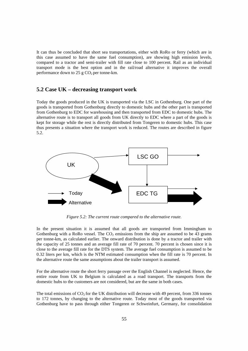
55

It can thus be concluded that short sea transportations, either with RoRo or ferry (which are in this case assumed to have the same fuel consumption), are showing high emission levels, compared to a tractor and semi-trailer with fill rate close to 100 percent. Rail as an individual transport mode is the best option and in the rail/road alternative it improves the overall performance down to 25 g CO2 per tonne-km.

5.2 Case UK – decreasing transport work Today the goods produced in the UK is transported via the LSC in Gothenburg. One part of the goods is transported from Gothenburg directly to domestic hubs and the other part is transported from Gothenburg to EDC for warehousing and then transported from EDC to domestic hubs. The alternative route is to transport all goods from UK directly to EDC where a part of the goods is kept for storage while the rest is directly distributed from Tongeren to domestic hubs. This case thus presents a situation where the transport work is reduced. The routes are described in figure 5.2.

Figure 5.2: The current route compared to the alternative route. In the present situation it is assumed that all goods are transported from Immingham to Gothenburg with a RoRo vessel. The CO2 emissions from the ship are assumed to be 43 grams per tonne-km, as calculated earlier. The onward distribution is done by a tractor and trailer with the capacity of 25 tonnes and an average fill rate of 70 percent. 70 percent is chosen since it is close to the average fill rate for the DTS system. The average fuel consumption is assumed to be 0.32 liters per km, which is the NTM estimated consumption when the fill rate is 70 percent. In the alternative route the same assumptions about the trailer transport is assumed. For the alternative route the short ferry passage over the English Channel is neglected. Hence, the entire route from UK to Belgium is calculated as a road transport. The transports from the domestic hubs to the customers are not considered, but are the same in both cases. The total emissions of CO2 for the UK distribution will decrease with 49 percent, from 336 tonnes to 172 tonnes, by changing to the alternative route. Today most of the goods transported via Gothenburg have to pass through either Tongeren or Schweinfurt, Germany, for consolidation

UK LSC GO

EDC TG Today

Alternative

56

before the last transports to domestic hubs are made. Only about eleven percent of the total goods, in weight, are not transported via Belgium or Germany. The alternative route directly from UK to Tongeren hence cuts off many unnecessary transports between Gothenburg and the continent. The variables in this case study are mainly the assumptions about fuel consumption and fill rate for the transport modes. If the fill rate for the road transport is decreased to 60 percent, the fuel consumption would assumingly be 0.307 liter per kilometer. This would give 364 tonnes with today’s situation and 193 tonnes if the alternative option is chosen, i.e. a 47 percent decrease. If the fill rate is increased to 80 percent, the fuel consumption would be 0.330 liter per kilometer. This would give 317 tonnes of CO2 with today’s situation and 158 tonnes if the alternative option is chosen, i.e. a 50 percent decrease. The emissions from the sea transport can vary substantially, depending on the assumptions made on the vessel, allocation etc. To compare the factor calculated in this study with another factor, the factor for inland transport in the GHG Protocol calculation tool for mobile combustion will be used, 0,035 kg/tonne-km. With the lower value the difference will be 46 percent between the two cases. The sensitivity analysis can be seen in figure 5.3.

Figure 5.3: Sensitivity analysis comparing different fill rates

and emission factors for sea transports.

57

6 Discussion Logistics The transport sector is dominated by discussions about low costs and short lead times to which environmental issues are not always compatible. Some efforts, like improving fill rates, are beneficial both from a financial and an environmental perspective. However, other attempts to reduce environmental impact, e.g. changing from road to rail, will often increase both time and cost. As McKinnon (1994) states; “(both corporations and academic research have) ...established a very solid paradigm of how logistics should be managed to maximize economic returns. The introduction of a new set of environmental objectives threatens to disturb this paradigm”. Several years have passed since McKinnon stated these words, but the conflict between financial and environmental savings is still a pressing issue. Things are starting to happen; there are e.g. forwarders who offer a more environmentally friendly transport solution for a slightly higher cost, but it is still difficult for companies to allow for increased transport costs. The DTS strategy is in line with the principles of JIT and lean production that the industries adopted from the eighties and onward. The principles emphasize the demand for precise transports, delivering at “the right time”, as the carrier is an integral part of the production line (Fricker & Whitford 2004). In practice this has resulted in a demand for fast and flexible transport modes. This corresponds to the cornerstones of the DTS that implies a system completely relying on road transport which is the only mean of transport which is both cost-efficient and fast enough. SKF has locked themselves into a system with strict timetables and short lead times. This makes SKF’s possibility to change modes difficult, if not impossible. Any changes which will imply longer lead time or decreased frequency would worsen the service to the customers. There are no easy solutions to these questions; it’s a matter of making tradeoffs. The problems need to be discussed in collaboration with customers and suppliers. One possible measure in order to increase the utilization of resources is to change the customers’ demand so that the need for transport services is steadier. This can be made by e.g. price differentiation (Lumsden 1995). Price differentiation does exist within SLS already. There are four different types of orders with different priority codes for delivery. The lower the priority the lower the warehousing cost. However, there can be reasons to further differentiate the prices so that customers are forced to make a more active decision. Other possible discussions can be made in the areas of service level and planning. It is common that customers’ pay for a service level they do not require, but they get used to it once the service exists (Blinge 2007). Better planning could be helpful both in order to avoid express deliveries and to increase the overall fill rates of the entire logistics system.

58

Reporting SKF’s reasons to account for carbon dioxide emissions can be tracked to a number of areas; image, ethics, customer demands etc. The reporting is thus going to be used for both internal and external use. As for now, the reporting is completely voluntary, and therefore the methodology is not a crucial issue as long as it is consistent. However, the tables might be turned and in the future the reporting of transport emissions can have other applications than pure stakeholder information. If regulations on transport emissions are introduced, companies who are well prepared might be better off since a structure for monitoring and a plan for improvement already exist. In such a situation it might be rational to not overestimate the company impact until more strict guidelines exist on which emissions to include. Also other scenarios can make it important to make the accounting of emissions better defined. Beyond zero is a concept used by SKF in which the energy reductions customers make by using SKF’s improved technique should cover the SKF emissions. Choices of company boundary and limitations will be important in order to achieve the goal of zero emissions, if the concept should be used practically. It is also interesting to discuss if the concept per se is motivated. Is it reasonable for SKF to take credit for savings at the customers’ facilities? It might be difficult to set boundaries on which emission reductions that should be allocated to SKF. Another aspect, for which methodology is important, is if SKF take on responsibility for compensating for emissions by investing in emission permits or other carbon offsets. Every tonne of CO2 emission that SKF accounts for will then be related to a cost.

Environmental Management SLS today lacks a general overview of the environmental impact caused by the company’s activities. This is essential for further work within this area. A striking example of this is the comparison between emissions from DTS and the global air freight program done in this study. DTS is of course important for SLS, but maybe the plans for energy reducing activities should not only concentrate on increasing fill rates on trailers but also try to decrease the number of air freight shipments. The discussion about the difficulties to include environmental management systems in strategic work can be directly applied to SLS. Hopefully the accounting of transport emissions will be handled in a more structured and dedicated way when the Sustainability Manager position is appointed. To include environmental aspects in the purchasing of transports could be an interesting approach for future work. By starting up a dialogue with the transporters, more demands can be set and hence the environmental impact can be reduced in a long-term perspective. It could also be interesting to rank different transporters depending on their environmental performance and to let this be an aspect to consider in the purchasing decision.

59

Data The data collection was one of the major challenges for the accounting process in this study. The scientific methods and default values have built in problems per se, e.g. the categorization of trucks, inclusion or exclusion of lifecycle data and the generalizations of fuel consumption. For these variations a clear boundary can be set, i.e. the company simply chooses a method or approach and then works according to it. It is important that decision makers are aware of the underlying premises of the calculations so that no sub optimization is done. However, a larger problem than setting boundaries to scientific methods was to collect data on transport activity. Since the data has not been used for environmental calculations before, the systems are not adapted for it. There seems to be a lack of reliable information about the real amount of transported goods or vehicles used, since the trip specification list also has to include corrections connected to economic aspects. This situation is not unique to SKF. According to Pålsson (2006), environmental information is generally not central business information within organizations. “The relationship between business development and environmental information is generally not well understood and established. This often hampers availability and accessibility of the information that is needed”. A recommendation to SLS would be, as a first step, to look over the transport activity data to see if it can be made more reliable and consistent. The Cube proved to be a very efficient way of collecting data, but unfortunately it was not possible to use it due to the apparent reliability problems as discussed in section 4.4.3. However, an improved and extended database would be very helpful for future transport calculations. To gather all transport activity data in one place assures that everyone in the company uses the same data and that changes in the data can be tracked over time. Preferably the existing SKF database, SKF Compass, could be extended to also include freight transports. A second recommendation is to start a more active exchange of environmental information with the forwarders. It would be helpful with a standardized format for which environmental performance should be presented by the supplier. As seen from the questionnaires, it might take a while before all transporters can provide reliable transport information, but a standardized format is a first step.

Coordination of activities The SKF Group Sustainability is a good initiative and seems to have made a large contribution to the SKF Group’s performance within the area of sustainability. However, for accounting of transport emissions, there seems to be a lack of coordination both at top management and at SLS. There is a great interest in the issue, from many different directions, and the impression is that many local initiatives have already been taken. However, there is no general method or manual to use. A recommendation is therefore to construct a group wide manual on how to perform calculations and how to handle e.g. system boundaries. This would result in a more consistent accounting. Hopefully the sustainability manager at SLS could contribute to this. However, also in the sustainability group there should probably be someone with “transport knowledge” since

60

transports are carried out throughout the whole SKF Group, and not only under SLS´ responsibility.

Weaknesses in methodology A general problem for the calculations in this study is that there is no exact guideline to follow. As Bäckström (2007) states; “there is no general scientific method that always can be used”. Since it is not possible to measure the exact emissions for each transport, with the current situation, all results will be based on a number of assumptions. What is right or wrong is difficult to judge. In some cases, e.g. allocation, several methods can be chosen even though some methods are more acknowledged than other. The results are therefore always, to a certain extent, subjective and influenced by the individual’s approach to the problem. NTM has been used to a great extent during the course of this study, and it might be a limitation to the study. However, an extensive discussion about the uncertainty of the input data has been carried out, and other studies have been looked at through the course of the study. The uncertainty of the emission calculation result for DTS was illuminated by the sensitivity analysis in chapter 4.4.1. Uncertainties cannot be completely avoided but with a sophisticated method for estimating possible variations the resulting deviations will be more reliable. For the parameters which are clearly related with uncertainties a random selection of trips can be examined and precisely measured. Although the NTM default value for fuel consumption does account for some situation specific variations, this is the parameter assumed to be associated with most uncertainty. This should be considered when performing a sensitivity analysis, which is always recommended (NTM 2007). The questionnaire to forwarding companies was an attempt to gather data to get a better, more situation specific, calculation. However, the responses were in many cases not informative and overall only half of the forwarders replied. A problem could be that the participants answering the questionnaire might have misinterpreted the questions or simply did not answer due to lack of time or knowledge. However, the authors tried to present the questions in a straight forward way and gave the companies possibilities to ask questions. Due to a somewhat changed direction of this study, some of the questions in the questionnaire were not directly relevant for the results in this study. However, these answers could still provide a general picture of the situation for the suppliers today. The discussions in this study have been limited to carbon dioxide emissions since this is the main focus for SKF today. Other transport emissions are also important to consider.

61

7 Final conclusions Corporate environmental management accounting is often connected to monitoring and improving core business areas of the company, usually according to an environmental management standard. The driving forces for SKF are connected to stakeholder pressure and business opportunities, which is in line with research (e.g. Kolk 2000). The growing interest for transport emissions at SKF is partly due to a general interest in mapping the company related emissions with the belief; “what you can measure, you can manage” (Jenkinson 2007). It is thought to help SKF prioritize and focus the energy reducing efforts. To stay competitive is another driving force. The environmental impact from freight transports could be handled within the frame of the Environmental Management System (EMS) on site level, if e.g. the Logistics Service Center (LSC) in Gothenburg starts to work actively on the EMS goal to include transport emissions. However, it is important that also the strategic departments play a larger role in the environmental management work since this is where the underlying premises of the transport system can be changed. Another recommendation is to use environmental claims already in the tender process and at all times have an ongoing debate with the forwarders concerning alternative routes and transport modes that might lead to decreased environmental impact. At SKF Logistics Services (SLS) there is currently a position being created in order to enhance sustainability management. This gives an opportunity to create a common working method within the company and support the sites, e.g. the LSC in Gothenburg, to fulfill their EMS commitment to transport emissions. Carbon dioxide emissions from transports can be calculated in a number of different ways, and which way is appropriate depends on the resources dedicated to the issue within the company. A final conclusion from this study is that there is much space for companies to set their own boundaries and make assumptions convenient for the company. However, with an intensified debate on global warming the rules might change and a more concrete standard on how to account for emissions might be established. It could therefore be recommended for companies to closely follow the ongoing discussion in this field. As a first step, it could be beneficial for SKF to continue the mapping of their entire transport system in order to find the weak spots. Important to remember is that the Daily Transport System (DTS) is a small part of the total transport system and also a relatively efficient system. Changing parts of one system without having the knowledge of the total system, might lead to sub-optimization. However, when the transport system is better mapped, changes in the system should be considered and implemented. The cases in this study show that improvements can be done both by changing transport modes and by optimizing the logistics system by decreasing transport work. The barriers to this development originate from the logistics system’s characteristics. Issues like lead-time, warehousing capacity and costs are interconnected and thus introducing changes will affect the entire system. Other barriers to change can be political decisions within the company or the lack of knowledge, time and available transport alternatives.

62

8 References 8.1 Published Ammenberg, J. (2004). Miljömanagement. Studentlitteratur, Lund Arrhenius, S. (1896). On the influence of carbonic acid in the air upon the temperature of the ground. Philosophical Magazine and Journal of Science Series 5, Volume 41, p. 237-276. Axelsson, M., and Dahlqvist, J. (1999). SKF European Distribution Structure – Analysis and improvement potential. Report 1999:63, Department of Management and Economics. Linköping: Linköping Institute of Technology. Baumann , H., and Tillman, A-M. (2004). The hitch hiker’s guide to LCA. Studentlitteratur, Lund. Blinge, M., Arnäs, P.O., Bäckström, S., Furnander, Å., Hovelieus, K. (1998). Life-cycle assessment of motor fuels – Present best available technology and a future scenario for Sweden. 8th World conference of transportation research, Antwerp, Belgium, 12-16 July 1998. Carlsson, N., Olofsson, A., Andersson, S. (2003) Emissionsberäkning för Flöde Göteborg – Airasca. SKF Logistics Services Göteborg. CDP (2006). Carbon Disclosure Project Report 2006: Global FT500. Report is accessible from CDP web page. http://www.cdproject.net/reports.asp (2007-10-24). EIA (2007). International Energy Outlook 2007. Energy Information Administration, US Department of Energy, Washington DC, 2007. Ekdahl, Å. (2001). Life cycle assessment on SKF’s spherical roller bearing. Report 2001:1, Department of Environmental Systems Analysis, Göteborg: Chalmers University of Technology. Elkington, J., Hailes, J. (1991). The green business guide. Victor Gollancz, London. Erlandsson, J. (2006). Company and product related environmental information management. Report: 2006:3.Department of Environmental Systems Analysis, Göteborg: Chalmers University of Technology. Fricker, J., Whitford, R. (2004). Fundamentals of Transportation Engineering. Pearson Education Limited, New Jersey. Friedrich, R., Bickel, P. (2001). Environmental external costs of transports. Springer-Verlag, Berlin. Frischknecht, R., Althaus, H-G., Bauer, C., Doka, G., Heck, T.,Jungbluth, N., Kellenberger, D., Nemecek, T. (2007). The environmental relevance of capital goods in life cycle assessment of products and services. Int J LCA 2007 (OnlineFirst):11. IFEU (2005). EcoTransIT: Environmental methodology and data. Institute fur Energie und Umweltforschung, Heidelberg

63

IEA (2006). World Energy Outlook 2006. International Energy Agency publications, Paris. IVA (2002). Energianvändning i transportsektorn. IVA rapport, Multitryck, Eskilstuna. IVL (2001). Miljöfaktabok för bränslen –del 2. Bakgrundsinformation och teknisk bilaga. IVL rapport: B 1334b-2, Stockholm. IVL (2002). Strukturerad miljödatahantering inom järn- och stålindustri. IVL report: B1471. IVL Svenska miljöinstitutet AB, Stockholm. Jackson, A., Jackson, J. (2000). Environmental Science. 2nd ed. Pearson Education Limited, Harlow. Johansson, S., Mellqvist, J. (2007). Towards sustainable business travels. Report: 2007:13. Department of Environmental Systems Analysis, Göteborg: Chalmers University of Technology. Järnvägsforum (2004). En konkurrenskraftig svensk järnväg. www.jarnvagsforum.se/pdf/Konkurrenskraft.pdf Kolk, A. (2000). Economics of environmental management. Pearson Education Limited, Harlow. Lash, J., Wellington, F. (2007). Competitive advantage on a warming planet. Harvard Business Review, Mars 2007, p. 95-102. Lumsden, K. (1998). Logistikens grunder. Studentlitteratur, Lund. Lumsden, K. (1995). Transportekonomi. Studentlitteratur, Lund. McKinnon, A.C. (1994). Logistics and the environment. EUROLOG, Brussels, 13 November 1994). NTM (2007). Environmental data for international cargo transport- road. Version 2007-04-13, www.ntm.a.se (2007-07-10). NTM (2007). Environmental data for international cargo transport – air. Version 2007-08-10, www.ntm.a.se (2007-10-22). OECD (2006). Decoupling the environmental impacts of transport from economic growth. Retrieved from the OECD Environmental transport database (2007-08-10). Pålsson, A. (2006). Information quality in industrial environmental management. Report: 2540. Department of Computer Science and Engineering, Göteborg: Chalmers University of Technology. Porter, M., Kramer, M. (2006). Strategy and Society: The link between competitive advantage and corporate social responsibility. Harvard Business Review, December 2006, p. 78-92. SIKA (2007). Kilometre tax for lorries: Effects on industry and regions. SIKA report 2007:2, Stockholm, 2007. SKF (2007) Annual Report 2006 including sustainability report. AB SKF and Admarco.

64

Svending, O. (2003). Industrial management of environmental data. Report: 2003:14. Department of Environmental Systems Analysis, Göteborg: Chalmers University of Technology. TFK (1998). Environmental impact of transports: environmental handbook of purchasing. Institut för transportforskning, Stockholm. Swedish EPA (2003). Effektivare miljöledningssystem. Report: 5304. Naturvårdsverket, Stockholm. Welford, R., (1998). Corporate Environmental Management. Revised ed. Earthscan Publications Limited, London. 8.2 Websites ASPO (2007). The Association for the study of peak oil and gas: Newsletter No. 82. The Association for the Study of Peak Oil and gas. http://www.peakoil.net (2007-10-20). DHL (2007). Välkommen till DHL Sverige. DHL Sweden. www.dhl.se (2007-10-22). EC (2007). Aviation and climate change. The European Commission. http://ec.europa.eu/environment/climat/aviation_en.htm (2007-10-22). EcoTransIT (2007). EcoTransIt Environmental Load Calculation. Green Cargo. http://www.ecotransit.org (2007-08-20). EEA (2007). EEA multilingual environmental glossary. European Environment Agency. http://www.eea.europa.eu (2007-10-20). Transport and Environment (2007). Emissions trading for shipping: “not enough” to tackle climate change. European Federation for Transport and Environment. http://www.transportenvironment.org (2007-10-20). Greenhouse Gas Protocol (2003) Mobile Combustion CO2 Emission Calculation Tool. Version 1.2 WRI-WBC-SD, Greenhouse Gas Protocol Initiative, Calculation tools, www.ghgprotocol.org (2007-09-20). Global Reporting Initiative (2007). About GRI. Global Reporting Initiative. http://www.globalreporting.org (2007-10-20). IPCC (2007). Fourth assessment report (WG III AR4). International Panel of Climate Change. The report is accessible at: http://www.mnp.nl/ipcc/pages_media/ar4.html (2007-10-20). Kombiverkehr (2007). Willkommen bei Kombiverkehr. Kombiverkehr. www.kombiverkehr.de (2007-10-20). Kuehne and Nagel (2007). Airfreight. Kuehne and Nagel Group. http://www.kn-portal.com/en/forwarding/airfreight (2007-10-22). The Nobel Foundation (2007) The Nobel Peace Prize 2007. The Nobel Foundation.

65

http://www.nobelprize.org (2007-10-23). Schenker (2007). Logistikmagasinet juni 2007. Schenker AB. www.schenker.se (2007-10-22). SKF intranet (2007). SKF Group. www.skf.se (2007-10-20) Spannagle, M. (2004). A Comparison of ISO 14064 Part 1 and the GHG Protocol Corporate Module. http://www.ecologia.org/ (2007-08-10). Statoil (2007). Frågor och svar kring diesel. Statoil Sverige AB. http://www.statoil.no/MAR/svg01184.nsf/docs/info_europadiesel_faq (2007-10-01). Stena Line (2007). Stena Germanica. Stena Line Sverige. http://www.stenaline.se (2007-10-20) Swedish Environmental Protection Agency (2007). Klimat i förändring. Naturvårdsverket. http://www.naturvardsverket.se (2007-10-10) Swedish Road Administration (2007). Vägverket. www.vagverket.se (2007-09-02). Via Michelin (2007). Driving directions. Michelin Group. www.viamichelin.com (2007-09-05). Volvo (2007). Volvo emission factors. Volvo Group. www.volvo.com (2007-10-23). World airport codes (2007). Welcome to world airport codes. www.world-airport-codes.com (2007-10-22). World Port Distances (2007). World Ports Distances Calculator. www.distances.com (2007-10-20). QIII (2007). Kvalitet i upphandling av vägtransporter. Quality Three Organization. www.q3.se (2007-10-12). 8.3 Personal communication Andersson, Ulf (2007). SKF, Environmental Coordinator SKF Sweden. Axelsson, Mattias (2007). SKF, Manager Quality, Packaging & Adm. Service, SKF Logistics Serveices Gothenburg. Belin, Sören (2007). Green Cargo, CEO. Oral presentation at the seminar “Sustainable Transports” Stockholm 2007-10-11, organized by IVL Swedish Environmental Research Institute in cooperation with the Network for Transport and Environment. Blinge, Magnus (2007). Nätverket för transporter och miljö (NTM), member of the NTM board. Bäckström, Sebastian (2007). Nätverket för transporter och miljö (NTM), author of NTM reports. Jenkinson, Rob (2007). SKF, Project Manager, Group Sustainability.

66

Karlsson, Lennart B. (2007). SKF, Transport Coordination Manager – East Europe and Middle East, SKF Logistics Services. Löfgren, Birger (2007). Project Engineer PhD. Candidate, Group Technology Development & Quality/MDC/Environment SKF Nilsson, Marie (2007). DFDS Torline. Ohlsson, Yngve (2007). SKF, Vice president, Transports, SKF Logistics Services. Olsson, Stefan (2007). SKF, Manager, Customer Service & Supply Chain, Customer Service. Rosén, Ulrika (2007). Tetra Laval, Group Transport and Travel. Oral presentation at the seminar “Sustainable Transports” Stockholm 2007-10-11, organized by IVL, Swedish Environmental Research Institute, in cooperation with the Network for Transport and Environment. Swahn, Magnus (2007). Nätverket för transporter och miljö (NTM), head of the NTM board. Toepfer, Juergen (2007). SKF, Global Product Manager Road Freight, SKF Logistics Services.

I

Appendix 1 Definitions: Environmental Management Accounting: The process of identifying, measuring, accumulating, analyzing, preparing, interpreting, and communicating environmental information. (Svending 2003) Forwarding agent: a supplier providing entire logistics solutions, often in cooperation with sub-contractors. Hauler: a sub-contracted supplier of transport services Traffic work: vehicles multiplied with distance (e.g. vehicle-km) Transport work: transported weight multiplied with distance (e.g. tonne-km) Inbound transports: Transportation of goods from material suppliers to production sites Outbound transports: Transportation of finished products to final customers Abbreviations: DTS: Daily Transport System EDC: European Distribution Center FTL: Full Truck Load GHG: Greenhouse gases LSC: Logistics Service Center LTL: Less than Truck Load OEM: Original Equipment Manufacturer SLS: SKF Logistics Services

II

Appendix 2 Comment: SKF Logistics Services is here abbreviated SKF LS. Questionnaire FTL The questions concern the specific transports dedicated to SKF Logistics Services (SKF LS), thus the Full Truck Load transport service that your company provide for SKF LS. Please answer as detailed as possible. If you of any reason lack such specific data, we are also interested in more general figures. If your company has more than one transport route dedicated to SKF LS, please list the routes separately in your answers. 1. Do you know the exact fuel consumption (l/km) for the transport dedicated to SKF LS? If yes, what is the fuel consumption and how is this number derived? If no, do you have an average number for fuel consumption? How is it derived? 2. Do you know the exact consumption (liters of fuel per vehicle) for the transport routes dedicated to SKF LS? If yes, how large is the consumption per trip? 3. What exact distance does the transport dedicated to SKF LS cover? 4. Which types of vehicles (maximum weight) are used for the transport route dedicated to SKF LS? 5. Which type of fuel is used for the transport route dedicated to SKF LS (degree of sulphur content)? 6. Which EURO class do the vehicles used for the transport dedicated to SKF LS have? 7. What is the estimated fill rate for the return loads (if the return loads are not SKF dedicated goods)? 8. Have your company carried out any measures to decrease your environmental impact? Please, send your answers by e-mail to: christian.stenqvist@skf.com For doubts or any kind of questions you are most welcome to contact us: Christian Stenqvist and Helen Lindblom, Masters Thesis Students, SKF LS Tel: +46 (0)31 33 71 021 E-mail: Christian.stenqvist@skf.com The questionnaire has been approved and supported by: Jürgen Töpfer, Global Product Manager Road Freight, SKF LS

III

Appendix 3 Comment: SKF Logistics Services is here abbreviated SKF LS. Questionnaire LTL The questions concern the Less than Truck Load transportations that your company carry out for SKF Logistics Services (SKF LS). Please answer as detailed as possible. If you of any reason lack such specific data, we are also interested in more general figures. If your company has more than one transport route with SKF LS goods, please list the routes separately in your answers. 1. Do you know the exact fuel consumption (l/km) for the transport route that you carry out with SKF LS goods? If yes, what is the fuel consumption and how is this figure derived? If no, do you have an average number for fuel consumption? How is it derived? 2. Do you know the exact consumption (liters of fuel per vehicle) for the transport routes carrying SKF LS goods? If yes, how large is the consumption per trip? 3. What exact distance does the transport route carrying SKF LS goods cover? If the route includes one or several ferry transports state the following: i) Port of departure and port of destination. ii) The name of the shipping company carrying you cargo carrier. 4. Which types of vehicles (maximum weight) are used for the specific transport route with SKF LS goods? 5. Which type of fuel is used for the transport route (degree of sulphur content)? 6. Which vehicle EURO-class is used on the specific route? 7. What is your estimated fill rate? 8. Have your company carried out any measures to decrease your environmental impact? Please, send your answers by e-mail to: christian.stenqvist@skf.com For doubts or any kind of questions you are most welcome to contact us: Christian Stenqvist and Helen Lindblom, Masters Thesis Students, SKF LS Tel: +46 (0)31 33 71 021 E-mail: Christian.stenqvist@skf.com The questionnaire has been approved and supported by: Jürgen Töpfer, Global Product Manager Road Freight, SKF LS

IV

Appendix 4 SKF Group organization (Source: SKF intranet 2007)

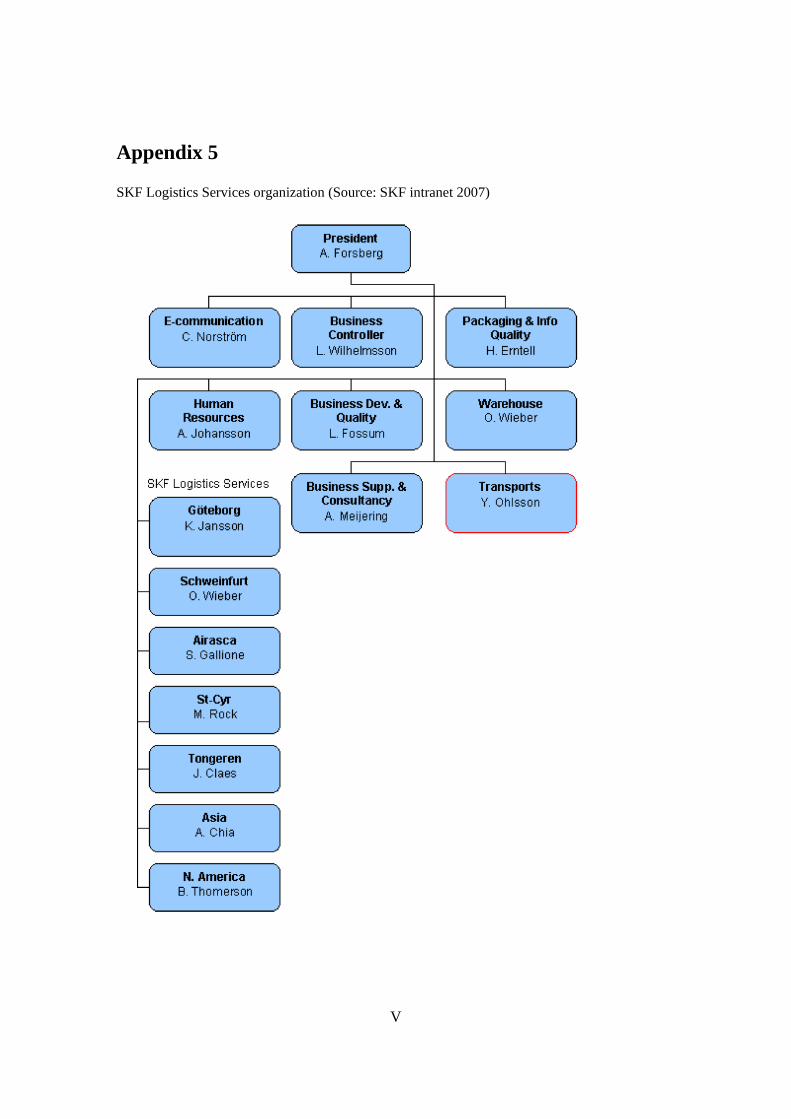
V

Appendix 5 SKF Logistics Services organization (Source: SKF intranet 2007)

VI

Appendix 6 Explanation of the DTS relations – Full Truck Load, FTL:

Departure Arrival Relation Location Country Location Country

AISW Airasca Italy Schweinfurt Germany

AITG Airasca Italy Tongeren Belgium

AITO Airasca Italy Tours France

GOAI Gothenburg Sweden Airasca Italy

GOMA Gothenburg Sweden Madrid Spain

GOPA Gothenburg Sweden Paris France

GOSW Gothenburg Sweden Schweinfurt Germany

GOTG Gothenburg Sweden Tongeren Belgium

LCSW Luechow Germany Schweinfurt Germany

LCTG Luechow Germany Tongeren Belgium

MATO Madrid Spain Tours France

STSW Steyr Austria Schweinfurt Germany

SWAI Schweinfurt Germany Airasca Italy

SWGO Schweinfurt Germany Gothenburg Sweden

SWST Schweinfurt Germany Steyr Austria

SWTG Schweinfurt Germany Tongeren Belgium

SWTO Schweinfurt Germany Tours France

TGAI Tongeren Belgium Airasca Italy

TGED Tongeren Belgium Ede The Netherlands

TGFW Tongeren Belgium Friedewald Germany

TGGO Tongeren Belgium Gothenburg Sweden

TGMU Tongeren Belgium Muelheim Germany

TGNH Tongeren Belgium Northampton UK

TGPA Tongeren Belgium Paris France

TGPX Tongeren Belgium Paris Express France

TGSW Tongeren Belgium Schweinfurt Germany

TGTO Tongeren Belgium Tours France

TOAI Tours France Airasca Italy

TOMA Tours France Madrid Spain

TOSW Tours France Schweinfurt Germany

TOTG Tours France Tongeren Germany

VELC Veenendal The Netherlands Luechow Germany

VESW Veenendal The Netherlands Schweinfurt Germany

VII

Appendix 7 Explanation of the DTS relations – Less than Truck Load, LTL:

Departure Arrival Relation Location Country Location Country

AIAT Airasca Italy Athens Greece

AVTO Avallon France Tours France

GOGO Gothenburg Sweden Gothenburg Sweden

GOHE Gothenburg Sweden Helsinki Finland

GOOS Gothenburg Sweden Oslo Norway

HERI Helsinki Finland Riga Latvia

HETA Helsinki Finland Tallinn Estonia

HEVL Helsinki Finland Vilnius Lithuania

NITG Nieuwegein The Netherlands Tongeren Germany

SWBB Schweinfurt Germany Belgrade Serbia

SWFI Schweinfurt Germany Foscani Romania

SWIS Schweinfurt Germany Istanbul Turkey

SWPZ Schweinfurt Germany Poznan Poland

SWSK Schweinfurt Germany Stip Macedonia

SWSY Schweinfurt Germany Sofia Bulgaria

SWTZ Schweinfurt Germany Tuzla Bosnia

SWWI Schweinfurt Germany Vienna Bulgaria

SWVZ Schweinfurt Germany Varazdin Croatia

TGBA Tongeren Belgium Basel Switzerland

TOTU Tours France Tudela Spain

WIBP Vienna Austria Budapest Hungary

WIBV Vienna Austria Bratislava Slovakia

WILB Vienna Austria Ljubljana Slovenia

Connected to the last years’ focus on climate change, the interest for corporate accounting of greenhouse gas emissions has increased. The main focus for manufacturing companies has been to monitor and reduce the facility related emissions. However, the interest for process related emissions, e.g. from transports, is growing. SKF is one among many companies trying to achieve a greater knowledge in this field. Since the issue of transport emission accounting is rather new, the existing guidelines and methods are not giving full support to companies. This study is contributing with a more hands on guide to emission accounting and the problems associated with it. The areas of transport data handling, emission calculation methodology and emission accounting principles as well as strategic discussions about environmental management are presented. The target groups for this study are mainly SKF employees, but the information could be valuable also for other companies and individuals working with environmental management.