size proportional venn diagrams in 2 and 3 dimensions: … · use venn diagram circles and the...
TRANSCRIPT

Size proportional Venn diagrams in 2
and 3 dimensions:
vennplot(...) in R
by
Zehao Xu
A research paperpresented to the University of Waterloo
in partial fulfillment of therequirement for the degree of
Master of Mathematicsin
Computational Mathematics
Supervisor: Prof. Wayne Oldford & Prof. Marius Hofert
Waterloo, Ontario, Canada, 2017
c� Zehao Xu. Public 2017

I hereby declare that I am the sole author of this report. This is a true copy of the report,including any required final revisions, as accepted by my examiners.
I understand that my report may be made electronically available to the public.
ii

Abstract
Venn diagrams are popular ways to visualize sets. Wilkinson [48] and Frederickson[18] have introduced statistical models for fitting size-proportional Venn diagram. In thispaper, we will improve their methods in several aspects. An R function vennplot() isavailable to provide both 2D and 3D layout.
iii

Acknowledgements
I would like to thank my supervisor, Professor R. Wayne Oldford. Thanks for hispatience and I do learned a lot from him. He gave me a lot of useful suggestion andtechnical help in R. This paper is impossible without his help; thanks Prof Martin Lysy,he gives me a lot of help on C++; I am also appreciate Prop Marius Hofert’s help onmodifying this paper.
iv

Table of Contents
List of Figures vii
1 Introduction 1
1.1 Venn and Euler diagrams . . . . . . . . . . . . . . . . . . . . . . . . . . . . 21.2 Examples of Venn diagrams drawn from the scientific literatures . . . . . . 4
2 Automated construction of Circular Venn diagrams 7
3 Shrink or stretch 20
4 Three dimension Venn diagram 28
5 Unspecified intersections 31
5.0.1 Common case . . . . . . . . . . . . . . . . . . . . . . . . . . . . . . 315.0.2 Special case . . . . . . . . . . . . . . . . . . . . . . . . . . . . . . . 315.0.3 Weight . . . . . . . . . . . . . . . . . . . . . . . . . . . . . . . . . . 36
6 Undirected connected components 38
6.1 Divide G . . . . . . . . . . . . . . . . . . . . . . . . . . . . . . . . . . . . . 416.2 Detect case . . . . . . . . . . . . . . . . . . . . . . . . . . . . . . . . . . . 426.3 Unite G . . . . . . . . . . . . . . . . . . . . . . . . . . . . . . . . . . . . . 43
7 Examples 49
v

8 Comparison with other Venn algorithms 52
9 Discussion 62
10 Appendix 64
vi

List of Figures
1.1 Number of articles containing “Venn diagram” over time from the journalsGenetics and Nature . . . . . . . . . . . . . . . . . . . . . . . . . . . . . . 2
1.2 Venn diagrams with 2,3,4 and 5 sets, respectively [45] . . . . . . . . . . . . 3
1.3 Five possible ways contain all the cases of two circles. Euler diagram isabove and Venn diagram is below. I) a \ b = ?; II) a \ b; III) a = b; IV)a \ b = a; V) a \ b = b. . . . . . . . . . . . . . . . . . . . . . . . . . . . . . 3
1.4 (a) Illustrating the number of unique and shared wMel genes matching thesefour components. [27]. (b) Genes sharing by five asterid species [41]. . . . . 4
1.5 (a) Venn diagram of gene sharing by six woody species [41]. (b) Showingthe number of genes shared between isolates from investigative patients[7]. 5
1.6 (e) Illustrating the overlapping of gene ontology between the highland andsub-highland lineages [49]. (f) Explaining the friendships through locations,ages and interests. (data source: www.livejournal.com) [25]. . . . . . . . . 6
2.1 locate circles with target distance dij . . . . . . . . . . . . . . . . . . . . . 8
2.2 The initial point configuration of data set Figure 1.4 (a), Figure 1.6 (e) and(f) by Jaccard distance . . . . . . . . . . . . . . . . . . . . . . . . . . . . . 9
2.3 The final point configuration of data set Figure 1.4 (a), Figure 1.6 (e) and(f), with stress, 0.00048, 6⇥ 10
�6 and 0.0029 . . . . . . . . . . . . . . . . . 11
2.4 The final layout of disjoint set I(S)?1
by venneuler() of Wilkinson. . . . . 12
2.5 Two dimension circles . . . . . . . . . . . . . . . . . . . . . . . . . . . . . . 13
2.6 The initial point configuration of data set Figure 1.4 (a), Figure 1.6 (e) and(f) . . . . . . . . . . . . . . . . . . . . . . . . . . . . . . . . . . . . . . . . 14
vii

2.7 (a) If Si \ Sj = ?, the way to position Bi and Bj. (b) If Si \ Sj = Si orSi \ Sj = Sj, the way to position Bi and Bj. . . . . . . . . . . . . . . . . 15
2.8 The final point configuration . . . . . . . . . . . . . . . . . . . . . . . . . . 17
2.9 The layout of disjoint set I(S)?1
by venn.js() Frederickson . . . . . . . . 18
2.10 Comparison of success rate and running time [19] . . . . . . . . . . . . . . 19
3.1 Stretch circles with � = 2 or shrink circles with � = 0.5. . . . . . . . . . . . 20
3.2 (a), (e) and (f) corresponds to Figure 1.4 (a), Figure 1.6 (e) and (f) . . . . 25
3.3 The layout of disjoint set I(S)?1
by vennplot() . . . . . . . . . . . . . . . 26
3.4 Scatter plot. Red dots represent venneuler(), blue dots represent vennplot()and purple dots represent vennjs(); imaginary line represents y = 0. Foursets are on behalf of Figure 1.4 (a), Figure 1.6 (e), (f) and I(S)?
1
. . . . . 27
4.1 Dimension p = 3 . . . . . . . . . . . . . . . . . . . . . . . . . . . . . . . . 28
4.2 (a.1) and (a.2) are the same layout but observed by different angles of dataset Figure 1.4 (a); (e) and (f) are the corresponding 3D layout of Figure 1.6(e) and (f) . . . . . . . . . . . . . . . . . . . . . . . . . . . . . . . . . . . . 30
5.1 (a) venneuler() (b) venn.js() . . . . . . . . . . . . . . . . . . . . . . . . 32
5.2 vennplot(twoWayGenerate = TRUE) . . . . . . . . . . . . . . . . . . . . . 35
5.3 vennplot() with high weight on three way intersection . . . . . . . . . . . 36
5.4 scatter plot with high weight on three way intersection, red dots representvenneuler, blue ones represent vennplot(), purple ones represent venn.js 37
6.1 (a) venneuler() (b) venn.js() . . . . . . . . . . . . . . . . . . . . . . . . 39
6.2 vennplot() . . . . . . . . . . . . . . . . . . . . . . . . . . . . . . . . . . . 40
6.3 The choice of cj and x . . . . . . . . . . . . . . . . . . . . . . . . . . . . . 44
6.4 Translation cj . . . . . . . . . . . . . . . . . . . . . . . . . . . . . . . . . . 45
6.5 Translation . . . . . . . . . . . . . . . . . . . . . . . . . . . . . . . . . . . 46
6.6 Rotation . . . . . . . . . . . . . . . . . . . . . . . . . . . . . . . . . . . . . 48
7.1 sharks data frame . . . . . . . . . . . . . . . . . . . . . . . . . . . . . . . . 49
viii

7.2 Multiple groups in one data set . . . . . . . . . . . . . . . . . . . . . . . . 50
7.3 Figure 1.4 (b) data set . . . . . . . . . . . . . . . . . . . . . . . . . . . . . 51
8.1 venneuler()- vennplot(), abs and stress . . . . . . . . . . . . . . . . . . 52
8.2 venneuler() - vennplot(), stress(k), where 1 k m� 1 . . . . . . . . 53
8.3 venneuler()- vennplot(), stress(m) . . . . . . . . . . . . . . . . . . . . . 54
8.4 venneuler()- vennplot(), � . . . . . . . . . . . . . . . . . . . . . . . . . 55
8.5 venn.js() - vennplot(), abs and stress . . . . . . . . . . . . . . . . . . . 55
8.6 For set I(S)?4
. . . . . . . . . . . . . . . . . . . . . . . . . . . . . . . . . . 56
8.7 venneuler()- vennplot(), stress multiple groups . . . . . . . . . . . . . . 57
8.8 (a) is the initial configuration and (b) is the final one . . . . . . . . . . . . 58
8.9 eulerr() - vennplot() . . . . . . . . . . . . . . . . . . . . . . . . . . . . 58
8.10 eulerr() - vennplot(), � . . . . . . . . . . . . . . . . . . . . . . . . . . . 59
8.11 eulerr() - vennplot(), stress(k) where 1 k m� 1 . . . . . . . . . . 60
8.12 eulerr() - vennplot(), stress(m) . . . . . . . . . . . . . . . . . . . . . . 61
9.1 small stress but fit bad . . . . . . . . . . . . . . . . . . . . . . . . . . . . . 63
ix

Chapter 1
Introduction
“Good diagrams clarify. Very good diagrams force the ideas upon the viewer.The best diagrams compellingly embody the ideas themselves.”Wayne Oldford [9]
Venn diagrams are criticized for the use in probability, but they are good for sets [9].In this paper, we consider sets. Chow and Ruskey [11] develop ways to construct area-proportional Venn diagrams. This improvement has great ability to convey the informationfrom sets. In recent years variations of Venn diagrams have increasing be used in scientificpublications, particularly in genetic applications. For example, Figure 1.1
1

Figure 1.1: Number of articles containing “Venn diagram” over time from the journalsGenetics and Nature
shows the results of an online search for “Venn diagram” over all articles appearing inthe journals Nature and Genetics (including G3: Genes, Genomes, Genetics) from 1998to 2017. As can be seen, there has been nearly a 10-fold increase since the turn of thecentury.
1.1 Venn and Euler diagrams
Venn diagrams for m component sets contain all possible 2
m intersections . The are con-structed using multiple closed curves, like circles, ellipses, and other irregular polygonswhich overlap each other to show the various intersections. The interior of a closed curve
2

represents the elements of the set, while the exterior represents the complement of this set[45]. Figure 1.2 shows some Venn diagram examples:
Figure 1.2: Venn diagrams with 2,3,4 and 5 sets, respectively [45]
In contrast to Venn diagrams, Euler [15] only contains the relevant relations whenpresenting sets. In Venn diagrams, a shaded zone may represent non-intersection, but inEuler diagrams, the corresponding zone is usually missing. Figure 1.3 shows the differencebetween Euler diagrams and Venn diagrams for two circles.
I II III IV V
Figure 1.3: Five possible ways contain all the cases of two circles. Euler diagram is aboveand Venn diagram is below. I) a\ b = ?; II) a\ b; III) a = b; IV) a\ b = a; V) a\ b = b.
Initially, Venn and Euler diagrams were designed for symbolic logic (not for sets) withdifferent purposes. Euler diagrams are to demonstrate the known content, but Venn di-agrams are to derive the content [9]. As formal set theory developed, Venn and Euler
3

diagrams became useful tools to embody the relationship between sets. In this paper, inkeep with common use, we will call them Venn diagrams.
1.2 Examples of Venn diagrams drawn from the scien-
tific literatures
Interest often lies in the number of genes shared by different species, or perhaps by differentgroups of individuals. In this section, we will show some Venn diagrams examples fromdifferent scientific journals, such as “Science”, “Nature” and “Association for ComputingMachinery”.
Figure 1.4 (a) shows Wmel strain gene of Wolbachia pipientis shared in a combination ofthe four specific criteria “Core CI genome”, “Absent in wAu”, “RNA in ovaries” and “Proteinin ovaries” [27] and (b) describes genes shared by coffee, ash, monkey flower, tomato andbladderwort five asterid species [41]. The common features of these two graphs are that:(1) they use the same size ellipse. (2) the number of ellipses m cuts the diagram into 2
m
disjoint areas and the size of each area does not match its count.
(a) (b)
Figure 1.4: (a) Illustrating the number of unique and shared wMel genes matching thesefour components. [27]. (b) Genes sharing by five asterid species [41].
In Figure 1.5, both (c) and (d) include six data sets: in (c), irregular polygons are drawnto illustrate genes shared by pine, grape, ash, poplar, coffee and amborella six woody species
4

[41]. Although it contains all the 2
6 possible intersections, the visualization of interactingcharacteristics is missing. For example, in the centre, 13 and 4872 share the same area; thetotal size of “Poplar” is the largest, however, the total area of it is the third smallest. In(d), the diagram is depicted by differently shaped triangles, showing the number of genesshared among six isolates (“AD04.E17”, “AD11.E17”, “AD01.F1”, “AD03.A2”, “AD06.E13”and “AD11.B1”) from investigative patients [7]. It is difficult for triangles to separateareas into 2
6 pieces, so that we cannot tell what intersection sets the numbers refer to.Meanwhile, the sharp corners make the visualization less aesthetic than (c).
(c) (d)
Figure 1.5: (a) Venn diagram of gene sharing by six woody species [41]. (b) Showing thenumber of genes shared between isolates from investigative patients[7].
If we look at Venn diagrams (e) and (f) in Figure 1.5, both of them convey the size ofintersections directly. In (e), It is clear that majority of “Sub-high level” gene ontologies areshared with “High level” ; only half of “High level” genes partake with the “Sub” ones [49].In (f), based on the diagram, we can tell location and interest are the two main factorsaffecting friendships and age impacts just a little (13% in total) [25].
An informal survey of 112 Venn diagrams published in articles of journal Nature andGenetics in the past two years, review the following common features: (1) close to half ofthem (49/112) use size-proportional characteristics; (2) over two thirds of them (75/112)use Venn diagram circles and the number of circles is either two or three; (3) in these 75articles which use circles, 39 contain the property of size-proportion; (4) the 37 articles donot use Venn diagram circles, and 24 have more than four closed curves. In other words,
5

(e) (f)
Figure 1.6: (e) Illustrating the overlapping of gene ontology between the highland and sub-highland lineages [49]. (f) Explaining the friendships through locations, ages and interests.(data source: www.livejournal.com) [25].
when the number of sets is smaller than four, almost all of them (75/88) make circularVenn diagrams. Besides, amongst 112 Venn diagrams, no more than six sets appear in anydiagrams.
6

Chapter 2
Automated construction of Circular
Venn diagrams
Given the increased use of Venn diagrams in the scientific and other literature, it wouldbe of great value to have an automated way to construct these diagrams from data. Herewe will consider how we might construct circular Venn diagrams whose visual areas are asnearly proportional to the size of the corresponding sets.
There are two characteristics that are available for us to manipulate: the size, orradius, of each circle and the location of its centre. Suppose we have sets S = {S
1
, . . . , Sm}and sizes s = {s
1
, s2
, . . . , sm}. And we consider the circle (or more generally ball) to beB = {B
1
, . . . , Bm} of area (volume) b = {b1
, . . . , bm}. Similarly intersections and unionsof sets Si \ Sj have size sij.
One might proceed initially at least by choosing radius ⇢i such that bi / ⇢2i . If thedistances dij between centres ci and cj were known, then we could locate the centres asfollows:
7

Figure 2.1: locate circles with target distance dij
An obvious choice for the distance is the Jaccard distance, as selected for example by[48]. Jaccard distance, also known as intersection over union, is used for comparing thedistance over sample sets and can be defined as follows [23]:
dij = 1� size(Si \ Sj)
size(Si [ Sj)= 1� sij
si + sj � sij
which captures the size of the intersection between the two sets.
Squared distances D = [d2ij] could be used in the Gram matrix, then to the locations[38]
G = (I�H)CCT(I�H) = �1
2
(I�H)D(I�H)
where C = [c1
, . . . , cm]T, H =
1
n1m1Tm, 1m = [1, 1, . . . , 1]T, G is the central Gram matrix
and I is the m ⇥ m identity matrix. Letting G = U⇤UT be the eigen decompositionof the Gram matrix, we take C = U⇤
12 as the initial point configuration. Figure 2.2
shows the initial location of data set in Figure 1.4 (a), Figure 1.6 (e) and (f). For any setS = {S
1
, S2
, . . . , Sm}, the corresponding disjoint set
disjoint(S) = S?= {S?
1
, S?2
, . . . , S?m}
where for all i the size of S?i is s?i . In Figure 2.2 (a), circle Absent, circle RNA and
circle Protein are totally inside circle CoreCI, however, if we look at the original data inFigure 1.4 (a), these three sets are not subsets of SCoreCI . Comparing with Figure 1.6 (e),
8

(a) (e) (f)
Figure 2.2: The initial point configuration of data set Figure 1.4 (a), Figure 1.6 (e) and (f)by Jaccard distance
Figure 2.2 (e) fits well, except the right side loon of Sub-high level is almost close to theintersections, since the intersection loon should be three times larger than the right one.In Figure 2.2 (f), the disjoint size s?Location,Interest should earn 22/79 of the total size, whichhas the largest disjoint area, nevertheless s?Location and s?AInterest both are much larger thans?Location,Interest. The initial point configurations of these three are mediocre and could beimproved.
Wilkinson suggests an incremental method to improve this configuration by changingthe locations of centres with radii stay fixed (venneuler()). P(S) denotes power setexcluding the null set.
P(S) = {S1
, . . . , Sm, S12
, . . . , S12···m}
Denote by s?P the vector containing the sizes of P(S)?. Similarly, define P(B), P(B)?
and b?P for the corresponding area (volume) of balls.
Once the point configuration is given, disjoint area b?P can be approached. Wilkinson
introduces a quick and efficient method to access the numerical actual disjoint area b?P .
Imagine there are m 100 ⇥ 100 bit-squares, one for each circle. In any square, a bit is 1 ifthe circle for that square covers it, and is zero if it does not. Location of the Venn diagramis the pixel-wise logical disjunction of all m squares, pixels in each disjoint region of thediagram are identified by a unique pattern of the m bits for that location [48].
For better scale, we can force PNi s?i = 1 and PN
i b?i = 1. If fit perfectly, b?P should be
equal to the corresponding sizes of the disjoint sets s?P . The extent that this is not the case
9

is captured by fitting the linear model
b?P = s?P� + r (2.1)
to the given b?P and s?P with r as a residual vector (perfect fit denotes � = 1 and r is a
zero vector). The least squares fitted value for � is b� = (s?TPs?P)
�1s?TPb?P and the estimated
residual sum of squares
RSS =
brTbr = (b?P � s?P
b�)T(b?
P � s?Pb�)
TSS = b?TPb
?P
We can use stress(b?P) as a measure of the quality of the fit, where
stress(b?P) =
RSS
TSS=
(b?P � bb?
P)T(b?
P � bb?P)
b?TPb
?P .
(2.2)
The remaining task is to fix the radii and move centres to find a b?P which corresponds to
the minimum stress. A descent step on each iteration for Bi is roughly proportional to:
@stress(b?P)
@ci⇡
NX
k=1
mX
j 6=i
(ci � cj)brkIij(k) =mX
j 6=i
(ci � cj)brTIij (2.3)
where, Iij is a length N vector, i, j 2 {u1
, u2
, . . . , u`} and the kth element Iij(k) is theindicator function
Iij(k) =
8><
>:
1 if s?k = s?u1u2···u`and i, j 2 {u
1
, u2
, . . . , u`}
0 otherwise
And the centre can be updated as
c(n+1)
i = c(n)i � ↵
@stress(b?P)
@c(n)i
. (2.4)
where ↵ is 0.01 and n is the count; If the residuals are very large, use a closer approximationto the gradient, computes stress four times (up, down, left, right) for each ball centre bytaking small steps of 0.01. The gradient direction goes with the lowest stress values for ci.Figure 2.3 gives the final layout of these three.
10

(a) (e) (f)
Figure 2.3: The final point configuration of data set Figure 1.4 (a), Figure 1.6 (e) and (f),with stress, 0.00048, 6⇥ 10
�6 and 0.0029
Figure 2.3 (a) is a good fit, aside from the missing four way intersections. Figure (b)and (c) provide a very good fit, however, sometimes, Wilkinson’s algorithm fails to handlesome sets with complicated intersections. Here is an example, S
1
= {S1
, S2
, . . . , S6
} andgiven input disjoint set I(S)?
1
= {S?1
, S?2
, S?3
, S?4
, S?5
, S?6
, S?34
, S?35
, S?13
, S?14
, S?25
, S?15
, S?26
} withsize
s?I = [s?1
= 80, s?2
= 50, s?3
= 100, s?4
= 100, s?5
= 100, s?6
= 40,
s?13
= 30, s?14
= 30, s?25
= 30, s?15
= 40, s?26
= 10]
P(S)?1
is the corresponding power set, any sets in P(S)?1
\ I(S)?1
are ? and s?P =
[s?I , 0, . . . , 0]. Based on his algorithm, Figure 2.4 gives the final layout. S3
and S4
aretotally overlaid, S
6
and S2
are disjoint. The stress of it is 0.598, which denotes a poor fit.
11

Figure 2.4: The final layout of disjoint set I(S)?1
by venneuler() of Wilkinson.
Frederickson noticed the failure of Wilkinson’s algorithm venneuler() in some cases.Thus, he created a new algorithm called “Constrained Multiple Dimension Scaling” (or“Constrained MDS”) by locating the sets by optimizing the distances between circles, in-stead of the intersection areas directly.
He starts with the geometric distance: if Si \Sj = ?, then for Bi and Bj, dij � ⇢i + ⇢jand we choose to set dij = ⇢i + ⇢j; if Si ⇢ Sj, then for Bi and Bj, dij ⇢j � ⇢i and wechoose to set dij = ⇢j � ⇢i; if Si \ Sj 6= ?, Si 6⇢ Sj, Sj 6⇢ Si, use Si \ Sj to determine thedij,
12

Figure 2.5: Two dimension circles
In Figure 2.5, Oi and Oj are the centres of two circles and dij is the distance betweenthese two centres. A and B are the points of intersection. AB ? OiOj at point C. ✓i and✓j are two angles of the triangle AOiOj. Thus, dij can be found by
dij = |OiA| cos(✓i) + |OjA| cos(✓j)
The remaining task is to find ✓i and ✓j. Firstly, |AC| = |OiA| sin(✓i) = |OjA|⇥sin(✓j). Sec-ondly, area bij can be separated by line AB into two parts Area(ABleft) and Area(ABright);Area(ABleft) equals to area of arc OjAB minus triangle OjAB and Area(ABright) equalsto area of arc OiAB minus triangle OiAB, where |OiA| = |OiB| = ⇢i, |OjA| = |OjB| = ⇢j.Hence, ✓i and ✓j can be found by solving the following equations:
0 = ✓i⇢2i � ⇢2i sin(✓i) cos(✓i) + ✓j⇢2j � ⇢2j sin(✓j) cos(✓j)� bij
0 = ⇢i sin(✓i)� ⇢j sin(✓j)
Use Newton-Raphson to solve for b✓i, b✓j, and hence dij. Figure 2.6 illustrates the initialpoint configuration with geometric distance [dij]
13

(a) (e) (f)
Figure 2.6: The initial point configuration of data set Figure 1.4 (a), Figure 1.6 (e) and (f)
Comparing with Figure 2.2, the initial point configuration with geometric distanceshows higher accuracy. However, in Figure 2.2 (a), s?RNA is almost missing; Figure 2.2 (e)is perfect; Figure 2.2 (f), s?Age is too large which should be the same with s?Age,Interest.
Frederickson improves the initial multidimensional scaling layout by noticing subsetsand disjoint circles. The geometric distances [dij] are fixed at their initial values, howeverdetermined from the sets Si and Sj. This loss places a great deal of importance on thepairwise intersections between sets Si and Sj and Bi and Bj. For example, when Si\Sj = ?then, arguably, the circles should not intersect so placing them farther apart than thedistance dij incurs no loss on the pairwise intersections, like Figure 2.7 (a). Similarly, ifone of Si or Sj is a subset of the other, then ideally the corresponding Bi and Bj shouldbe entirely inside the other whatever the position of centres provided, like Figure 2.7 (b).Hence, he defines a loss function
L(C) =
mX
i=1
`(ci) (2.5)
where for each i
`(ci) =mX
j=1
l(ci, cj). (2.6)
Then update the configuration from its initial position by minimizing a suitably defined
14

(a) (b)
Figure 2.7: (a) If Si \ Sj = ?, the way to position Bi and Bj. (b) If Si \ Sj = Si orSi \ Sj = Sj, the way to position Bi and Bj.
loss:
l(ci, cj) =
8>>>>>><
>>>>>>:
0 when Si \ Sj = ? and (ci � cj)T(ci � cj) � d2ij,
0 when Si ⇢ Sj or Sj ⇢ Si and (ci � cj)T(ci � cj) d2ij,
((ci � cj)T(ci � cj)� d2ij)
2 otherwise .
(2.7)
The objective is to choose a configuration which minimizes this loss. To that end, hedifferentiates the loss with respect to ci and solve. The derivative of l(ci, cj) function withrespect to ci is
@l(ci, cj)
@ci=
8>>>>>><
>>>>>>:
0 when Si \ Sj = ? and (ci � cj)T(ci � cj) � d2ij,
0 when Si ⇢ Sj or Sj ⇢ Si and (ci � cj)T(ci � cj) d2ij,
4((ci � cj)T(ci � cj)� d2ij)(ci � cj) otherwise.
(2.8)Thus,
@`(ci)
@ci=
X
j
@l(ci, cj)
@ci. (2.9)
This can be used in a nonlinear conjugate gradient method [40] to find a minimum L(C)
as follows.
15

1. Initialization:the initial configuration
C(0) [c(0)
1
, . . . , c(0)m ]
T
from the eigen decomposition of the gram matrix, the initial loss
L(C(0)
) mX
i=1
`(c0i )
and the iteration countn 0
2. Outer loop over n:
(a) Inner loop: for i = 1, . . . ,m
• Determine the conjugate direction t(n)i :
t(n)i
8>>>><
>>>>:
�@`(c(n)i )
@c(n)i
+ !(n)t(n�1)
i n � 1
�@`(c(0)i )
@c(0)i
n = 0
where
!(n)PR
@`(c(n)i )
@c(n)i
T Å@`(c
(n)i )
@c(n)i
� @`(c(n�1)i )
@c(n�1)i
ã
@`(c(n�1)i )
@c(n�1)i
T@`(c
(n�1)i )
@c(n�1)i
is the Polak-Ribiere choice[37] and
!(n) max
⇣0,!(n)
PR
⌘
where !(n) is a popular choice [40].• Perform a line search for
↵(n) argmin
↵`(c(n)i + ↵t(n))
• Update the position ci:
c(n+1)
i c(n)i + ↵(n)t(n)
16

• end inner loop
(b) Update outer loop:n n+ 1
L(C(n))
mX
i=1
`(c(n)i )
(c) Outer loop ends when���L(C(n)
)� L(C(n�1)
)
��� < ✏.
3. Return point configuration C C(n)
Figure 2.8 shows the final layout of data set in Figure 1.4 (a), Figure 1.6 (e) and (f).
(a) (e) (f)
Figure 2.8: The final point configuration
In Figure 2.8 (a) fits well, aside from the missing four way intersections. Figure 2.8 (e)is a perfect fit and s?Age in Figure 2.8 (f) seems still too large. These three are thus mostlyperfect. Let us look at the fit of the artificial set I(S)?
1
(in Frederickson’s venn.js(), theinput combinations are I(S)
1
instead of I(S)?1
, which are different from most programs.Thus, we should transform I(S)?
1
to I(S)1
). It is basically a perfect fit.
Before venneuler(), VennMaster() [24] and Chow/Rodgers algorithm [10] are widelyknown generalized Venn programs. Wilkinson compares his function venneuler() to thesetwo algorithms. In his comparison, venneuler() has several adventages: (1) the goodness
17

Figure 2.9: The layout of disjoint set I(S)?1
by venn.js() Frederickson
of fit stress is better than the other two. (2) VennMaster() relies on the random seedand the solutions give no indication of how well the fit is, which makes it not trustworthy;Chow/Rodgers algorithm is limited to 3-ring generalized Venn diagrams, so superset prob-lems cannot be handled. Frederickson pointed out “ while venneuler() frequently getsa solution that is close to being correct, it rarely gets a solution that is close enough forthis test to say it succeeded” [19]. Hence he compares vennplot() and venn.js() with“success rate”.
= max
i
|b?i � s?i |s?i
If 10%, he marks this test successful and set “success rate” to the number of suc-cessful test divided by the total number. In his comparison, venn.js() is far better thanvennplot(), not only the “rate” but also the running time, with circles from two to eight inFigure 2.10. However, his test begins with possible configurations, real data also includesimpossible configurations; like the data in Figure 1.4 (a) or Figure 1.6 (f).
18

(f)
Figure 2.10: Comparison of success rate and running time [19]
19

Chapter 3
Shrink or stretch
Note that for the loss function given in equation 2.7 no consideration is given to three andhigher way intersections. A simple adjustment to the loss function is to replace the thirdcondition (when neither this nor that holds) by
(�(ci � cj)T(ci � cj)� d2ij)
2
for some fixed value of � > 0. Minimizing a loss with this value will still favour Euclideansquared distances between centres that are now proportional to the target squared dis-tances d2ij. The geometric effect of � is to move circles further apart or closer together.
Figure 3.1: Stretch circles with � = 2 or shrink circles with � = 0.5.
Changes in � have the effect of creating changes in all intersections. To choose � wereintroduce the stress used by Wilkinson, back and forth, for fixed lambda.
20

Hence, the model can be defined as:
L(C,�) =mX
i=1
`(ci,�)
For each i
`(ci) =mX
j=1
l(ci, cj,�)
where
l(ci, cj,�) =
8>>>>>><
>>>>>>:
0 when Si \ Sj = ? and (ci � cj)T(ci � cj) � d2ij,
0 when Si ⇢ Sj or Sj ⇢ Si and (ci � cj)T(ci � cj) d2ij,
(�(ci � cj)T(ci � cj)� d2ij)
2 otherwise.
The derivative of l(ci, cj,�) with respect to ci is:
@l(ci, cj,�)
@ci=
8>>>>>><
>>>>>>:
0 when Si \ Sj = ? and (ci � cj)T(ci � cj) � d2ij,
0 when Si ⇢ Sj or Sj ⇢ Si and (ci � cj)T(ci � cj) d2ij,
4�(�(ci � cj)T(ci � cj)� d2ij)(ci � cj) otherwise.
Thus,@`(ci,�)
@ci=
X
j
@l(ci, cj,�)
@ci
where � 2 R. Use a nonlinear conjugate gradient method to find the minimum of L(C,�).In this way, we can shrink or stretch our layout and obtain the centres C (C is determinedby �).
To determine an appropriate value of �, following Wilkinson, a stress(�) could bemeasured for the quality of the fit of areas. For any configuration, given �, the vector ofsizes for the disjoint balls will be b?
P(�) and
b?P(�) = s?P� + r.
With this formulation, we can even give different weights to each pair of disjoint ballsso that the quality of fit on higher intersections can be captured. Hence, the linear modelcan be defined as:
W12b?
P(�) = W12 s?P� +W
12 r,
21

where W = diag(w1
, w2
, ..., wN) is a N ⇥N diagonal matrix. The weighted least squaresfitted value for � is b� = (s?P
TWs?P)�1s?P
TWb?P(�) and the estimated residual sum of squares
RSS(�,�) =
brTWbr = (b?P(�)� s?P
b�)TW(b?
P(�)� s?Pb�)
TSS = b?P(�)
Tb?P(�)
We can use stress(�) as a measure of the quality of the fit, where:
stress(�) =RSS(�,�)
TSS
andstress = argmin
�stress(�)
An algorithm to find centre C and corresponding stress can be given as follows:
1. Initialization:the initial point configuration
C(0) [c(0)
1
, . . . , c(0)m ]
T
the initial ��(1) 1
and the initial countn 1
2. Fixing �(n) and computing stress(�(n))
• Minimizing L(C;�(n)) and get C(n)
C(n) argmin
CL(C;�(n))
• Compute each area b?P(�
(n)) and find b�(n)
b�(n) argmin
�RSS(�;�(n))
b�(n) can be solved as (s?PTWs?P)
�1s?PTWb?
P(�(n)
)
22

• Finding stress(�(n))
stress(�(n)) RSS( b�(n),�(n))
b?TP(�
(n))Wb?
P(�(n)
)
3. Update �(n), back and forth, until���stress(�(n))� stress(�(n�1)
)
��� ✏, return C andstress
For step 3, updating �, we suggest Nelder Mead Algorithm [31]. Set:
�(n)+
�(n) +�
�(n)� �(n) ��
where � 2 <+, a small step size. Fixing �(n)+
and �(n)� to compute stress(�(n)+
) andstress(�(n)� ).
1. Loop over n:
(a) Previous preparation:the initial �(n) vector
�(n) [�(n),�(n)+
,�(n)� ]
the corresponding stress(n)
stress(n) [stress(�(n)), stress(�(n)+
), stress(�(n)� )]
and assuming:stress(�
1
) stress(�2
) stress(�3
)
where, �i 2 �(n), stress(�i) 2 stress(n) and i = {1, 2, 3}. �0
can be computedas:
�0
�1
+ �2
2
�r is:�r 2�
0
� �3
(b) Update Loopi). the �:
23

• if(stress(�1
) stress(�r) < stress(�2
)) then do reflection
�(n+1) [�1
,�2
,�r]
• else if(stress(�r) < stress(�1
)) then do expansion
�e 2�r � �0
and get corresponding stress(�e)
– if (stress(�e) < stress(�r)) then
�(n+1) [�1
,�2
,�e]
– else
�(n+1) [�1
,�2
,�r]
• else if(stress(�r) � stress(�2
)) then do contraction:
�c �0
+ �3
2
– if(stress(�c) stress(�3
)) then
�(n+1) [�1
,�2
,�c]
ii). the count:n n+ 1
(c) Shrink �:With �(n), we can get corresponding stress(n), and assuming:
stress(�1
) stress(�2
) stress(�3
)
where, �i 2 �(n), stress(�i) 2 stress(n) and i = {1, 2, 3}.Shrink �j, where j = {2, 3}
�j �j + �
1
2
(d) Loop ends when ���max(�(n))�min(�(n)
)
��� ✏
or ���max(stress(n))�min(stress(n))
��� ✏
24

(e) stress = min(stress(n))
.We have one more method for finding �, see the appendix and multiple methods imple-mented in vennplot().Figure 3.2 shows the layout of data sets as in Figure 1.4 (a), Figure 1.6 (e) and (f):comparing venneuler() and venn.js(). Figure 3.2 (a) fails to capture the global struc-
(a) (e) (f)
Figure 3.2: (a), (e) and (f) corresponds to Figure 1.4 (a), Figure 1.6 (e) and (f)
ture; (e) is almost perfect; (f) gives too large area to s?Age, the stress of these three are0.017, 1.46⇥ 10
�6 and 0.0028. Let us look at the fit of the artificial set I(S)?1
, see Figure3.3
25

Figure 3.3: The layout of disjoint set I(S)?1
by vennplot()
stress(C,�) of this layout is close to 0.00016 and L(C,�) is 9.6 ⇥ 10
�9. It is a goodfit, since all the intersections can match I(S)?
1
.
Figure 3.4 shows scatter plots for these four data sets, the x-label is s?/PN
i s? andy-label is s?/
PNi s? � b?/
PNi b?. In the scatter plot, for “Set 1”, blue dots perform
worse than the other two; for “Set 2”, blue dots and purple dots are coincident and bet-ter than the red ones; for “Set 3”, all of them are very similar; for “Set 4”, blue andpurple ones are coincidence and better than the red ones. And we can also compute for each data set: for venneuler(), ve = [1, 0.0148, 1.012, 1] (excluding 1 value), vj = [0.53, 0.0017, 0.86, 0.0262], for vennplot(), vp = [2.16, 0.0017, 0.809, 0.0262] .
26

Figure 3.4: Scatter plot. Red dots represent venneuler(), blue dots represent vennplot()and purple dots represent vennjs(); imaginary line represents y = 0. Four sets are onbehalf of Figure 1.4 (a), Figure 1.6 (e), (f) and I(S)?
1
Going back to data set 3.2 (a), none of these three algorithms could capture the fourway intersections. The main problem is the data set and dimension, the steepest descentfails to reach a minimum or the minimum only provides a mediocre result. Hence, we couldincrease 2 dimensions to 3 dimensions to illustrate Venn diagrams.
27

Chapter 4
Three dimension Venn diagram
Venn diagrams can also be illustrated in three dimensions. Let p 2 {2, 3} be the dimen-sionality of the Venn representation. If p = 3, balls B are spheres; b = size(B) denotestheir volume; C = [c
1
, . . . , cm]T is the m⇥ 3 matrix of ball centres; ⇢i is the radius of the
ball i, ⇢i / b13i .
The geometric distance [dij] can be accessed as follows: It is similar to p = 2. In Figure
Figure 4.1: Dimension p = 3
28

4.1, Oi and Oj are the centres of these two spheres. A and B are the points of intersectionand line AB is the diameter of the intersect plane, so AB ? OiOj at point C. ✓i and ✓j aretwo angles of the triangle AOiOj. Thus, dij can be found by
dij = |OiA| cos(✓i) + |OjA| cos(✓j).
The remaining task is to find ✓i and ✓j. Firstly, |AC| = |OiA| sin(✓i) = |OjA| sin(✓j). Sec-ondly, volume bij can be separated by a circle plane, with centre C and radius |AC| (|BC|),into two parts, SphereCapleft and SphereCapright:
SphereCapleft =
⇡(|OjA|�|OjC|)6
(3 |AC|2 + (|OjA|� |OjC|)2)
SphereCapright =
⇡(|OiA|�|OiC|)6
(3 |AC|2 + (|OiA|� |OiC|)2)
where |OiA| = |OiB| = ⇢i, |OjA| = |OjB| = ⇢j, |AC| = |BC| = ⇢i sin(✓i), |OiC| =
⇢i cos(✓i) and |OjC| = ⇢j cos(✓j); SphereCapleft and SphereCapright can be expressed as
SphereCapleft =
⇡(⇢j�⇢j cos(✓j))6
(3⇢j sin(✓j)2 + (⇢j � ⇢j cos(✓j))2),
SphereCapright =
⇡(⇢i�⇢i cos(✓i))6
(3⇢i sin(✓i)2 + (⇢i � ⇢i cos(✓i))2).
Then, we can add them up to get bij; after simplifying, ✓i and ✓j can be found by solvingthe following equations:
0 =
⇡3
⇢3i (1� cos(✓i))2(2 + cos(✓i))
+
⇡3
⇢3j(1� cos(✓j))2(2 + cos(✓j)) � bij
0 = ⇢isin(✓i)� ⇢jsin(✓j)
The Newton-Raphson method can be applied for b✓i, b✓j, and hence dij.
If the Venn diagrams are illustrated as three dimensional balls, we can also use Wilkin-son’s method [48] to compute volumes but expand a 100 ⇥ 100 bit-squares plane to a 100 ⇥100 ⇥ 100 bit box. Each “pixel” has either value 1 or 0. Then go through all the pixels andsum them up to get each part’s volume. Figure 4.2 shows the three-dimensional layout.
29

(a.1) (a.2)
(e) (f)
Figure 4.2: (a.1) and (a.2) are the same layout but observed by different angles of data setFigure 1.4 (a); (e) and (f) are the corresponding 3D layout of Figure 1.6 (e) and (f)
We can find that the 3D fit is better. Especially for the four circle one, the four wayintersection can be observed. Most of the time, three dimensional Venn diagrams could fitbetter: first, when we choose the Gram matrix as initial configuration, we could extractthe first three columns of ⇤ 1
2 ; second, when we minimize L(C,�), the gradient have tworadians to move, thus, circles have more directions to move and they are more likely toreach the minimum.
30

Chapter 5
Unspecified intersections
In this section, we will discuss a “special case”: some intersections are unspecified, but theirhigher order intersections exist. Furthermore, we are just interested in the fit of the inputset I(S), instead of P(S).
Suppose we have a set S = {S1
, S2
, S3
}, the input given disjoint subsets I(S)?2
=
{S?1
, S?2
, S?3
, S?123
} with size
s?I = [s?1
= 20, s?2
= 20, s?3
= 20, s?123
= 1]
5.0.1 Common case
In a “common” case, any sets in P(S)2
\ I(S)2
are ?. We have
sI = [s1
= 21, s2
= 21, s3
= 21s12
= 1, s13
= 1, s23
= 1, s123
= 1].
Figure 5.1 shows the layout of venneuler() and venn.js() with input I(S)?2
. Neither ofthese two diagrams show the three way intersection.
5.0.2 Special case
The highest order of I(S)?2
is three and all the two way disjoint intersections are unspec-ified. If we simply set all sets in the complement set of I(S)?
2
to ?, it will be hard to
31

(a) (b)
Figure 5.1: (a) venneuler() (b) venn.js()
capture the three way intersection. Thus, from I(S)?2
, assume all unspecified are ? toconstruct I(S)
2
. For example,
s?I = [s?1
= 20, s?2
= 20, s?3
= 20, s?123
= 1]
! sI = [s1
= 21, s2
= 21, s3
= 21, s123
= 1]
Then, assume all unspecified sij···` are to be estimated and constrain unspecified k�wayintersections. E.g. for two way intersections:
8>>>>>><
>>>>>>:
s123
bs12
min(s1
, s2
),
s123
bs13
min(s1
, s3
),
s123
bs23
min(s2
, s3
),
A simple solution can be had by noticing that the following would hold in general:
s12
/ s123
s123
/ s1234
32

and so on, with constant of proportionality � 1 in each case. Hence, bs12
= µ1
s123
, bs13
=
µ2
s123
and bs23
= µ3
s123
and the constraints are8>>>>>>>>>>>><
>>>>>>>>>>>>:
µ1
min(s1,s2)s123
,
µ2
min(s1,s3)s123
,
µ3
min(s2,s3)s123
,
µi � 1 i = {1, 2, 3}.
If the order increases, the number of µ will increase exponentially. For simplicity, we chooseto set µ = µ
1
= µ2
= µ3
. In this way, we can shorten three parameters to just one and wehave
bs12
=
bs13
=
bs23
= µs123
.
where 1 µ min(s1,s2,s3)s123
. Since dij is a function of ⇢i, ⇢j, sij or bsij, and we can use [
bdij]
to represent geometric distance matrix, where [
bdij] is determined by µ.
We need to mention that if any two way disjoint intersections are given, for example,s?12
= 2 and s12
= 2 + 1 = 3, then s12
is determined and will not be generated.
Model redefinition
The model is the same as before but we replace [dij] to by [
bdij]. Hence, we add a parameterµ to our model.
L(C,�;µ) =mX
i=1
`(ci,�;µ) =mX
i=1
mX
j=1
l(ci, cj,�;µ).
Minimize L(C,�;µ) to get centre C and compute area b?I . Then,
W12b?
I(�) = W12 s?I� +W
12 r.
Weighted RSS and stress can be expressed as
RSS(�,�;µ) = (b?I(�)� �s?I)
TW(b?I(�)� �s?I),
stress(�;µ) =RSS(�,�;µ)
b?I(�)
TWb?I(�)
.
33

Here, we have two parameters µ and �. We will start with parameter µ, then �, becauseit is meaningless to shrink or expand with a poor geometric distance.
Due to µ � 1, one can apply the following algorithm for finding a good centre C:
1. Initialization:the initial point configuration
C(0) [c(0)
1
, . . . , c(0)m ]
T
the initial µµ(1) 1 and µ(1) ) [
bd(1)ij ]
the initial ��(1) 1
and the initial countn 1
2. Fix �(1), update µ(n) until stress reaches minimum, then return
[
bdij] = [
bd(n)ij ]
3. Fix [
bdij] and shrinking or stretching � to find the minimum stress, then return C.
For step 2, we recommend Line Search [6]:
• Loop over n:
1. Fix �(1) and µ(n)
C(n) argmin
CL(C;�(1), µ(n)
)
2. Compute area b?I(�
(1), µ(n)) and
b�(n) argmin
�RSS(�;�(1), µ(n)
)
get corresponding
stress(�(1);µ(n)) RSS( b�(n),�(1), µ(n)
)
b?TI(�
(1), µ(n))Wb?
I(�(1), µ(n)
)
34

3. Update Loopµ(n+1) µ(n)
+�
n n+ 1
4. Loop ends when stress(�(1);µ(n�1)
) stress(�(1);µ(n))
• Return µ µ(n�1) and get corresponding [
bdij] [
bd(n�1)
ij ]
Nelder Mead Algorithm [31] can also help to find µ and corresponding [
bdij]. However, inpractice, Line Search performs better and faster.
Figure 5.2 shows the Venn diagram of I(S)?2
.
Figure 5.2: vennplot(twoWayGenerate = TRUE)
In general
If any two way intersections are missing, such as Si \ Sj, but there are some higher thantwo way intersection sets {S
1
\ S2
\ · · · \ SM , S1
\ S2
\ · · · \ SL, . . .} ✓ Si \ Sj ands1
\s2
\ · · ·\sM = max({s1
\s2
\ · · ·\sM , s1
\s2
\ · · ·\sL, . . .}). Based on the generationwe mentioned before, we can use s
1
\ s2
\ · · ·\ sM to estimate si \ sj, bsij = s12···M ⇥ µM�2
35

5.0.3 Weight
We can also give the three way intersection very high weight to realize its layout. For ex-ample: vennplot(s?I, weight = c(1,1,1,10)) and Figure 5.3 shows the layout. Com-paring with the “Special case” algorithm, this way is a bit tricky, since we just give higherweight to some intersections we want to see. In Figure 5.3, the three way intersection islarger than the one in Figure 5.2. In the scatter plot in Figure 5.4, for blue dots, the threeintersection one is better with sacrificing other disjoint pieces.
Figure 5.3: vennplot() with high weight on three way intersection
36

Figure 5.4: scatter plot with high weight on three way intersection, red dots representvenneuler, blue ones represent vennplot(), purple ones represent venn.js
37

Chapter 6
Undirected connected components
Suppose we have a complicated data set S = {S1
, S2
, . . . , S12
}, the input given disjointsubsets I(S)?
1
I(S)?3
= {S?1
, S?2
, S?3
, S?5
, S?23
, S?24
, S?45
, S?56
,
S?126
, S?234
, S?7
, S?8
, S?9
, S?10
, S?11
, S?12
,
S?78
, S?7,10, S
?9,12, S
?8,11, S
?10,12, S
?9,11}
with its size s?I :
s?I = [s?1
= 200, s?2
= 100, s?3
= 100, s?5
= 550,
s?2,3 = 100, s?
2,4 = 100, s?4,5 = 50, s?
5,6 = 100, s?1,2,6 = 200, s?
2,3,4 = 100,
s?7
= 232, s?8
= 378, s?9
= 296, s?10
= 423, s?11
= 698, s?12
= 337,
s?7,8 = 133, s?
7,10 = 165, s?9,12 = 151, s?
8,11 = 89, s?10,12 = 212, s?
9,11 = 113]
P(S)?3
is the corresponding power set, any sets in P(S)?3
\ I(S)?3
are ? and s?P =
[s?I , 0, . . . , 0]. Figure 6.1 shows the layout of venneuler() and venn.js().
38

(a) (b)
Figure 6.1: (a) venneuler() (b) venn.js()
Neither of these two seems perfect. If we look at I(S)?3
, we can find {S1
, S2
, . . . , S6
}are connected by some intersections, {S
7
, S8
, . . . , S12
} are connected by some intersections.However, {S
1
, S2
, . . . , S6
} and {S7
, S8
, . . . , S12
} are totally two groups without any con-nection, like Figure 6.2. Hence, for any set, we can divide, conquer each group and thenunite.
39

Figure 6.2: vennplot()
Let higher disjoint set H(S) = I(S)\S = {H1
, . . . HN} be the higher order intersectionset (the order is larger than 1) with size N , where N = N �m.
Undirected connected components G = {V,E}, where V is a set whose elements arecalled nodes and E is the undirected edges connecting nodes. In the given set I(S), anyorder k intersections, where k � 2, can be treated as
Äk2
äedges ; such as S
1
\S2
\S3
impliesS1
, S2
and S3
must be connected thus E = {S1
\ S2
\ S3
} and V = {S1
, S2
, S3
}Suppose we have ⌘ groups, let G
1
= {V1
,E1
}, . . . ,G⌘ = {V⌘,E⌘}, where 1 ⌘ m.In each Vi, any two sets can be connected by edges Ei and we have:
V1
[V2
[ . . . [V⌘ = S = {S1
, S2
, . . . , Sm}
E1
[ E2
[ . . . [ E⌘ = H(S)
For any Gi and Gj
Vi \Vj = ?
Ei \ Ej = ?where i 6= j
40

6.1 Divide G
Assume we have a data set S = {S1
, S2
, ..., Sm}, a size N input set I(S) and a size Nhigher order set H(S). We can use the following algorithm to divide groups. Before westart, let us introduce some functions which can help us better understand this algorithm:
• separate function: input is a high order disjoint intersection; output is each set. e.g.separate(S
1
\ S2
\ S3
) = {S1
, S2
, S3
}
• unique function: returns a vector but with duplicate elements removed. e.g. unique(S1
, S2
, S3
, S1
) =
{S1
, S2
, S3
}
• any function: give a set of logical vectors, is at least one of the values true. e.g. z =
{A,B,C}, Z = {A,D,E}, then any(z 2 Z) = TRUE; z = {A,B,C}, Z = {D,E},then any(z 2 Z) = FALSE; z = {TRUE, FALSE}, then any(z = TRUE) =
TRUE.
• which function: give the true index of a logical object. e.g. z = {TRUE, FALSE, TRUE};which(z =
TRUE) = {1, 3}
• length function: get the length of vectors. e.g. z = {TRUE, FALSE, TRUE};length(z) = 3.
The following procedure can help us find the Gs
1. if N = 2
m �m� 1 then
⌘ = 1; V1
= S and E1
= H(S)
2. else if N = 1 then
Where H(S) = {H1
}, assume H1
is the order k intersection, thus separate(H1
) is ak size set and ⌘ = m� k + 1. S \ separate(H
1
) = {�1
, �2
, . . . , �m�k}. Hence Vi = �i,Ei = ?, where 1 i m� k and V⌘ = seperate(H
1
), E⌘ = H1
.
3. else
(a) H(S) = {H1
, H2
, . . . HN}(b) Outer loop: i = 1, . . . ,N :
i. Boolean1
= {bool1
, . . . , boolN} and boolu = FALSE, where 1 u N ;ii. Inner loop: for j = i, . . . ,N :
41

• boolj = any(separate(Hi) 2 separate(Hj))iii. A = which(Boolean
1
= TRUE); length(A) = a and A = {A1
, . . . , Aa}iv. Vi = unique(separate(HA1), . . . , separate(HAa)) and Ei = {HA1 , . . . , HAa}v. if i > 1 then
Boolean(2)
= {bool1
, . . . , booli�1
} and boolu = FALSE, where 1 u i�1A. Inner loop: for j = 1, . . . , i� 1:
• boolj = any(Vj 2 Vi)B. ⌧ = which(Boolean(2)
= TRUE); length(⌧) = 0 or 1C. if(length(⌧) = 1) then
• V⌧ = unique(V⌧ ,Vi) and E⌧ = unique(E⌧ ,Ei)
• Vi = Ei = ?(c) Get rid of all the emptysets and reduce N to ⌫, where 1 ⌫ N . 8 i, Vi 6= ?
and Ei 6= ?, where 1 i ⌫
(d) if(V1
[ . . . [V⌫ = S) then
• ⌫ = ⌘
else
• S \ (V1
[ . . . [V⌫) = {�1
, . . . �⌘�⌫}• V⌫+j = �j and E⌫+j = ?, where 1 j ⌘ � ⌫
4. Gi = {Vi,Ei}, where 1 i ⌘ and return G = {G1
, . . . ,G⌘}
6.2 Detect case
If I(S) 6= P(S), but any sets in P(S) \ I(S) are ?. Then, we could just set µ = 1 andsay Gi is “common case”; else, we could use the following procedure to detect which “case”(“common” or “special”) Gi belongs to.
A function order can be defined as:
• order : give the order of an intersection. e.g. order(S1
\ S2
\ S3
) = 3
For each Gi = {Vi,Ei}, where 1 i ⌘ and Ei = {e1
, . . . , e} with length , ej meansedges (intersections) belonging to undirected connected component Gi, where 1 j . Lis the two way intersection index and defined as: L = which(order(Ei) = 2); length(L) = l.
42

1. if(l = ) then Gi belongs to “common case”
2. else
• L = {L1
, . . . , Ll}, where 1 L1
Ll
• O2
= {eL1 , . . . , eLl}
• T = which(order(Ei) > 2) and length(T) = t
– t+ l =
• T = {T1
, . . . , Tt}• Or = {eT1 , . . . , eTt}
– O2
[Or = Ei
(a) Outer Loop: j = 1, . . . , t
i. Assuming eTj is the order k intersection, where order(eTj) = O > 2 andit implies
ÄO2
äedges. Set q =
ÄO2
äand Q is an order two intersections list
which eTj connotes.Q = {Q
1
, . . . , Qq}ii. Boolean = {bool
1
, . . . , boolq} and boolu = FALSE, where 1 u Qiii. Inner Loop: u = 1, . . . q
• boolu = any(Qu 2 O2
)
iv. If (any(Boolean = FALSE)) then
• Gi belongs to “special case”• break Outer Loop
else Gi to be determined(b) If Gi still to be determined then
Gi belongs to “common case”
6.3 Unite GG = {G
1
, . . . ,G⌘} and Gi = {Vi,Ei}. Vi is the size mi data set and Bi is the correspondingballs with radiuses Ri. Hence, Ri is a size mi⇥ 1 vector. After Detect case, conquer oneby one and get [C
1
, . . . ,C⌘]T. Thus Ci is a mi ⇥ p matrix and p = 2 or 3.
⌘X
i=1
mi = m
43

The following procedures can help us to lay out Ci together but with reasonable distances.
1. Initialization:
• Put C1
in a rectangle box, which can load all these balls.• if (⌘ = 1) return Ci
else go to next Outer Loop
2. Outer Loop: i = 2, . . . , ⌘
(a) Randomly select one point x in this box. Then pick one coordinate (row) cj inCi (with its radius ⇢j), where 1 j mi. This coordinate cj must have eitherthe largest (x or y or z) or smallest (x or y or z).
Figure 6.3: The choice of cj and x
In Figure 6.3, the imaginary line is a rectangular box and x is the point werandomly generate. cj we choose is the centre ball E, which has the largest x(smallest y).
44
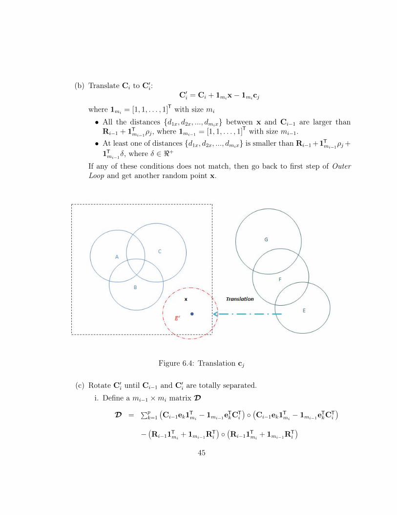
(b) Translate Ci to C0i:
C0i = Ci + 1mix� 1micj
where 1mi = [1, 1, . . . , 1]T with size mi
• All the distances {d1x, d2x, ..., dmix} between x and Ci�1
are larger thanRi�1
+ 1Tmi�1⇢j, where 1mi�1 = [1, 1, . . . , 1]T with size mi�1
.• At least one of distances {d
1x, d2x, ..., dmix} is smaller than Ri�1
+1Tmi�1⇢j+
1Tmi�1�, where � 2 <+
If any of these conditions does not match, then go back to first step of OuterLoop and get another random point x.
Figure 6.4: Translation cj
(c) Rotate C0i until Ci�1
and C0i are totally separated.
i. Define a mi�1
⇥mi matrix D
D =
Ppk=1
ÄCi�1
ek1Tmi� 1mi�1e
TkC
Ti
ä�ÄCi�1
ek1Tmi� 1mi�1e
TkC
Ti
ä
�ÄRi�1
1Tmi+ 1mi�1R
Ti
ä�ÄRi�1
1Tmi+ 1mi�1R
Ti
ä
45

where ek is a p-dimension standard basis, ek = [0, . . . , 1, . . . , 0]T only the kth element is 1.
ii. if (all elements in D are equale or larger than 0)Return C0
i
Figure 6.5: Translation
In Figure 6.5, not all elements in D are equale or larger than 0. Hence, weneed to do rotation until they are totally separated.
iii. else
• Inner Loop: ✓ = ⇡18
, 2⇡18
, . . . , 2⇡
• – C0i C0
i ⇥R⇤ for p = 2
R =
ñcos(✓) � sin(✓)sin(✓) cos(✓)
ô
46

⇤ for p =3
R =
2
641 0 0
0 cos(✓1
) � sin(✓1
)
0 sin(✓1
) cos(✓1
)
3
75
2
64cos(✓
2
) 0 sin(✓2
)
0 1 0
� sin(✓1
) 0 cos(✓2
)
3
75
2
64cos(✓
3
) � sin(✓3
) 0
sin(✓3
) cos(✓3
) 0
0 0 1
3
75
✓1
, ✓2
and ✓3
are not necessarily equal. For simplify, we can set✓1
= ✓2
= ✓3
= ✓
– Caculate D– if (all elements in D are equale or larger than 0) then break the
Inner Loop and return C0i
else ✓ ✓ + ⇡18
and repeat the Inner Loop• If ✓ = 2⇡ and D still doesn’t meet the conditions, then go back to
random point selection and pick a new x
47

Figure 6.6: Rotation
(d) Ci = [CTi�1
,C0iT]
T
(e) i i+ 1
3. Return C = C⌘ and C is final layout with all united groups.
48

Chapter 7
Examples
Figure 7.1 is an example of factor data on human encountering with great white sharks.The data is collected by Doctor Pierre-Jerome Bergeron [5]. In this example, it shows therelationship among nationality, time and fatality.
Figure 7.1: sharks data frame
Here, the supplementary sets of “AM”, “Australia and USA”, “Fatality” are “PM”, “oth-
49

ers”, “Survive”, respectively. So, any disjoint parts either fall into sets or supplementarysets. The stress of this example is 0.06922327.
Fifteen-ring data set with multiple groups S5
= {SA, SB, . . . , SP}, the input givendisjoint subsets I(S)?
4
with size s?I :
s?I = [s?A = 80, s?B = 50, s?C = 100, s?D = 100, s?E = 100, s?F = 40,
s?A,C = 30, s?A,D = 30, s?B,E = 30, s?A,E = 40, s?B,F = 10,
s?G = 60, s?H = 50, s?I = 100, s?J = 40, s?K = 50, s?L = 100,
s?M = 30, s?O = 50, s?P = 60, s?G,H = 20, s?K,L = 20, s?L,M = 20, s?O,P = 30]
P(S)?4
is the corresponding power set, any sets in the complement of I(S)?4
are ?. Figure7.2 shows the layout with stress 0.00014.
Figure 7.2: Multiple groups in one data set
50

However, not all data are suitable to be illustrated by area proportional Venn diagrams.For example, Figure 7.3 shows the size proportional Venn diagram of the data set in Figure1.4 (b).
Figure 7.3: Figure 1.4 (b) data set
The stress is 0.021 which should indicate a good quality Venn diagram. Nevertheless,we can only tell these five species share a large number of genes.
51

Chapter 8
Comparison with other Venn algorithms
We compare vennplot() with other popular approaches to the circular area-proportionalVenn algorithms venneuler() and venn.js().
We generate 100 instances of SP = {S1
, . . . , Sm} for each value of m = 3, 4, . . . , 8.For each SP generates its disjoint set s?P independently from U(0, 10). Compare results ofvennplot() with venneuler() and venn.js() on two criteria.
abs =NX
i
|b?i � s?i | stress =RSS
TSS
For each criterion will look at differences in results venneuler()�vennplot(), venn.js()�vennplot(). The larger this difference the more favoured is vennplot(). Figure 8.1 illus-trates the comparison with venneuler().
Figure 8.1: venneuler()- vennplot(), abs and stress
52

The abs of vennplot() is better after four circles, the stress is worse but comparable.We may also interested in how well the fit of each way intersection.
stress(k) =P
i2k�way br2iPi2k�way s2i
m is the highest order and 1 k m � 1 (when k = m, s?1...m = s
1...m); stress(k) is thecorresponding stress and comparison is shown in Figure 8.2.
Figure 8.2: venneuler() - vennplot(), stress(k), where 1 k m� 1
We can find vennplot() does better on the fit of stress(k), from three circles to eightcircles. However, if vennplot() did well on all intersections but bad in stress, whichshould indicate we fit really poor on s
1...m and the poor s1...m explodes up the stress.
Figure 8.3 illustrates the comparison of stress(m).
53

Figure 8.3: venneuler()- vennplot(), stress(m)
However, sometimes, people may also interested in the fit of total size, rather thandisjoint part. This can be captured by fitting the linear model:
bP = sP� + r
criteria stress is defined as � and the boxplot shows the comparison with venneuler(),given the random generation data set.
� =
brTbr
bPTbP
54

Figure 8.4: venneuler()- vennplot(), �
Since we cannot grab the centres and radii from javascript, we implement Frederick-son’s algorithm in R (suppose venn.js() is totally based on his algorithm on his website[18]), use random initial configuration as he did. Figure 8.5 shows the comparison on twocriteria with random generated data sets (the same as before).
Figure 8.5: venn.js() - vennplot(), abs and stress
The boxplot of abs are roughly symmetric around zero, which means they should bevery similar based on this criteria; stress is slightly better (that is because after mini-mizing 2.5, we import � to minimize stress). Frederickson did improve performance on
55

possible configurations, however, based on some impossible point configurations (like whatwe randomly generated), it may not surpass venneuler().
However, if there are multiple groups in one data set, the “three step rule” of vennplot(),divide, conquer and unite could really improve the performance. For example, Figure 8.6shows the layout of I(S)?
4
by venneuler() with stress 0.37. We can also generate eachdata set 100 times which contains two to five groups. In each group, circles vary from oneto five (if the maximum circle is over five, after four groups, venneuler() is more likely toterminate). Figure 8.7 illustrates the comparison.
Figure 8.6: For set I(S)?4
56

Figure 8.7: venneuler()- vennplot(), stress multiple groups
For venn.js(), if the stress of vennplot() is smaller in a single group, it would notperform worse in multiple groups.
For Wilkinson’s algorithm, the steepest descent, equation 2.3 has a problem: if theinitial configurations of balls (for example, bi and bj) are totally overlaid with each other,then, this steepest descent for ci and cj would be zero, thus bi and bj could be hardto separate. An example is S
5
= {SA, SB, SC , SD}, the disjoint subsets I(S)?5
with sizes?I = [s?A = 3, s?B = 3, s?C = 10, s?D = 10, s?AB = 2], P(S)?
5
is the corresponding power setand any sets in P(S)?
5
\ I(S)?5
are ?. Figure 8.8 shows the initial configuration and finallayout of venneuler().
57

(a) (b)
Figure 8.8: (a) is the initial configuration and (b) is the final one
For “Constrained MDS” (Frederickson’s algorithm), the main problem is that equation2.7 only focuses on the two way intersection but does not consider higher way intersections.Thus, he priorities to one way and two way intersections.
Except venneuler() and venn.js(), there is another good R function eulerr() withsimilar generalized Venn algorithms. The function is also based on Wilkinson and Fred-erickson’s algorithm, but with different optimizers. Also worth noting, in eulerr(), radiiare not fixed and taken as an optimizer. This behavior can largely decrease the abs andstress, Figure 8.9.
Figure 8.9: eulerr() - vennplot()
However, it will sacrifice the fit of other intersections, shown in Figure 8.10 and Fig-
58

ure 8.11. Sometimes, too many parameters can lead the program to fail providing Venndiagrams (like I(S)?
4
) [26].
Figure 8.10: eulerr() - vennplot(), �
59

Figure 8.11: eulerr() - vennplot(), stress(k) where 1 k m� 1
60

Figure 8.12: eulerr() - vennplot(), stress(m)
The experiment of multiple groups comparison is much more likely to terminate byeulerr(), hence we do not show the comparison.
61

Chapter 9
Discussion
Wilkinson’s algorithm tends to give disjoint areas the same weight. Hold radii fixed andmove centres. Frederickson’s algorithm starts from distances with noticing the subsets anddisjoint circles, and then, turns this problem (area proportional Venn diagram fit) into amultiple dimensional scaling minimizing problem. Our algorithm tries to balance two ofthem, seeking the minimum “MDS” and capturing a fine structure. Moreover, our modelis the first one with noting groups automatically. The layout is impressive when there aremultiple groups in one Venn diagram. The three-dimensional Venn diagrams can providea nice visualization in case two dimensional Venn diagrams fail (like Figure 1.4 (a) ).
For these three criteria ( , abs and stress), they can be taken as a reference, butnot truth. The criteria may be good for some configurations, but for real data, alltests may fail to reconstruct ( 10%). And this criteria is not bounded, if any disjointareas overlay a tiny bit, can go to 1. abs and stress are bounded criteria, however,sometimes, they are not trustworthy either. There is an example on Frederickson’s website,where S
6
= {SA, SB}, the power set P(S)?6
with size s?P = [s?A = 98, s?B = 48, s?AB = 0].Figure 9.1 shows the layout of venneuler(). The abs and stress are 0.0137, 7.3 ⇥ 10
�5,which should indicate a good fit. However, we can find the there is an intersection betweenSA and SB, very small but noteworthy [19]. So, this gives us a warning, a good Venndiagram must have a very small criteria, but a small criteria does not indicate a good Venndiagram.
62

Figure 9.1: small stress but fit bad
63

Chapter 10
Appendix
• Line Search [6] for finding �:
�(n)+
�(n) +�
�(n)� �(n) ��
where � 2 <+, a small step size. Fixing �(n)+
and �(n)� to compute stress(�(n)+
) andstress(�(n)� ).
– if(min(stress(�+
), stress(��), stress(�(n))) = stress(�(n)))Return C C(n)
– else
1. if (min(stress(�+
), stress(��), stress(�(n))) = stress(�+
)) which meansshrinkage can decrease stress. Thus,
�(n) �+
and stress(�(n)) stress(�+
)
(a) update ��(n+1) �(n) +�
(b) update count nn n+ 1
(c) Fixing �(n) and compute stress(�(n))
(d) Repeat i to iii until stress(�(n�1)
) stress(�(n))
64

(e) Return C C(n�1) and stress = stress(�(n�1)
)
2. else which means expansion can decrease stress. Thus,
�(n) ��
And � can be updated as follows:
�(n+1) �(n) ��
The rest procedure is similar with (a). ii to v.
• Nelder Mead Algorithm [31] for finding µ:
1. Setµ(n)+
µ(n)+�
µ(n)++
�(n) + 2�
where � 2 <+ and µ can be defined as:
µ(n) [µ(n), µ(n)+
, µ(n)++
]
Thus we can get corresponding estimated distance matrix. Fixing �(1), stressis:
stress(n) = [stress(�(1);µ(n)), stress(�(1);µ(n)
+
), stress(�(1);µ(n)++
)]
2. The rest procedure is similar with “Nelder Mead Algorithm [31] for finding �”:fix �(1), do Loop but replace �(n) to µ(n)
3. Returnµ =
P(µ(n)
)
3
and corresponding distance [
bdij]
65

Bibliography
[1] Pax6 gene, July 2014.
[2] D. Ashlock, E.Y. Kim, and L. Guo. Multi-clustering: Avoiding the natural shape ofunderlying metrics. Smart Engineering System Design: Neural Networks, Evolution-ary Programming, and Artificial Life, 15:453–461, 2005.
[3] Vic Barnett, editor. Interpreting multivariate data. John Wiley & Sons, 1981.
[4] Margaret E. Baron. A Note on the Historical Development of Logic Diagrams: Leibniz,Euler and Venn. The Mathematical Gazette, 1969.
[5] Pierre Jerome Bergeron. sharkattackinfo.com, 2017.
[6] M. J Box, D Davies, and W. H Swann. Non-linear optimization techniques. Edinburgh:Published for Imperial Chemical Industries Ltd by Oliver Boyd, 1969, 1969.
[7] Allyson L. Byrd, Clay Deming, Sara K. B. Cassidy, Oliver J. Harrison, Weng-IanNg, Sean Conlan, NISC Comparative Sequencing Program, Yasmine Belkaid, Julia A.Segre, and Heidi H. Kong. Staphylococcus aureus and Staphylococcus epidermidisstrain diversity underlying pediatric atopic dermatitis. Science, 2017.
[8] Hanbo Chen and Paul C Boutros. Venndiagram: a package for the generation ofhighly-customizable Venn and Euler diagrams in R. BMC Bioinformatics, 2011.
[9] W.H. Cherry and R.W. Oldford. Picturing Probability: the poverty of venn diagrams,the richness of Eikosograms. (unpublished manuscript), 2003.
[10] S. Chow and P. Rodgers. Constructing area-proportional Venn and Euler diagramswith three circles. Euler Diagrams Workshop, 2005.
66

[11] S. Chow and F. Ruskey. Drawing Area-Proportional Venn and Euler Diagrams. GraphDrawing, 2003.
[12] William S. Cleveland and Robert McGill. Graphical Perception: Theory, Experi-mentation, and Application to the Development of Graphical Methods . AmericanStatistical Association, 1984.
[13] William S. Cleveland and Robert McGill. Graphical Perception and Graphical Meth-ods for Analyzing Scientific Data. Science, 1985.
[14] William S. Cleveland and Robert McGill. Graphical Perception : The Visual Decodingof Quantitative Information on Graphical Displays of Data . Royal Statistical Society,1987.
[15] L. Euler. Lettres a Une Princesse d’Allemagne, volume 2. Charpentier, 1843.
[16] Leonhard Euler. Letters cii through cviii. In D. Brewster, editor, Letters of Euler ondifferent subjects in Natural Philosophy addressed to a German Princess. (Translatedfrom Lettres à une Princesse d’Allemagne), volume I, pages 337–366. Harper andBrothers, New York, 1840 (1761 original).
[17] Ben Frederickson. Calculating the intersection area of 3+ circles, 2013.
[18] Ben Frederickson. A better algorithm for area proportional Venn and Euler diagrams,2015.
[19] Ben Frederickson. Comparison with venneuler, 2015.
[20] John Hopcroft and Robert Tarjan. Algorithm 447: efficient algorithms for graphmanipulation. Communications of the ACM, 1973.
[21] Catherine Q. Howe and Dale Purves. Natural-scene geometry predicts the perceptionof angles and line orientation. Proceedings of the National Academy of Sciences of theUnited States of America, 102(4):1228–1233, 2005.
[22] C.B. Hurley and R.W. Oldford. PairViz: Visualization using Eulerian tours andHamiltonian decompositions, 2011. R package version 1.2.1.
[23] Paul Jaccard. Distribution de la Flore Alpine dans le Bassin des Dranses et dansquelques regions voisines. Bulletin de la Socieete vaudoise des sciences naturelles,1901.
67

[24] H. A. Kestler, A. Muller, J. M. Kraus, M. Buchholz, T. M. Gress, H. Liu, D. W. Kane,B. Zeeberg, and J. N. Weinstein. VennMaster: Area proportional euler diagrams forfunctional GO analysis of microarrays. BMC Bioinformatics, 2008.
[25] Ravi Kumar, Jasmine Novak, Prabhakar Raghavan, and Andrew Tomkins. Structureand evolution of blogspace. Structure and evolution of blogspace, 2004.
[26] Johan Larsson. An introduction to eulerr, 2017.
[27] Daniel P. LePage, Jason A. Metcalf, Sarah R. Bordenstein, Jungmin On, Jessamyn I.Perlmutter, J. Dylan Shropshire, Emily M. Layton, Lisa J. Funkhouser-Jones, John F.Beckmann, and Seth R. Bordenstein. Prophage WO genes recapitulate and enhanceWolbachia-induced cytoplasmic incompatibility. Nature, 2017.
[28] R Beau Lotto and Dale Purves. The empirical basis of color perception. Consciousnessand Cognition, 11(4):609 – 629, 2002.
[29] Luana Micallef and Peter Rodgers. (eulerape: Drawing area-proportional 3-venn dia-grams using ellipses. PLOS.
[30] B. Minaei-bidgoli, A. Topchy, and W. F. Punch. A comparison of resampling methodsfor clustering ensembles. In the International Conference on Artificial Intelligence,pages 939 – 945, 2004.
[31] J. A. Nelder and R. Mead. A simplex method for function minimization. The ComputerJournal, 1969.
[32] R. Wayne Oldford. Constraint-oriented programming with application to statisticalgraphics. In Bulletin of the International Statistical Institute, volume 54, pages IP–21/3 1–18, Cairo, Egypt, 1991. International Statistical Institute.
[33] R. Wayne Oldford. Self-calibrating quantile–quantile plots. The American Statistician,70(1):74–90, February 2016.
[34] Richmond Wayne Oldford. qqtest: Self calibrating quantile quantile plots for visualtesting, 2014. R package version 1.1.1.
[35] R.W. Oldford. Mental models and interactive statistics: Design principles. In Comput-ing Science and Statistics, volume 31, pages 254–262. Interface Foundation of NorthAmerica, 1999.
68

[36] D.J. Parkhurst and E. Niebur. Scene content selected by active vision. Spatial Vision,16:125–154, 2003.
[37] E Polak and G Ribiere. Note sur la convergence de méthodes de directions conjuguées.Mathematical Modelling and Numerical Analysis, 1969.
[38] Adam Rahman and Wayne Oldford. Euclidean distance matrix completion and pointconfigurations from the minimal spanning tree. (unpublished manuscript), 2016.
[39] Frank Ruskey and Mark Weston. A survey of venn diagrams. THE ELECTRONICJOURNAL OF COMBINATORICSl, 2005.
[40] Jonathan R Shewchuk. Technical report. An Introduction to the Conjugate GradientMethod Without the Agonizing Pain, 1994.
[41] Elizabeth S. A. Sollars, Andrea L. Harper, Laura J. Kelly, Christine M. Sambles,Ricardo H. Ramirez-Gonzalez, David Swarbreck, Gemy Kaithakottil, Endymion D.Cooper, Cristobal Uauy, Lenka Havlickova, Gemma Worswick, David J. Studholme,Jasmin Zohren, Deborah L. Salmon, Bernardo J. Clavijo, Yi Li, Zhesi He, AlisonFellgett, Lea Vig McKinney, Lene Rostgaard Nielsen, Gerry C. Douglas, Erik DahlKjaer, J. Allan Downie, and David Boshier. Genome sequence and genetic diversityof European ash trees. Nature, 2016.
[42] S.S. Stevens. On the psychophysical law. Psychological Review, 1957.
[43] W. Torgerson. Multidimensional scaling: I. theory and method. Psychometrika, 1952.
[44] Antony Unwin, Martin Theus, and Heike Hofmann. Graphics of large datasets: visu-alizing a million. Springer, 2006.
[45] John Venn. On the diagrammatic and mechanical representation of propositions andreasonings. The London, Edinburgh, and Dublin Philosophical Magazine and Journalof Science, X(5):1–18, July 1880.
[46] A. Weingessel, E. Dimitriadou, and K. Hornik. An ensemble method for clustering.In Conference of Directions in Statistical Computing, 2003.
[47] Wikipedia. List of alternative names for the human species.
[48] Leland Wilkinson. Exact and approximate area-proportional circular Venn and Eulerdiagrams. IEEE Trans Vis Comput Graph, 2012.
69

[49] Dongsheng Zhang, Mengchao Yu, Peng Hu, Sihua Peng, Yimeng Liu, Weiwen Li,Congcong Wang, Shunping He, Wanying Zhai, Qianghua Xu, and Liangbiao Chen.Genetic Adaptation of Schizothoracine Fish to the Phased Uplifting of the Qinghai -Tibetan Plateau. Genetics, 2017.
70