size at first maturity and recruitment into egg production
TRANSCRIPT

Size at first maturity andrecruitment into egg production
of southern bluefin tuna
Mathematical& Information
Sciences
��������������������
���������
DE
PAR
TEMEN KELAUTAN DAN
PERIK
AN
Tim Davis
Jessica Farley
Mark Bravington
Retno Andamari
Project No. 1999/106
Final Report

Size at first maturity and recruitment into egg production of southern bluefin tuna. Bibliography. Includes index. ISBN 1 876996 33 1. 1. Bluefin tuna - Size - Australia, Southern. 2. Bluefin tuna - Spawning - Australia, Southern. 3. Bluefin tuna - Fertility - Australia, Southern. I. Davis, Tim L. O. (Tim Lionel Ormandy). II. CSIRO. Marine Research. 639.277830994

FRDC 1996/106 Final Report
TABLE OF CONTENTS
1. Non-technical Summary............................................................................1 2. Acknowledgments .....................................................................................5 3. Background...............................................................................................5 4. Need .........................................................................................................6 5. Objectives .................................................................................................6 6. Methods ....................................................................................................6
6.1 Biological Sampling of SBT..........................................................................6 6.2 Laboratory Processing and Histology of Ovaries..........................................7 6.3 Histological Classification of Ovaries ...........................................................8 6.4 Fecundity Estimation .....................................................................................9 6.5 Age Determination.........................................................................................9 6.6 Longline Catch/Depth Monitoring ................................................................9
7. Results on Spawning and Effects of Depth of Fishing.............................10 7.1 Biological Data Collected............................................................................10 7.2 Longline Catch/Depth Monitoring ..............................................................12 7.3 Spawning Season .........................................................................................15
7.3.1 Length Effects....................................................................................15 7.3.2 Age Effects ........................................................................................17
7.4 Spawning .....................................................................................................18 7.4.1 Spawning Fraction.............................................................................19 7.4.2 Atresia................................................................................................21 7.4.3 Spawning Frequency .........................................................................23 7.4.4 Effects of Length on Atresia and Spawning Frequency ....................24 7.4.5 Effects Of Age On Atresia And Spawning Frequency......................26 7.4.6 Effects of Bigeye Index on atresia and spawning frequency.............27 7.4.7 Spawning Duration ............................................................................29
7.5 Batch Fecundity ...........................................................................................31 7.6 Conclusions on Spawning and Effects of Depth of Fishing ........................34
8. Population Egg Production......................................................................37 8.1 Estimating Spawning Rates by Depth .........................................................39 8.2 Estimating Time Spent on Grounds.............................................................40 8.3 Estimating Relative Average Individual Spawning Events.........................41
8.3.1 Confidence Intervals and Effect of Assessment Choice on RAISE ..42 8.4 Effects of Assumptions About f -at-depth on RAISE................................44 8.5 Batch Fecundity ...........................................................................................45 8.6 Forming a time series of relative egg production ........................................47
8.6.1 Sensitivity to Model Assumptions.....................................................48 8.7 Comparison With SSB Series ......................................................................50
9. Conclusions.............................................................................................51 10. Benefits .................................................................................................53 11. Planned Outcomes................................................................................53 12. Further Development ............................................................................53
12.1 Further data requirements ..........................................................................53 12.1.1 Histology .........................................................................................53 12.1.2 Biological Data on Depth Distribution............................................54
12.2 Further Integration with Assessment .........................................................55 12.2.1 Reducing circularity ........................................................................55
i

FRDC 1996/106 Final Report
12.2.2 Including Length-Depth Modeling..................................................55 13. References ........................................................................................... 56 14. Intellectual property .............................................................................. 58 15. Staff ...................................................................................................... 58 16. List of appendices................................................................................. 58
LIST OF TABLES
Table 7.1.1. Number of biological parameters determined on SBT whose ovaries were sampled in each spawning season............................................................10
Table 7.2.1. Settled depths (m) of longline at hook positions on consecutive sets in March 2000 for a 13 hooks between floats configuration (hook 1 and 13 occupy the same depth position on each side of the catenary). Hook position 1/13 and 2/12 were not occupied in all sets.....................................................................13
Table 7.2.2. Temperature (ºC) at settled depths of longline at hook positions on consecutive sets in March 2000 for a 13 hooks between floats configuration. 13
Table 7.2.3. Settled depths (m) of longline at hook positions on consecutive sets in October-November 2001 for a 14 hooks between floats configuration. ..........14
Table 7.4.1. Number of samples used to determine fraction of ovaries with atresia by month and spawning season. The year of the spawning season is defined by January..............................................................................................................22
Table 8.1.1. Percentage at “depth”, within length class and spawning status. Depth proxied by bigeye index. “About to spawn” means “with ovaries that have migratory-nucleus or hydrated eggs”. ..............................................................40
Table 8.1.2. Percentage of fish with migratory-nucleus or hydrated oocytes by length and depth. Small numbers are sample sizes. ....................................................40
Table 8.3.1. Estimated per capita number of spawning events, relative to 190 cm fish. Assumes equal f across depths. Assessment OM9RR5....................................43
Table 8.3.2. Estimated per capita number of spawning events, relative to 190 cm fish. Assumes equal f across depths. Assessment PM2RR8. ...................................43
Table 8.5.1. Estimated batch fecundities, relative to a 190 cm fish .........................46 Table 8.6.1. Relative egg production per capita by length, combining RAISE and
batch fecundity. ................................................................................................47 Table 9.1. Point estimates for parameters in the egg production model relative to a
190 cm fish .......................................................................................................52 LIST OF FIGURES
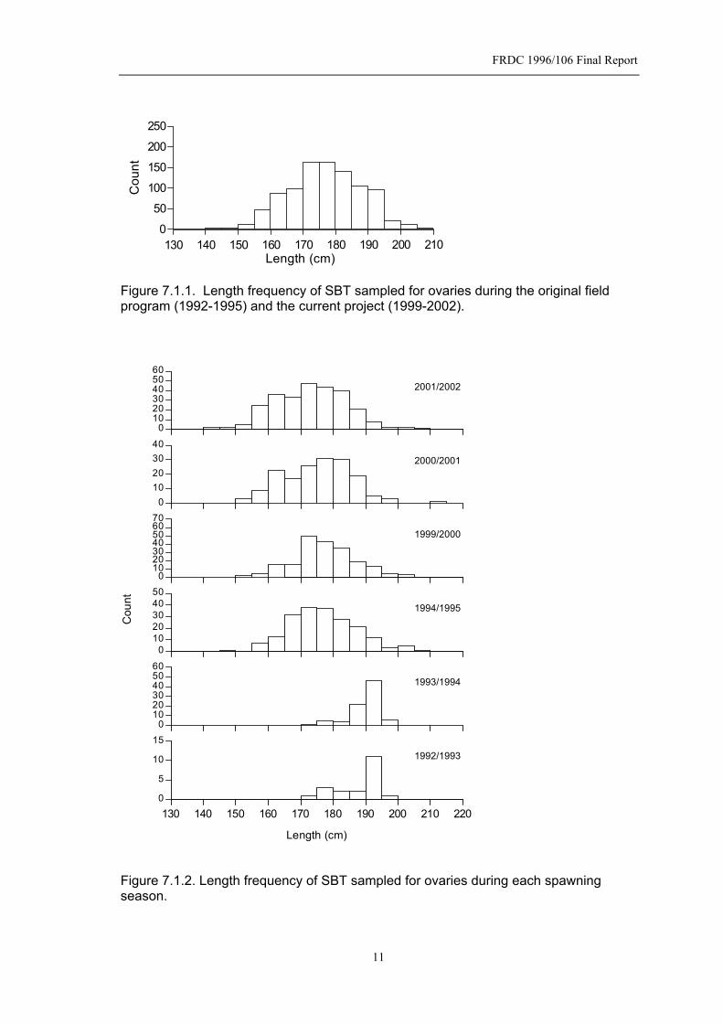
Figure 7.1.1. Length frequency of SBT sampled for ovaries during the original field program (1992-1995) and the current project (1999-2002). ............................11
Figure 7.1.2. Length frequency of SBT sampled for ovaries during each spawning season................................................................................................................11
Figure 7.1.3. Age distribution of SBT (2 year intervals) sampled for ovaries during the current project (1999-2002)........................................................................12
ii

FRDC 1996/106 Final Report
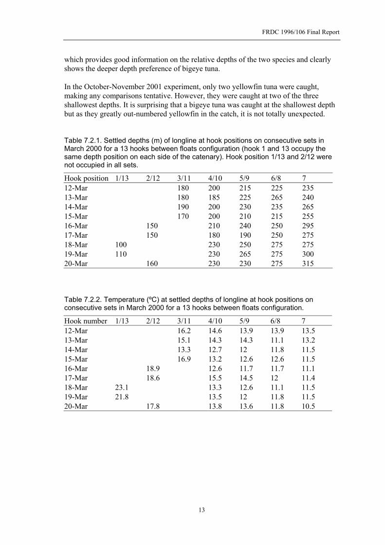
Figure 7.2.1. Depth and temperature at which bigeye and yellowfin tuna were caught during the two longline fishing performance experiments in March 2000 and October-November 2001. .................................................................................14
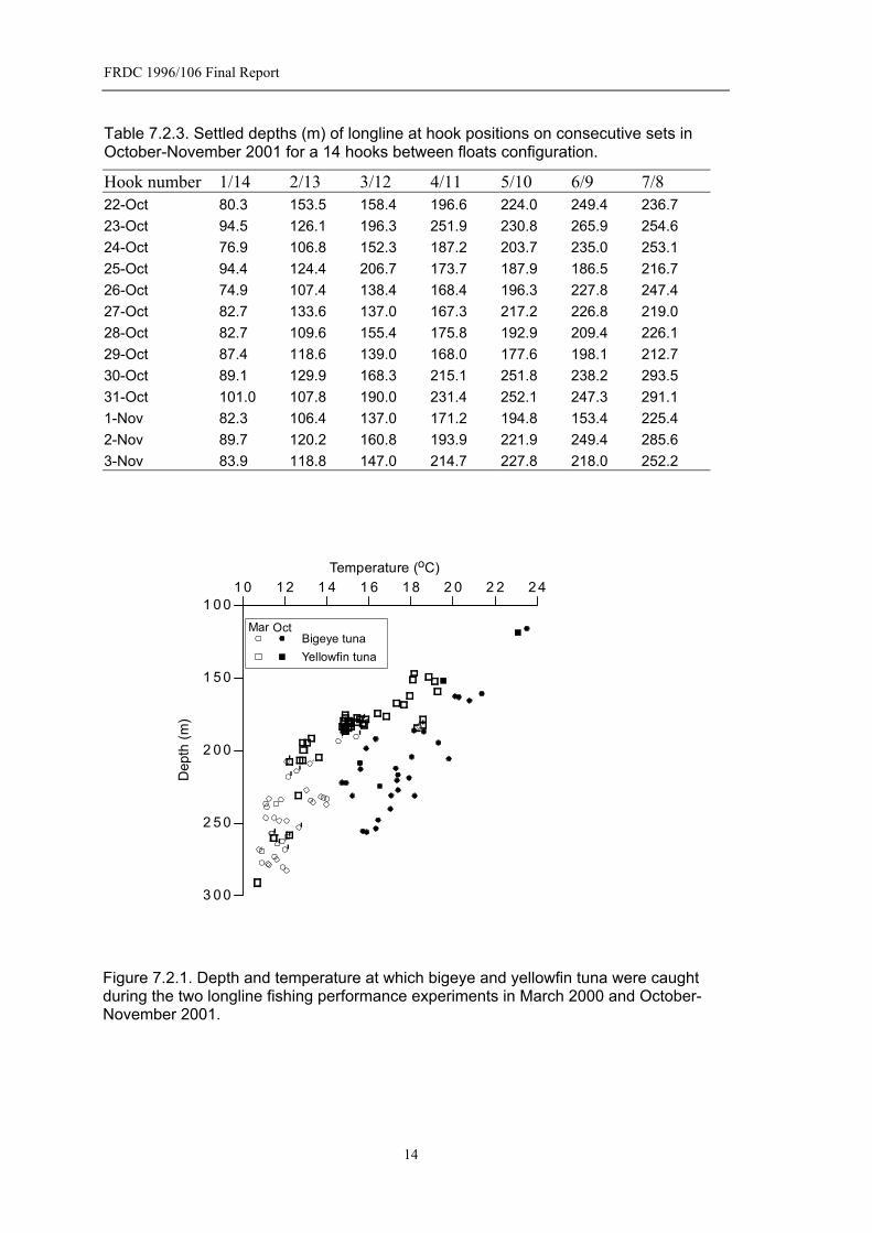
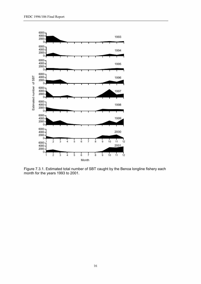
Figure 7.3.1. Estimated total number of SBT caught by the Benoa longline fishery each month for the years 1993 to 2001.............................................................16
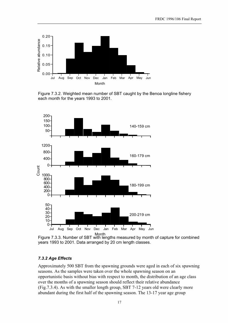
Figure 7.3.2. Weighted mean number of SBT caught by the Benoa longline fishery each month for the years 1993 to 2001.............................................................17
Figure 7.3.3. Number of SBT with lengths measured by month of capture for combined years 1993 to 2001. Data arranged by 20 cm length classes. ..........17
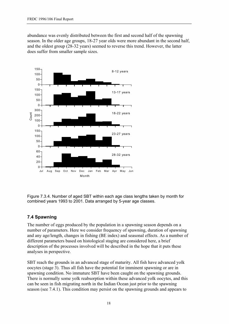
Figure 7.3.4. Number of aged SBT within each age class lengths taken by month for combined years 1993 to 2001. Data arranged by 5-year age classes................18
Figure 7.4.1. Fraction of spawning SBT by spawning season. The year of the spawning season is defined by January. Sample sizes are indicated and vertical bars represent 95% confidence limits of the mean. ..........................................19
Figure 7.4.2. Fraction of spawning SBT by month for the years 1992-1995 (o) and 1999-2002 (x). The zero September fraction was based on three fish. ............20
Figure 7.4.3. Fraction of spawning SBT by month for all years combined. Sample sizes are indicated and vertical bars represent 95% confidence limits of the mean..................................................................................................................20
Figure 7.4.4. Fraction of SBT ovaries with <10% atresia by spawning season. The year of the spawning season is defined by January. Sample sizes are indicated and vertical bars represent 95% confidence limits of the mean. ......................21
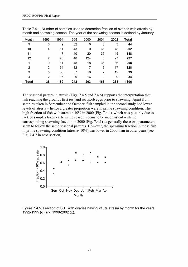
Figure 7.4.5. Fraction of SBT with ovaries having <10% atresia by month for the years 1992-1995 (o) and 1999-2002 (x). ..........................................................22
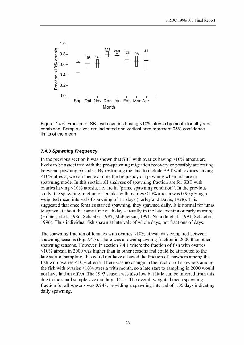
Figure 7.4.6. Fraction of SBT with ovaries having <10% atresia by month for all years combined. Sample sizes are indicated and vertical bars represent 95% confidence limits of the mean. ..........................................................................23
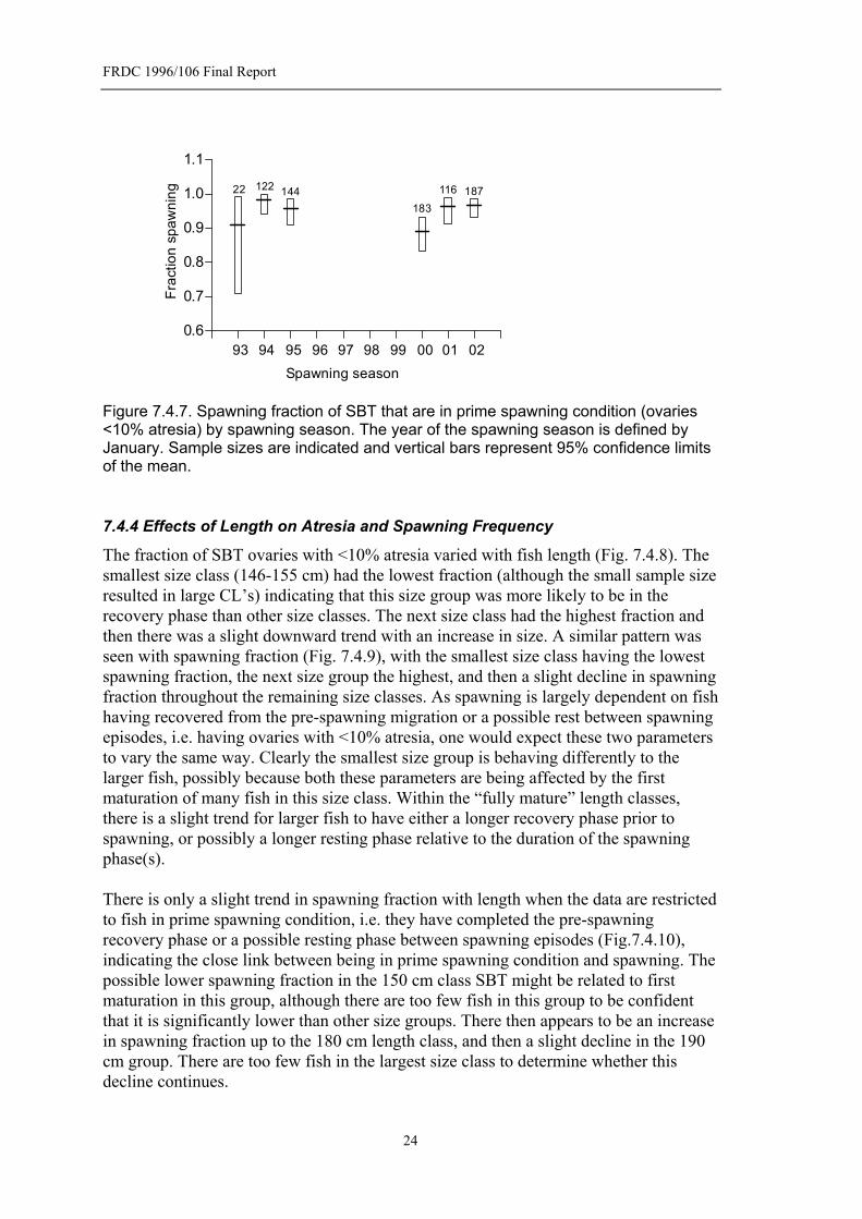
Figure 7.4.7. Spawning fraction of SBT that are in prime spawning condition (ovaries <10% atresia) by spawning season. The year of the spawning season is defined by January. Sample sizes are indicated and vertical bars represent 95% confidence limits of the mean. ..........................................................................24
Figure 7.4.8. Fraction of SBT ovaries in prime spawning condition (<10% atresia) by 10 cm length class. Sample sizes are indicated and vertical bars represent 95% confidence limits of the mean. ..........................................................................25
Figure 7.4.9. Spawning fraction of SBT by 10 cm length class. Sample sizes are indicated and vertical bars represent 95% confidence limits of the mean........25
Figure 7.4.10. Spawning fraction of SBT that are in prime spawning condition (ovaries <10% atresia) by 10 cm length class. Sample sizes are indicated and vertical bars represent 95% confidence limits of the mean. .............................25
Figure 7.4.11. Fraction of SBT ovaries with <10% atresia by 5 year interval age groups. Sample sizes are indicated and vertical bars represent 95% confidence limits of the mean. ............................................................................................26
Figure 7.4.12. Spawning fraction of SBT by 5 year interval age groups. Sample sizes are indicated and vertical bars represent 95% confidence limits of the mean..27
Figure 7.4.13. Spawning fraction of SBT that are in prime spawning condition (ovaries <10% atresia) by 5 year interval age groups. Sample sizes are indicated and vertical bars represent 95% confidence limits of the mean. ......................27
iii
FRDC 1996/106 Final Report
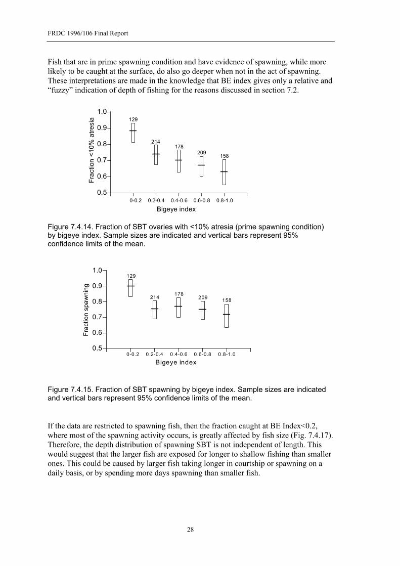
Figure 7.4.14. Fraction of SBT ovaries with <10% atresia (prime spawning condition) by bigeye index. Sample sizes are indicated and vertical bars represent 95% confidence limits of the mean...................................................28
Figure 7.4.15. Fraction of SBT spawning by bigeye index. Sample sizes are indicated and vertical bars represent 95% confidence limits of the mean. ......................28
Figure 7.4.16. Spawning fraction of SBT that are in prime spawning condition (<10% atresia) by bigeye index. Sample sizes are indicated and vertical bars represent 95% confidence limits of the mean...................................................29
Figure 7.4.17. Fraction of each size class of spawning SBT that were caught at BE Index<0.2 (the shallowest sets). .......................................................................29
Figure 7.4.18. Relation between spawning duration (number of sequential days spawning) and length based on a binomial GLM. 95% confidence limits of the estimate are shown............................................................................................30
Figure 7.5.1. Batch fecundity of SBT by length.......................................................31 Figure 7.5.2. Batch fecundity of SBT by body weight.............................................32 Figure 7.5.3. Batch fecundity of SBT by age. Data separated into three length
classes. ..............................................................................................................32 Figure 7.5.4. Batch fecundity by ovary weight. Data separated into three length
classes. ..............................................................................................................33 Figure 7.5.5. Ovary weight by fish length. Data grouped by hydrated oocyte stage
(pe-spawning) and advanced yolk with early POFs (immediately after spawning) to examine the effects of hydration on ovary weight......................33
Figure 7.5.6. Diameter of hydrated oocytes by ovary weight. Effect of stage of hydration on weight of ovary. Data grouped by 20 cm length class. ...............33
Figure 8.2.1. Overall fit of the length-depth model..................................................42 Figure 8.4.1. Contours of relative estimated per capita spawning events. Assessment
OM9RR5. .........................................................................................................44 Figure 8.5.1. Ovary weight versus fish length. Small dots/thin line are ovaries at
stage 3 (advanced yolked oocytes) with stage 1 and 2 POFs and solid/thick line are ovaries at stage 5 (hydrated oocytes) and without stage 1 POFs. Regression lines have different intercepts but identical slopes...........................................46
Figure 8.6.1. Relative individual SSB (dotted) and egg production (dashed) by age...........................................................................................................................48
Figure 8.6.2. Time series of total egg production. Dashed line; “optimistic” (OM9RR5). Dotted line; “pessimistic” (PM2RR8). Both lines normalized to have mean 1. 1994 df set equal at all depths. ....................................................48
Figure 8.6.3. Total egg production relative to mean. Dashed line; low f on shallow. Dotted line; low f on deep..............................................................................49
Figure 8.6.4. Total egg production relative to mean. Solid line uses point estimate of 2.47: dotted and dashed lines are lower and upper 95% confidence limits (~2.1 and ~2.0). Assessment OM9RR5, equal f across depths. ...............................49
Figure 8.7.1. Comparison of spawning stock biomass and egg production series for assessment PM2RR8 (pessimistic). Lines are normalized to have mean 1. Equal f at depth is assumed. ........................................................................................50
iv
Figure 8.7.2. Comparison of spawning stock biomass and egg production series for assessment OM9RR5 (optimistic). Lines are normalized to have mean 1. Equal f at depth is assumed. ..........................................................................................51
FRDC 1996/106 Final Report
1. Non-technical Summary 1999/106 Size at first maturity and recruitment into egg production of southern bluefin tuna Principal Investigator: Tim Davis Address: CSIRO Marine Research
GPO Box 1538 Hobart TAS 7000
Telephone: 02 6232 5242 Fax: 02 6232 5012 Objectives: 1. Determine the mean size at first maturity of SBT on the spawning grounds. 2. Determine the relationship between spawning frequency and size. 3. Determine the relationship between batch fecundity and size. 4. Model the recruitment dynamics of population egg production. Outcomes Achieved: This study has provided new information on the spawning dynamics of SBT and this has enabled us to refine previous estimates of spawning parameters and investigate size/age and fisheries related trends in these parameters. With this increased understanding of spawning dynamics we have been able to determine size related changes in the key parameters needed to develop an egg production model for SBT. We have successfully produced an egg production model that uses information on spawning derived from histology, information on the temporal distribution of SBT by depth on the spawning ground, and information on numbers at length from a stock assessment. The resulting population egg production provides a greatly improved indicator of spawning stock biomass for use in stock assessment and prediction. The main benefits are likely to be in better predictions. Using spawning stock biomass as a proxy for spawning potential gives quite a different stock-recruitment relationship during a period of stock decline, than during the subsequent recovery. However, this artifact disappears if a better proxy for spawning potential, such as population egg production is used. Stock projections to examine medium to long term consequences of current catches on parental biomass and the probability of recovery to the 1980 levels depend on good information on the recruitment dynamics of population egg production. We have provided this, and as expected, the two orders of magnitude difference in the relative egg production of a 160 cm and 190 cm fish will have profound effects on how long it takes for the SBT population to recover to 1980 levels of egg production. These differences are amply large enough to warrant properly incorporating egg production into stock assessments to provide better stock predictions and improved information for managers.
1

FRDC 1996/106 Final Report
Non-technical Summary: This project was initiated to provide supplementary data on the reproductive dynamics of SBT following a baseline study in 1992-1995. The purpose was to increase our information and understanding of SBT spawning dynamics in order to determine annual egg production as a function of fish length. This information would then be used in stock assessments to provide a measure of total egg production, which would replace the current spawning stock biomass as the “stock” variable in stock-recruit modeling. Field collections were made over three spawning seasons starting from November 1999 to March 2002. In this project 640 ovaries of SBT were histologically staged to supplement the 475 collected previously in 1992-1995. Fecundity estimates were made on a further 16 fish. No age determinations were possible in the first field program as otoliths were not collected from fish that provided gonad samples. The age of almost half of the SBT sampled in the current study were aged, and importantly, catch details including bigeye index, were recorded for most SBT sampled. The bigeye index has been shown to be a proxy for fishing depth as it is based on the fraction of bigeye to yellowfin in a catch – the two species have differing depth preferences. From these additional samples we were able refine previous estimates of spawning parameters and investigate size/age and fisheries related trends in these parameters. The spawning season starts in September and continues to April. There are generally two peaks in abundance of SBT on the spawning ground, one in October and one in January. The size of these peaks varies from year to year. SBT arriving on the spawning ground usually require a period of recovery before spawning commences. SBT south of and in transit to the spawning grounds have a high incidence of atresia – a process by which yolk is reabsorbed from eggs, possibly to rationalize the supply of yolked eggs and to reorganise the ovary before the start of spawning. SBT arrive on the spawning ground in this condition or just recovering from it. Once SBT have completed the pre-spawning phase and atresia is more or less complete, they are in prime spawning condition and then spawn each day. We observed a trend for an increase in the number of consecutive daily spawnings with fish size, with 150 cm fish spawning on about 3.6 consecutive days and 190 cm fish spawning on about 6.8 consecutive days. It is possible that larger fish might have more than one spawning episode and rest between spawning episodes. We do not have direct information on how long individual SBT remain on the spawning grounds. This type of information is best obtained by the use of archival tagging, and so far no archival tags have been recovered from SBT that have visited the spawning grounds. The results of investigations on the depth of longline fishing using temperature-depth recorders generally confirmed that bigeye tuna tended to be caught at deeper hook positions than yellowfin tuna. An index based on the proportion of bigeye tuna in longline catches (BE Index) provided an indication of the depth of capture, however because of the imprecision inherent in the relationship between longline fishing depth (and how it is estimated) and catch, it could only be used to look for trends in data. Despite its looseness as a proxy for depth, the BE Index indicated how markedly the depth of fishing can affect estimation of parameters defining spawning dynamics.
2

FRDC 1996/106 Final Report
Both the fraction of females in prime spawning condition and the fraction spawning is much higher at a low BE index (surface catches) than at a high BE index. The greatest difference occurs at the lowest BE Index where significantly higher fractions of SBT are in prime spawning condition and are spawning. It is this lowest BE Index that provides the “cleanest” proxy for depth as it will not be subject to problems of contamination by fishing at other depths. Some of the deeper hooks may catch fish before they settle or as they are being retrieved. The fraction of each size group of SBT that are caught at the surface increases with fish size. This means that larger SBT are exposed to surface fishing for longer than smaller fish. This suggests that the number of spawnings and/or the amount of time spent spawning or in courtship at the surface probably increases with fish size. Because depth affects spawning parameters, it is important that these effects are taken into account when developing a method to calculate total egg production. All objectives in this project were met, although some of these have not been presented explicitly as they were either an intermediate step in the population egg production model or had been replaced by a more relevant and improved parameter. The mean size at maturity of SBT on the spawning grounds (Objective 1) was not estimated explicitly as it was integrated in the “average availability” of length class on the spawning grounds. This term incorporates (i) the proportion mature at a particular length × (ii) the average duration of stay of mature fish of that length on the spawning ground. It provides the average relative duration a fish of a given length spends on the spawning ground. This term has the most profound effect on population egg production of all the parameters in the egg production model. Objective 2, the relationship between spawning frequency and size was determined from the histology data. Once fish start a spawning cycle on the spawning grounds they spawn daily, irrespective of size. However, they undergo a resting phase on arrival at the spawning grounds before starting spawning, and if they undergo more than one spawning cycle will rest between cycles. The relative proportion of time spent resting/recovering and time spent spawning also varied with size. This information was used in conjunction with information on the depth distribution by size to estimate the relative proportion of fish that would spawn every day by depth and length class. Both duration and depth integrated spawning frequency were then used to determine the relative average individual spawning events for a fish of a given size. The relationship between batch fecundity and size (Objective 3) was determined indirectly after it was found that direct fecundity estimates were (naturally) so highly variable that it would not be possible to ever obtain a sufficient number of estimates to give the precision required in an egg production model. Instead, we determined the relative batch fecundity based on the ovary weight difference between a fish about to spawn and one that had just completed the daily spawning event. Relative batch fecundity was consistent with the relationship between direct measurements of batch fecundity and size, however it could be estimated more precisely. The product of relative batch fecundity and relative average number of individual spawning events then provided relative egg production by size. The egg production model (Objective 4) uses numbers at length from a stock assessment to estimate the relative average duration a fish of a given length spends on
3

FRDC 1996/106 Final Report
the spawning ground (duration) and to generate a time series of total relative egg production. The choice of stock assessments will change the estimates of these parameters slightly. However, the differences in relative egg production with size are profound, regardless of which assessment of Kolody and Polacheck (2001) is used. There is a two orders of magnitude difference in the point estimates of relative egg production between a 160 cm and 190 cm fish for the most pessimistic assessment. This difference is only slightly less for the most optimistic assessment. This will have profound effects on the recovery of egg production by a population as 50% recruitment into population egg production is not reached until 17 years whereas 50% recruitment into the spawning stock biomass is reached at 11 years. These differences are amply large enough to warrant properly incorporating egg production into stock assessments. Further improvements to the precision of population egg production would result if more data could be obtained on the relative time at depth of any one length class. This would provide better information on relative fishing mortality at depth. This could be assessed accurately from archival tag data. Archival tag data would also allow direct estimation of duration on the spawning grounds. At a minimum, this would provide a useful consistency check on estimates of availability by age. More ambitiously, though, duration on grounds could be used to provide estimates of relative abundance by length that are effectively independent of the rest of the assessment. Assuming equal catchability for all sizes of fish present on the grounds at a particular depth, then the number of captures at that depth (relative across length classes) will be proportional to relative abundance of length classes, times the mean duration on the grounds. As well as helping to establish an unambiguous direct biological estimate of relative egg production, this would be of great value to the assessment itself. The development of a population egg production model provides a greatly improved indicator of spawning potential for use in stock assessment and prediction than the currently used spawning stock biomass. The differences are amply large enough to warrant properly incorporating egg production into stock assessments. The main benefits are likely to be in better stock predictions as the stock-recruitment relationship is genuinely based on spawning potential not just on biomass of the spawning stock. This will ultimately produce better management advice for managers of the SBT fishery. Keywords: Southern bluefin tuna, maturity, batch fecundity, spawning frequency, population egg production.
4
FRDC 1996/106 Final Report
2. Acknowledgments This research has depended largely on the efforts of staff from the Research Institute of Marine Fisheries and the Research Institute for Mariculture, Gondol in making biological collections of SBT samples at processing sites in Benoa, Bali, and histologically processing of ovaries and subsequent examination at Gondol. Dr Zafril Imran Azwar was the project leader in 1999/2000 before moving to a different department. Ibu Retno Andamari (Poppy) took over this role in 2000 and has made a major contribution in coordinating all Indonesian activities and supervising the histology and interpretation of gonad material. We are grateful to all the Indonesian staff that have worked on this program, including Kiroan Siregar, Komang Arnanik, Agus Priyono, Abdul Azis, Mujimin and Apri Imam Supii. 3. Background In 1992, a longline catch monitoring program was set up in Bali to monitor landings of SBT caught on their spawning grounds in the NE Indian Ocean. The monitoring infrastructure that was established enabled biological samples to be collected from SBT in 1992-1995 to study their reproductive dynamics. SBT on the spawning ground were all mature fish based on the degree of egg development. Individuals remained for a fraction of the protracted spawning season from August to April, although two peaks in abundance of SBT usually occurred in October and February each season. There was a continuous turnover of SBT on the spawning ground with spent fish being replaced by the arrival of new fish. The majority of fish were either in spawning or non-spawning mode. Those that were in spawning mode spawned daily, releasing on average 6 million eggs per day but this increased markedly with fish size. It was concluded that fish in non-spawning mode were either recovering from the energetic costs of migration before spawning, or were resting between spawning episodes. The mean size at first maturity is a key parameter used in stock projections to examine the medium to long term consequences of current catches on parental biomass and the probability of recovery to the 1980 levels. It has generally been accepted that SBT from the spawning ground would provide the most reliable data for determining mean size at first maturity. Doubts have been raised whether the length data from the Indonesian fishery are representative of the spawning population as they are generally larger than SBT caught by Japanese fisheries training vessels (Suzuki and Nishida 1997). However, it has recently been shown that this difference is due to size partitioning by depth (Davis et al. 1998). The small fish are more readily caught by deep longlining methods used by the Japanese and the larger fish are more readily caught by shallow longlining used by many of the Indonesian vessels. This size partitioning by depth appears to be related to spawning activity. Based on the histological work carried out in 1992-95; spawning fish were caught in shallow longline sets and non-spawning fish were caught in deep sets. However, there were insufficient numbers of small fish in this study to determine that the frequency of spawning was size related. It is important that this is determined. A lower spawning frequency coupled with an exponential relationship between length and batch fecundity (Farley and Davis 1998) would mean that the contribution to total annual egg production made by small fish is quite small. This could result in a lag of many years before fish that have first matured are 50% recruited into
5

FRDC 1996/106 Final Report
full egg production. This would result in a slower recovery of the parental stock than previously thought. We now know than we cannot produce realistic stock projections without knowing the dynamics of population egg production and this requires good information on mean size at first maturity, and the relationships between spawning frequency, batch fecundity and size. At present we do not have good information on the smaller SBT that appear on the spawning grounds and it is these fish that are in the process of recruiting into egg production. The appearance of a pulse of small SBT, presumably from the 1987 year class, on to the spawning ground in September and October 1997 is the first clear sign of recruitment into the parental stock since monitoring began in 1992. The increased availability of small SBT coupled with shifts to deep longline fishing that catch smaller SBT means that it is now possible to obtain reasonable numbers of small fish to determine maturity, batch fecundity and spawning frequency. 4. Need The SBT parental stock monitored through the Indonesian longline fishery has undergone changes in size structure since monitoring began in 1992. There has been some reduction in the abundance of larger size classes and more recently, the first clear sign of recruitment of small fish into the parental stock. Changes in the size distribution of the parental stock will have major effects on population egg production. Realistic stock projections to examine the medium to long term consequences of current catches on parental biomass and the probability of recovery to the 1980 levels depend on good information on the dynamics of population egg production. This requires estimates of mean size at first maturity, and an understanding of the relationships between spawning frequency, batch fecundity and size. At present we have little information on the smaller SBT that appear on the spawning grounds and it is these fish that are in the process of recruiting into egg production. The increased availability of small SBT on the spawning grounds in 1997/98 means that it is now possible to obtain reasonable numbers of small fish to determine these parameters. 5. Objectives 1. Determine the mean size at first maturity of SBT on the spawning grounds. 2. Determine the relationship between spawning frequency and size. 3. Determine the relationship between batch fecundity and size. 4. Model the recruitment dynamics of population egg production. 6. Methods 6.1 Biological Sampling of SBT Biological samples were obtained from SBT caught on their spawning grounds by the Indonesian longline fishery operating out of Benoa, Bali. We used the existing infrastructure set up by the Indonesian Research Institute of Marine Research (RIMF)
6
FRDC 1996/106 Final Report
and CSIRO to monitor landings of this fishery. An additional Indonesian sampler was employed for dedicated gonad collection, weighing and preservation of ovaries. Ovaries were collected from fresh SBT (held on ice) that were landed at export processing sites in Benoa. Prior to this project, SBT were normally gutted at sea and it was planned to pay fishermen to collect the gonads at sea and label the fish that they had come from. Fortunately most companies modified their processing and SBT were landed with their gonads intact. So it was possible to buy the ovaries when the fish were cleaned and processed for export. This made sampling more efficient and avoided errors in mismatching fish and gonads. The length and dressed weight were measured on all SBT when ovaries were sampled, and matching otoliths were collected from the non-export quality fish. Where possible, additional information on length, weight and sex were obtained on all SBT not used for gonad sampling at the processing sites monitored. Data from the catch monitoring carried out at Benoa from 1994-2001 were used to provide supplementary information for this study, especially length and age data on SBT and the catch composition of landings from which SBT were obtained. Further information on the monitoring is detailed in Davis and Andamari (2002) and Farley and Davis (2002). 6.2 Laboratory Processing and Histology of Ovaries Ovaries were trimmed of extraneous fat and tissue and weighed to the nearest gram on a Mettler DeltaRange balance. A 12 mm diameter core sub-sample was taken from each ovary and fixed in 10% buffered formalin for subsequent histological processing at the Research Institute for Mariculture, Gondol in Northern Bali. Ovaries that were close to spawning and were possible candidates for estimating batch fecundity (i.e. contained oocytes at the migratory nucleus or hydrated stage) were frozen and transferred to the same laboratory. Standard histological sections were prepared from the fixed ovarian tissue (cut to 6 µm and stained with Harris’ haematoxylin and eosin).
Staff at the Institute for Mariculture were skilled in histological techniques but required training in the histological interpretation of tuna ovary sections. Training was provided in April 2000 to staff at the Gondol Laboratory. Training consisted of an initial teaching session followed by both staff independently scoring sections, which were then cross-checked. The 200 SBT ovaries collected from the 1999/2000 spawning season were processed and scored by the Gondol laboratory. The results were compared with the results from the previous FRDC funded reproductive study (1992-1995). Differences were found between the two studies and, as it was not known whether these differences were real (suggesting that spawning dynamics varied seasonally in SBT) or due to incorrect staging at the Gondol Laboratory, the sections were brought back to CSIRO Marine Laboratories and re-scored. This resulted in a number of corrections and necessitated further training of the Gondol staff. Prior to the start of the 2000-2001 spawning season there were major staff changes at Gondol including replacement of the project leader. This necessitated retraining, and rechecking of scoring. It was decided that to ensure consistency in the methods between the 1992-1995 study and the current one that all histological scoring at the Gondol laboratory would be checked at CSIRO.
7

FRDC 1996/106 Final Report
6.3 Histological Classification of Ovaries
We used the same classification scheme as for the previous study on SBT (Farley and Davis 1998), which was based on criteria developed for northern anchovy, Engraulis mordax (Hunter and Goldberg, 1980; Hunter and Macewicz, 1980, 1985a, b), skipjack tuna, Katsuwonus pelamis (Hunter et al., 1986) and yellowfin tuna, Thunnus albacres (Schaefer, 1996). A laboratory guide was produced for training the Indonesian scientists in which the staging schemes are presented in detail (Appendix 1).
Each ovary was staged by the most advanced group of oocytes present into one of 5 classes:
1. Unyolked
2. Early yolked
3. Advanced yolked
4. Migratory nucleus
5. Hydrated.
Each ovary was scored according to the presence and age of postovulatory follicles. Postovulatory follicles were aged according to their state of degeneration using criteria developed for skipjack tuna, yellowfin tuna and bigeye tuna, Thunnus obesus, (Hunter et al., 1986; McPherson, 1988; Nikaido et al., 1991; Schaefer, 1996) all of which spawn in water temperatures above 24°C and resorb their postovulatory follicles within 24 hours of spawning. We assumed that southern bluefin tuna resorb postovulatory follicles at the same rate as other tropical spawning tuna as water temperature appears to be the dominant factor governing resorption rates (Fitzhugh and Hettler, 1995). Postovulatory follicles were staged as:
0. Absent
1. New
2. < 12 hrs old
3. 13-24 hrs old
4. Indistinguishable.
Each ovary was classified by the level of α and β stage atresia of advanced yolked oocytes present in it. In the α stage of atresia, yolk resorption takes place. Five levels of α stage of atresia were recorded:
1. no α atresia present, but advanced yolked oocytes are
2. <10% of advanced yolked oocytes are in the α stage of atresia
3. 10-50% of advanced yolked oocytes are in the α stage of atresia
4. >50% of advanced yolked oocytes are in the α stage of atresia
5. 100% of advanced yolked oocytes are in the α stage of atresia.
8

FRDC 1996/106 Final Report
The β stage of atresia involves the remaining granulosa and thecal cells being reorganised and resorbed leaving a compact structure containing several intercellular vacuoles. This stage was recorded as being present or absent.
All females on the spawning ground are mature and were classified into one of three spawning states depending on the oocytes, atretic state and postovulatory follicle types present in the ovary.
1. Spawning: Ovary contains advanced yolked oocytes and evidence of spawning activity (migratory nucleus or hydrated oocytes or postovulatory follicles). Less than 100% of advanced yolked oocytes are in the α stage of atresia. If >50% of advanced yolked oocytes are atretic, early yolked oocytes are non-atretic.
2. Non-spawning: Ovary contains advanced yolked oocytes but no evidence of spawning activity (migratory nucleus or hydrated oocytes or postovulatory follicles). Less than 100% of advanced yolked oocytes are in the α stage of atresia. If >50% of advanced yolked oocytes are atretic, early yolked oocytes are non-atretic.
3. Post-spawning: Ovaries contain either: (1) >50% of both early and advanced yolked oocytes in the α stage of atresia; (2) 100% of advanced yolked oocytes in the α stage of atresia; or (3) no yolked oocytes are present but oocytes in the β stage of atresia are, and residual hydrated oocytes may or may not be present.
Following Farley and Davis (1998) we classified females that had <10% atresia as being in “prime spawning condition”. 6.4 Fecundity Estimation Histology was used to determine whether ovaries were suitable for determining batch fecundity – we selected ovaries that contained hydrated oocytes but did not have new postovulatory follicles, which would indicate partial spawning of the batch. The thawed ovary was reweighed to the nearest g, and two sub-samples were cored from each ovary. The sub-samples each about 0.5g – 1.0g in weight were cores through the entire ovary wall from the periphery to the lumen. These were weighed to the nearest 0.01 mg and fixed in 10% buffered formalin. Each subsample was teased apart and washed through two sieves similar to those of Lowerre-Barbieri and Barbieri (1993) to separate out the hydrated oocytes, which were counted under a stereomicroscope. The number of hydrated oocytes per gram of ovary was raised to the weight of both ovaries to give an estimate of batch fecundity for each of the four subsamples. 6.5 Age Determination All otoliths were archived at CSIRO, sectioned at the Central Ageing Facility (CAF) in Victoria and age determined at CSIRO using the techniques described by Clear et al. (2000) and Gunn et al. (In press). 6.6 Longline Catch/Depth Monitoring Depth is an important factor in understanding egg production dynamics, and interpreting size compositions and spawning activity of landings (Davis and Farley, 2001). Currently the ratio of bigeye to yellowfin in catches is used as a proxy for the
9

FRDC 1996/106 Final Report
depth of fishing in the analysis of catch data from this fishery. To confirm that fishing depth can be used as a proxy for depth, information on longline configuration, depths of sets and species composition of longline catches were obtained through a Graduate Program in Fishing Technology at the Bogor Agricultural University. Vemco depth/temperature loggers (minilogs) were provided to the University and field trip expenses supported. Experiments were conducted in March 2000 and October-November 2001 by students on board representative vessels in the Indonesian fishery. The students collected data on the depth and associated temperature of each hook position in the longline set, and the species of tuna, their lengths and the hook position at which they were caught. 7. Results on Spawning and Effects of Depth of Fishing 7.1 Biological Data Collected Details of the reproductive data collected during the original field program (1992-1995) and the current project (1999-2002) are summarized in Table 7.1.1. In the current project 640 gonads of SBT were histologically staged to supplement the 475 collected previously. Fecundity estimates were made on a further 16 fish. No age determinations were possible in the first field program as otoliths were not collected from fish that provided gonad samples. The age of almost half of the SBT sampled in the current study were aged, and importantly, catch details including BE index, were recorded for most SBT sampled. The length distributions of SBT whose ovaries were sampled are shown for all seasons combined (Fig. 7.1.1) and by individual spawning season (Fig. 7.1.2.). The size distribution of fish sampled in the first two seasons of the previous study are quite different to the present distributions, reflecting partly the lack of small fish in the spawning population and some bias in sampling towards large fish. The age distribution of SBT (2 year intervals) sampled for ovaries during the current project (1999-2002) are shown in Figure 7.1.3. Table 7.1.1. Number of biological parameters determined on SBT whose ovaries were sampled in each spawning season.
Spawning season Histological staging Fecundity BE index Age1992/1993 38 0 17 01993/1994 193 10 104 01994/1995 244 11 170 01999/2000 205 1 205 1012000/2001 167 7 161 1002001/2002 268 8 236 116Total 1115 37 893 317
10
FRDC 1996/106 Final Report
130 140 150 160 170 180 190 200 2100
50
100
150
200
250
Length (cm)
Cou
nt
Figure 7.1.1. Length frequency of SBT sampled for ovaries during the original field program (1992-1995) and the current project (1999-2002).
0
5
10
150
102030405060
01020304050
010203040506070
010203040
0102030405060
Cou
nt
130 140 150 160 170 180 190 200 210 220
Length (cm)
1992/1993
1993/1994
1994/1995
1999/2000
2000/2001
2001/2002
Figure 7.1.2. Length frequency of SBT sampled for ovaries during each spawning season.
11

FRDC 1996/106 Final Report
0 5 10 15 20 25 30 35 400
20
40
60
80
Age (years)
Cou
nt
Figure 7.1.3. Age distribution of SBT (2 year intervals) sampled for ovaries during the current project (1999-2002). 7.2 Longline Catch/Depth Monitoring In the first experiment in March 2000, monitoring of longline fishing performance was carried out on Samodra 08, a vessel operated by PT Perikanaan Samodra Besar. The longline consisted of a mainline of Kuralon with 13 branchlines set 50 m apart. The branchlines consisted of 23 m of Kuralon, a Sekiyama of 11.5 m of monofilament, and a 1 m wire leader. Hooks/branchlines 1/13 and 2/12 were not used in order to restrict fishing to the deeper hooks so as to maximize the catch of bigeye tuna. The settled depths of the longline at each hook position are shown in Table 7.2.1. As expected, the depths of hooks increase as you go from the float (1/13) to the middle (7) of the catenary. A similar temperature/hook position matrix was also produced from the minilog data (Table 7.2.2). The species and length of fish were recorded against hook position and the depth of the hook was assumed to correspond to the depth of the hook position measured by minilog for that set. If that hook position did not have a recorded depth, the average depth for that hook position for all sets, where it was measured, was used. From the consistency of depths between sets for each hook position (Table 7.2.1) it appears to be a fairly robust assumption. A total of 44 bigeye and 45 yellowfin tuna were caught in the 9 longline sets. A second field trip was carried out in October - November 2001 on a Sari Segara Utama longline vessel. The longline configuration was similar to PSB except there were either 14 or 16 hooks between floats. A total of 35 bigeye and 6 yellowfin tuna were caught in 15 longline sets. The settled depths of the respective hook positions are shown in Table 7.2.3. The distribution of catches of bigeye and yellowfin tuna have been plotted by depth and temperature to demonstrate the temperature and depth preferences of the two species (Figure 7.2.1). The results generally confirm that bigeye tuna tend to be caught at deeper hook positions than yellowfin tuna. Within each experiment the bigeye are caught at deeper hook positions than the yellowfin, apart from some exceptions. Some of the deeper hooks may catch fish before they settle or as they are being retrieved. Thus deep hooks can be contaminated by incidental shallow catches. However the converse does not happen and shallow hooks never incidentally catch at depth. In the March experiment, relatively even numbers of bigeye and yellowfin tuna were caught
12
FRDC 1996/106 Final Report
which provides good information on the relative depths of the two species and clearly shows the deeper depth preference of bigeye tuna. In the October-November 2001 experiment, only two yellowfin tuna were caught, making any comparisons tentative. However, they were caught at two of the three shallowest depths. It is surprising that a bigeye tuna was caught at the shallowest depth but as they greatly out-numbered yellowfin in the catch, it is not totally unexpected. Table 7.2.1. Settled depths (m) of longline at hook positions on consecutive sets in March 2000 for a 13 hooks between floats configuration (hook 1 and 13 occupy the same depth position on each side of the catenary). Hook position 1/13 and 2/12 were not occupied in all sets.
Hook position 1/13 2/12 3/11 4/10 5/9 6/8 7 12-Mar 180 200 215 225 235 13-Mar 180 185 225 265 240 14-Mar 190 200 230 235 265 15-Mar 170 200 210 215 255 16-Mar 150 210 240 250 295 17-Mar 150 180 190 250 275 18-Mar 100 230 250 275 275 19-Mar 110 230 265 275 300 20-Mar 160 230 230 275 315 Table 7.2.2. Temperature (ºC) at settled depths of longline at hook positions on consecutive sets in March 2000 for a 13 hooks between floats configuration.
Hook number 1/13 2/12 3/11 4/10 5/9 6/8 7 12-Mar 16.2 14.6 13.9 13.9 13.5 13-Mar 15.1 14.3 14.3 11.1 13.2 14-Mar 13.3 12.7 12 11.8 11.5 15-Mar 16.9 13.2 12.6 12.6 11.5 16-Mar 18.9 12.6 11.7 11.7 11.1 17-Mar 18.6 15.5 14.5 12 11.4 18-Mar 23.1 13.3 12.6 11.1 11.5 19-Mar 21.8 13.5 12 11.8 11.5 20-Mar 17.8 13.8 13.6 11.8 10.5
13
FRDC 1996/106 Final Report
Table 7.2.3. Settled depths (m) of longline at hook positions on consecutive sets in October-November 2001 for a 14 hooks between floats configuration.
Hook number 1/14 2/13 3/12 4/11 5/10 6/9 7/8 22-Oct 80.3 153.5 158.4 196.6 224.0 249.4 236.7 23-Oct 94.5 126.1 196.3 251.9 230.8 265.9 254.6 24-Oct 76.9 106.8 152.3 187.2 203.7 235.0 253.1 25-Oct 94.4 124.4 206.7 173.7 187.9 186.5 216.7 26-Oct 74.9 107.4 138.4 168.4 196.3 227.8 247.4 27-Oct 82.7 133.6 137.0 167.3 217.2 226.8 219.0 28-Oct 82.7 109.6 155.4 175.8 192.9 209.4 226.1 29-Oct 87.4 118.6 139.0 168.0 177.6 198.1 212.7 30-Oct 89.1 129.9 168.3 215.1 251.8 238.2 293.5 31-Oct 101.0 107.8 190.0 231.4 252.1 247.3 291.1 1-Nov 82.3 106.4 137.0 171.2 194.8 153.4 225.4 2-Nov 89.7 120.2 160.8 193.9 221.9 249.4 285.6 3-Nov 83.9 118.8 147.0 214.7 227.8 218.0 252.2
1 0 1 2 1 4 1 6 1 8 2 0 2 2 2 41 0 0
1 5 0
2 0 0
2 5 0
3 0 0
Bigeye tunaYellowfin tuna
Mar Oct
Temperature (oC)
Dep
th(m
)
Figure 7.2.1. Depth and temperature at which bigeye and yellowfin tuna were caught during the two longline fishing performance experiments in March 2000 and October-November 2001.
14

FRDC 1996/106 Final Report
7.3 Spawning Season In this section we describe the duration and intensity of the spawning season based on the catch of SBT monitored in the Benoa longline fishery. The number of SBT caught each month has been plotted for the calendar years 1993 to 2001 (Fig. 7.3.1). Numbers caught were estimated from monitored landings and the proportion of landings that were monitored – see Davis and Andamari (2002) for details of how the proportion of landings monitored was determined. The numbers caught each month basically reflects their abundance on the spawning grounds. Within a year, fishing effort is fairly stable as the fishery is targeting yellowfin and bigeye tuna with SBT caught incidentally. Effort has increased over the years the fishery has been monitored, as there has been an increase in the number of vessels using the port. However, this does not obscure the pattern of the spawning season. SBT do not remain on the spawning grounds after spawning, as spent fish are rarely caught – only 5 spent fish out of 818 were found. This means that spent fish are only exposed to the fishery for a very short period after spawning is completed. All other SBT on the spawning ground are mature with advanced yolk oocytes and are either preparing to spawn or in a daily spawning cycle (see Section 7.4). Effectively, the spawning season starts in September and finishes in April. In the following sections the spawning season is defined by the year in which the month of January falls – for example, the 1993 spawning season spans September 1992 to April 1993. SBT have been caught in every month of the year, although in insignificant numbers in June and July. Within the spawning season there is generally a peak in abundance of SBT around October and another in January. The size of these peaks varies from year to year and may also vary due to the effectiveness of fishing due to local weather, religious holidays etc. The average spawning season is best described by the mean relative abundance of SBT on the spawning for the combined years 1992-2001 (Fig. 7.3.2). There is a rapid increase in SBT on the grounds starting in September and peaking in October. Interestingly, there is a decline in SBT over the next few months and then a second peak in January. Two distinct peaks would suggest that either there are some environmental factors driving this pattern on the spawning ground or that SBT are migrating to the grounds from different areas which are subject to different migration cues or different transit times. 7.3.1 Length Effects
In order to see whether the seasonal pattern of spawning changes with fish length we analyzed length data collected from 1992-2001. As the lengths of a constant proportion of SBT that were monitored were measured each month, the frequency of lengths approximates their relative abundance in catches. The data were grouped into 20 cm length classes and their relative abundance plotted against month (Fig. 7.3.3). The 140-159 cm group was more likely to be caught in the first half of the spawning season rather than the second half. Clearly the October peak was greater than the January peak for this size group. In the larger size classes, the distribution of catches was more evenly spread over each half, and the second peak was slightly greater that the first peak. In the largest length class, the second peak occurred later (February) than in the smaller length classes (January). Also, the duration of the spawning season was a bit more extensive in larger fish. The 200-219 cm length class was caught in all months, albeit in small numbers in June to August
15
FRDC 1996/106 Final Report
0200040006000
0200040006000
0200040006000
0200040006000
0200040006000
0200040006000
0200040006000
1 2 3 4 5 6 7 8 9 10 11 120
200040006000
1 2 3 4 5 6 7 8 9 10 11 120
200040006000
1993
1994
1995
1996
1997
1998
1999
2000
2001
Month
Estim
ated
num
ber
ofS
BT
Figure 7.3.1. Estimated total number of SBT caught by the Benoa longline fishery each month for the years 1993 to 2001.
16
FRDC 1996/106 Final Report
0.00
0.05
0.10
0.15
0.20R
elat
ive
abun
danc
e
Jan Feb Mar Apr May JunJul Aug Sep Oct Nov Dec
Month Figure 7.3.2. Weighted mean number of SBT caught by the Benoa longline fishery each month for the years 1993 to 2001. Figure 7.3.3. Number of SBT with lengths measured by month of capture for combined years 1993 to 2001. Data arranged by 20 cm length classes.
50100150200
0
400
800
1200
0200400600800
1000
01020304050
MonthJan Feb Mar Apr May JunJul Aug Sep Oct Nov Dec
180-199 cm
200-219 cm
160-179 cm
140-159 cm
Cou
nt
7.3.2 Age Effects
Approximately 500 SBT from the spawning grounds were aged in each of six spawning seasons. As the samples were taken over the whole spawning season on an opportunistic basis without bias with respect to month, the distribution of an age class over the months of a spawning season should reflect their relative abundance (Fig.7.3.4). As with the smaller length group, SBT 7-12 years old were clearly more abundant during the first half of the spawning season. The 13-17 year age group
17
FRDC 1996/106 Final Report
abundance was evenly distributed between the first and second half of the spawning season. In the older age groups, 18-27 year olds were more abundant in the second half, and the oldest group (28-32 years) seemed to reverse this trend. However, the latter does suffer from smaller sample sizes.
0
20
40
600
50
100
1500
100
200
3000
50
100
1500
50
100
150
MonthJan Feb Mar Apr May JunJul Aug Sep Oct Nov Dec
Cou
nt
8-12 years
13-17 years
18-22 years
23-27 years
28-32 years
Figure 7.3.4. Number of aged SBT within each age class lengths taken by month for combined years 1993 to 2001. Data arranged by 5-year age classes. 7.4 Spawning The number of eggs produced by the population in a spawning season depends on a number of parameters. Here we consider frequency of spawning, duration of spawning and any age/length, changes in fishing (BE index) and seasonal effects. As a number of different parameters based on histological staging are considered here, a brief description of the processes involved will be described in the hope that it puts these analyses in perspective. SBT reach the grounds in an advanced stage of maturity. All fish have advanced yolk oocytes (stage 3). Thus all fish have the potential for imminent spawning or are in spawning condition. No immature SBT have been caught on the spawning grounds. There is normally some yolk reabsorption within these advanced yolk oocytes, and this can be seen in fish migrating north in the Indian Ocean just prior to the spawning season (see 7.4.1). This condition may persist on the spawning grounds and appears to
18

FRDC 1996/106 Final Report
result in a delay in the onset of spawning of some fish. On the day of spawning, migratory nucleus oocytes (stage 4) develop from part of the stock of advanced yolk oocytes, these then take up water increasing massively in size and becoming transparent – the hydrated oocyte stage (stage5). The hydrated eggs are then spawned that night leaving behind evidence of their release – the membranes that make up the post-ovulatory follicle (POF). POFs break down within 24 hours, their presence in an ovary being evidence of spawning the previous night. Once in a spawning cycle, individual SBT spawn daily for a short period relative to the population spawning season. It is not known whether individual SBT have more than one spawning cycle while on the spawning ground. Fish that have completed their spawning cycle(s) – post-spawning fish, leave the grounds immediately after the last spawning event. 7.4.1 Spawning Fraction
The fraction of spawning fish was determined from spawning and non-spawning fish. Post-spawning fish were rarely encountered (only five during both studies) and were not included in determining the spawning fraction. We compared spawning fractions between spawning seasons and the two studies (Fig. 7.4.1). Overall, the spawning fraction in the first study was lower than the present study.
Frac
tion
spaw
ning
0.0
0.2
0.4
0.6
0.8
1.0
93 94 95 96 97 98 99 00 01 02Spaw n ing season
38 19 2 242
2 04 16 526 8
Figure 7.4.1. Fraction of spawning SBT by spawning season. The year of the spawning season is defined by January. Sample sizes are indicated and vertical bars represent 95% confidence limits of the mean. We investigated intra-season trends in the spawning fraction by grouping samples by month ordered in the sequence of a spawning season (starting in September and finishing in April of the following year). Firstly we compared monthly spawning fractions between the two studies (Figure 7.4.2). The spawning fractions showed essentially the same patterns for both studies with some differences. What is of particular interest is the lower fraction at the beginning of the spawning season. While only three ovaries were sampled in September 1999-2002, all fish were non-spawning. We combined all years and recalculated monthly spawning fractions and their confidence limits (Figure 7.4.3). The lower spawning fraction at the beginning of the season supports earlier conclusions (Farley and Davis 1998), that SBT rest after
19

FRDC 1996/106 Final Report
reaching the spawning grounds before they start spawning. Later in the spawning season there is a mixture of fish that are spawning after having rested and newly arrived non-spawning fish that are resting. The fairly constant spawning fractions later in the spawning season indicates a turn-over of spawning and pre-spawning fish.
0.0
0.2
0.4
0.6
0.8
1.0
Sep Oct Nov Dec Jan Feb Mar Apr
Frac
tion
spaw
ning
Month Figure 7.4.2. Fraction of spawning SBT by month for the years 1992-1995 (o) and 1999-2002 (x). The zero September fraction was based on three fish.
0.0
0.2
0.4
0.6
0.8
1.0
Sep Oct Nov Dec Jan Feb Mar Apr
Frac
tion
spaw
ning
44
198 148227
208 128 9834
Month Figure 7.4.3. Fraction of spawning SBT by month for all years combined. Sample sizes are indicated and vertical bars represent 95% confidence limits of the mean.
20

FRDC 1996/106 Final Report
7.4.2 Atresia
The non-spawning fish are largely made up of fish in which the advanced yolk oocytes are undergoing atresia. In the combined studies nearly 85% of the ovaries of non-spawning females contained >10% of advanced yolked oocytes in an α atretic state. We used the criteria of >10% α atresia to distinguish fish that were recovering from the migration to the spawning ground from those that were in “prime spawning condition”, i.e. those with <10% atresia. The fraction of fish with ovaries <10% atresia (prime spawning condition) varied between spawning seasons (Fig. 7.4.4). There was a slightly higher fraction <10% atresia in the second study, but the 2000 spawning season was markedly higher than all other years. This may have been due to the late start of sampling in that season (November, see Table 7.4.1). Higher atresia would be expected at the start of the season for the same reasons that there is a lower spawning fraction at the start of the season - SBT rest after reaching the spawning grounds and recover energy expended during migration that will be needed for spawning. This involves reabsorbing yolk (the process of atresia) and possibly rationalizing the supply of yolked eggs and reorganisation of the ovary before the start of spawning. This is supported by information on SBT sampled south of the spawning grounds (pre-spawning fish with advanced yolk oocytes) which all had high levels of atresia (Farley and Davis 1998). This also suggests that atresia is largely associated with the pre-spawning migration recovery although it is possible that it might occur between spawning episodes. However, a small fraction of fish (5%) that are spawning were classified as having >10% atresia, i.e. were not in prime spawning condition.
0.0
0.2
0.4
0.6
0.8
1.0
93 94 95 96 97 98 99 00 01 02Spawning season
Frac
tion
<10%
atre
sia
38192
242
204
165 268
Figure 7.4.4. Fraction of SBT ovaries with <10% atresia by spawning season. The year of the spawning season is defined by January. Sample sizes are indicated and vertical bars represent 95% confidence limits of the mean.
21
FRDC 1996/106 Final Report
Table 7.4.1. Number of samples used to determine fraction of ovaries with atresia by month and spawning season. The year of the spawning season is defined by January.
Month 1993 1994 1995 2000 2001 2002 Total9 0 9 32 0 0 3 44
10 4 11 43 0 66 78 20211 1 7 40 20 35 45 14812 2 28 40 124 6 27 2271 9 11 48 18 36 86 2082 2 54 32 7 16 17 1283 5 50 7 18 7 12 994 2 16 0 16 0 0 34
Total 38 189 242 203 166 268 1106 The seasonal pattern in atresia (Figs. 7.4.5 and 7.4.6) supports the interpretation that fish reaching the grounds first rest and reabsorb eggs prior to spawning. Apart from samples taken in September and October, fish sampled in the second study had lower levels of atresia – hence a greater proportion were in prime spawning condition. The high fraction of fish with atresia <10% in 2000 (Fig. 7.4.4), which was possibly due to a lack of samples taken early in the season, seems to be inconsistent with the corresponding spawning fraction in 2000 (Fig. 7.4.1) as generally these two parameters seem to follow the same seasonal patterns. However, the spawning fraction in those fish in prime spawning condition (atresia<10%) was lower in 2000 than in other years (see Fig. 7.4.7 in next section).
0.0
0.2
0.4
0.6
0.8
1.0
Sep Oct Nov Dec Jan Feb Mar Apr
Frac
tion
<10%
atre
sia
Month Figure 7.4.5. Fraction of SBT with ovaries having <10% atresia by month for the years 1992-1995 (o) and 1999-2002 (x).
22
FRDC 1996/106 Final Report
0.0
0.2
0.4
0.6
0.8
1.0
Sep Oct Nov Dec Jan Feb Mar Apr
Frac
tion
<10%
atre
sia
Month
44198 148
227 208 128 9834
Figure 7.4.6. Fraction of SBT with ovaries having <10% atresia by month for all years combined. Sample sizes are indicated and vertical bars represent 95% confidence limits of the mean. 7.4.3 Spawning Frequency
In the previous section it was shown that SBT with ovaries having >10% atresia are likely to be associated with the pre-spawning migration recovery or possibly are resting between spawning episodes. By restricting the data to include SBT with ovaries having <10% atresia, we can then examine the frequency of spawning when fish are in spawning mode. In this section all analyses of spawning fraction are for SBT with ovaries having <10% atresia, i.e. are in “prime spawning condition”. In the previous study, the spawning fraction of females with ovaries <10% atresia was 0.90 giving a weighted mean interval of spawning of 1.1 days (Farley and Davis, 1998). This suggested that once females started spawning, they spawned daily. It is normal for tunas to spawn at about the same time each day – usually in the late evening or early morning (Hunter, et al., 1986; Schaefer, 1987; McPherson, 1991; Nikaido et al., 1991; Schaefer, 1996). Thus individual fish spawn at intervals of whole days, not fractions of days. The spawning fraction of females with ovaries <10% atresia was compared between spawning seasons (Fig.7.4.7). There was a lower spawning fraction in 2000 than other spawning seasons. However, in section 7.4.1 where the fraction of fish with ovaries <10% atresia in 2000 was higher than in other seasons and could be attributed to the late start of sampling, this could not have affected the fraction of spawners among the fish with ovaries <10% atresia. There was no change in the fraction of spawners among the fish with ovaries <10% atresia with month, so a late start to sampling in 2000 would not have had an effect. The 1993 season was also low but little can be inferred from this due to the small sample size and large CL’s. The overall weighted mean spawning fraction for all seasons was 0.948, providing a spawning interval of 1.05 days indicating daily spawning.
23
FRDC 1996/106 Final Report
0.6
0.7
0.8
0.9
1.0
1.1
93 94 95 96 97 98 99 00 01 02Spawning season
Frac
tion
spaw
ning 22 122 144
183116 187
Figure 7.4.7. Spawning fraction of SBT that are in prime spawning condition (ovaries <10% atresia) by spawning season. The year of the spawning season is defined by January. Sample sizes are indicated and vertical bars represent 95% confidence limits of the mean. 7.4.4 Effects of Length on Atresia and Spawning Frequency
The fraction of SBT ovaries with <10% atresia varied with fish length (Fig. 7.4.8). The smallest size class (146-155 cm) had the lowest fraction (although the small sample size resulted in large CL’s) indicating that this size group was more likely to be in the recovery phase than other size classes. The next size class had the highest fraction and then there was a slight downward trend with an increase in size. A similar pattern was seen with spawning fraction (Fig. 7.4.9), with the smallest size class having the lowest spawning fraction, the next size group the highest, and then a slight decline in spawning fraction throughout the remaining size classes. As spawning is largely dependent on fish having recovered from the pre-spawning migration or a possible rest between spawning episodes, i.e. having ovaries with <10% atresia, one would expect these two parameters to vary the same way. Clearly the smallest size group is behaving differently to the larger fish, possibly because both these parameters are being affected by the first maturation of many fish in this size class. Within the “fully mature” length classes, there is a slight trend for larger fish to have either a longer recovery phase prior to spawning, or possibly a longer resting phase relative to the duration of the spawning phase(s). There is only a slight trend in spawning fraction with length when the data are restricted to fish in prime spawning condition, i.e. they have completed the pre-spawning recovery phase or a possible resting phase between spawning episodes (Fig.7.4.10), indicating the close link between being in prime spawning condition and spawning. The possible lower spawning fraction in the 150 cm class SBT might be related to first maturation in this group, although there are too few fish in this group to be confident that it is significantly lower than other size groups. There then appears to be an increase in spawning fraction up to the 180 cm length class, and then a slight decline in the 190 cm group. There are too few fish in the largest size class to determine whether this decline continues.
24

FRDC 1996/106 Final Report
140 150 160 170 180 190 200 2100.0
0.2
0.4
0.6
0.8
1.0
Length (cm)
Frac
tion
<10%
atre
sia
133 256302
197 31
13
Figure 7.4.8. Fraction of SBT ovaries in prime spawning condition (<10% atresia) by 10 cm length class. Sample sizes are indicated and vertical bars represent 95% confidence limits of the mean.
140 150 160 170 180 190 200 2100.0
0.2
0.4
0.6
0.8
1.0
Frac
tion
spaw
ning
Length (cm)
13133 256 302
197
31
Figure 7.4.9. Spawning fraction of SBT by 10 cm length class. Sample sizes are indicated and vertical bars represent 95% confidence limits of the mean
140 150 160 170 180 190 200 2100.40.50.60.70.80.91.01.1
7106 199 214 123
17
Length (cm)
Frac
tion
spaw
ning
Figure 7.4.10. Spawning fraction of SBT that are in prime spawning condition (ovaries <10% atresia) by 10 cm length class. Sample sizes are indicated and vertical bars represent 95% confidence limits of the mean.
25

FRDC 1996/106 Final Report
7.4.5 Effects Of Age On Atresia And Spawning Frequency
Analysis of the effect of age on atresia and spawning frequency is limited by the reduced number (317) of histological samples that had matching age determinations. The fraction of ovaries with <10% atresia showed some differences with age but there was no consistent trend and the CL’s were fairly large (Fig. 7.4.11). There was a slightly more consistent trend in the fraction spawning with age, consisting of a steady increase with age up until 28-32 years, and then a decline (Fig. 7.4.12). There is some concern that these two parameters did not vary with age in the same way as did the matching relationships between atresia and spawning fraction with length (Figs. 7.4.8 and 7.4.9). However, there was large variation in length for a given age group – age group 15 (13-17 year olds) could range in size from 154 to 194 cm. It is also possible that other factors are confounding the relationship with age. When the data are restricted to fish in prime spawning condition, there was a slightly more consistent trend of increasing spawning fraction with age than without the restriction (Fig. 7.4.13). However, it would appear that age provides little useful information that is not already provided by length.
10 15 20 25 30 350.0
0.2
0.4
0.6
0.8
1.0
Frac
tion
<10%
atre
sia
Age class
59102
7358
19 5
Figure 7.4.11. Fraction of SBT ovaries with <10% atresia by 5 year interval age groups. Sample sizes are indicated and vertical bars represent 95% confidence limits of the mean.
26

FRDC 1996/106 Final Report
10 15 20 25 30 350.0
0.2
0.4
0.6
0.8
1.0
Age class
59 102 7358 19 5
Frac
tion
spaw
ning
Figure 7.4.12. Spawning fraction of SBT by 5 year interval age groups. Sample sizes are indicated and vertical bars represent 95% confidence limits of the mean.
10 15 20 25 30 350.30.40.50.60.70.80.91.01.1
Age class
49 74 57 48 17 4
Frac
tion
spaw
ning
Figure 7.4.13. Spawning fraction of SBT that are in prime spawning condition (ovaries <10% atresia) by 5 year interval age groups. Sample sizes are indicated and vertical bars represent 95% confidence limits of the mean. 7.4.6 Effects of Bigeye Index on atresia and spawning frequency
When you look at females with ovaries <10% atresia there is a very strong trend for a higher fraction at low BE index (surface catches) than at high BE index (Fig.7.4.14). A very similar trend occurs between spawning fraction and BE index (Fig.7.4.15). The greatest difference occurs at the lowest BE Index where significantly higher fractions of SBT are in prime spawning condition and are spawning. It is this lowest BE Index that provides the “cleanest” proxy for depth as it will not be subject to problems of contamination by fishing at other depths. Some of the deeper hooks may catch fish before they settle or as they are being retrieved. When the data are restricted to females with ovaries <10% atresia there is no trend in spawning fraction with BE index, indicating that <10% atresia and spawning fraction are strongly related (Fig.7.4.16). Importantly, fish that are not in prime spawning condition tend not to go to the surface.
27
FRDC 1996/106 Final Report
Fish that are in prime spawning condition and have evidence of spawning, while more likely to be caught at the surface, do also go deeper when not in the act of spawning. These interpretations are made in the knowledge that BE index gives only a relative and “fuzzy” indication of depth of fishing for the reasons discussed in section 7.2.
0.5
0.6
0.7
0.8
0.9
1.0
Frac
tion
<10%
atre
sia
0-0.2 0.2-0.4 0.4-0.6 0.6-0.8 0.8-1.0
Bigeye index
129
214178
209 158
Figure 7.4.14. Fraction of SBT ovaries with <10% atresia (prime spawning condition) by bigeye index. Sample sizes are indicated and vertical bars represent 95% confidence limits of the mean.
0.5
0.6
0.7
0.8
0.9
1.0
0-0.2 0.2-0.4 0.4-0.6 0.6-0.8 0.8-1.0Bigeye index
Frac
tion
spaw
ning
129
214 178209 158
Figure 7.4.15. Fraction of SBT spawning by bigeye index. Sample sizes are indicated and vertical bars represent 95% confidence limits of the mean. If the data are restricted to spawning fish, then the fraction caught at BE Index<0.2, where most of the spawning activity occurs, is greatly affected by fish size (Fig. 7.4.17). Therefore, the depth distribution of spawning SBT is not independent of length. This would suggest that the larger fish are exposed for longer to shallow fishing than smaller ones. This could be caused by larger fish taking longer in courtship or spawning on a daily basis, or by spending more days spawning than smaller fish.
28

FRDC 1996/106 Final Report
0.8
0.9
1.0
0-0.2 0.2-0.4 0.4-0.6 0.6-0.8 0.8-1.0Bigeye index
Frac
tion
spaw
ning
114
159
125141
101
Figure 7.4.16. Spawning fraction of SBT that are in prime spawning condition (<10% atresia) by bigeye index. Sample sizes are indicated and vertical bars represent 95% confidence limits of the mean.
140 150 160 170 180 190 200 2100.0
0.1
0.2
0.3
0.4
0.5
0.6
Length (cm)
7
105189 218
122
20
Frac
tion
Figure 7.4.17. Fraction of each size class of spawning SBT that were caught at BE Index<0.2 (the shallowest sets). 7.4.7 Spawning Duration
The duration of a spawning episode (the number of sequential daily spawnings by an individual) can be estimated indirectly from the histology data. It requires identifying that spawning will occur on the day of capture, and then determining whether the fish had spawned the previous day. In this way you can then work out the fraction that are on the first day of their spawning episode (no evidence of spawning the previous day), and then the reciprocal will provide an estimate of the number of consecutive daily spawnings. Ovaries with stage 4 oocytes (migratory nucleus oocyte stage) indicate imminent hydration and spawning. At this stage it is most likely that post-ovulatory follicles (POFs) can still be determined before they are completely reabsorbed. The hydrated oocyte stage is not suitable for this purpose, as by this stage it is unlikely that evidence of the previous day’s spawning would remain. The missing of POFs would
29
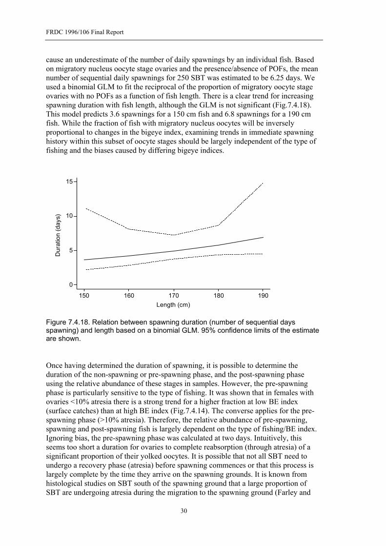
FRDC 1996/106 Final Report
cause an underestimate of the number of daily spawnings by an individual fish. Based on migratory nucleus oocyte stage ovaries and the presence/absence of POFs, the mean number of sequential daily spawnings for 250 SBT was estimated to be 6.25 days. We used a binomial GLM to fit the reciprocal of the proportion of migratory oocyte stage ovaries with no POFs as a function of fish length. There is a clear trend for increasing spawning duration with fish length, although the GLM is not significant (Fig.7.4.18). This model predicts 3.6 spawnings for a 150 cm fish and 6.8 spawnings for a 190 cm fish. While the fraction of fish with migratory nucleus oocytes will be inversely proportional to changes in the bigeye index, examining trends in immediate spawning history within this subset of oocyte stages should be largely independent of the type of fishing and the biases caused by differing bigeye indices.
150 160 170 180 190
0
5
10
15
Length (cm)
Dur
atio
n(d
ays)
Figure 7.4.18. Relation between spawning duration (number of sequential days spawning) and length based on a binomial GLM. 95% confidence limits of the estimate are shown. Once having determined the duration of spawning, it is possible to determine the duration of the non-spawning or pre-spawning phase, and the post-spawning phase using the relative abundance of these stages in samples. However, the pre-spawning phase is particularly sensitive to the type of fishing. It was shown that in females with ovaries <10% atresia there is a strong trend for a higher fraction at low BE index (surface catches) than at high BE index (Fig.7.4.14). The converse applies for the pre-spawning phase (>10% atresia). Therefore, the relative abundance of pre-spawning, spawning and post-spawning fish is largely dependent on the type of fishing/BE index. Ignoring bias, the pre-spawning phase was calculated at two days. Intuitively, this seems too short a duration for ovaries to complete reabsorption (through atresia) of a significant proportion of their yolked oocytes. It is possible that not all SBT need to undergo a recovery phase (atresia) before spawning commences or that this process is largely complete by the time they arrive on the spawning grounds. It is known from histological studies on SBT south of the spawning ground that a large proportion of SBT are undergoing atresia during the migration to the spawning ground (Farley and
30

FRDC 1996/106 Final Report
Davis 1998). As the majority of SBT are caught by shallow longlining methods (Davis and Farley 2001), which are associated with low BE indices, this would bias against the capture of pre-spawning fish that would normally remain at depth if not spawning. This would result in an underestimate of the duration of the pre-spawning phase. It is therefore likely that the pre-spawning phase is longer than two days and that, for many fish, this is completed by the time they reach the grounds or shortly after. In the absence of a satisfactory way of adjusting for the type of fishing or BE index, it is not possible to estimate the duration of the pre-spawning phase or to estimate what proportion of fish arriving on the ground are actually undergoing atresia. 7.5 Batch Fecundity Batch fecundity was determined on 37 SBT during both studies. Numbers were limited because of the specific criteria used in selecting ovaries for batch fecundity determinations and only 37 of 1115 ovaries were suitable. The relationship between fecundity and fish length was not a clear one, there being an increase in fecundity with length but with much variability (Fig. 7.5.1). Similarly, there was an increase in fecundity with increasing body weight and again this was highly variable (Fig. 7.5.2). This high variability has been observed for many tuna species – Euthynnus lineatus (Schaefer, 1987), Katsuwonus pelamis (Goldberg and Au, 1986), Thunnus albacares (Schaefer, 1998) and Thunnus obesus (Nikaido et al., 1991). This is possibly due to a large variation in batch size by individual fish depending on the stage of their spawning cycle. While there have been no direct observations of this in tunas, haddock are known to produce fewer eggs per successive spawnings when fed at maintenance rations (Hislop et al., 1978). There is also likely to be variation between spawning seasons as seen in anchovy (Hunter et al., 1985). We have insufficient data to examine seasonal and inter-annual differences on fecundity in SBT.
0
5
10
15
20
Batc
hfe
cund
ity(m
illion
s)
150 160 170 180 190 200Length (cm)
Figure 7.5.1. Batch fecundity of SBT by length. Fish age does not appear to provide additional information in regard to batch fecundity (Fig. 7.5.3) but this may be due to the extremely limited number of samples (8).
31
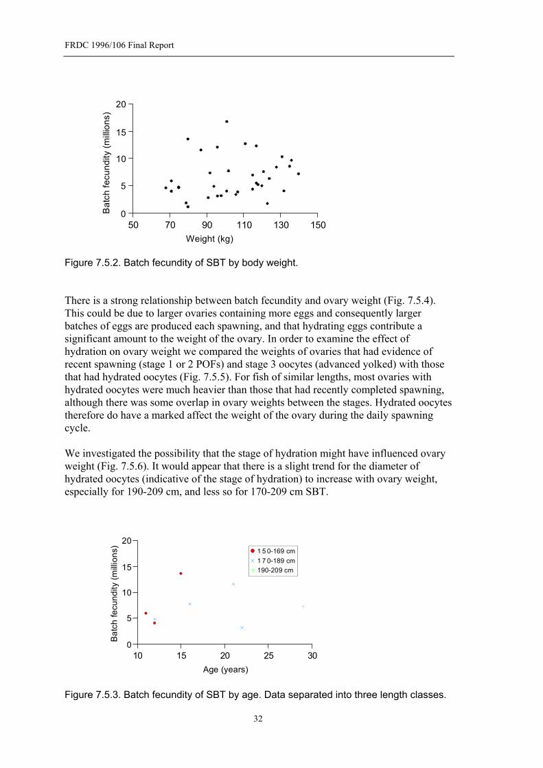
FRDC 1996/106 Final Report
50 70 90 110 130 1500
5
10
15
20B
atch
fecu
ndity
(milli
ons)
Weight (kg) Figure 7.5.2. Batch fecundity of SBT by body weight. There is a strong relationship between batch fecundity and ovary weight (Fig. 7.5.4). This could be due to larger ovaries containing more eggs and consequently larger batches of eggs are produced each spawning, and that hydrating eggs contribute a significant amount to the weight of the ovary. In order to examine the effect of hydration on ovary weight we compared the weights of ovaries that had evidence of recent spawning (stage 1 or 2 POFs) and stage 3 oocytes (advanced yolked) with those that had hydrated oocytes (Fig. 7.5.5). For fish of similar lengths, most ovaries with hydrated oocytes were much heavier than those that had recently completed spawning, although there was some overlap in ovary weights between the stages. Hydrated oocytes therefore do have a marked affect the weight of the ovary during the daily spawning cycle. We investigated the possibility that the stage of hydration might have influenced ovary weight (Fig. 7.5.6). It would appear that there is a slight trend for the diameter of hydrated oocytes (indicative of the stage of hydration) to increase with ovary weight, especially for 190-209 cm, and less so for 170-209 cm SBT.
10 15 20 25 30
190-209 cm1 7 0-189 cm1 5 0-169 cm
0
5
10
15
20
Batc
hfe
cund
ity(m
illion
s)
Age (years)
Figure 7.5.3. Batch fecundity of SBT by age. Data separated into three length classes.
32

FRDC 1996/106 Final Report
0 2000 4000 6000 8000 10000
190-209 cm1 7 0-189 cm1 5 0-169 cm
0
5
10
15
20
Batc
hfe
cund
ity(m
illion
s)
Ovary weight (g)
Figure 7.5.4. Batch fecundity by ovary weight. Data separated into three length classes.
150 160 170 180 190 200Length (cm)
0
2000
4000
6000
8000
10000
12000HydratedAdvanced yolk and stage 1 POFs
Advanced yolk and stage 2 POFs
Ova
ryw
eigh
t(g)
Figure 7.5.5. Ovary weight by fish length. Data grouped by hydrated oocyte stage (pe-spawning) and advanced yolk with early POFs (immediately after spawning) to examine the effects of hydration on ovary weight.
0200400600800
100012001400
0 2 4 6 8 10Ovary weight (kg)
Ooc
yte
diam
eter
(um
)
190-209 cm1 7 0-189 cm1 5 0-169 cm
12
Figure 7.5.6. Diameter of hydrated oocytes by ovary weight. Effect of stage of hydration on weight of ovary. Data grouped by 20 cm length class.
33
FRDC 1996/106 Final Report
7.6 Conclusions on Spawning and Effects of Depth of Fishing The present study has provided some new information on spawning dynamics in SBT, but its main value is that it has enabled refinement of previous estimates of spawning parameters and facilitated investigation of size/age and fisheries related trends in these parameters due to the greatly increased number of samples that were examined. The results of investigations on the depth of longline fishing using temperature-depth recorders generally confirmed that bigeye tuna tended to be caught at deeper hook positions than yellowfin tuna. An index based on the proportion of bigeye tuna in longline catches (BE Index) provides an indication of the depth of capture, however because of the imprecision inherent in the relationship between longline fishing depth (and how it is estimated) and catch, it can only be used to look for trends in data. Despite its looseness as a proxy for depth, the BE Index indicated how markedly the depth of fishing can affect estimation of parameters defining spawning dynamics. These effects will be raised where appropriate in drawing conclusions on the spawning parameters considered below. The spawning season was well defined previously, recent data only confirming what was already known. The spawning season starts in September and continues to April. There are generally two peaks in abundance of SBT on the spawning ground, one in October and one in January. The size of these peaks varies from year to year. The timing of spawning is influenced by the size and age of SBT. The smaller/younger ones are more abundant in the first half of the spawning season, with the middle sizes/ages more evenly spread throughout the spawning season, and the large/older fish more abundant in the second half of the spawning season. This trend seems to be reversed in the largest (200-219 cm) and oldest (28-32 year) group of SBT, but this could be because of the low number of fish in this group. As there is scope for bias in the size of fish caught due to depth of fishing, the relative size of each spawning peak might be affected by targeting in the fishery (as seen through the BE Index), as well as affected by changes in the size of recruitment of young spawners to the fishery on the spawning ground, and changes in the relative abundance of the larger/older SBT. SBT arriving on the spawning ground usually require a period of recovery before spawning commences. Farley and Davis (1998) found that SBT south of and in transit to the spawning grounds have a high incidence of atresia. SBT arrive on the spawning ground in this condition or just recovering from it. This is supported by the present study where the proportion of non-spawning fish and fish with >10% atresia is highest at the start of the spawning season, it then it drops to a fairly constant level. This is consistent with the first fish arriving at the beginning of the season all being in this pre-spawning recovering condition. From this point on there is a constant fraction of fish newly arriving that are recovering and those fish that have finished recovering and have entered the spawning phase. We consider that SBT undergo atresia to recover energy expended during migration that will be needed for spawning. This involves reabsorbing yolk (the process of atresia) and possibly rationalizing the supply of yolked eggs and reorganisation of the ovary before the start of spawning.
34
FRDC 1996/106 Final Report
SBT having <10% atresia are considered to have completed the pre-spawning phase and are ready to spawn, i.e. are in prime spawning condition (Farley and Davis 1998). Within this group of fish, the reciprocal of the proportion of spawning fish (those having post-ovulatory follicles indicative of spawning within previous 24 hours) provides an estimate of spawning interval. The weighted mean spawning fraction was 0.948 providing a spawning interval of 1.05 days (95% CL of mean, 1.04-1.07 days). Not all fish that are spawning are in prime spawning condition (~5%), although most are. As the condition is based on an arbitrary cut-off at <10% atresia, it is possible that some fish close to this state have started spawning. We found that the fraction of fish in prime spawning condition (having ovaries <10% atresia) and the fraction of spawning fish differed with fish length. The smallest size group (146-155 cm length class) having the lowest levels and the next size group the highest followed by a slight decline with size. Clearly the smallest size group is behaving differently to the larger fish, possibly because these parameters are being affected by the first maturation of part of this size class. There is little trend in spawning fraction with length when data are restricted to fish in prime spawning condition, i.e. they have completed the pre-spawning recovery phase or a possible resting phase between spawnings. This indicates the close link between being in prime spawning condition and spawning. If >10% atresia is associated with the post-migratory recovery phase only, it would suggest that no particular size group is more likely to have a resting period between daily spawning episodes once they are in prime spawning condition. If >10% atresia also occurs during rests between spawning episodes it then means that the relative duration of resting and prime spawning condition changes only slightly with fish size. Analysis of the effect of age on atresia and spawning fraction is limited by the reduced number of histological samples that had matching age determinations. Age showed similar trends to that of fish length but did not appear to provide any useful information that was not already provided by length. The BE Index as a proxy for depth has profound effects on a number of parameters measured in the course of this study and in the general catch monitoring of SBT on the spawning ground. This was first detected as affecting the observed length distributions of SBT caught by various sectors of the fishery (Davis and Farley, 2001). They found that small SBT are more likely to be caught at high levels of the BE index (in deep sets) than at low levels of the BE index (in shallow sets). It was interpreted that the size differentiation by depth was due to spawning activity, which was restricted to surface waters. The inference was that large fish spawn for longer than small fish and are subsequently exposed to surface fishing for longer than small fish and are hence more likely to be caught in shallow longline sets. Prior to this study there was insufficient histological samples to examine the relation between size and the proportion of spawning fish or spawning frequencies. Both the fraction of females in prime spawning condition and the fraction spawning is much higher at a low BE index (surface catches) than at a high BE index. The greatest difference occurs at the lowest BE Index where significantly higher fractions of SBT are in prime spawning condition and are spawning. It is this lowest BE Index that provides the “cleanest” proxy for depth as it will not be subject to problems of
35

FRDC 1996/106 Final Report
contamination by fishing at other depths. Some of the deeper hooks may catch fish before they settle or as they are being retrieved. The fraction of each size group of SBT that are caught at the surface increases with fish size. This means that larger SBT are exposed to surface fishing for longer than smaller fish. This suggests that the number of spawnings and/or the amount of time spent spawning or in courtship at the surface probably increases with fish size. We observed a trend for an increase in the number of consecutive daily spawnings with fish size, with 150 cm fish spawning on about 3.6 consecutive days and 190 cm fish spawning on about 6.8 consecutive days. The resting phase (>10% atresia) must also increase correspondingly with fish size, otherwise you would see an increase in the fraction of fish in prime spawning condition with size – which does not happen. This spawning duration is the number of consecutive daily spawnings that an individual fish makes. It is also possible that larger fish might have more than one spawning episode and rest between spawning episodes. We do not have any information on how long SBT remain on the spawning grounds. This type of information is best obtained by the use of archival tagging, and so far no archival tags have been recovered from SBT that have visited the spawning grounds. However, in a related species, Atlantic bluefin tuna (Thunnus thynnus), a 207 cm fish was recorded as moving into the Gulf of Mexico where it remained for 14 days undergoing behaviour suggestive of spawning (Block et al., 2001). This is what we would expect SBT to do, staying on the spawning grounds for only as long as necessary to complete spawning and then leaving. The relatively short duration on the ground for the Atlantic bluefin tuna would suggest a possible preliminary resting phase and then one series of consecutive daily spawnings, assuming that the number of consecutive daily spawnings was similar to that of the largest SBT in this study. Batch fecundity was also found to increase with fish size, although it was subject to great variability. Hunter et al. (1985) considered that at least 50 females were required to obtain an estimate of batch fecundity for northern anchovy to determine egg production. Considering the high variability found in this study it would appear that a greatly larger number of fecundity estimates are required. As this is exceedingly difficult to accomplish in any field program because of the very restrictive criteria used in the selection of ovaries, it would be very useful to identify a proxy for batch fecundity that does not have such a restricted sample size. One such measure might be the difference in ovary weight between fish with hydrated ovaries prior to spawning and fish with ovaries that have just spawned (i.e. have new POFs and no remaining hydrated oocytes) such as presented in Figure 7.5.5. This greatly increases the number of observations on which to estimate the change in batch fecundity with size. This approach is developed in the following section on population egg production.
36

FRDC 1996/106 Final Report
8. Population Egg Production In this section we estimate relative spawning contribution as a function of fish size. Spawning stock biomass (SSB) is widely recognized to be an imperfect proxy for total egg production of a population, and can yield misleading results when used as the “stock” axis in a stock-recruit relationship. Typically, SSB overstates the contribution of small fish, so that stock-recruit curves can show apparent hysteresis; the proportion of small fish is usually lower as a stock declines (at a given total SSB) than as the stock recovers, so recruitments in the recovery phase tend to be smaller than predicted using decline phase data. The way to avoid this is to use estimates of total egg production in place of SSB. Total egg production can be estimated by taking a weighted sum of assessed numbers-at-length, the weights being relative average individual egg production of different length classes. Neglecting the possibility of differential viability according to parental size, relative spawning contribution is proportional to expected per-capita egg production over a spawning season. In principle, this is simple to calculate for a mature fish: individualegg production of mature fish =(number of spawningevents)×(eggs per spawning) Eggs per spawning is also relatively easy to estimate, from histological data on ovary weights. However, the number of spawning events is harder to get at. One possible route is via: number of spawningevents=(duration onspawning ground)÷(averagespawning interval) Average spawning interval can be estimated from histological data. However, there is no obvious way of estimating duration on spawning ground; direct estimation will probably be impossible until the advent of archival tag data that covers spawning seasons, and for large (i.e. old) fish this will be some years in coming. There is one possible indirect route, relying on the fact that fish are fat when they arrive at the spawning grounds, but thin when they leave (Warashina and Hisada, 1970). By noting the date of first arrival of (say) 160cm fish, and the date at which thin 160cm fish are first found, it might be possible to form some estimate of the duration. A moment’s reflection, though, will indicate that this approach is fraught with difficulties. There is an additional difficulty. Note that: averageegg production of anyfish =(individualegg production)×(proportion mature) So that the proportion mature also needs to be estimated. It is clearly impossible to do this from data collected on the spawning ground, since all the fish on the spawning grounds are mature. Unfortunately, there are also major and probably insuperable difficulties associated with collecting appropriate off-spawning-ground data on pre- and non-spawners because of the protracted start to the spawning season and the asynchrony of spawning cycles of individual fish (Farley and Davis, 1998). A direct estimate of proportion-mature would require histological samples prior to the start of the spawning season, and away from the spawning ground. No such data are available.
37

FRDC 1996/106 Final Report
To circumvent all these difficulties, we have adopted a quite different approach. Consider the aggregate contribution of all fish of given length: total egg production=(total number of spawningevents)×(eggs per spawning) average individualegg production =(totalegg production)÷(number of fish) Again, eggs per spawning can be estimated from biological data. Estimated number of fish is available from the stock assessment, so the only missing quantity is total number of spawning events. In fact, since we are only interested in relative spawning contributions as a function of fish length, it is enough to estimate relative number of total spawning events across length classes. This is clearly going to be based somehow on the number of about-to-spawn fish in the samples. The calculation is not straightforward, though, because (i) the depth distribution varies with length and spawning status, and (ii) fishing mortality is distributed in an unknown and probably uneven pattern across depths. To deal with this, note that total number of spawning events for fish in a given length class can be calculated (in principle) via: total number of spawningevents
(total"fishdays"at that depth) spawning rateat that= ×∑ ( )depthsdepth
where spawning rate is implicitly in units of "events per day per fish while on the spawning grounds". Precise depth data are unavailable, but we can use the bigeye index (the ratio of bigeye catch to yellowfin catch), known to increase with setting depth as a proxy. The aim of the exercise is really to correct as far as possible for an observable relationship (the observed effect of bigeye index on spawning rate) which would bias results if ignored; once this is corrected for, we assume there is no residual effect of "true depth" requiring correction. Since we are only interested in relative average spawning contributions, both multiplicands can be considered in relative rather than absolute terms, i.e. compared to fish of some arbitrary reference length. Relative spawning rate at depth and length can be estimated from histological data. Total fishdays at depth and length and year is proportional to number of fish sampled at depth and length and year; under a few additional assumptions, it is possible to estimate statistically the relative per capita fishdays at depth for fish of different lengths (see below). The actual steps involved in producing a time series of total egg production, are as follows:
1. Use the histology data to estimate (relative) proportion that will spawn every day, by depth and length class.
2. Use (i) the length-depth data, (ii) a stock assessment, and (iii) some assumptions about sampling probability by depth, to establish (relative) average time spent by an individual fish on the spawning grounds, by depth and length.
3. Combine the two to predict RAISE (Relative Average Individual Spawning Events), by length.
4. Use the histology data to estimate relative batch fecundity, by length.
38
FRDC 1996/106 Final Report
5. Multiply RAISE by relative batch fecundity to get REPC (Relative Eggs Per Capita), by length.
6. To generate a time series of total (relative) egg production, take a time series of total numbers-at-length from a stock assessment (the same as in step 2), multiply by REPC, and sum across length classes within each year.
There are a couple of general points to note:
• This approach does not and cannot separate between a proportion mature and time spent on grounds; the same number of daily spawnings could arise from a group of fish with high proportion mature and low residence time, or vice versa. This does not matter whatsoever from the viewpoint of total egg production, but is important to bear in mind when comparing results to other approaches.
• Because the results rely on a specific assessment, which itself uses (part of) the same data, there is some apparent risk of circularity. However, the assessment does not explicitly use depth data, while the whole focus of the next few stages is on dealing with depth-related issues. The results are consistent with, but not an inexorable consequence of, whichever assessment is chosen. Closer linking with assessment is desirable, through incorporation of depth modelling into the assessment itself; doing this carefully will eliminate any risk of circularity.
• There is an implicit assumption that, for all fish that happen to be on the spawning grounds and within the same depth band at a given time, vulnerability to fishing gear in that depth band is equal. This seems reasonable; all the fish are large active predators within a fairly narrow size band (160-200cm). Note that this assumption is much weaker than assuming “catchability is constant” or “catchability at depth is constant”; there is an allowance for different vulnerabilities at depth, different depth distributions depending on size, and different lengths of stay on the spawning grounds depending on size.
8.1 Estimating Spawning Rates by Depth
Very few fish (about 2%) are caught during the daily act of spawning itself, i.e. with stage 1 POFs. In any case, because there is no guarantee that each spawning event lasts for the same amount of time regardless of length class, it would be dangerous to base estimates on direct counts of spawning fish. The histological data provides a better measure: presence of oocytes with migratory nuclei. Once nuclei have migrated, the progression to a spawning event within the next 12 or so hours (at any rate, less than 24 hours) is inevitable. Assuming that the time taken for eggs to develop from migratory nucleus stage to actual spawning is independent of fish length — a reasonable assumption, since this is simply a function of metabolism — then the proportion of fish (at given size and given depth) with migratory nuclei is an indicator of the relative spawning rate at that size and depth. An equivalent approach is to use the presence of POFs as a post hoc indicator of whether a fish has spawned within the last 24 hours. The two approaches give very similar answers, although the proportion with POFs is about 2.5X higher than the proportion with stage 4 or stage 5 oocytes. This simply indicates that the time taken to pass from the migratory nucleus stage to spawning is correspondingly less than the time taken for POFs to be reabsorbed.
39
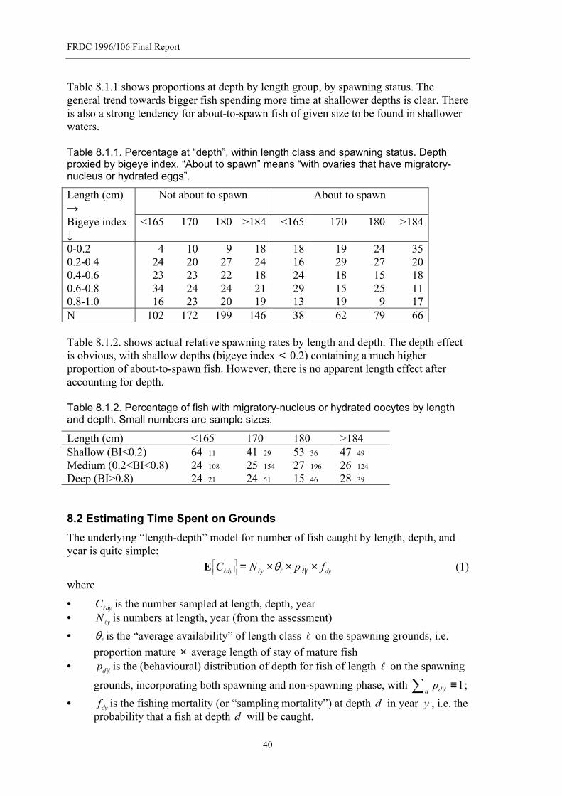
FRDC 1996/106 Final Report
Table 8.1.1 shows proportions at depth by length group, by spawning status. The general trend towards bigger fish spending more time at shallower depths is clear. There is also a strong tendency for about-to-spawn fish of given size to be found in shallower waters. Table 8.1.1. Percentage at “depth”, within length class and spawning status. Depth proxied by bigeye index. “About to spawn” means “with ovaries that have migratory-nucleus or hydrated eggs”.
Length (cm) →
Not about to spawn About to spawn
Bigeye index ↓
<165 170 180 >184 <165 170 180 >184
0-0.2 4 10 9 18 18 19 24 35 0.2-0.4 24 20 27 24 16 29 27 20 0.4-0.6 23 23 22 18 24 18 15 18 0.6-0.8 34 24 24 21 29 15 25 11 0.8-1.0 16 23 20 19 13 19 9 17 N 102 172 199 146 38 62 79 66 Table 8.1.2. shows actual relative spawning rates by length and depth. The depth effect is obvious, with shallow depths (bigeye index 0.2) containing a much higher proportion of about-to-spawn fish. However, there is no apparent length effect after accounting for depth.
<
Table 8.1.2. Percentage of fish with migratory-nucleus or hydrated oocytes by length and depth. Small numbers are sample sizes.
Length (cm) <165 170 180 >184 Shallow (BI<0.2) 64 11 41 29 53 36 47 49 Medium (0.2<BI<0.8) 24 108 25 154 27 196 26 124 Deep (BI>0.8) 24 21 24 51 15 46 28 39 8.2 Estimating Time Spent on Grounds
The underlying “length-depth” model for number of fish caught by length, depth, and year is quite simple: (1) dy y d dyC N pθ
| = × × ×E l l l l f
where
• is the number sampled at length, depth, year ldyCN• is numbers at length, year (from the assessment) ly
• is the “average availability” of length class on the spawning grounds, i.e. proportion mature × average length of stay of mature fish lθ l
• |ldp is the (behavioural) distribution of depth for fish of length l on the spawning
grounds, incorporating both spawning and non-spawning phase, with ; 1| ≡∑ lddp
• dyf is the fishing mortality (or “sampling mortality”) at depth in year , i.e. the probability that a fish at depth will be caught.
d yd
40
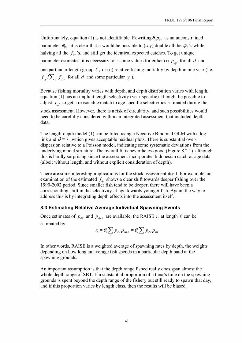
FRDC 1996/106 Final Report
Unfortunately, equation (1) is not identifiable. Rewriting |l d lpθ as an unconstrained parameter dφ ,l it is clear that it would be possible to (say) double all the 1φ l ’s while halving all the 1yf ’s, and still get the identical expected catches. To get unique parameter estimates, it is necessary to assume values for either (i)
dp ′|l
for all and
one particular length group or (ii) relative fishing mortality by depth in one year (i.e.
d′ ,l
dy d d yf f′ ′/∑ ′ ′ for all d and some particular ). y ′
Because fishing mortality varies with depth, and depth distribution varies with length, equation (1) has an implicit length selectivity (year-specific). It might be possible to adjust
dyf ′ to get a reasonable match to age-specific selectivities estimated during the
stock assessment. However, there is a risk of circularity, and such possibilities would need to be carefully considered within an integrated assessment that included depth data. The length-depth model (1) can be fitted using a Negative Binomial GLM with a log-link and which gives acceptable residual plots. There is substantial over-dispersion relative to a Poisson model, indicating some systematic deviations from the underlying model structure. The overall fit is nevertheless good (Figure 8.2.1), although this is hardly surprising since the assessment incorporates Indonesian catch-at-age data (albeit without length, and without explicit consideration of depth).
7θ = ,
There are some interesting implications for the stock assessment itself. For example, an examination of the estimated dyf shows a clear shift towards deeper fishing over the 1990-2002 period. Since smaller fish tend to be deeper, there will have been a corresponding shift in the selectivity-at-age towards younger fish. Again, the way to address this is by integrating depth effects into the assessment itself. 8.3 Estimating Relative Average Individual Spawning Events
Once estimates of dp |l and s dp | ,l are available, the RAISE at length can be estimated by
rl l
d s d d s dd d
r p p pθ θ p| | , | |= =∑ ∑l l l l l l
In other words, RAISE is a weighted average of spawning rates by depth, the weights depending on how long an average fish spends in a particular depth band at the spawning grounds. An important assumption is that the depth range fished really does span almost the whole depth range of SBT. If a substantial proportion of a tuna’s time on the spawning grounds is spent beyond the depth range of the fishery but still ready to spawn that day, and if this proportion varies by length class, then the results will be biased.
41

FRDC 1996/106 Final Report
0 5 10 15 20 25
05
1015
2025
Catch model: assess=OM 9RR5
fitted
obse
rved
Figure 8.2.1. Overall fit of the length-depth model. 8.3.1 Confidence Intervals and Effect of Assessment Choice on RAISE
Choice of assessment affects estimates of RAISE. The main reason for this is that if different assessments imply different length distributions, then the length-depth model has to adjust RAISE in order to predict the same number of about-to-spawn fish (which is the data being fitted to). Tables 8.3.1 and 8.3.2 show point estimates for different assessments (with f -at-depth assumed equal across depths; see below), together with 95% confidence intervals obtained by bootstrapping. The assessments used are the most “optimistic” and “pessimistic” assessments in Kolody and Polacheck (2001), known as OM9RR5 and PM2RR8 respectively. The uncertainty arising from s dp | is negligible compared to that arising from dp | .l
42
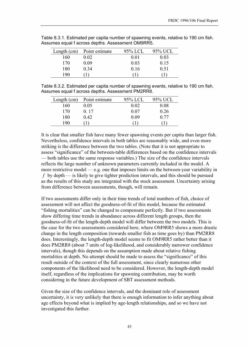
FRDC 1996/106 Final Report
Table 8.3.1. Estimated per capita number of spawning events, relative to 190 cm fish. Assumes equal f across depths. Assessment OM9RR5.
Length (cm) Point estimate 95% LCL 95% UCL 160 0.02 0.01 0.03 170 0.09 0.03 0.15 180 0.34 0.16 0.51 190 (1) (1) (1)
Table 8.3.2. Estimated per capita number of spawning events, relative to 190 cm fish. Assumes equal f across depths. Assessment PM2RR8.
Length (cm) Point estimate 95% LCL 95% UCL 160 0.05 0.02 0.08 170 0. 17 0.07 0.26 180 0.42 0.09 0.77 190 (1) (1) (1)
It is clear that smaller fish have many fewer spawning events per capita than larger fish. Nevertheless, confidence intervals in both tables are reasonably wide, and even more striking is the difference between the two tables. (Note that it is not appropriate to assess “significance” of the between-table differences based on the confidence intervals — both tables use the same response variables.) The size of the confidence intervals reflects the large number of unknown parameters currently included in the model. A more restrictive model — e.g. one that imposes limits on the between-year variability in f by depth — is likely to give tighter prediction intervals, and this should be pursued
as the results of this study are integrated with the stock assessment. Uncertainty arising from difference between assessments, though, will remain. If two assessments differ only in their time trends of total numbers of fish, choice of assessment will not affect the goodness-of-fit of this model, because the estimated “fishing mortalities” can be changed to compensate perfectly. But if two assessments show differing time trends in abundance across different length groups, then the goodness-of-fit of the length-depth model will differ between the two models. This is the case for the two assessments considered here, where OM9RR5 shows a more drastic change in the length composition (towards smaller fish as time goes by) than PM2RR8 does. Interestingly, the length-depth model seems to fit OM9RR5 rather better than it does PM2RR8 (about 7 units of log-likelihood, and considerably narrower confidence intervals), though this depends on the assumption made about relative fishing mortalities at depth. No attempt should be made to assess the “significance” of this result outside of the context of the full assessment, since clearly numerous other components of the likelihood need to be considered. However, the length-depth model itself, regardless of the implications for spawning contribution, may be worth considering in the future development of SBT assessment methods. Given the size of the confidence intervals, and the dominant role of assessment uncertainty, it is very unlikely that there is enough information to infer anything about age effects beyond what is implied by age-length relationships, and so we have not investigated this further.
43
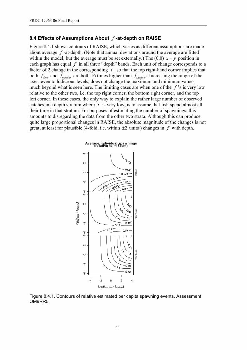
FRDC 1996/106 Final Report
8.4 Effects of Assumptions About f -at-depth on RAISE
Figure 8.4.1 shows contours of RAISE, which varies as different assumptions are made about average f -at-depth. (Note that annual deviations around the average are fitted within the model, but the average must be set externally.) The (0,0) x y− position in each graph has equal f in all three “depth” bands. Each unit of change corresponds to a factor of 2 change in the corresponding f , so that the top right-hand corner implies that both deepf and are both 16 times higher than mediumf shallowf . Increasing the range of the axes, even to ludicrous levels, does not change the maximum and minimum values much beyond what is seen here. The limiting cases are when one of the f ’s is very low relative to the other two, i.e. the top right corner, the bottom right corner, and the top left corner. In these cases, the only way to explain the rather large number of observed catches in a depth stratum where f is very low, is to assume that fish spend almost all their time in that stratum. For purposes of estimating the number of spawnings, this amounts to disregarding the data from the other two strata. Although this can produce quite large proportional changes in RAISE, the absolute magnitude of the changes is not great, at least for plausible (4-fold, i.e. within ± units ) changes in 2 f with depth.
-4-2
02
4
<165
cm
-4-2
02
4
165-
174c
m
-4-2
02
4
175-
184c
m
-4 -2 0 2 4
Average individual spawnings(relative to >185cm)
log2(fmedium÷ fshallow)
log 2
(f dee
p÷
f sha
llow)
Figure 8.4.1. Contours of relative estimated per capita spawning events. Assessment OM9RR5.
44

FRDC 1996/106 Final Report
8.5 Batch Fecundity
)
Batch fecundity was only determined for a small number of fish (37) between 1996 and 2002, and the very wide scatter makes it impossible to estimate the relationship with fish length to any precision; the point estimate of the slope of on
is 3.90 but with a standard error of 1.37. In this study, we have instead estimated batch fecundity indirectly, by the difference between ovary weights before and after spawning (for each size of fish) based on the data plotted in Figure 8.5.1. The working definitions of “before” and “after” are:
( )log fecundity(log length
• Before spawning: hydrated oocytes (stage 5) and no new POFs (to ensure that no partial spawning has occurred).
• After spawning: oocytes advance-yolked (stage 3), and with POFs. The point estimates of slopes on log-length are very similar (about 2.45 before spawning, vs. 2.51 afterwards), although the confidence interval on before-spawners is wide because there are only 51 such fish. On this evidence and a priori grounds, it is reasonable (but not proven) to assume that ovary weight increases by a constant proportion just before spawning, independent of fish length. There is a suggestion that variances are slightly higher for “before” fish (estimated residual standard error of 0.41 vs. 0.31), but allowing for this would make only a minor effect on point estimates and we have ignored it. We fitted a Gamma GLM with log-link to all the “before and after” fish, where intercept depends on before/after status but slope does not, i.e.:
(2) B
A
log E w log
log E w log
= β+ γ
= α + γl
l
l
l
for ovary weight w at length l , before/after indicated by B A/ , and parameters α, β and γ to be estimated (Figure 8.5.1). With this formulation, the relative batch fecundity of length compared to length is given by 2l 1l
1 1
2 2
1
2
− = −
l l
l l
l
l
B A
B A
w ww w
γ
(3)
which does not explicitly require estimates of β or α. The point estimate of γ is 2.47 (SE=0.21); since body weight is roughly proportional to
(actually 2.91 according to [Kolody and Polacheck, 2001]) and 2.47<3, this means that ovaries become lighter relative to body weight as (mature) fish continue to grow. Table 8.5.1 shows the corresponding relative batch fecundity across lengths, compared to a 190cm fish.
3l
45

FRDC 1996/106 Final Report
Table 8.5.1. Estimated batch fecundities, relative to a 190 cm fish1
Length (cm) Point estimate 95% LCL 95% UCL 160 0.66 0.61 0.70 170 0.76 0.73 0.80 180 0.88 0.86 0.89 190 1.00 1.00 1.00
4 .9 5 5 .00 5 .0 5 5.10 5 .15 5 .20 5 .25 5.3 06 .5
7 .0
7 .5
8 .0
8 .5
9 .0
9 .5
Log(fish length)
Log(
ovar
yw
eigh
t)
About to spawnJust spawned
5 .3 5
Figure 8.5.1. Ovary weight versus fish length. Small dots/thin line are ovaries at stage 3 (advanced yolked oocytes) with stage 1 and 2 POFs and solid/thick line are ovaries at stage 5 (hydrated oocytes) and without stage 1 POFs. Regression lines have different intercepts but identical slopes. The point estimate of β α− is 0.28 (SE=0.05), indicating that about 33% of the hydrated ovary weight is lost during each spawning event. Although the confidence interval is fairly tight, this depends on an assumption (supported, but not proved by, the data) that the slopes of the regressions in Figure 8.5.1 really are equal, i.e. that hydration increases the weight of an ovary by a constant proportion (33%), regardless of fish length. More support for this plausible assumption could be obtained either by getting more samples from hydrated-oocyte fish, or by looking at data for other tunas. It is interesting to note that heavier fish have proportionally lighter gonads relative to body weight. This is based on a large sample size, and cannot be due to sampling noise. 1 Strictly speaking, the table applies only to fish of the exact size indicated. In practice, the actual mean lengths within each length class (155-165, 165-174, 175-184, 185+ cm) are very close to the sizes given. However, because the length-to-weight-loss relationship is nonlinear, the mean length within a length class won’t correspond to the mean ovary weight loss. Nevertheless, the results will not be much affected by this— certainly less than the spread of standard errors.)
46

FRDC 1996/106 Final Report
The point estimate based on direct batch fecundity measurements, however, would imply the opposite (i.e. proportionally heavier gonads relative to body weight). This is presumably an accident that reflects the very large variability associated with the direct measurements. 8.6 Forming a time series of relative egg production
Three choices have to be made to produce a time series of relative egg production:
• which assessment to use (i.e. which time series of numbers-at-length); • which relative f ’s at depth to use, in some reference year; • batch fecundity at length: which relationship to use?
Once these choices have been made, model (1) can be fitted and used to predict RAISE. Multiplying RAISE by relative batch fecundity gives a table of relative eggs per capita (REPC) by length. For the equal- f -at-depth model (Tables 8.3.1 and 8.3.2) and the point estimates of relative batch fecundity (Table 8.5.1), the point estimates of REPC under assessments OM9RR5 and PM2R88 are shown in Table 8.6.1. Table 8.6.1. Relative egg production per capita by length, combining RAISE and batch fecundity.
Length (cm) OM9RR5 PM2RR8 160 0.012 0.034 170 0.071 0.127 180 0.294 0.37 190 (1) (1)
To estimate egg production in a given year, the numbers in one column of this table then simply need to be multiplied by numbers-at-length from the corresponding assessment, and summed across the four length classes. Table 8.6.1 contains “egg production ogives” by length, which can be converted to an age ogive using length-at-age data (here taken from proportions in the recent assessment, and so applicable only to more recent cohorts). This can be compared with the age-specific SSB (i.e. average weight at age × ppn. mature at age) estimated in the asssessment itself (Figure 8.6.1; the picture for assessment PM2RR8 is similar). It must be emphasized that the conversion to age is very crude, because the 10cm length classes in the assessment are much too big to allow accurate back-conversions. Nevertheless, the general implication is clear; under the assumptions here, fish are not reaching 50% spawning potential until about age 17 years, compared with about age 11 years that is estimated if relative fecundity is ignored. The big difference between the two curves in Figure 8.6.1 can be explained by larger fish staying on the grounds for much longer than smaller fish. This is reflected by the relative over-abundance of large fish in the Indonesian catch data compared to the assessment, after adjusting for depth effects.
47
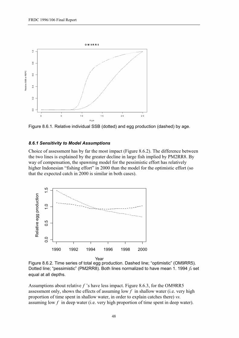
FRDC 1996/106 Final Report
0 5 1 0 1 5 2 0 2 5
0.0
0.2
0.4
0.6
0.8
1.0
O M 9 R R 5
A g e
Rel
ativ
e SS
B or
REP
C
Figure 8.6.1. Relative individual SSB (dotted) and egg production (dashed) by age. 8.6.1 Sensitivity to Model Assumptions
Choice of assessment has by far the most impact (Figure 8.6.2). The difference between the two lines is explained by the greater decline in large fish implied by PM2RR8. By way of compensation, the spawning model for the pessimistic effort has relatively higher Indonesian “fishing effort” in 2000 than the model for the optimistic effort (so that the expected catch in 2000 is similar in both cases). Figure 8.6.2. Time series of total egg production. Dashed line; “optimistic” (OM9RR5). Dotted line; “pessimistic” (PM2RR8). Both lines normalized to have mean 1. 1994 df set equal at all depths.
1990 1992 1994 1996 1998 2000
0.0
0.5
1.0
1.5
Year
Rel
ativ
e eg
g pr
oduc
tion
Assumptions about relative f ’s have less impact. Figure 8.6.3, for the OM9RR5 assessment only, shows the effects of assuming low f in shallow water (i.e. very high proportion of time spent in shallow water, in order to explain catches there) vs. assuming low f in deep water (i.e. very high proportion of time spent in deep water).
48

FRDC 1996/106 Final Report
These are extreme assumptions, but produce only about a 10% difference at most. Differences are even less for assessment PM2RR8. Figure 8.6.3. Total egg production relative to mean. Dashed line; low f on shallow. Dotted line; low f on deep. The relationship between batch fecundity and length is moderately well determined, but the exponent of the relationship is still subject to some uncertainty. In principle, bigger values for the exponent will increase the relative spawning contribution of bigger fish. However, as shown in Figure 8.6.4, the projected difference in relative egg production across this time period is imperceptible in practice. Taking a 190cm fish as the baseline, then changing from the upper to the lower 95% confidence limit of the exponent only produces about a 5% increase in the relative batch fecundity of a 180cm fish, rising to about a 15% increase for 160cm fish. Since smaller fish spawn much less often than larger fish, these changes are diluted even further when considering total egg production.
1990 1992 1994 1996 1998 2000
0.0
0.5
1.0
1.5
Year
Rel
ativ
e eg
g pr
oduc
tion
1990 1992 1994 1996 1998 2000
0.0
0.5
1.0
1.5
Year
Rel
ativ
e eg
g pr
oduc
tion
Figure 8.6.4. Total egg production relative to mean. Solid line uses point estimate of 2.47: dotted and dashed lines are lower and upper 95% confidence limits (~2.1 and ~2.0). Assessment OM9RR5, equal f across depths.
49
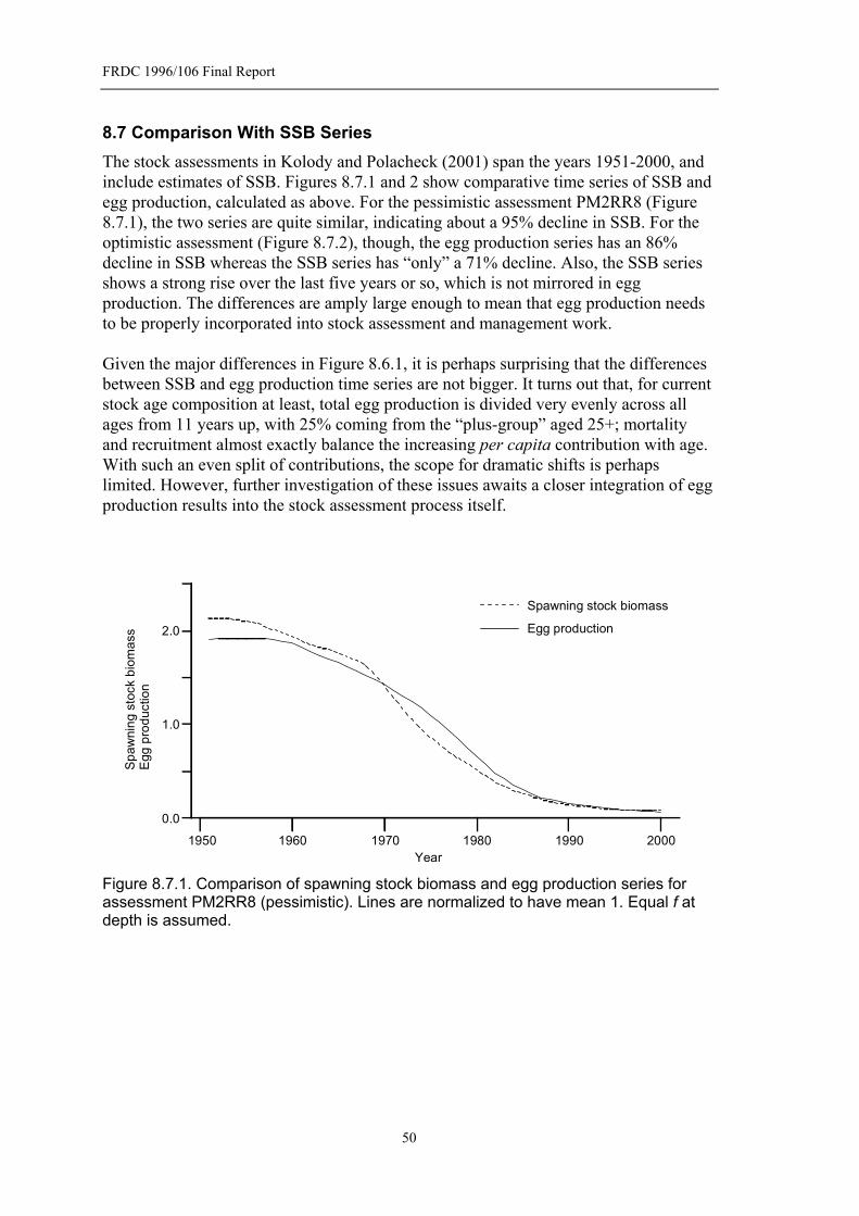
FRDC 1996/106 Final Report
8.7 Comparison With SSB Series
The stock assessments in Kolody and Polacheck (2001) span the years 1951-2000, and include estimates of SSB. Figures 8.7.1 and 2 show comparative time series of SSB and egg production, calculated as above. For the pessimistic assessment PM2RR8 (Figure 8.7.1), the two series are quite similar, indicating about a 95% decline in SSB. For the optimistic assessment (Figure 8.7.2), though, the egg production series has an 86% decline in SSB whereas the SSB series has “only” a 71% decline. Also, the SSB series shows a strong rise over the last five years or so, which is not mirrored in egg production. The differences are amply large enough to mean that egg production needs to be properly incorporated into stock assessment and management work. Given the major differences in Figure 8.6.1, it is perhaps surprising that the differences between SSB and egg production time series are not bigger. It turns out that, for current stock age composition at least, total egg production is divided very evenly across all ages from 11 years up, with 25% coming from the “plus-group” aged 25+; mortality and recruitment almost exactly balance the increasing per capita contribution with age. With such an even split of contributions, the scope for dramatic shifts is perhaps limited. However, further investigation of these issues awaits a closer integration of egg production results into the stock assessment process itself.
Egg production
Spawning stock biomass
1950 1960 1970 1980 1990 2000Year
0.0
1.0
2.0
Spaw
ning
stoc
kbi
omas
sEg
gpr
oduc
tion
Figure 8.7.1. Comparison of spawning stock biomass and egg production series for assessment PM2RR8 (pessimistic). Lines are normalized to have mean 1. Equal f at depth is assumed.
50

FRDC 1996/106 Final Report
s
as
biom
ock
gst
nin
paw
S Egg
prod
uctio
n
1950 1960 1970 1980 1990 2000Year
0.0
1.0
2.0 Egg production
Spawning stock biomass
Figure 8.7.2. Comparison of spawning stock biomass and egg production series for assessment OM9RR5 (optimistic). Lines are normalized to have mean 1. Equal f at depth is assumed. 9. Conclusions All objectives in this project were met, although some of these have not been presented explicitly as they were either an intermediate step in the population egg production model or had been replaced by a more relevant and improved parameter. The mean size at maturity of SBT on the spawning grounds (Objective 1) was not estimated explicitly as it was integrated in - the “average availability” of length class on the spawning grounds as in equation 1, Section 8.2. This term incorporates (i) the proportion mature at a particular length × (ii) the average duration of stay of mature fish of that length on the spawning ground. It provides the average relative duration a fish of a given length spends on the spawning ground. This term has the most profound effect on population egg production of all the parameters in the egg production model.
lθ l
Objective 2, the relationship between spawning frequency and size was determined from the histology data. Once fish start a spawning cycle on the spawning grounds they spawn daily, irrespective of size. However, they undergo a resting phase on arrival at the spawning grounds before starting spawning, and if they undergo more than one spawning cycle will rest between cycles. The relative proportion of time spent resting/recovering and time spent spawning also varied with size. This information was used in conjunction with information on the depth distribution by size to estimate the relative proportion of fish that would spawn every day by depth and length class. Both duration and depth integrated spawning frequency were then used to determine the relative average individual spawning events for a fish of a given size. The relationship between batch fecundity and size (Objective 3) was determined indirectly after it was found that direct fecundity estimates were (naturally) so highly variable that it would not be possible to ever obtain a sufficient number of estimates to give the precision required in an egg production model. Instead, we determined the relative batch fecundity based on the ovary weight difference between a fish about to
51

FRDC 1996/106 Final Report
spawn and one that had just completed the daily spawning event. Relative batch fecundity was consistent with the relationship between direct measurements of batch fecundity and size, however it could be estimated more precisely. The product of relative batch fecundity and relative average number of individual spawning events then provided relative egg production by size. The egg production model (Objective 4) uses numbers at length from a stock assessment to estimate the relative average duration a fish of a given length spends on the spawning ground (duration) and to generate a time series of total relative egg production. The choice of stock assessments will change the estimates of these parameters slightly. However, the difference in relative egg production with size are profound (see Table 9.1) regardless of which assessment of Kolody and Polacheck (2001) is used. There is a two orders of magnitude difference in the point estimates of relative egg production between a 160 cm and 190 cm fish for the most pessimistic assessment. This difference is only slightly less for the most optimistic assessment. This will have profound effects on the recovery of egg production by a population as 50% recruitment into population egg production is not reached until 17 years whereas 50% recruitment into the spawning stock biomass in reached at 11 years. These differences are amply large enough to warrant properly incorporating egg production into stock assessments. Table 9.1. Point estimates for parameters in the egg production model relative to a 190 cm fish. Duration includes proportion mature and average length of stay of mature fish of a given length on the spawning ground. RAISE is relative average individual spawning events for a fish of a given size determined from duration x their depth integrated spawning frequency. Egg production is RAISE x batch fecundity.
OM9RR5 - most optimistic assessment
Length (cm) Batch fecundity Duration RAISE Egg production
160 0.66 0.02 0.02 0.01
170 0.76 0.10 0.09 0.07
180 0.88 0.35 0.34 0.30
190 1.00 1.00 1.00 1.00
PM2RR8 - most pessimistic assessment
Length (cm) Batch fecundity Duration RAISE Egg production
160 0.66 0.06 0.05 0.03
170 0.76 0.18 0.17 0.13
180 0.88 0.44 0.42 0.37
190 1.00 1.00 1.00 1.00
52

FRDC 1996/106 Final Report
10. Benefits The development of a population egg production model provides a greatly improved indicator of spawning potential for use in stock assessment and prediction than the currently used spawning stock biomass. The differences are amply large enough to warrant properly incorporating egg production into stock assessments. The main benefits are likely to be in better stock predictions as the stock-recruitment relationship is genuinely based on spawning potential not just on biomass of the spawning stock. This will ultimately produce better management advice for managers of the SBT fishery. 11. Planned Outcomes This study has provided new information on the spawning dynamics of SBT and this has enabled us to refine previous estimates of spawning parameters and investigate size/age and fisheries related trends in these parameters. With this increased understanding of spawning dynamics we have been able to determine size related changes in the key parameters needed to develop an egg production model for SBT. We have successfully produced an egg production model that uses information on spawning derived from histology, information on the temporal distribution of SBT by depth on the spawning ground, and information on numbers at length from a stock assessment. The resulting population egg production provides a greatly improved indicator of spawning stock biomass for use in stock assessment and prediction. The main benefits are likely to be in better predictions. Using spawning stock biomass as a proxy for spawning potential gives quite a different stock-recruitment relationship during a period of stock decline, than during the subsequent recovery. However, this artifact disappears if a better proxy for spawning potential, such as population egg production is used. Stock projections to examine medium to long term consequences of current catches on parental biomass and the probability of recovery to the 1980 levels depend on good information on the recruitment dynamics of population egg production. We have provided this, and as expected, the two orders of magnitude difference in the relative egg production of a 160 cm and 190 cm fish will have profound effects on how long it takes for the SBT population to recover to 1980 levels of egg production. These differences are amply large enough to warrant properly incorporating egg production into stock assessments to provide better stock predictions and improved information for managers. We will work together with the stock assessment group at CSIRO Marine Research to ensure that egg production is integrated in a consistent way within the stock assessment framework. 12. Further Development 12.1 Further data requirements
12.1.1 Histology
There is now a large sample of histological data (941 fish), allowing a good understanding of the dynamics of spawning. For the purposes of estimating relative spawning potential by size, the histology data have successfully allowed identification soon-to-spawn fish (oocyte stages 4 and 5) and post-spawning-event fish (presence of
53

FRDC 1996/106 Final Report
post-ovulatory follicles). Although questions do remain about the biology of tuna spawning (resting periods, duration at spawning grounds, proportion mature), the existing data are largely sufficient for linking with assessment work. The main exception concerns the relationship between batch fecundity and size, which is somewhat uncertain. The impact on time series of egg production appears to be small in comparison to other sources of uncertainty. However, this somewhat rests on an assumption which, though a priori plausible and certainly consistent with available data, is not yet proven: that the weight of hydrated ovaries (i.e. immediately pre-spawning-event) scales with length in the same way as the weight of post-spawning-event ovaries. How could this situation be bettered? At the moment, the standard error of the exponent of on is about 1.4. To reduce this to a reasonable level of around 0.25, a 25-fold increase in the number of samples would be required! The situation is slightly better for estimates of hydrated ovary weights, which have been measured more often and show less individual variation, but even so about a 12-fold increase in sample size would be needed to get standard errors down to the same level. Direct evidence via sampling along existing lines therefore seems unattainable in the near future. As a cheap preliminary step, studies from other species might provide enough circumstantial evidence to lend credence to this assumption.
(log direct batch fecundity) (log length)
12.1.2 Biological Data on Depth Distribution
It is possible to fit the data equally well with different assumptions about average f -at-depth, by varying the estimated depth distribution (i.e. time-at-depth) in inverse proportion. Thus, there is no way to separate these two phenomena statistically, even though the depth distribution does affect the relative spawning contribution of different lengths. Although there are limits to the overall effect this can have on time series of egg production, there is still room for making a substantial improvement in precision if more data can be collected to pin down either relative f -at-depth (in any one year), or relative time at depth (in any one length group). The former seems intractable, but time-at-depth could be assessed accurately from archival tag data. Archival tag data would also allow direct estimation of duration on the spawning grounds. At a minimum, this would provide a useful consistency check on estimates of availability by age. More ambitiously, though, duration on grounds could be used to provide estimates of relative abundance by length that are effectively independent of the rest of the assessment. Assuming equal catchability for all sizes of fish present on the grounds at a particular depth, then the number of captures at that depth (relative across length classes) will be proportional to relative abundance of length classes, times the mean duration on the grounds. As well as helping to establish an unambiguous direct biological estimate of relative egg production, this would be of great value to the assessment itself.
54

FRDC 1996/106 Final Report
12.2 Further Integration with Assessment This report provides a template for incorporating improved “SSB” series in stock assessment and prediction. The main benefits are likely to be in better predictions. If a “stock-recruitment” relationship is genuinely based on spawning potential, it is more likely that the past will be a useful guide to the future. One example is North Sea herring (ICES, 1998), where using SSB as a proxy for spawning potential gives quite a different S-R relationship during a period of stock decline, than during the subsequent recovery (which was slower than expected). However, this artifact disappears if a better proxy for spawning potential is used. To actually incorporate these results into assessment, further work will be required in the stock assessment itself. The recalculation of spawning potential and fitting of stock-recruit relationships is comparatively easy, but there are two related issues to be addressed. 12.2.1 Reducing circularity
The approach used here should be seen as consistent with, rather than a circular by-product of, any chosen stock assessment. The focus is on reducing depth-sampling biases in the length data, and in incorporating depth effects on spawning frequency, while the assessment itself does not use depth data. However, there is another area where circularity potentially does arise. The stock assessments in Kolody and Polacheck (2001) have an internally-estimated stock-recruit relationship based on SSB, so the estimated stock sizes used here already incorporate some stock-recruit modeling. This is philosophically awkward. In practice, though, stock-recruit relationships are so ineffective at predicting individual cohort strengths (where CVs of 60% are typical) that very little predictive power is gained by including the stock-recruit relationship inside the assessment. This mitigates the risk of circularity. However, in further work, close attention should be paid to this point. 12.2.2 Including Length-Depth Modeling
The results of this analysis depend to some extent on length-depth modeling of fishery selectivity in Indonesia. There is also a signal in the data, in that some assessment series are easier to reconcile with the length-depth data than others. This suggests it might be worth considering whether a length-depth model of the form used here (even without the knock-on effects for stock and recruitment) might be incorporated into the assessment framework in its own right. Equally, some further consideration of plausible f -at-depth models from a stock assessment perspective could help in tightening up
confidence intervals on spawning potential. In all this, it will again be particularly important to take good care to avoid any danger of circularity.
55

FRDC 1996/106 Final Report
13. References Block, B.A., Dewar, H., Blackwell, S.B., Williams, T.D., Prince, E.D., Farwell, A.B.,
Teo, S.L.H., Seitz, A., Walli, A., and Fudge, D. 2001. Migratory movements, depth preferences, and thermal biology of Atlantic bluefin tuna. Sci. 293: 1310-1314.
Clear, N.P., Gunn, J.S., Rees, A.J. 2000. Direct validation of annual increments in the otoliths of juvenile southern bluefin tuna, Thunnus maccoyii, through a large-scale mark-and-recapture experiment using strontium chloride. Fish. Bull. 98, 25-40.
Davis, T.L.O. and Andamari. R. 2002. Catch Monitoring Of The Fresh Tuna Caught By The Bali-Based Longline Fishery in 2001. Report for the CCSBT Scientific Meeting, 9-11 September 2002, Canberra, Australia. CCSBT/SC/0209/01.
Davis , T.L.O., and Farley, J.H. 2001. Size partitioning by depth of southern bluefin tuna (Thunnus maccoyii) on the spawning ground. Fish. Bull. 99:381-386.
Farley, J.H. and Davis, T.L.O. 1998. Reproductive dynamics of southern bluefin tuna, Thunnus maccoyii. U.S. Fish. Bull. 96: 223-236.
Farley, J.H. and Davis, T.L.O. 2002. Length and age distribution of SBT in the Indonesian longline catch on the spawning ground. Report for the CCSBT Scientific Meeting, 9-11 September 2002, Canberra, Australia. CCSBT/SC/0209/02.
Fitzhugh, G. R., and W. F. Hettler. 1995. Temperature influence on postovulatory follicle degeneration in Atlantic menhaden, Brevoortia tryannus. Fish. Bull. 93:568-572.
Gunn, J.S., Clear, N.P., Carter, T.I., Rees, A.J., Stanley, C.A., Farley, J.H., Kalish, J.M., In Press. The direct estimation of age and growth in southern bluefin tuna, Thunnus maccoyii (Castelnau), using otoliths, scales and vertebrae. Fish. Bull.
Goldberg, S.R., and Au, D.W.K. 1986. The spawning of skipjack tuna from southeastern Brazil as determined from histological examinations of ovaries. In “Proceedings of the ICCAT Conference on the International Skipjack Year Program” (Symons, P.E.K., Miyake, P.M., and Sakagawa, G.T., Eds.), pp. 277-284, ICCAT, Madrid, Spain.
Hislop, J.R.G., Robb, A.P., and Gauld, J.A. 1978. Observations on the effects of feeding level on growth and reproduction in haddock, Melanogrammus aeglefinus (L.) in captivity. J. Fish Biol. 13: 85-98.
Hunter, J. R., and S. R. Goldberg. 1980. Spawning incidence and batch fecundity in northern anchovy, Engraulis mordax. Fish. Bull. 77:641-652.
Hunter, J. R., Lo, N.C.H., and Leong, R.J.H. 1985. Batch fecundity in multiple spawning fishes. U.S. Nat. Mar. Fish. Serv., Nat. Oceanic Atmos. Adm., Tech. Rep. 36: 79-94.
Hunter, J. R., and B. J. Macewicz. 1980. Sexual maturity, batch fecundity, spawning frequency, and temporal pattern of spawning for the northern anchovy, Engraulis mordax, during the 1979 spawning season. Calif. Coop. Oceanic Fish. Invest. Rep. 21:139-149.
Hunter, J. R., and B. J. Macewicz.1985a. Measurement of spawning frequency in multiple spawning fishes. In R. Lasker (ed.), An egg production method for estimating spawning biomass of pelagic fish: application to the northern anchovy, Engraulis mordax. U.S. Dep. Commer., NOAA Tech. Rep. NMFS 36:79-94.
56

FRDC 1996/106 Final Report
Hunter, J. R., and B. J. Macewicz. 1985b. Rates of atresia in the ovary of captive and wild northern anchovy, Engraulis mordax. Fish. Bull. 83:119-136.
Hunter, J. R., B. J. Macewicz, and J. R. Sibert. 1986. The spawning frequency of skipjack tuna, Katsuwonus pelamis, from the south Pacific. Fish. Bull. 84:895-903.
ICES, 1998. Report of the Study Group on Stock-Recruitment Relationships for North Sea Autumn-Spawning Herring. Lowestoft, UK 26-28 May 1998. International Counc. for the Exploration of the Sea. ICES-CM-1998/D:2.
Kolody, D. and T. Polacheck. 2001. Application of a statistical catch-at-age and -length integrated analysis model for the assessment of southern bluefin tuna stock dynamics 1951-2000. Report for the CCSBT Scientific Meeting, 28-31 August 2001, Tokyo, Japan. CCSBT-SC/0108/13.
Lowerre-Barbieri, S. K., and L. R. Barbieri. 1993. A new method of oocyte separation and preservation for fish reproduction studies. Fish. Bull. 91(1):165-170.
Nikaido, H., N. Miyabe, and S. Ueyanagi. 1991. Spawning time and frequency of bigeye tuna, Thunnus obesus. Bull. Nat. Res. Inst. Far Seas Fish. 28:47-73.
McPherson, G. R. 1988. Verification of the postovulatory follicle method for establishing the spawning frequency of yellowfin, bigeye and skipjack tuna in the Coral Sea. Qld. Dept. Prim. Ind., Fish. Res. Branch, Tech. Rep. FRB 88/9, 42pp.
McPherson, G. R. 1991. Reproductive biology of yellowfin tuna in the eastern Australian fishing zone, with special reference to the North-western Coral Sea. Aust. J. Mar. Freshwater Res. 42:465-477.
Nikaido, H., Miyabe, N., and Ueyanagi, S. 1991. Spawning time and frequency of bigeye tuna, Thunnus obesus. Nat. Res. Inst. Far Seas Fish., Bull. 28: 47-73.
Schaefer, K. M. 1996. Spawning time, frequency, and batch fecundity of yellowfin tuna, Thunnus albacares, near Clipperton Atoll in the eastern Pacific Ocean. Fish. Bull. 94:98-112.
Schaefer, K. M. 1987. Reproductive biology of black skipjack, Euthynnus lineatus, an eastern pacific tuna. Inter-Amer. Trop. Tuna Comm. Bull. 19:169-260.
Schaefer, K. M. 1998. Reproductive biology of yellowfin tuna (Thunnus albacares) in the eastern Pacific Ocean. Inter-Amer. Trop. Tuna Comm. Bull. 21: 201-272.
Suzuki, Z. and Nishida, T. 1997. Comparison of information on the catch and size of fish in the spawning ground of southern bluefin obtained from Indonesian and Japanese longline fisheries. Report for the CCSBT Scientific Meeting, 28 July-8 August 1997, Canberra, Australia. CCSBT/SC/97/13.
Warashina, I., and Hisada, K. 1970. Spawning activity and discoloration of meat and loss of weight in the southern bluefin tuna. Bull. Far Seas Fish. Res. Lab. 3: 147-167.
57

FRDC 1996/106 Final Report
14. Intellectual property No commercial intellectual property arose from this work 15. Staff Tim Davis1 Principal Investigator Jessica Farley1 Biologist Thor Carter1 Technician Mark Bravington2 Statistician/modeler Poppy Andamari3 Indonesian project leader 1CSIRO Marine Research, Hobart, Tasmania 2 CSIRO Mathematical and Information Sciences 3 Indonesian Research Institute of Marine Fisheries 16. List of appendices Appendix 1. Southern bluefin tuna: Quantifying reproductive status from histological sections, and estimating batch fecundity.
58
Appendix 1
Southern bluefin tuna:
Quantifying reproductive status from histological sections, and estimating batch
fecundity
Jessica Farley and Tim Davis
CONTENTS
Tasks ................................................................................................................................ 3 1 Ovary collection...................................................................................................... 3 2 Ovary subsampling ................................................................................................. 3 3 Histological analysis ............................................................................................... 3 4 Batch fecundity estimation ..................................................................................... 4
Oocyte descriptions......................................................................................................... 7 1 Unyolked stage ....................................................................................................... 7 2 Early yolked stage................................................................................................... 7 3 Advanced yolked stage ........................................................................................... 8 4 Migratory nucleus stage.......................................................................................... 8 5 Hydrated stage ........................................................................................................ 9
Postovulatory follicle (POF) descriptions ................................................................... 11
1 New POFs (0 hours old) ....................................................................................... 11 2 POFs < 12 hours old ............................................................................................. 11 3 POFs 12 - 24 hours old ......................................................................................... 12
Atretic oocyte descriptions........................................................................................... 13 1 Alpha atresia ......................................................................................................... 13 2 Beta atresia............................................................................................................ 13
Decaying ovary tissue ................................................................................................... 15
Data entry forms ........................................................................................................... 16
1 SBT ovary form .................................................................................................... 16 2 Reproduction form................................................................................................ 17
References...................................................................................................................... 18
2

TASKS
1 Ovary collection Southern bluefin tuna ovaries are to be collected in one of two ways, depending on where the fish is gutted. If gutted at sea, the ovaries will be removed by the captain, labelled, placed in a sample bag and put on ice. The tuna carcass will be given a matching label so that the fish and ovaries can be identified when the catch is landed. If the fish is not gutted at sea, the ovaries will be removed at the processing plant. Each ovary is to be labelled with sample number, vessel name and landing date matching these entries on the landings form. The fork length (to the nearest cm) and dressed weight (to the nearest kg) of each fish sampled is to be measured. Record the vessel name, date landed, sample number (ovary), fish length and weight etc on the landings forms. All ovaries should be held on ice until collected by the coordinator. Ovaries should be collected and processed by the coordinator as soon as possible.
2 Ovary subsampling
At the processing plant by the coordinator After removing excess fat, weigh each ovary to the nearest g. Remove a core sample of material from each ovary (using the coring instrument provided), weigh to the nearest 0.01 g and place in a glass vial with 10% buffered formalin. Inspect each ovary to determine if it is suitable for batch fecundity estimates. To do this, make a small incision in the ovary and remove some eggs. If hydrated eggs are present, the ovary is suitable for batch fecundity estimates. An egg is hydrated when it is large and round (approximately 1mm in diameter) and has a transparent appearance (see figure 2F in Farley and Davis [1998]). If hydrated eggs are present in the lumen of the ovary, it is not suitable for fecundity estimates, as the ovary has lost eggs. Label and freeze all ovaries suitable for fecundity estimates. Data to be recorded on the “SBT ovary form”. Example on p16. • Sample number • Vessel name • Landing date • Ovary weight • Ovary condition – suitable for batch fecundity?
3 Histological analysis
In the Gondol laboratory Remove the ovary sample from the vial and cut off a portion suitable for histological processing. From the remaining sample, measure the diameter of 10 of the most advanced eggs (oocytes) for each ovary to the nearest 0.1µm, under a stereomicroscope.
3

Prepare histological sections (stained with haemotoxylin and eosin) for each ovary sample, and examine under a compound microscope. Classify each section using the following criteria: 1. Oocyte stage:
Classify the most advance group of eggs in each ovary. Eggs will be either unyolked (1), early yolked (2), advanced yolked (3), migratory nucleus (4) or hyrdated (5). See oocyte descriptions and figures; and figures 2A to 2C in Farley and Davis (1998).
2. Postovulatory follicle stage (POF): Classify POFs as either absent (0), new (1), less than 12 hours old (2), greater than 12 hours old (3), or indistinguishable due to tissue decay (4). See photos/descriptions. See oocyte descriptions and figures; and figure 2D in Farley and Davis (1998).
3. Alpha atresia: Record the proportion of advanced yolked oocytes in the alpha phase of atresia. Alpha atresia will be either absent (0), <10% (1), 10-50% (2), >50% (3) or 100% (5). See oocyte descriptions and figures; and figure 2E in Farley and Davis (1998).
4. Beta atresia: Record if beta atresia is absent (0) or present (1). See oocyte descriptions and figures.
Using the histological sections, determine which ovaries are suitable for batch fecundity estimates. Suitable ovaries must have hydrated eggs and a postovulatory follicle stage of 0 or 2 (none or only old POFs present). Only hydrated ovaries which have not lost eggs can be used for fecundity estimates.
4 Batch fecundity estimation
Gravimetric method Identify frozen ovaries suitable for fecundity estimates and dispose of the remainder. Defrost each ovary and weigh to the nearest g. Each ovary must be weighed after it is defrosted because it will loose water during the freezing/thawing process and consequently weigh less. Take four subsamples from each ovary and weigh to the nearest 0.01 mg. A subsample should be taken from both sides of each ovary in the middle region (see figure 1). Each subsample should weigh between 0.5g – 1.0g, and consist of a core from the periphery to the lumen. Weigh each subsample immediately after it is removed to reduce water loss, which will reduce the weight of the subsample. Place the subsample in 10% buffered formalin for fixation. After the subsample is fixed, it may be stored until ready for processing.
4

Figure 1: Locations of ovary subsamples for batch fecundity. a) View of a pair of ovaries with locations to take subsamples marked 1 to 4. b) Cross section of ovaries showing the core subsamples to be removed. To count the number hydrated eggs (see figure 2) in each subsample, tease the sample apart in a petri dish and separate the hydrated eggs by washing the sample through two sieves. The first sieve should have a mesh size < 1mm, which will allow all of the small eggs to pass through. It is very important to retain the small eggs and count any hydrated eggs that may have passed through with the small eggs. The second sieve should have a mesh size >1 mm, which will allow the hydrated eggs to pass through. Remove and count the hydrated eggs from this sample under a stereomicroscope. Retain the material that did not pass through the >1 mm sieve, and count the number of hydrated eggs in this sample also. Calculate to total number of hydrated eggs in the subsample.
Figure 2: Sample of southern bluefin tuna eggs. The hydrated eggs appear dark after fixation, but the oil droplet is still visible. The smaller opaque eggs are either early or advanced yolked.
5
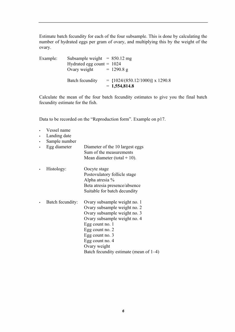
Estimate batch fecundity for each of the four subsample. This is done by calculating the number of hydrated eggs per gram of ovary, and multiplying this by the weight of the ovary. Example: Subsample weight = 850.12 mg Hydrated egg count = 1024 Ovary weight = 1290.8 g Batch fecundity = {1024/(850.12/1000)} x 1290.8 = 1,554,814.8 Calculate the mean of the four batch fecundity estimates to give you the final batch fecundity estimate for the fish. Data to be recorded on the “Reproduction form”. Example on p17. • Vessel name • Landing date • Sample number • Egg diameter Diameter of the 10 largest eggs Sum of the measurements Mean diameter (total ÷ 10). • Histology: Oocyte stage Postovulatory follicle stage Alpha atresia % Beta atresia presence/absence Suitable for batch decundity • Batch fecundity: Ovary subsample weight no. 1 Ovary subsample weight no. 2 Ovary subsample weight no. 3 Ovary subsample weight no. 4 Egg count no. 1 Egg count no. 2 Egg count no. 3 Egg count no. 4 Ovary weight Batch fecundity estimate (mean of 1–4)
6

OOCYTE DESCRIPTIONS
Figure 3: Generalised diagram of an egg (oocyte) surrounded by the granulosa cells, basement membrane and thecal cells. Nucleus is migrating to the margin of the oocyte, signalling the onset of maturation. (Adapted from Takashima and Hibiya, 1995).
OOGENESIS
1 Unyolked stage
Small perinuclear oocytes with purple stained cytoplasm and a spherical nucleus. Peripheral nucleoli (small black dots) may be seen in the nucleus, along with differential staining of the cytoplasm, which might be precursors of yolk vesicles. See figure 4. 20 – 150 µm diameter.
VITELLOGENESIS
2 Early yolked stage
An accumulation of pale purple stained yolk vesicles begins in the cytoplasm. These yolk vesicles initially concentrate at the periphery of the oocyte and spread inwards towards the nucleus. Peripheral nuclei are present. 150 - 300 µm diameter. The whole oocyte takes on a pink colour as yolk granules appear at the periphery replacing the yolk vesicles. Purple stained yolk vesicles are still present near the nuclei. A purple zona radiata is obvious at this stage. See figure 4. 250 - 400 µm diameter.
7

Figure 4. Histological section showing unyolked, early yolked and advanced yolked oocytes.
3 Advanced yolked stage
Pink stained yolk granules (spheres) are present throughout the oocyte. The zona radiata is wide, turns pink and shows radial striations. The nucleus is centrally located. See figure 5. 400 – 700 µm in diameter.
Figure 5. Histological section showing an advanced yolked oocyte.
MATURATION
4 Migratory nucleus stage
The nucleus migrates to the periphery of the oocyte and is usually replaced by a few large oil droplets (figure 6 and 7). Sometimes you can see the yolk granules fusing to form yolk plates (See figure 8). It is rare to see the nuclei right at the edge of the oocyte, but the large central oil droplets usually tell you it is at migratory nucleus stage. Migratory nucleus stage is also very short-lived and may only occur at a certain time of day. The oocyte enlarges to approx. 550 - 800 µm diameter.
8

Figure 6. Histological section showing a migratory nucleus oocyte.
Figure 7. Histological section showing a migratory nucleus oocyte.
Figure 8. Histological section showing a migratory nucleus oocyte, with visible yolk plates.
5 Hydrated stage
The yolk coalesces completely (uniform pink stain). The oocyte significantly increases in size and appears irregular in shape (probably due to a loss of fluid during histological preparation) with no of very few fat vesicles. As the oocyte expands the zona radiata is stretched into a thin band. See figures 9 and 10. Diameter is approx. 800 to 1200 µm diameter.
9

Figure 9. Histological section showing hydrated oocyte.
Figure 10. Histological section showing hydrated oocyte.
10
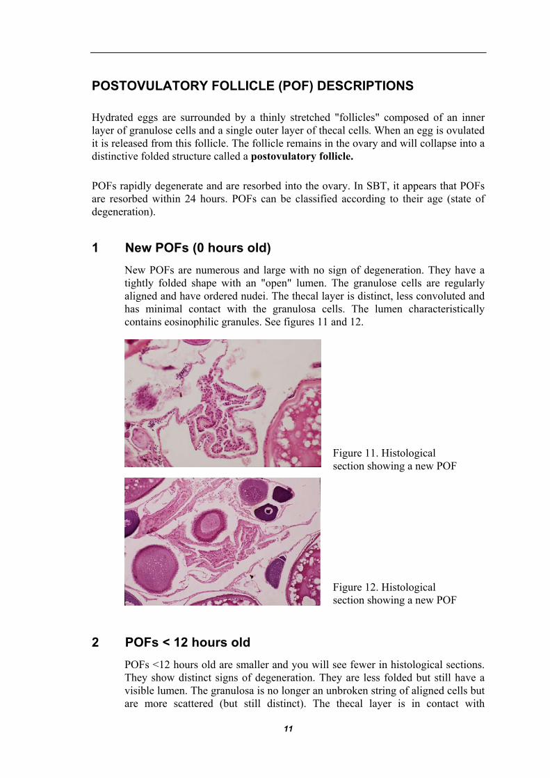
POSTOVULATORY FOLLICLE (POF) DESCRIPTIONS
Hydrated eggs are surrounded by a thinly stretched "follicles" composed of an inner layer of granulose cells and a single outer layer of thecal cells. When an egg is ovulated it is released from this follicle. The follicle remains in the ovary and will collapse into a distinctive folded structure called a postovulatory follicle.
POFs rapidly degenerate and are resorbed into the ovary. In SBT, it appears that POFs are resorbed within 24 hours. POFs can be classified according to their age (state of degeneration).
1 New POFs (0 hours old) New POFs are numerous and large with no sign of degeneration. They have a tightly folded shape with an "open" lumen. The granulose cells are regularly aligned and have ordered nudei. The thecal layer is distinct, less convoluted and has minimal contact with the granulosa cells. The lumen characteristically contains eosinophilic granules. See figures 11 and 12.
Figure 11. Histological section showing a new POF
Figure 12. Histological section showing a new POF
2 POFs < 12 hours old POFs <12 hours old are smaller and you will see fewer in histological sections. They show distinct signs of degeneration. They are less folded but still have a visible lumen. The granulosa is no longer an unbroken string of aligned cells but are more scattered (but still distinct). The thecal layer is in contact with
11

granulosa layer. The lumen may still contain eosinophilic granules. See figure 13.
Figure 13. Histological sectionshowing a POF <12 hours old
3 POFs 12 - 24 hours old POFs are smaller, lack folds and are generally elongate. The lumen is veIy small and eosinophilic granules cannot be seen.The thecal layer is still present, but much thinner and is in complete contact with the granulosa. The granulosa now consists of fewer cells, pycnotic nudei and vacuoles. See figure 14.
Figure 14. Histological section showing a POF 12 – 24 hours old
12

ATRETIC OOCYTE DESCRIPTIONS
Atresia is the resorption of fully yolked oocytes and their follicles. Atresia is divided into alpha (the initial phase) and beta (the latter stage).
1 Alpha atresia
During alpha atresia, the yolk granules are broken down and the granulosa enlarges. The oocyte has a disorganised appearance. The oocytes are stained a lighter pink colour, compared to non-atretic oocytes. See figure 15 and 16.
Figure 15. Histological section showing an oocyte in the early alpha phase of atresia.
Figure 16. Histological section showing an oocyte in the late alpha phase of atresia.
2 Beta atresia
During beta atresia, the yolk granules are broken down even further. The oocyte has a “spider web” appearance. Beta atresia oocytes are composed of granulosa cells with intracellular vacuoles. Blood vessels are commonly associated with these structures. See figure 17 and 18.
13

Figure 17. Histological section showing an oocyte in the early beta phase of atresia.
Figure 18. Histological section showing an oocyte in the late beta phase of atresia.
14

DECAYING OVARY TISSUE
It can be difficult to distinguish between normal ovary tissue and tissue that may be showing signs of decay. Decay can begin if the ovary has been left too long ‘on ice’ (either on the vessel or in the processing plant). If decay has begun, it may be difficult to distinguish postovulatory follicles. These ovaries must be identified. Figures 19 and 20 show ovaries in advanced states of decay. Usually, decaying ovaries can be distinguished by the presence of stained material (not clear) between the follicle (granulosa and thecal cells) and the zona radiata, and between the eggs.
Figure 19. Eggs in an ovary that appears to be decaying. Note: this is a histologicalsection from an ovary that was frozen prior to fixation.
Stainedmaterial
Figure 20. Eggs in an ovary that appears to be decaying.
15

DATA ENTRY FORMS
1 SBT ovary form
16

2 Reproduction form
17

REFERENCES
Farley, J.H. and Davis, T.L.O. 1998.
Reproductive dynamics of southern bluefin tuna, Thunnus maccoyii. Fishery Bulletin 96: 223-236.
Takashima, F. and Hibiya, T. 1995.
An atlas of fish histology, normal and pathological features. Kodansha Ltd, Tokyo, Japan, p 129.
18