SINGLE CHANNEL SPEECH ENHANCEMENT USING

KALMAN FILTER

Sujan Kumar Roy

A thesis

in

The Department

of

Electrical and Computer Engineering

Presented in Partial Fulfillment of the Requirements

For the Degree of Master of Applied Science

Concordia University

Montreal, Quebec, Canada

January 2016

c© Sujan Kumar Roy, 2016

Concordia UniversitySchool of Graduate Studies

This is to certify that the thesis prepared

By: Sujan Kumar Roy

Entitled: Single Channel Speech Enhancement Using Kalman Fil-

ter

and submitted in partial fulfillment of the requirements for the degree of

Master of Applied Science

complies with the regulations of this University and meets the accepted standards

with respect to originality and quality.

Signed by the final examining commitee:

Dr. R. Raut

Chair

Dr. Y.M. Zhang (MIE)

Examiner, External

to the Program

Dr. M. A. Amer

Examiner

Dr. W-P. Zhu

Supervisor

Dr. W.E. Lynch, Chair

Approved byDepartment of Electrical and Computer Engineering

20

Dr. Amir Asif, Dean

Faculty of Engineering and Computer Science

Abstract

Single Channel Speech Enhancement Using Kalman Filter

Sujan Kumar Roy

The quality and intelligibility of speech conversation are generally degraded by the

surrounding noises. The main objective of speech enhancement (SE) is to eliminate

or reduce such disturbing noises from the degraded speech. Various SE methods have

been proposed in literature. Among them, the Kalman filter (KF) is known to be an

efficient SE method that uses the minimum mean square error (MMSE). However,

most of the conventional KF based speech enhancement methods need access to clean

speech and additive noise information for the state-space model parameters, namely,

the linear prediction coefficients (LPCs) and the additive noise variance estimation,

which is impractical in the sense that in practice, we can access only the noisy speech.

Moreover, it is quite difficult to estimate these model parameters efficiently in the

presence of adverse environmental noises. Therefore, the main focus of this thesis is to

develop single channel speech enhancement algorithms using Kalman filter, where the

model parameters are estimated in noisy conditions. Depending on these parameter

estimation techniques, the proposed SE methods are classified into three approaches

based on non-iterative, iterative, and sub-band iterative KF.

In the first approach, a non-iterative Kalman filter based speech enhancement

algorithm is presented, which operates on a frame-by-frame basis. In this proposed

method, the state-space model parameters, namely, the LPCs and noise variance, are

estimated first in noisy conditions. For LPC estimation, a combined speech smoothing

and autocorrelation method is employed. A new method based on a lower-order

truncated Taylor series approximation of the noisy speech along with a difference

operation serving as high-pass filtering is introduced for the noise variance estimation.

The non-iterative Kalman filter is then implemented with these estimated parameters

effectively.

In order to enhance the SE performance as well as parameter estimation accuracy

in noisy conditions, an iterative Kalman filter based single channel SE method is

iii

proposed as the second approach, which also operates on a frame-by-frame basis.

For each frame, the state-space model parameters of the KF are estimated through

an iterative procedure. The Kalman filtering iteration is first applied to each noisy

speech frame, reducing the noise component to a certain degree. At the end of this

first iteration, the LPCs and other state-space model parameters are re-estimated

using the processed speech frame and the Kalman filtering is repeated for the same

processed frame. This iteration continues till the KF converges or a maximum number

of iterations is reached, giving further enhanced speech frame. The same procedure

will repeat for the following frames until the last noisy speech frame being processed.

For further improving the speech enhancement performance, a sub-band iterative

Kalman filter based SE method is also proposed as the third approach. A wavelet

filter-bank is first used to decompose the noisy speech into a number of sub-bands.

To achieve the best trade-off among the noise reduction, speech intelligibility and

computational complexity, a partial reconstruction scheme based on consecutive mean

squared error (CMSE) is proposed to synthesize the low-frequency (LF) and high-

frequency (HF) sub-bands such that the iterative KF is employed only to the partially

reconstructed HF sub-band speech. Finally, the enhanced HF sub-band speech is

combined with the partially reconstructed LF sub-band speech to reconstruct the

full-band enhanced speech.

Experimental results have shown that the proposed KF based SE methods are

capable of reducing adverse environmental noises for a wide range of input SNRs,

and the overall performance of the proposed methods in terms of different evaluation

metrics is superior to some existing state-of-the art SE methods.

iv

I dedicate this work to my parents...

v

Acknowledgments

First of all, I would like to express my sincerest gratitude and appreciation to my

supervisor, Prof. Wei-Ping Zhu, for providing me with financial aid and the unique

opportunity to work in the area of speech enhancement, for his expert guidance and

mentorship, and for his encouragement and support at all levels of my research. I am

also grateful to him for including me in the NSERC CRD research project sponsored

by Microsemi.

I would like to give special thanks to Prof. Benoit Champagne, McGill University,

Canada for his consistent support, valuable comments and suggestions during my

M.A.Sc thesis and the CRD project research. I would also like to give special thanks

to the Microsemi technical staff for their inputs and feedbacks on my research during

the regular project progress meetings.

I am also grateful to my research team mates, Mr. Mahdi Parchami, and Mr.

Xinrui Pu, and all my signal processing laboratory members for their assistance,

friendship, and cooperation. Their smile and support motivated me during this re-

search and gave me the taste of a family in Canada.

I am also grateful to Concordia University for providing me with the GSSP fund-

ing and the conference grant during my M.A.Sc study, which helped me to attend the

2014 Canadian Conference on Electrical and Computer Engineering (CCECE), held

in Toronto, Canada.

At last but not the least, I would like to thank my family members for their

life-long love and support without boundaries, which have always been a source of

motivation and happiness for me.

vi

Contents

List of Figures x

List of Tables xiv

List of Abbreviations xv

List of Symbols xvi

1 Introduction 1

1.1 Overview of Speech Enhancement . . . . . . . . . . . . . . . . . . . . 1

1.1.1 Categories of Speech Enhancement Algorithm . . . . . . . . . 3

1.1.2 Statistical Properties of Different Additive Noises . . . . . . . 4

1.2 Literature Review . . . . . . . . . . . . . . . . . . . . . . . . . . . . . 6

1.2.1 Time-Domain Speech Enhancement Algorithms . . . . . . . . 6

1.2.1.1 Speech Enhancement using LPC . . . . . . . . . . . 6

1.2.1.2 Speech Enhancement using Kalman Filter . . . . . . 8

1.2.2 Transform-Domain Speech Enhancement Algorithms . . . . . 10

1.2.2.1 Speech Enhancement using Spectral Subtraction . . 11

1.2.2.2 Speech Enhancement using Wiener Filtering . . . . . 13

1.2.2.3 Speech Enhancement using Wavelet . . . . . . . . . . 14

1.3 Motivation . . . . . . . . . . . . . . . . . . . . . . . . . . . . . . . . . 16

1.4 Objective of the Thesis . . . . . . . . . . . . . . . . . . . . . . . . . . 17

1.5 Organization of the Thesis . . . . . . . . . . . . . . . . . . . . . . . . 18

2 Speech Enhancement using Kalman Filter 20

2.1 Introduction . . . . . . . . . . . . . . . . . . . . . . . . . . . . . . . . 20

2.2 Human Speech Modeling using LPC Analysis . . . . . . . . . . . . . 21

vii

2.2.1 Conventional LPC Estimation in Noise-free Case . . . . . . . 24

2.2.2 Existing LPC Estimation Methods in Noisy Conditions . . . . 26

2.3 Conventional Kalman Filter for Speech Enhancement . . . . . . . . . 27

2.4 Proposed Non-Iterative Kalman Filter based Speech Enhancement . . 32

2.4.1 Proposed Noise Variance Estimation Algorithm . . . . . . . . 34

2.4.2 Proposed LPC Estimation Algorithm . . . . . . . . . . . . . . 36

2.5 Proposed Speech Enhancement Algorithm using Iterative Kalman Filter 39

2.6 Performance Comparisons of the Proposed Methods . . . . . . . . . . 44

2.7 Conclusion . . . . . . . . . . . . . . . . . . . . . . . . . . . . . . . . . 45

3 Proposed Speech Enhacement Algorithm using Sub-band Iterative

Kalman Filter 47

3.1 Introduction . . . . . . . . . . . . . . . . . . . . . . . . . . . . . . . . 47

3.2 Wavelets and Filter-bank . . . . . . . . . . . . . . . . . . . . . . . . . 48

3.2.1 Two-channel Filter-bank Structure . . . . . . . . . . . . . . . 50

3.2.2 Perfect Reconstruction of Two-channel Filter-bank . . . . . . 51

3.2.3 M-channel Filter-bank . . . . . . . . . . . . . . . . . . . . . . 53

3.3 Proposed Speech Enhancement Algorithm using Sub-band iterative

Kalman Filter . . . . . . . . . . . . . . . . . . . . . . . . . . . . . . . 54

3.3.1 CMSE Based Synthesis . . . . . . . . . . . . . . . . . . . . . . 56

3.3.2 Proposed Sub-band Iterative Kalman Filter . . . . . . . . . . 58

3.3.3 Parameter Estimation . . . . . . . . . . . . . . . . . . . . . . 60

3.4 Performance of the Proposed Method . . . . . . . . . . . . . . . . . . 61

3.5 Conclusion . . . . . . . . . . . . . . . . . . . . . . . . . . . . . . . . . 64

4 Simulation Results and Discussions 65

4.1 Experimental Setup . . . . . . . . . . . . . . . . . . . . . . . . . . . . 65

4.2 Performance Evaluation Methods . . . . . . . . . . . . . . . . . . . . 66

4.3 Performance Comparisons between the Proposed and Existing Methods 68

4.4 Comprehensive Performance Comparisons between the Proposed Meth-

ods . . . . . . . . . . . . . . . . . . . . . . . . . . . . . . . . . . . . . 72

4.5 Computational Complexity . . . . . . . . . . . . . . . . . . . . . . . . 79

4.6 Conclusion . . . . . . . . . . . . . . . . . . . . . . . . . . . . . . . . . 82

viii

5 Conclusion 83

5.1 Summary of the Work . . . . . . . . . . . . . . . . . . . . . . . . . . 83

5.2 Suggestions for Future Work . . . . . . . . . . . . . . . . . . . . . . . 85

Bibliography 86

ix

List of Figures

1.1 Block diagram of single channel speech enhancement. . . . . . . . . . 4

2.1 The anatomy of human speech production system. . . . . . . . . . . . 21

2.2 Source filter model of human speech production system. . . . . . . . . 22

2.3 Linear prediction model for human speech production. . . . . . . . . 22

2.4 All-pole filtering system for speech production . . . . . . . . . . . . . 23

2.5 Estimation of residual error ε[n] using the prediction filter. . . . . . . 24

2.6 Performance comparison between the original and the estimated noise

variance, (a) non-stationary noise, (b) restaurant noise experiment.

Speech samples are taken from the TIMIT database (input SNR=0dB). 35

2.7 (a) clean speech (male) frame, (b) white noise (input SNR=5dB) cor-

rupted frame, and is the corresponding smoothed speech frame. . . . 37

2.8 (a) clean speech (female) frame, (b) non-stationary noise (input SNR=5dB)

corrupted frame, and is the corresponding smoothed speech frame. . . 37

2.9 Power spectra comparison between the clean speech (dashed), degraded

speech (dotted), and estimated speech (solid), in the presence of non-

stationary noise (Input SNR= 0dB). . . . . . . . . . . . . . . . . . . 40

2.10 Power spectra comparison between the clean speech (dashed), degraded

speech (dotted), and estimated speech (solid), in the presence of pink

noise (Input SNR = 0dB). . . . . . . . . . . . . . . . . . . . . . . . . 40

2.11 Power spectra comparison between the clean speech (magenta), de-

graded speech (red), estimated(NIT-KF) (black), and estimated(IT-

KF) (blue) in presence of the non-stationary noise (Input SNR = 0dB). 43

2.12 Power spectra comparison between the clean speech (magenta), de-

graded speech (red), estimated(NIT-KF) (black), and estimated(IT-

KF) (blue) in the presence of the pink noise (Input SNR = 0dB). . . 43

x

2.13 Performance comparison between the proposed methods and other ex-

isting competitive methods in terms of PESQ. The speech utterances

are corrupted by (a): White, (b): Babble and (c): Car noises for a

wide range of input SNRs(-10dB to 15dB). . . . . . . . . . . . . . . . 45

3.1 (a) Block diagram of an M -channel filter-bank structure, and (b) ap-

proximate frequency responses of analysis filters. . . . . . . . . . . . . 49

3.2 (a) Block diagram of a simple two-channel filter-bank structure, and

(b) approximate frequency responses of analysis filters. . . . . . . . . 50

3.3 A four-level wavelet packet tree decomposition structure. . . . . . . . 53

3.4 Block-diagram of the proposed sub-band iterative Kalman filter for

single channel speech enhancement. . . . . . . . . . . . . . . . . . . . 55

3.5 (a) Speech sample (TIMIT database) corrupted by babble noise (SNR=10dB),

(b) the corresponding 16 reconstructed subbands. . . . . . . . . . . . 56

3.6 The CMSE values corresponding to the sub-band speeches in Fig. 3.5.

The double circle indicates the js. . . . . . . . . . . . . . . . . . . . . 57

3.7 Power spectra comparison between the clean speech (solid), degraded

speech (dotted), and estimated (SBIT-KF) speech (dashed) in the pres-

ence of babble noise (SNR = 0dB). . . . . . . . . . . . . . . . . . . . 61

3.8 Performance comparison between the original and estimated noise vari-

ances obtained from the partially reconstructed sub-band speech yh(n)

and full-band noisy speech y(n), respectively, (a) white Gaussian, (b)

non-stationary noise experiment. Speech utterances are taken from the

TIMIT database (input SNR=-5dB). . . . . . . . . . . . . . . . . . . 62

3.9 Performance comparison between the proposed methods and other ex-

isting competitive methods in terms of PESQ. The speech utterances

are corrupted by (a): White, (b): Babble and (c): Car noises for a

wide range of input SNRs(-10dB to 15dB). . . . . . . . . . . . . . . . 63

4.1 Simplified block-diagram of the PESQ evaluation. . . . . . . . . . . . 66

4.2 Performance comparison between the proposed and existing competi-

tive methods in terms segmental SNR (dB). The speech utterances are

corrupted by (a): White, (b):F16 Cockpit, and (c): Babble noises for

a wide range for input SNRs(-10dB to 15dB). . . . . . . . . . . . . . 69

xi

4.3 Performance comparison between the proposed and existing methods

in terms of PESQ. The speech utterances are corrupted by (a): White,

(b): F16 Cockpit, and (c): Babble noises for a wide range for input

SNRs(-10dB to 15dB). . . . . . . . . . . . . . . . . . . . . . . . . . . 69

4.4 Performance comparison between the proposed and other existing meth-

ods in terms of segmental SNR (dB). The speech utterances are cor-

rupted by (a): Car, (b):Street, (c): Train, and (d): Restaurant noises

for a wide range of input SNRs(0dB to 15dB). . . . . . . . . . . . . . 71

4.5 Performance comparison between the proposed and other existing meth-

ods in terms of PESQ. The speech utterances are corrupted by (a): Car,

(b): Street, (c): Train, and (d): Restaurant noises for a wide range of

input SNRs(0dB to 15dB). . . . . . . . . . . . . . . . . . . . . . . . . 71

4.6 Spectrograms of (a): clean speech, (b): noisy speech, and enhanced

speech (c,d,e) obtained through using the Proposed-NIT-KF, Proposed-

IT-KF, and Proposed-SBIT-KF, respectively in the presence of white

Gaussian noise (input SNR=5dB). . . . . . . . . . . . . . . . . . . . . 73

4.7 Spectrograms of (a): clean speech, (b): noisy speech, and enhanced

speech (c,d,e) obtained through using the Proposed-NIT-KF, Proposed-

IT-KF, and Proposed-SBIT-KF, respectively in the presence of non-

stationary noise (input SNR=5dB). . . . . . . . . . . . . . . . . . . . 74

4.8 Performance comparison between the proposed methods in terms of

segmental SNR (dB) for a wide range of input SNRs (-10dB to 15dB)

in the presence of 9 types of noises. . . . . . . . . . . . . . . . . . . . 75

4.9 Performance comparison between the proposed methods in terms of

PESQ for a wide range of input SNRs (-10dB to 15dB) in the presence

of 9 types of noises. . . . . . . . . . . . . . . . . . . . . . . . . . . . . 76

4.10 Performance comparison between the proposed methods in terms of

output SNR (dB) for a wide range of input SNRs (-10dB to 15dB) in

the presence of 9 types of noises. . . . . . . . . . . . . . . . . . . . . . 77

4.11 Performance comparison between the proposed methods in terms of

LLR for a wide range of input SNRs (-10dB to 15dB) in the presence

of 9 types of noises. . . . . . . . . . . . . . . . . . . . . . . . . . . . . 78

xii

4.12 Computational complexity comparison of the proposed methods, (a):

CPU time (sec) versus LPC order and (b): PESQ versus LPC order in

the presence of restaurant noise (input SNR=10dB). . . . . . . . . . . 81

xiii

List of Tables

1 Derivative Templates. . . . . . . . . . . . . . . . . . . . . . . . . . . . 34

2 Different Smoothing Kernels . . . . . . . . . . . . . . . . . . . . . . . 36

xiv

List of Abbreviations

ACF Autocorrelation function

AR Auto-regressive

ARMA Auto regressive moving average

ASR Automatic Speech Recognition

CMSE Consecutive mean squared error

DCT Discrete cosine transform

DFT Discrete Fourier transform

DWT Discrete wavelet transformation

EM Expectation maximization

FIR Finite impulse response

HF High-frequency

IT-KF Iterative Kalman filter

IDFT Inverse discrete Fourier transformation

IWF iterative Wiener filter

KF Kalman filter

LF Low-frequency

LLR Log-likelihood ratio

LP Linear prediction

LPC Linear prediction coefficient

PR Perfect reconstruction

MAP Maximum a-posteriori

MMSE minimum mean square error

MSE Mean squared error

NIT-KF Non-iterative Kalman filter

PESQ Perceptual evaluation of speech quality

SE Speech enhancement

SNR Signal-to-noise ratio

SSM State-space model

WF Wiener filter

WFB Wavelet filter-bank

xv

List of Symbols

s(n) Clean speech

y(n) Noisy speech

u(n) Process noise

v(n) Additive noise

s(n) Enhanced speech

AP (z) All-pole filter

x(t) Excitation signal

ε(n) Prediction error

Rss Autocorrelation matrix of clean speech s(n)

A LPC vector

Φ Transition matrix

Σx Covariance matrix

e(n) Measurement innovation

K(n) Kalman gain

Tr() Trace operator

E. Expectation operator

σ2v Additive Noise Variance

σ2u Process Noise Variance

x(n|n) State vector

sh(n) Partially reconstructed HF sub-band speech

sl(n) Partially reconstructed LF sub-band speech

js Last HF sub-band index

xvi

Chapter 1

Introduction

1.1 Overview of Speech Enhancement

Speech enhancement is essential in modern voice communication systems. Speech

communication devices like cellular phones, handsfree equipment, human-to-machine

speech processing systems, etc. are an integral part of our daily life. In real-life, the

speech communication takes place in different noisy environments where the original

clean speech could be degraded due to the presence of surrounding noises. These

noises can range from stationary white noise to any non-stationary and/or colored

noises such as street noise, car engine noise, babble noise, restaurant noise, etc. In

many speech communication and processing systems, the desired clean speech is not

available due to degradation by the ambient noises [1]. Therefore, noise reduction of

speech has been an active area of research over the last few decades.

The performance of speech enhancement algorithms is evaluated according to the

quality and intelligibility of the enhanced speech. In general, speech quality assess-

ment falls into two categories; subjective and objective quality measures. Subjective

quality measures are based on comparison of original and enhanced speech by a lis-

tener or a panel of listeners, where they rank the quality of the enhanced speech

according to a predetermined scale. Objective quality measures are calculated from

the original speech and the processed speech using some mathematical formulas. On

the other hand, speech intelligibility is another quality measure to indicate how com-

prehensible a speech is in given conditions. The relationship between speech quality

and intelligibility is not entirely understood, yet there exists some correlation between

1

these two. Generally, speech perceived as good quality gives high intelligibility, and

vice versa. However, there are speech samples that are rated as poor quality, and yet

give high intelligibility, and vice versa [2]. Therefore, it is very important for a SE

algorithm to maintain good quality as well as intelligibility of the enhanced speech.

Speech enhancement has been widely used as a front end tool for automatic speech

recognition, telecommunications, hearing aids, etc. By improving the quality and in-

telligibility of the degraded speech using a SE method, it vastly improves the listening

experience of users through these consumer applications. A brief description of speech

enhancement applications is given below.

Automatic Speech Recognition: Automatic Speech Recognition (ASR) has

been an important field of research since the 1950s. It can recognize human

spoken words or sentences, and thus has many important real-world applica-

tions including person identification, human-robot communication, etc. The

key requirement of these applications is to distinguish between similar sounding

words. However, in practical applications, the speech recognition accuracy be-

comes degraded due to the sorrounding noise. SE in such situations is used as a

front end tool of the ASR system to remove the unwanted noises or other inter-

ferences in the speech samples before the ASR software attempts to recognize

the speech [3].

Telecommunications: One of the important applications of speech enhance-

ment found in telecommunication systems is specifically mobile or cellular tele-

phony. Due to the majority of the cell phone conversations taking place in

noisy environments, namely automobiles, streets or public places, noise will in-

evitably be mixed up with the speech, making the conversation disturbing for

the listener. A speech enhancement algorithm plays an important role in order

to remove these unwanted noises, making the public conversation through cell

phones more efficient [4].

Hearing Aids: The hearing aid devices consist of a microphone and amplifier

including some DSP hardware. It is used by hearing impaired people. In ad-

verse acoustic environments, individuals with hearing impairment may struggle

to understand the speech content due to the interfering sounds, background

noise, and reverberation. Like any other microphone, this is susceptible to

2

picking up unwanted noise along with the speech. Therefore, a robust speech

enhancement algorithm programmed on the DSP chip may improve the users

listening experience [4].

Other Applications: In audio recording industry, speech enhancement plays a

key role in removing different interferences like acoustic echo and reverberation.

It is also used in air-ground communication, emergency equipment like elevator,

SOS alarm, vehicular emergency telephones, VoIP, etc.

1.1.1 Categories of Speech Enhancement Algorithm

Speech enhancement algorithms are implemented based on certain assumptions de-

pending on different applications. In general, these algorithms are classified based

on the number of input channels or microphones (single/multiple microphones), and

the domain of processing (time/transform domain). The time-domain or transform-

domain speech enhancement algorithms can also be further classified as adaptive and

non-adaptive depending on parameter estimation. In the single channel speech en-

hancement algorithm, one noisy mixture gives the overall spectral information of the

degraded speech since there is only one microphone/channel available. On the other

hand, in multi-channel speech enhancement, multiple microphones are available in

order to capture the noisy mixtures which exhibit the advantage of incorporating

both the spatial and the spectral information. However, multi-channel systems in-

crease the system implementation costs and may not always be available. Therefore,

single channel speech enhancement is of more interest in many speech processing

applications [5].

The main focus of this thesis is to implement efficient single channel speech en-

hancement that can perform well in the presence of adverse environmental noises.

For a single microphone speech s(n), and additive noise v(n) which may be white or

colour noise, the noise corrupted speech signal y(n) at time n is then represented as

y(n) = s(n) + v(n) (1.1)

The general block diagram of single channel SE is shown in Figure 1.1, where the

SE algorithm is to estimate the clean speech s(n) from the noisy speech y(n).

3

Figure 1.1: Block diagram of single channel speech enhancement.

1.1.2 Statistical Properties of Different Additive Noises

The main objective of speech enhancement algorithm is to estimate the clean speech

s(n) from the noise corrupted speech y(n) through different noise reduction algo-

rithms. However, it is a challenging task to eliminate or reduce the additive noise

v(n) in the noisy observation due to the random nature of the noise and the intrinsic

complexities of the clean speech s(n). In addition, different noises possess different

statistical characteristics. Due to this reason, a speech enhancement algorithm may

perform well for a particular type of noise, but not efficient for other types of noises.

Therefore, it is important to understand the statistical characteristics of the additive

noise v(n) in order to develop an efficient speech enhancement algorithm for differ-

ent environmental noises. Depending on the time or frequency characteristics, the

additive noise v(n) in (1.1) can be classified into the following categories.

• White Noise: It is defined as an uncorrelated noise process with a constant

power spectral density. It is a wide-band noise which theoretically contains all

frequencies within the signal bandwidth.

• Non-stationary Noise: In non-stationary noise, the power spectral density is

not constant and changes over time. It is quite difficult to deal with this noise,

since there is no prior information available about the characteristics of that

noise.

• Pink Noise: Pink noise is a type of noise where the power spectral density

(energy or power per Hz) is inversely proportional to the frequency of the signal.

Therefore, the lower frequency components in pink noise have more power than

the higher frequencies.

4

• Restaurant Noise: This type of noise contains multiple people talking in the

background mixed in some cases with other noises coming from the kitchen

or other utensil sounds. The spectral characteristics of restaurant noise are

randomly changing as people carry on conversation to the neighbouring tables

or the waiters interaction with guests during services.

• Babble Noise: This type of noise is encountered when a crowd or a group of

people are talking together simultaneously (i.e. in a cafeteria, crowded class-

room, or other places). It has the characteristics of time varying amplitudes.

In addition, some of the noise frequencies may coincide closely with the original

clean speech samples.

• Street Noise: The street noise includes vehicle’s engine sound and other ex-

haust noise which increases with vehicle speed. The amplitude of this type of

noise also changes rapidly.

• Car Noise: This type of noise contains car interior and engine sound during

conversation through cell phone or other communication devices. It may also

include break sound, tyre sound, and other exhaust sounds.

• Train Noise: Train noise contains its interior sounds, several distinct sounds

such as the locomotive engine noise, and the wheels turning on the railroad

track. It may also include horns, whistles, bells, and other noisemaking devices

for both communication and warning.

• Cockpit Noise: This type of noise includes plane interior sound, engine sounds,

and other exhaust sounds which may take place during the radio communica-

tion between the pilot and the air-traffic controller. This type of noise spectra

may vary greatly as a function of the aircraft size and type and other associated

parameters.

In general, speech enhancement algorithm can be thought of as an estimation

problem, where an unknown signal (clean speech) is to be estimated in the presence

of different types of noises, where only the noisy observation is available. Therefore,

it is quite difficult for a particular speech enhancement algorithm to perform well

across different types of noises [6].

5

1.2 Literature Review

Research on speech enhancement started more than 40 years ago at AT & T Bell Lab-

oratories, with the pioneering work by Schroeder as mentioned in [7]. Schroeder pro-

posed an analog implementation (consisting of bandpass filters, rectification and av-

eraging circuitry) of spectral magnitude subtraction method for speech enhancement.

Although there are many speech enhancement algorithms available nowadays, sev-

eral existing algorithms (time-domain/transform- domain) for single channel speech

enhancement are reviewed in this section which are closely related to this thesis, and

will be implemented for comparison purposes.

1.2.1 Time-Domain Speech Enhancement Algorithms

Time-domain linear filtering approach for single channel SE is a popular one nowa-

days. In this approach, the SE problem is formulated as a filter design problem. More

specifically, a filter should be designed such that it can reduce the additive noise level

of the noisy speech as much as possible while not introducing any noticeable dis-

tortion in the enhanced speech [8]. Different types of linear filters can be designed

in time-domain. One example of such an approach is the AR model based human

speech production system. This model uses all-pole synthesis filtering techniques for

estimating the LPC in noisy conditions. With the estimated LPCs, the approximated

clean speech samples can be modeled. Kalman filter is also commonly used as a time-

domain single channel speech enhancement method. The following subsections briefly

review these important time-domain speech enhancement algorithms.

1.2.1.1 Speech Enhancement using LPC

LPC based speech enhancement algorithms can be thought of as a linear time varying

system which is modelled by a digital filter with time-varying coefficients. In this type

of noise reduction algorithms, the speech samples are represented by P th order auto-

regressive (AR) model, where the speech production model parameters, namely, the

LPCs are estimated from the noise corrupted speech [9].

Lim and Oppenheim in [10] introduced an LPC model based iterative scheme for

enhancing the noise corrupted speech. These algorithms are based on the assumption

of Gaussian excitation of the maximum a-posteriori (MAP) estimator where the LPC

6

parameters are obtained from the clean speech. However, in noisy condition, the

equations for solving the MAP estimator becomes non-linear which is difficult to solve.

The authors of [10] suggested an iterative procedure which requires only a solution of

a set of linear equations for LPC parameter estimation from noisy observations. This

iterative procedure is referred to as linearized MAP (LMAP). This algorithm requires

an initial estimate of the LPC parameters from noisy speech and then enhances the

noisy speech by an appropriate application of an optimal filter. Then a new estimate

of the LPC parameters is obtained by using the autocorrelation based method which

is more accurate. The estimated speech samples are modeled with these new set of

LPCs. The authors obtained the preliminary results of the enhanced speech after 2-3

iterations, where the formant bandwidth becomes very narrow, giving an unnatural

sound and distorted estimated speech.

An improvement of LPC for noise reduction based on pitch synchronous addition

method has been presented in [11]. It resolved the LPC estimation problem in noisy

conditions. The idea is based on that the speech has a valid pitch period, which

may hold up to 20-25 milliseconds for one utterance, and the speech is assumed to

be stationary within this period. In addition, the amplitude of the waveform of the

benchmark speech within each period remains constant. Using this property of speech,

the authors synchronized the pitch period by applying the averaging operation which

decreases the noise power if the speech samples are corrupted by an additive noise.

Therefore, more accurate LPCs can be estimated from the processed speech which

can guarantee the stability of the all-pole synthesis filter during LPC estimation. One

shortcoming of this method is that it requires to estimate accurate pitch period in

order to perform pitch synchronous operation, which is relatively difficult in noisy

conditions.

The key point of LPC based speech enhancement is that the LPCs can be esti-

mated accurately if the clean speech is available. In noisy conditions, however, the

estimation of the LPCs becomes a very difficult task. In addition, the all-pole syn-

thesis filter may not be stable in noisy conditions, which is an important condition

for accurate LPC estimation. To overcome this shortcoming, numerous methods have

been proposed in the literature. Unfortunately, a satisfactory solution for preserving

the stability of the all-pole synthesis filter as well as accurate LPC estimation is never

obtained. On the other hand, LPC can be used as an important model parameter for

7

many speech enhancement methods, such as in Kalman filter where the state-space

model is fromed with the LPCs. Therefore, it is still a demanding task to estimate

LPCs in noisy conditions accurately. The next section gives a brief overview of some

Kalman filter based speech enhancement algorithms.

1.2.1.2 Speech Enhancement using Kalman Filter

The Kalman filter (named after its inventor, Rudolf E. Kalman in 1960), was initially

used for spacecraft, aircraft or other astrological signal analysis [12]. However, in

the last two decades, KF based speech enhancement is an active area of research.

In KF, speech is usually modeled as autoregressive (AR) process and represented in

the state-space domain. The LPC and additive noise variance are two important

parameter for Kalman filter implementation. It has several advantages over other

speech enhancement methods, namely, it can maintain the non-stationary nature of

the speech and does not need to assume the stationary condition within a small

analysis frame as required for the other frequency-domain speech enhancement.

The Kalman filter based speech enhancement was first proposed by Paliwal and

Basu in [13]. In this approach, it was shown that the Kalman filter outperformWiener

filter. However, the performance of the proposed algorithm was limited to reduce only

white Gaussian noise. In this method, the linear prediction coefficients are estimated

from clean speech, before being contaminated by white noise, which is however not

true in practical applications. In [14], a neural network model for speech generation

trained by dual extended Kalman filter was introduced where no justification for the

non-linear system model was given. In [15], an iterative and sequential Kalman filter

based speech enhancement algorithm has been proposed. This algorithm performs

relatively well in terms of output SNR improvement. In addition, the authors of this

paper also used higher-order statistics combindly with the Kalman filter in order to

further improve the performance of the algorithm.

In [16], a Kalman filter based speech enhancement algorithm has been presented

that is capable of reducing color noise. In this paper, new sequential estimation

techniques have been developed for adaptive estimation of the unknown parameters.

A perceptual Kalman filter based speech enhancement method has been proposed in

[17, 18], where the perceptual weighting is used to replace the masking threshold.

It avoids the frequency domain complexity and makes it suitable to estimate the

8

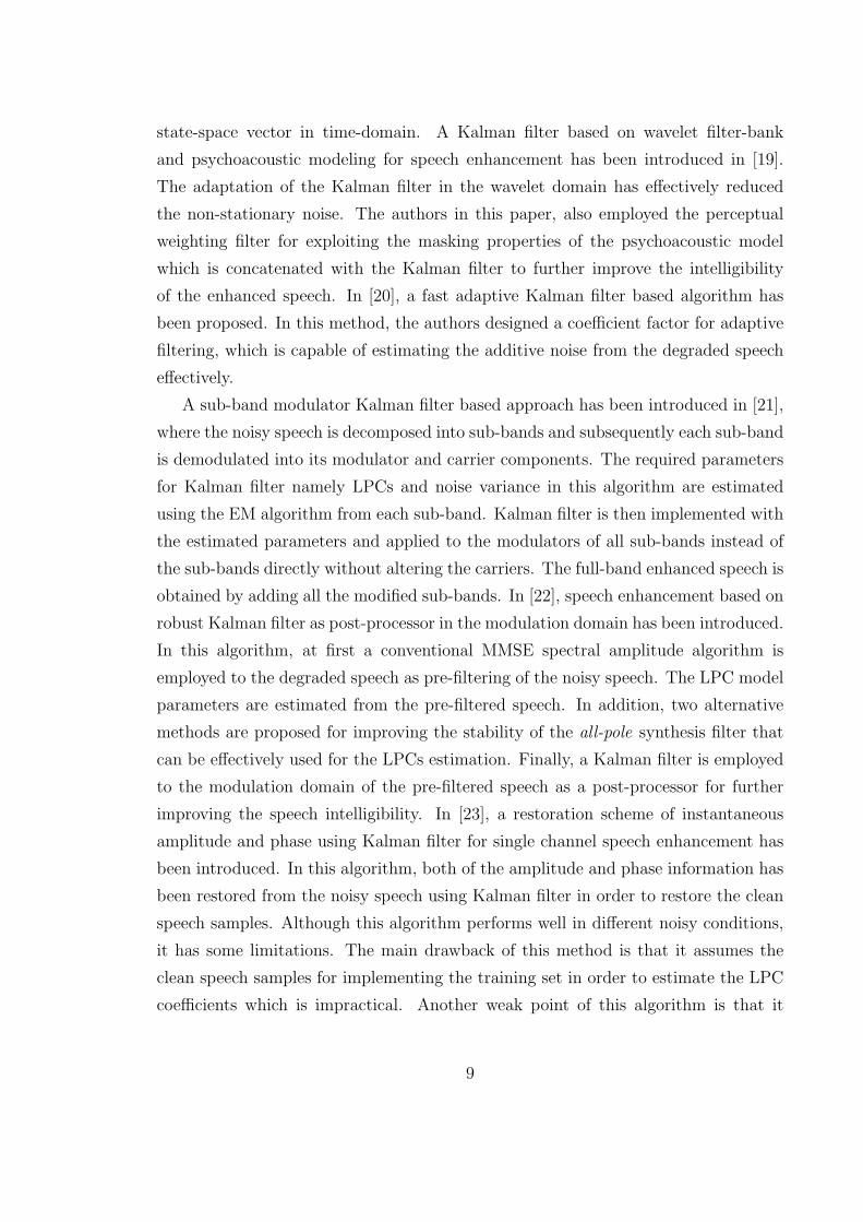
state-space vector in time-domain. A Kalman filter based on wavelet filter-bank

and psychoacoustic modeling for speech enhancement has been introduced in [19].

The adaptation of the Kalman filter in the wavelet domain has effectively reduced

the non-stationary noise. The authors in this paper, also employed the perceptual

weighting filter for exploiting the masking properties of the psychoacoustic model

which is concatenated with the Kalman filter to further improve the intelligibility

of the enhanced speech. In [20], a fast adaptive Kalman filter based algorithm has

been proposed. In this method, the authors designed a coefficient factor for adaptive

filtering, which is capable of estimating the additive noise from the degraded speech

effectively.

A sub-band modulator Kalman filter based approach has been introduced in [21],

where the noisy speech is decomposed into sub-bands and subsequently each sub-band

is demodulated into its modulator and carrier components. The required parameters

for Kalman filter namely LPCs and noise variance in this algorithm are estimated

using the EM algorithm from each sub-band. Kalman filter is then implemented with

the estimated parameters and applied to the modulators of all sub-bands instead of

the sub-bands directly without altering the carriers. The full-band enhanced speech is

obtained by adding all the modified sub-bands. In [22], speech enhancement based on

robust Kalman filter as post-processor in the modulation domain has been introduced.

In this algorithm, at first a conventional MMSE spectral amplitude algorithm is

employed to the degraded speech as pre-filtering of the noisy speech. The LPC model

parameters are estimated from the pre-filtered speech. In addition, two alternative

methods are proposed for improving the stability of the all-pole synthesis filter that

can be effectively used for the LPCs estimation. Finally, a Kalman filter is employed

to the modulation domain of the pre-filtered speech as a post-processor for further

improving the speech intelligibility. In [23], a restoration scheme of instantaneous

amplitude and phase using Kalman filter for single channel speech enhancement has

been introduced. In this algorithm, both of the amplitude and phase information has

been restored from the noisy speech using Kalman filter in order to restore the clean

speech samples. Although this algorithm performs well in different noisy conditions,

it has some limitations. The main drawback of this method is that it assumes the

clean speech samples for implementing the training set in order to estimate the LPC

coefficients which is impractical. Another weak point of this algorithm is that it

9

requires two different AR models in order to represent the amplitude and phase of

the noisy speech which increases the computational complexity.

Gibson et al. in [24] have proposed to extend the use of the Kalman filter by in-

corporating a colored noise model in order to improve the enhancement performances

for certain classes of noise sources. A disadvantage of the above mentioned Kalman

filtering algorithms is that they do not address the model parameter estimation prob-

lem. Another weak point of this method is that the noise variance is estimated during

the silent period of the noisy speech frame which implies that the use of voice activity

detector (VAD) is needed. In [25], a fast converging iterative Kalman filter for speech

enhancement has been introduced. This algorithm provides less residual noise in the

enhanced speech as compared to the iterative scheme of Gibson, et al. [24]. This is

achieved by the use of long and overlapped frames as well as a tapered window with

a large side lobe attenuation for LPC analysis. In [26], iterative Kalman filtering for

speech enhancement using overlapped frames has been introduced. In this paper, the

authors proposed to use the overlapped windows for LPC analysis in order to reduce

the background residual noise as found in the Gibson’s iterative Kalman filter [24].

From the above literature review, it is clearly observed that the performance of

Kalman filter based speech enhancement depends on the accuracy of the LPC and

noise variance estimation in noisy conditions. As such, a key issue in Kalman filter

based methods is to obtain accurate LPCs and noise variance from noisy speech.

1.2.2 Transform-Domain Speech Enhancement Algorithms

In transform-domain speech enhancement algorithms, the noisy speech samples are

transformed into another domain (e.g., frequency domain, wavelet domain, etc.), in

order to extract further details or other hidden information that may not readily be

available in time-domain speech samples. Among different transform-domain speech

enhancement algorithms, frequency-domain algorithms have been well studied over

the past few decades. The main idea of the frequency-domain speech enhancement

involves transforming the noisy speech into the frequency-domain via the discrete

Fourier transform (DFT) and subtracting an estimate of the noise spectrum from

the noisy spectrum, yielding an approximation of the spectrum of the clean speech,

which is then converted back to the time-domain by the inverse DFT [27]. Spectral

subtraction andWiener filter based frequency-domain speech enhancement algorithms

10

are very popular nowadays.

In order to deal with non-stationary noises, sub-band speech enhancement al-

gorithms have also been investigated which works in other transform-domain (e.g.,

wavelet domain, DCT domain, etc.). In these algorithms, the noisy speech is decom-

posed into several critical sub-bands and then the desired information as required for

speech enhancement is effectively estimated from the sub-bands[28]. Many transform-

domain speech enhancement algorithms have been introduced in the last few decades.

Among them, wavelet transform based algorithms for speech enhancement have been

actively studied. Moreover, some speech enhancement algorithms have been intro-

duced with the combination of wavelet filter-bank and other methods. The following

subsections give a brief overview of some of the transform-domain single channel

speech enhancement algorithms.

1.2.2.1 Speech Enhancement using Spectral Subtraction

The earliest and most commonly used method for speech enhancement is magnitude

spectral subtraction. Since speech and noise are considered to be uncorrelated, if

an estimate of the noise spectrum can be obtained for a particular noisy speech

frame, then an estimate of the clean speech spectrum can be calculated by subtracting

the estimated noise spectrum from the noisy spectrum. The estimated clean speech

spectrum is represented as

S(w) = Y (w)− V (w) (1.2)

where S(w) is the estimated frequency spectrum of the clean speech for a given frame,

Y(w) is the noisy spectrum of the same frame, and V(w) is the estimated noise

spectrum. An estimate of the clean speech is recovered by applying the inverse

discrete Fourier transformation (IDFT) to S(w), to give s(n). Since the human ear is

relatively insensitive to phase, the phase angle of the noisy speech can be used when

reconstructing the enhanced speech using IDFT.

Although the spectral subtraction based speech enhancement algorithm is rel-

atively easier to implement, its effectiveness is heavily dependant on the accurate

estimation of the additive noise spectrum of v(n) which is a difficult task. The ma-

jor drawback of this method is that it leaves residual noise with annoying noticeable

tonal characteristics referred to as musical noise when the estimated noise spectrum

is under-subtracted from the noisy spectrum. The enhanced speech also suffers from

11

distortion if the estimated noise spectrum is over-subtracted from the noisy spectrum.

In order to address these issues, several modified spectral subtraction based al-

gorithms have been proposed. In [29], an improved spectral subtraction for speech

enhancement has been introduced that can reduce the musical noise effectively. How-

ever, this algorithm cannot resolve the speech distortion problem. In [30], spectral

subtraction based speech enhancement using an adaptive spectral estimator has been

introduced. In this algorithm, the authors try to reduce themusical noise and improve

the quality of the enhanced speech by increasing the accuracy of the system spectral

estimator. In addition, this algorithm is capable of reducing the stationary noises. In

[31], spectral subtraction method for speech enhancement using an improved a priori

MMSE has been proposed. In this paper, the authors have introduced an adaptive

averaging factor to accurately estimate the a priori SNR for estimation of the addi-

tive noise spectrum. In [32], the authors introduced an improved spectral subtraction

based speech enhancement algorithm that is capable of reducing the non-stationary

noises. The authors in this paper used smooth spectrums to approximate the clean

speech and noisy spectrums with auto-regressive (AR) model and constructed speech

codebook and noise codebook. They employed the spectral subtraction using the

speech and noise entry from codebooks, which obtained from the log-spectral mini-

mization. However, the proposed algorithm can adapt to varying levels of noise only

when speech is present, which is termed as the limitation of this algorithm. In [33],

a multi-band spectral subtraction method based on auditory masking properties for

speech enhancement has been developed. In this algorithm, a weighted recursive av-

eraging method has been used to estimate the noise power spectrum. Finally, the

spectrum of enhanced speech is obtained through a multi-band spectral subtraction

and a gain function computed according to the subtraction factor.

The spectral subtraction based speech enhancement algorithms are popular for

the simplicity of implementation. However, these algorithms have some major limi-

tations. The performance of these algorithms fully depends on the estimation of the

noise spectrum. In different noisy conditions, especially at low input SNRs, it is quite

difficult to estimate the accurate noise spectrum from the degraded speech. Another

weak point of these algorithms is that they require voiced activity detector in order to

estimate the desired noise from the non-speech portion of the analysis speech. In ad-

dition, it is quite difficult for the spectral subtraction based algorithms to remove the

12

musical noise completely. In order to address these issues, Weiner filter based speech

enhancement techniques have been investigated over the past few decades. The next

subsection briefly describes some existing Weiner filter based speech enhancement

methods.

1.2.2.2 Speech Enhancement using Wiener Filtering

Wiener filter for speech enhancement was suggested as an improvement to the spectral

subtraction by Lim and Oppenheim in [10]. In this method, a Wiener gain function

G(w) is calculated first, which is then multiplied with the noisy speech spectrum for

attenuating the noise frequency components more precisely, namely,

S(w) = G(w)Y (w) (1.3)

where G(w) is Wiener filter gain coefficient for a given frequency w which is defined

as

G(w) =|Y (w)|2 − |V (w)|2

|Y (w)|2. (1.4)

Here, G(w) attenuates each frequency component by a certain amount depending

on the power of the noise at that frequency w. If |V (w)|2 = 0, then G(w) = 1 and no

attenuation takes place, i.e. there is no noise component at the frequency w, whereas

if |V (w)|2 = |Y (w)|2, then G(w) = 0 and the frequency component w is completely

nulled. All other values of G(w) between 0 and 1 scale the power of the signal by an

appropriate amount.

In [34], an iterative Wiener filter (IWF) based speech enhancement algorithm has

been proposed, where the complex LPC analysis has been used instead of the con-

ventional LPC analysis. This method can estimate the desired speech spectrum more

accurately, especially at low input SNRs. However, it introduces some background

noise in the enhanced speech. In [35], perceptual Wiener filter based speech enhance-

ment has been proposed, where Wiener filter with self adaptive averaging factor has

been used to estimate a priori SNR for estimating the clean speech speech spec-

tra, which may contain some musical noise. In order to remove the musical noise,

a perceptual weighting filter based on simultaneous and temporal masking effects of

the human auditory system is employed to the processed speech. In addition, an un-

voiced speech enhancement algorithm is also integrated with the scheme to improve

the intelligibility of the enhanced speech. Although this algorithm in general performs

13

well, a little bit distortion was introduced in the enhanced speech. In [36], sub-band

cross-correlation compensated Wiener filter combined with harmonic regeneration for

speech enhancement has been introduced which is capable of reducing the color noises.

In this algorithm, a nonlinear sub-band Bark scale frequency spacing approach has

been used to reduce the additive color noise effectively. It can also restore the original

harmonic features in the enhanced speech that are lost due to the additive noise effect.

In addition, it can also reduce the distortion in the enhanced speech. However, this

algorithm is not suitable for different adverse environmental noises. In [37], speech

enhancement based on sub-band Wiener filter with pitch synchronous analysis has

been introduced. This algorithm used the perceptual filter-bank to provide a good

auditory representation as well as good perceptual quality in the enhanced speech.

Sub-band Wiener filter based pitch synchronous analysis, on the other hand, reduces

the drawback of the fixed window shifting problem as introduced in some existing

Wiener filter based approaches. In order to increase the inter frame similarities, the

analysis window shift is performed based on the pitch period, which is estimated by

using the clipping level method. For further improvement, Wiener filter using a priori

SNR with adaptive parameter is employed to each sub-band. The weak point of this

method is that it requires accurate estimation of the pitch period, which is relatively

difficult to realize in noisy conditions.

In general, the advantage of the Wiener filter based speech enhancement is that

it is straightforward and relatively easier to implement. However, it has some limita-

tions. One limitation is that it cannot remove the musical noise significantly in the

enhanced speech. Also the performance of this algorithm is somewhat dependent on

the accuracy of the a prior SNR estimation.

1.2.2.3 Speech Enhancement using Wavelet

The wavelet transform has been widely used in various signal processing fields nowa-

days. It is a powerful tool for non-stationary speech signal analysis, which can simul-

taneously represent both the time and frequency information of the analysis speech

through the multiresolution analysis principle. Moreover, it can decompose an anal-

ysis speech into a set of sub-bands with different frequency resolutions. From the

decomposed sub-bands, further details or other hidden information can be extracted

14

that may not appear in the Fourier domain. Therefore, some researchers have ex-

ploited the wavelet filter-bank approach for implementing speech enhancement. In

this section, some existing single channel speech enhancement algorithms based on

the wavelet filter-bank are discussed briefly.

In [38], speech enhancement through reducing the noise components in the wavelet

domain has been introduced. In this algorithm, a semisoft thresholding is employed

to the decomposed wavelet coefficients of the degraded speech in order to reduce the

additive noise components while keeping the important information of the speech. To

do this, the unvoiced region of the noisy speech is classified first and then thresholding

is applied in a different way which can prevent the quality degradation of the unvoiced

sounds during the denoising process. However, it is quite difficult to estimate the

desired threshold under different noisy conditions. In addition, in noisy conditions,

the unvoiced part of the speech sample can be filled up with the additive noise, which

makes the unvoiced classification difficult. In [39], speech enhancement based on

wavelet using the Teager energy operator has been proposed. The authors in this

paper used the time adoption of the wavelet thresholds where the time dependence

is introduced by approximating the Teager energy of the wavelet coefficients. An

advantage of this algorithm is that it does not require an explicit estimation of the

noise level or the a priori knowledge of the SNR, which is usually needed in most

of the spectral subtraction and Wiener filter based speech enhancement algorithms.

However, it still needs to estimate the Teager energy from the decomposed sub-

bands. In noisy conditions, it is sometimes difficult to estimate the Teager energy

appropriately.

Speech enhancement based on efficient hard and soft thresholding using wavelet

has been proposed in [40]. The noise as well as the analysis speech are estimated from

the detailed coefficients of the first scale. Then, both the hard and soft thresholding

are applied successively where the regions for hard thresholding are identified accord-

ing to the estimated a prior SNR in the wavelet domain. Soft thresholding is applied

to the rest of the regions. Therefore, this algorithm fully depends on an accurate

estimation of the a prior SNR in noisy condition for applying the soft thresholding

or hard thresholding. In [41], speech enhancement based on masking thresholding in

wavelet domain has been proposed where the auditory system characteristics are used

to generate the masking threshold. Moreover, the a priori SNR is estimated from the

15

wavelet domain instead of Fourier domain depending on the masking threshold used

for a particular frequency bin. However, this algorithm depends on the accuracy of

the a prior SNR as well as masking threshold estimation. In [42], speech enhance-

ment using a bivariate shrinkage based on redundant wavelet filter-bank has been

introduced. In this paper, the authors found appropriate wavelet structures which

are more suitable for speech enhancement based on bivariate shrinkage method. This

method was originally proposed for image enhancement. However, the authors in this

paper adapt this method for single channel speech enhancement.

1.3 Motivation

From the aforementioned literature review, the spectral subtraction method suffers

from the musical noise that is introduced in the enhanced speech. Although, Wiener

filter is an improved version of the spectral subtraction, it also has the same issue. In

addition, in these two algorithms, the speech samples are assumed to be stationary

in an analysis speech frame. However, in a real scenario, speech is non-stationary

in nature. That means, both of these algorithms fail to maintain the non-stationary

nature of the analysis speech samples.

Wavelet transform based speech enhancement algorithms, on the other hand, over-

come the non-stationary signal analysis problems by maintaining the non-stationary

nature of the analysis speech samples during sub-band decomposition. Using the

benefits of the sub-band speech, several speech enhancement algorithms have been

introduced in the literature. Among them, the hard and soft thresholding based meth-

ods are popular. However, it is quite difficult to decide when hard/soft thresholding

is suitable to apply. In addition, hard thresholding sometime fails to reduce the addi-

tive noise components in critical sub-bands where both the speech and additive noise

components remain balanced. Although, the soft thresholding can remove some of

these noise components in such situation, it takes the risk of degrading the quality of

the enhanced speech. In order to address these issues, speech enhancement algorithms

based on the masking properties of the human auditory system have been proposed.

However, human auditory masking is a complicated process which is only partially

understood as the threshold of hearing (audibility) is unique from person to person

and even changes with persons age, which makes it more complicated. Moreover, in

16

noisy condition, it is quite difficult to generate the appropriate masking threshold.

The Kalman filter has been recently used as a powerful tool for single channel

speech enhancement. However, it is known that the performance of the Kalman filter

based speech enhancement depends on the accuracy of the LPC and noise variance

estimation in noisy conditions. Some of the existing Kalman filter based speech

enhancement algorithms reported in the literature assume that the clean speech and

additive noise information are available for the LPC and noise variance estimation.

This assumption makes these algorithms impractical, since in a practical scenario,

we can access only the noisy speech. Moreover, it is quite challenging to estimate

these model parameters in noisy conditions. Therefore, Kalman filter based speech

enhancement algorithm, including optimal parameter estimation in noisy conditions

has been an active research area in the recent years.

1.4 Objective of the Thesis

The main objective of this thesis is to develop Kalman filter based single channel

speech enhancement algorithms capable of reducing adverse environment noises. As

the LPCs and noise variance are the two important state-space model parameters for

Kalman filter implementation, in this thesis, depending on these parameter estimation

techniques, three SE approaches are proposed.

In the first approach, a non-iterative Kalman filter based speech enhancement

algorithm is proposed, which operates on a frame-by-frame basis. In this proposed

method, the state-space model parameters, namely, LPCs and noise variance are

estimated first in noisy conditions. For LPCs estimation, speech smoothing and

autocorrelation based combined method is proposed. A new method based on a

lower-order truncated Taylor series approximation of the noisy speech along with a

difference operation serving as high-pass filtering is introduced for the noise variance

estimation. The proposed non-iterative Kalman filter is then implemented with these

estimated parameters effectively.

In order to enhance the speech enhancement performance as well as parameter

estimation accuracy in noisy conditions, an iterative Kalman filter based speech en-

hancement method is presented as the second approach, which also operates on a

frame-by-frame basis. For each frame, the state-space model parameters of the KF

17

are estimated through an iterative procedure. The Kalman filtering iteration is first

applied to each noisy speech frame, reducing the noise component to a certain degree.

At the end of this first iteration, the LPCs and other state-space model parameters

are re-estimated using the processed speech frame and the Kalman filtering is re-

peated for the same processed frame. This iteration continues till the KF converges

or a maximum number of iterations is reached, giving further enhanced speech frame.

The same procedure will repeat for the following frames until the last analysis speech

frame being processed.

For further improving the speech enhancement result, a sub-band iterative Kalman

filter is proposed as the third approach. A wavelet filter-bank is first used to decom-

pose the noisy speech into a number of sub-bands. To achieve the best trade-off among

the noise reduction, speech intelligibility and computational complexity, a partial re-

construction scheme based on the proposed consecutive mean squared error (CMSE)

is used to synthesize the HF and LF sub-bands such that the iterative Kalman fil-

ter is employed only to the partially reconstructed HF sub-band speech. Finally,

the enhanced HF sub-band speech is combined with the partially reconstructed LF

sub-band speech to reconstruct the full-band enhanced speech.

1.5 Organization of the Thesis

The rest of this thesis is organized as follows:

Chapter 2: This chapter first describes the human speech modeling system

with the LPC analysis, the conventional LPC estimation process, and the math-

ematical details of the conventional Kalman filter. It then introduces the pro-

posed non-iterative and iterative Kalman filter based speech enhancement algo-

rithms, the proposed LPC estimation algorithm in noisy condition, and a novel

algorithm for the excitation noise variance estimation. Comparative study of

the proposed Kalman filter based approaches with other existing competitive

methods is also presented.

Chapter 3: This chapter gives detailed description of the wavelet and filter-

bank material followed by the proposed sub-band iterative Kalman filter based

speech enhancement algorithm. It focuses on partial reconstructions of the

18

high-frequency and low-frequency sub-bands using the proposed CMSE based

synthesis approach, and a comparative study of the proposed method with other

existing competitive methods.

Chapter 4: This chapter provides detailed of simulation results and discussions

of the proposed methods for various noisy conditions, including the simulation

setup, test database description for clean speech and noise, and performance

evaluation methods. Some existing state-of-the art speech enhancement algo-

rithms are also simulated for comparison in this chapter in order to justify the

merit of the proposed methods.

Chapter 5: This chapter gives some concluding remarks and directions for

future research.

19

Chapter 2

Speech Enhancement using

Kalman Filter

2.1 Introduction

This chapter is concerned with Kalman filter based speech enhancement techniques.

It is known to be an adaptive minimum mean square error (MMSE) filter that pro-

vides a computationally efficient and recursive solution for estimating a signal from

noisy observations. The main theory of the KF is based on state-space model, where

LPC and additive noise variance are two important parameters of this model. In

addition, the performance of the KF based speech enhancement depends on the es-

timation accuracy of these parameters in noisy conditions. Therefore, this chapter

first introduces the human speech modeling technique using the LPC analysis, the

LPC estimation techniques in noise-free case, the existing LPC estimation methods

in noisy conditions, and the mathematical details of the conventional Kalman filter

based speech enhancement. It then introduces the proposed non-iterative KF based

speech enhancement, including the proposed estimation techniques for state-space

model parameters, namely LPC and noise variance, in noisy conditions. It also gives

the details of the proposed speech enhancement using iterative KF, including some

simulation results.

20

2.2 Human Speech Modeling using LPC Analysis

Linear prediction (LP) is often used as a fundamental tool for modeling the human

speech. Generally speaking, human speech is random in nature, but the correlation

between speech samples could be exploited for the purpose of predicting future speech

samples in a linear manner. This idea called linear prediction, has been used to

generate correlated speech samples. The speech generation model associated with

the vocal tract is thus closely related to the phonemic representation of the speech

that can be compactly represented by the linear prediction coefficient (LPC) [43, 44].

The anatomy human speech production is shown in Figure 2.1 [43]. In general,

Figure 2.1: The anatomy of human speech production system.

human speech is produced by a source of sound energy (e.g. the larynx) modulated

by a transfer function (filter) that matches the shape of the supralaryngeal vocal

tract, as shown in Figure 2.1. When a person speaks, the lungs work like a power

supply of the speech production system. Speech is produced by an excitation signal

generated in the throat, which is modified by resonances due to the shape of the

vocal, nasal and pharyngeal tracts. The excitation produces two types of signal,

voiced and unvoiced. Voiced speech is produced when the glottal pulses created

by periodic opening and closing of the vocal folds. These periodic components are

characterized by their fundamental frequency f0. On the other hand, the unvoiced

speech is produced through the continuous air flow pushed by the lungs [43]. This

21

system is referred to as the source filter model of speech production. A block diagram

of the source filter model is shown in Figure 2.2.

Figure 2.2: Source filter model of human speech production system.

In the linear prediction analysis, the human vocal tract can be modeled as an

infinite impulse response system for producing the speech. Originally in 1960, Gunnar

Fant proposed a linear model of speech production in which glottis and vocal tract

are fully uncoupled. In this model, an all-pole filtering system is used to model the

vocal tract as shown in Figure 2.3.

The key to linear prediction analysis is the linear predictive filter which allows the

value of the next sample to be determined by a linear combination of the previous

samples [45]. For example, at a particular sample point n, the speech sample s[n] as

shown in Figure 2.2 (the sampled version of s(t)) can be represented as a linear sum

of the P previous samples, i.e,

s[n] = a1s[n− 1] + a2s[n− 2] + ...+ aP s[n− P ] =P∑

i=1

ais[n− i] (2.1)

where s[n] is the prediction of s[n], s[n− i] is the ith previous sample of s[n], P is the

linear prediction order, and ai’s are called the linear prediction coefficients. Using the

Figure 2.3: Linear prediction model for human speech production.

22

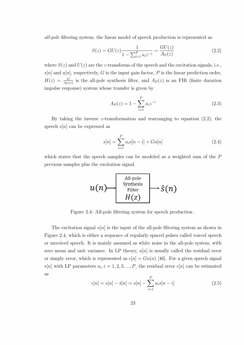
all-pole filtering system, the linear model of speech production is represented as

S(z) = GU(z)1

1−∑P

i=1 aiz−i

=GU(z)

AP (z)(2.2)

where S(z) and U(z) are the z-transforms of the speech and the excitation signals, i.e.,

s[n] and u[n], respectively, G is the input gain factor, P is the linear prediction order,

H(z) = GAP (z)

is the all-pole synthesis filter, and AP (z) is an FIR (finite duration

impulse response) system whose transfer is given by

AP (z) = 1−P∑

i=1

aiz−i (2.3)

By taking the inverse z-transformation and rearranging to equation (2.2), the

speech s[n] can be expressed as

s[n] =P∑

i=1

ais[n− i] +Gu[n] (2.4)

which states that the speech samples can be modeled as a weighted sum of the P

previous samples plus the excitation signal.

Figure 2.4: All-pole filtering system for speech production .

The excitation signal u[n] is the input of the all-pole filtering system as shown in

Figure 2.4, which is either a sequence of regularly spaced pulses called voiced speech

or unvoiced speech. It is mainly assumed as white noise in the all-pole system, with

zero mean and unit variance. In LP theory, u[n] is usually called the residual error

or simply error, which is represented as ε[n] = Gu(n) [46]. For a given speech signal

s[n] with LP parameters ai, i = 1, 2, 3, ..., P , the residual error ε[n] can be estimated

as

ε[n] = s[n]− s[n] = s[n]−P∑

i=1

ais[n− i] (2.5)

23

Figure 2.5: Estimation of residual error ε[n] using the prediction filter.

which is simply the output of the prediction filter excited by the speech samples s[n]

as shown in Figure 2.5.

The crucial task of LP modelling of speech is to accurately estimate the linear

prediction coefficients (LPCs). The next section describes the conventional LPC

estimation process in details.

2.2.1 Conventional LPC Estimation in Noise-free Case

In the conventional LPC estimation method, the analysis speech samples are consid-

ered as noise-free, that means it assumes the availability of the clean speech. There are

two methods for LPC estimation, i.e., autocorrelation and covariance based methods.

In this thesis, only the autocorrelation based technique is used in LPC estimation.

In general, the linear prediction coefficients ai’s are estimated by minimizing the

expectation of the residual energy ε2[n] or E[ε2[n]] as [46]

E[ε2[n]] = E[(s[n]−P∑

i=1

ais[n− i])2]

= E[s2[n]]− 2P∑

i=1

aiE[s[n]s[n− i]] +P∑

i=1

ai

P∑

j=1

ajE[s[n− i]s[n− j]]

= rss(0)− 2rTssA+A

TRssA (2.6)

where Rss = E[ssT ] is the autocorrelation matrix of the input vector sT = [s[n −

1], s[n − 2], . . . , s[n − P ]], rss = E[s[n]s] is the autocorrelation vector and AT =

[a1, a2, . . . , aP ] is the LPC vector.

From equation (2.6), the gradient of the mean square prediction error with respect

24

to the LPC vector A is given by

∂

∂AE[ε2[n]] = −2rT

ss+ 2AT

Rss (2.7)

where the gradient vector is defined as

∂

∂A= (

∂

∂a1,∂

∂a2, . . . ,

∂

∂aP)T (2.8)

The least mean square error solution is obtained by setting equation (2.7) to zero and

rearranging the terms, i.e.,

ATRss = r

Tss

(2.9)

Taking the transponse on both sides of equation (2.9), we get

(AT )TR

Tss

= (rT )T

ss(2.10)

We know that the transpose of a transpose matrix is the original matrix. Thus,

(AT )T= A and (rT )

T

ss= rss. Here, Rss is a symmetric metrix, and we know that

the transpose of a symmetric metrix is the matrix itself, i.e., RTss

= Rss. Therefore,

rearranging equation (2.10), we get

ARss = rss (2.11)

from which the linear prediction coefficient vector is solved as

A = R−1

ssrss (2.12)

or equivalently,

a1

a2

a3...

aP

=

rss(0) rss(1) rss(2) . . . rss(P − 1)

rss(1) rss(0) rss(1) . . . rss(P − 2)

rss(2) rss(1) rss(0) . . . rss(P − 3)...

.... . .

...

rss(P − 1) rss(P − 2) rss(P − 3) . . . rss(0)

−1

×

rss(1)

rss(2)

rss(3)...

rss(P )

(2.13)

The matrix Rss is called Toepiltz matrix which is symmetric with only P elements

provided that each diagonal element being identical. The Levinson-Durbin recursion

can be used to solve the matrix in order to get the linear prediction coefficients ai’s

25

[46]. In noise-free case, the LPC synthesis filter is stable, that means all the roots of

the denominator are inside the unit circle. Therefore, the estimated LPC coefficients

are accurate. However, in practice, we can access only the noisy speech. Therefore,

the next section describes the proposed LPC estimation method in noisy condition.

2.2.2 Existing LPC Estimation Methods in Noisy Conditions

The conventional LPC estimation technique requires that the spectral parameters

be estimated from the clean speech. This is because the LPCs are directly related

to the pole locations of the all-pole synthesis filter, which in principle are functions

of formant frequencies. When noise is introduced, however, the pole locations are

changed and the all-pole synthesis filter may no longer be stable, which leads to wrong

estimation of the LPCs. Moreover, the estimated LPCs contain severe temporal

variations as compared to those obtained from the clean speech. Therefore, these

coefficients may no longer represent the proper configurations and shapes of the glottal

source and the vocal tract system. On the other hand, the spectrum of the LPC

synthesis filter exhibits formant shifting and the bandwidth becomes wider, leading

to an overall degradation in the quality of the reconstructed speech. Therefore, it is

a very challenging task to estimate the LPC coefficients from the noisy speech.

To overcome this problem, numerous methods have been proposed in the last

few decades. However, obtaining a satisfactory solution preserving the stability of

the all-pole LPC synthesis filter, and providing an accurate estimation of the linear

prediction coefficients is still a challenging task. It is important to note that the

additive noise v(n) changes the speech generation process from AR model to an

auto regressive moving average (ARMA) process. Therefore, the LPC parameters

estimated from a noise corrupted speech using an all-pole synthesis filter become

biased, which is proportional to the inverse of the signal-to-noise ratio [47]. For noisy

speech y(n) = s(n) + v(n), where s(n) is the clean speech and v(n) is the zero mean

white noise, the biased autocorrelation function (ACF) is written as

Ryy(n) = Rss(n) + Rvv(n)

= Rss(n) + σ2vδ(n) (2.14)

where σ2v is the additive noise variance, Rvv(n) is the biased ACF of the additive noise

v(n), Ryy(n) and Rss(n) are the ACF of the noisy speech y(n) and that of the clean

26

speech s(n), respectively.

The main idea here is to subtract the noise power from the ACF of the noisy speech

Ryy(n) at zero lag, n = 0. To do this, an iterative noise subtraction based method

for the LPC estimation has been introduced in [48], where noise compensation is

achieved by gradually subtracting a noise power estimated from the ACF of the noisy

speech. The main drawback of this method is that it assumes the noise variance to be

known. Instead of deriving the exact noise variance, the adaptive method proposed

in [49] determines a suitable bias that should be subtracted from the zero-lag of the

ACF of the noisy speech. In this method, the stability of the all-pole LPC synthesis

filter is ensured when the noise variance is less than the minimum eigenvalue of the

autocorrelation matrix. In [47], the noise periodogram is obtained first by applying a

simplified noise PSD estimator on the calculated noisy periodogram. Then, the effect

of noise on the spectral parameters is decreased by gradually subtracting values of the

resulting noise autocorrelation coefficients from the coefficients derived from the noisy

speech. The LPCs are estimated from the absolute value of the estimated coefficients.

This method ensures a significant decrease in the degrading effect of noise while the

estimated LPCs are more accurate. Higher order Yule-Walker equation has been used

in [50], where Rss(0) is not involved in the evaluation of Rss(n) from the noisy speech

y(n) for all lags other than zero. This method was developed only for estimating

the LPCs from the white noise corrupted speech and under the assumption that the

noise variance is known. Another shortcoming of this method is that the energy of

the additive noise spreads all over the autocorrelation lags of the analysis speech,

which may lead to a substantial increase in the variance of the estimated spectral

parameters.

2.3 Conventional Kalman Filter for Speech En-

hancement

The theory of Kalman filter is established on state-space model where a state equation

models the dynamics of a signal generation process, an observation equation, on the

other hand, models the noisy and distorted nature of the signal. The linear prediction

coefficients and additive noise variance are two important state-space model parame-

ters for KF implementation. The operation principle of the KF includes a prediction

27

step and a correction step. In the prediction step, it estimates the a posteriori error

covariance by using the previous samples of the state-space model. The KF basi-

cally reduces the additive noise effect by minimizing the a posteriori error covariance

achieved at each step through recursive procedures. To do this, in the correction step,

the a posteriori error covariance is processed recursively until its minimization. The

overall operation is performed on a frame-by-frame basis. In this way, at the end of

the recursive procedure, the additive noise is statistically minimized [51].

The clean speech s(n) is modeled as a P th order auto-regressive (AR) process as

given by

s(n) =

p∑

i=1

ais(n− i) + u(n) (2.15)

and the noisy speech is defined as

y(n) = s(n) + v(n) (2.16)

where s(n) is the nth sample of the clean speech, y(n) is the nth sample of the noisy

observation, ai is the ith LPC coefficient, u(n) and v(n) are uncorrelated Gaussian

white noise sequences with zero mean and the variances σ2u and σ2

v , respectively.

This system can be represented by the following state-space model (SSM), where

the bold faced letters represent vectors or matrices

State Equation:

x(n) = Φx(n− 1) +Gu(n) (2.17)

Observation Equation:

y(n) = Hx(n) + v(n) (2.18)

In the above SSM,

1. x(n) is a P -dimensional signal vector, or the state parameter vector at time n

which can be expressed as

x(n) = [s(n− p+ 1) s(n− p+ 2) . . . s(n)]T (2.19)

2. Φ is a P × P -dimensional state transition matrix that relates the states of the

28

process at times n− 1 and n which can be written as

Φ =

0 1 0 . . . 0

0 0 1 . . . 0...

......

. . ....

0 0 0 . . . 1

ap ap−1 ap−2 . . . a1

,

3. G and H are the P × 1 input vector and the 1 × P observation row vector,

respectively, which can be represented as

H = GT =

[

0 0 0 . . . 1]

,

4. y(n) is the observation measurement of the SSM at time n.

If x(n) and y(n) are assumed to be jointly Gaussian, the Kalman filter gives an

optimal estimate of the x(n) given the noisy data y(n), y(n− 1), ...., y(1). For such

a Gaussian distribution, the optimal estimate is called the minimum mean squared

error (MMSE) estimate as given by

x(n|n) = E[x(n)|y(n), y(n− 1), ...., y(1)] (2.20)

The corresponding a posteriori estimation error covariance Σx(n|n) is then defined

as

Σx(n|n) = E[ε(n|n)εT (n|n)] (2.21)

where ε(n|n) is the a posteriori estimation error which is defined as

ε(n|n) = x(n|n)− x(n|n) (2.22)

Similarly, the one step prediction error also called the a priori estimation error ε(n|n−

1) of x(n|n) and the associated a priori error covariance matrix Σx(n|n − 1) are

defined as

ε(n|n− 1) = x(n|n)− x(n|n− 1) (2.23)

Σx(n|n− 1) = E[ε(n|n− 1)εT (n|n− 1)] (2.24)

The goal here is to find an equation that computes an a posteriori state estimate

as a linear combination of an a priori estimate (also called prediction) and a weighted

29

difference between the actual measurement and the one-step measurement prediction

[51]. More specifically, it is possible to write an update equation for the new estimate

x(n|n) by combing the old estimate x(n|n− 1) with the measurement prediction as

x(n|n) = x(n|n− 1) +K(n)[y(n)−Hx(n|n− 1)] (2.25)

where y(n)−Hx(n|n− 1) is called the measurement innovation, which is defined as

e(n) = y(n)−Hx(n|n− 1) (2.26)

The measurement innovation reflects the discrepancy between the predicted measure-

ment Hx(n|n−1) and the actual measurement y(n). The innovation e(n) is a special

stochastic process that plays a central role in the development of the Kalman filter

theory [51, 52]. The P × P matrix, K(n) in equation (2.25) is called Kalman gain

which also plays a very important role. The Kalman gain vector K(n) should be

determined such that the a posteriori error covariance is minimized. Substitution of

equation (2.18) into (2.25) gives

x(n|n) = x(n|n− 1) +K(n)[Hx(n) + v(n)−Hx(n|n− 1)] (2.27)

By substituting equation (2.27) into (2.21) and rearranging the terms, we get

Σx(n|n) = E[[(I−K(n)H)ε(n|n−1)−K(n)v(n)][(I−K(n)H)ε(n|n−1)−K(n)v(n)]T ]

(2.28)

where ε(n|n− 1) is the error of the a prior estimate, which is uncorrelated with the

measurement noise v(n). Therefore, equation (2.28) is re-written as

Σx(n|n) = [I−K(n)H ]E[ε(n|n−1)εT (n|n−1)][I−K(n)H ]T+K(n)E[v(n)vT (n)]KT (n)

(2.29)

Considering σ2v = E[v(n)vT (n)] and using equation (2.24) into (2.29) gives

Σx(n|n) = [I −K(n)H ]Σx(n|n− 1)[I −K(n)H ]T +K(n)σ2vK

T (n) (2.30)

Equation (2.30) is the error covariance update equation where Σx(n|n − 1) is the

prior estimate of Σx(n|n).

The diagonal elements of the covariance matrix Σx(n|n) contain the mean squared

error (MSE). We know that the sum of the diagonal elements of a matrix is the trace

30

of that matrix. Therefore, the MSE may be minimized by minimizing the trace of

Σx(n|n). Rewriting equation (2.30) as

Σx(n|n) = Σx(n|n− 1)−K(n)HΣx(n|n− 1)−Σx(n|n− 1)HTK

T (n)

+K(n)[HΣx(n|n− 1)HT + σ2v ]K

T (n) (2.31)

and taking the trace on both sides of (2.31) rearranging the terms, we get

Tr[Σx(n|n)] = Tr[Σx(n|n− 1)]− 2Tr[K(n)HΣx(n|n− 1)]

+ Tr[K(n)(HΣx(n|n− 1)HT + σ2v)K

T (n)] (2.32)

Taking the partial derivative on both sides of the equation (2.32) with respect to

K(n) gives

dTr[Σx(n|n)]

dK(n)= −2[HΣx(n|n− 1)]T + 2K(n)[HΣx(n|n− 1)HT + σ2

v ] (2.33)

from which K(n) can be computed by setting the left side of (2.33) to zero as

K(n) = Σx(n|n− 1)HT [HΣx(n|n− 1)HT + σ2v ]

−1 (2.34)

Using the equations (2.34), (2.25), and (2.26), the update equation of the current

state x(n|n) is given by

x(n|n) = x(n|n− 1) +K(n)e(n) (2.35)

The update equation for the error covariance matrix with optimal gain is obtained

through the substitution of equation (2.34) into (2.31), namely,

Σx(n|n) = Σx(n|n− 1)−K(n)HΣx(n|n− 1)

= (I −K(n)H)Σx(n|n− 1) (2.36)

Finally, the enhanced speech sample s(n) at time n is given by

s(n) = Hx(n|n) (2.37)

The above KF based speech enhancement algorithm is summarized below

31

Initialization:

x(0|0) = 0 (2.38)

Σx(0|0) = [0]p×p (2.39)

Time update (predictor):

x(n|n− 1) = Φx(n− 1|n− 1) (2.40)

Σx(n|n− 1) = ΦΣx(n− 1|n− 1)ΦT +Gσ2uG

T (2.41)

Measurement update (corrector):

e(n) = y(n)−Hx(n|n− 1) (2.42)

K(n) = Σx(n|n− 1)HT (HΣx(n|n− 1)HT + σ2v)

−1 (2.43)

x(n|n) = x(n|n− 1) +K(n)e(n) (2.44)

Σx(n|n) = (I −K(n)H)Σx(n|n− 1) (2.45)

Estimated speech (at time n):

s(n) = Hx(n|n) (2.46)

The above procedures are repeated for the following speech frames and continued

until the end of all frames to be processed. At the end of processing all noisy speech

frames, the ultimate enhanced speech s(n) is obtained. The next section gives the

proposed speech enhancement based on non-iterative Kalman filter.

2.4 Proposed Non-Iterative Kalman Filter based

Speech Enhancement

In this section, we propose a non-iterative Kalman filter for speech enhancement, in

which the state-space model parameters, namely, LPC and noise variance, are esti-

mated from the noisy speech. The new method is not limited to reduce only the white

Gaussian noise, rather it is expected to reduce the different environmental noises. For

LPC estimation, a combined speech smoothing and autocorrelation method is pro-

posed. A new method based on a lower-order truncated Taylor series approximation

of the noisy speech along with a difference operation serving as high-pass filtering is

32

also introduced for the noise variance estimation. The Kalman filter is then developed

with these estimated parameters.

It is noted that the P × P dimensional Kalman gain function K(n) (2.34) has

been used in the conventional Kalman filter. The update equation (2.35) indicates

that the a priori estimate x(n|n − 1) is a P × 1 dimensional matrix which is added

with K(n)e(n) that should also be P × 1 dimensional according to the linear algebra

operation. Therefore, in the proposed non-iterative Kalman filter, the modified P ×1

dimensional K(n) is obtained as

K(n) = [Σx(n|n− 1)HT (HΣx(n|n− 1)HT + σ2v)

−1]HT (2.47)

The proposed algorithm works on a frame-by-frame basis, each frame containing

N speech samples. The proposed non-iterative KF based speech enhancement is sum-

marized as follows

Initialization:

x(0|0) = 0 (2.48)

Σx(0|0) = [0]p×p (2.49)

Φ =

0 1 0 . . . 0

0 0 1 . . . 0...

......

. . ....

0 0 0 . . . 1

ap ap−1 ap−2 . . . a1

(2.50)

For n = 1 to N do

Time update (predictor):

x(n|n− 1) = Φx(n− 1|n− 1) (2.51)

Σx(n|n− 1) = ΦΣx(n− 1|n− 1)ΦT +Gσ2uG

T (2.52)

33

Measurement update (corrector):

e(n) = y(n)−Hx(n|n− 1) (2.53)

K(n) = [Σx(n|n− 1)HT (HΣx(n|n− 1)HT + σ2v)

−1]HT (2.54)

x(n|n) = x(n|n− 1) +K(n)e(n) (2.55)

Σx(n|n) = (I −K(n)H)Σx(n|n− 1) (2.56)

Estimated speech (at time n):

s(n) = Hx(n|n) (2.57)

End for

The above procedure is repeated for the following frames and continued until the

end of the last noisy frame, yielding the ultimate enhanced speech s(n).

2.4.1 Proposed Noise Variance Estimation Algorithm

The noise variance σ2v is estimated using a new method proposed based on a lower-

order truncated approximation of Taylor series. The clean speech samples given

in equation (1.1) can be well approximated locally at any point on a curve by a

lower order polynomial, which can be thought of as a truncated local Taylor series

approximation. The main idea here is to apply a low-order difference operation, which

is simply an approximation to a certain order differentiation of the truncated series

so that the lower order terms are eliminated, while leaving behind only a high-order

terms, mainly composed of high-frequency noise components, from which the noise

variance is estimated. The differentiation can be represented mathematically as a

convolution of the noisy observation with an FIR (finite-duration impulse response)

template as shown in Table 1 [53].

Table 1: Derivative Templates.

Template (w) Differentiation Order

[-1 1] First Derivative[1 -2 1] Second Derivative

[1 -3 3 -1] Third Derivative[1 -4 6 -4 1] Forth Derivative

34

noises, respectively (input SNR=0dB). From Figure 2.6, it is observed the estimated

noise variance is very close to the original noise variance, even at 0dB input SNR.

2.4.2 Proposed LPC Estimation Algorithm

Here, we propose an LPC estimation algorithm based on speech smoothing and auto-

correlation. First, the smoothing is used as a pre-processing of the noisy speech y(n)

which can remove some unwanted high-frequency noise components in advance. The

simplest smoothing can be done with a simple rectangular window serving as an FIR

filter. For example, a 3-point smooth (i.e., the window width is m = 3) at sample

point n is represented as

y(n) =y(n− 1) + y(n) + y(n+ 1)

3(2.60)

where y(n) is the nth sample of the smoothed speech.

There are many different smoothing kernels or windows available, such as, trian-

gular, rectangular, Hamming window, etc. [53]. However, the choice of the smoothing

kernel depends on the domain of processing as well as applications to be considered.

The following table shows some smoothing kernels used in most applications.

Table 2: Different Smoothing Kernels

Smoothing Kernel (w) Kernel Name

[1 1 1] 3-point boxcar (sliding average)

[1 1 1 1 1] 5-point boxcar (sliding average)

[1 2 1] 3-point triangular window

[1 2 3 2 1] 5 point triangular window

The width of the smoothing kernel m is usually chosen to be an odd integer, so

that the smooth coefficients are symmetrically balanced around the central point.

In the proposed LPC estimation algorithm, the smoothing is performed with a 5-

point rectangular kernel w = [1 1 1 1 1] for the sample points n = 3 to N − 2,

where N is the number of sample points in each analysis speech frame. Here, the

rectangular kernel is used since it is fitted well in time-domain rather than other

smoothing kernels. It is observed that the smoothing operation cannot be performed

for the first two points or for the last two points within each frame. In general, for

36

an m-width smoothing kernel, there will be (m − 1)/2 points at the beginning, and

(m − 1)/2 points at the end of the analysis speech for which a complete m-width

smooth cannot be calculated like the other points. This phenomenon is called the

edge effects and the lost points problem. In order to address this issue, (m − 1)/2

points zero padding is done at the beginning and the end of the analysis speech frame.

Figure 2.7: (a) clean speech (male) frame, (b) white noise (input SNR=5dB) cor-

rupted frame, and is the corresponding smoothed speech frame.

Figure 2.8: (a) clean speech (female) frame, (b) non-stationary noise (input

SNR=5dB) corrupted frame, and is the corresponding smoothed speech frame.

The underlying principal is to perform smoothing on a sample-by-sample basis

within each analysis speech frame. The general smoothing operation can be repre-

sented mathematically using the convolution operation between the noisy speech y(n)

37

and the smoothing kernel w as

y(n) =1

m

m−1∑

i=0

w(i)y[n− (m− 1)/2 + i] (2.61)

It is noted that the convolution equation (2.61) is modified slightly as compared

to the conventional convolution so that the smooth coefficients are symmetrically

balanced around the central point. Figure 2.7 and 2.8 show the effect of smoothing

process, where the clean speech is corrupted by the white and non-stationary noises

(input SNR=5dB).

The smoothing can never reduce the additive noise effects completely, since the

noise components are spreaded out over a wide range of frequencies, and smooth-

ing simply reduces the noise in part of its frequency range. Although it can remove

some high-frequency noise components, it underestimates the contribution of the low-

frequency noise components, which is hard to estimate visually because there are so

few low-frequency components in the noisy speech. This remaining low-frequency

noise components can affect the LPC estimation accuracy of the autocorralation

method. In order to remove such noise components effectively, the estimated noise

variance σ2v in (2.59) is subtracted from the zero-lag of Ryy(n) in (2.62), where Ryy(n)

is the ACF of y(n). Generalizing the result given in equation (2.14), the noiseless

Rss(n) is estimated as

Rss(n) =

Ryy(n)− σ2vδ(n), n = 0

Ryy(n), otherwise(2.62)

where

Ryy(n) =N−1+P∑

i=0

y[i]y[n− i] (2.63)

and y(n) is the smoothed speech samples, σ2v is the estimated noise variance obtained

from equation (2.59). Using the same procedure of the equation (2.13), the estimated

ACFs Rss(n) can be represented in matrix notation as

a1

a2...

aP

=

Rss(0) Rss(1) . . . Rss(P − 1)

Rss(1) Rss(0) . . . Rss(P − 2)...

.... . .

...

Rss(P − 1) Rss(P − 2) . . . Rss(0)

−1

×

Rss(1)

Rss(2)...

Rss(P )

(2.64)

38

By solving equation (2.64) using the Levinson-Durbin recursion, the LPC coeffi-

cients ai’s are estimated [45, 49] effectively.

It is important to understand the link between the spectrum of a speech and its

prediction coefficients. To do this, using equation (2.2) and (2.3) and setting z = ejω,

the spectrum of speech s[n] is represented as

S(ejω) =G2|U(ejω)|2

|1−∑P

i=1 aie−jwi|2

(2.65)

It is noted that U(ejω) is termed as the prediction error in the linear prediction theory

which is assumed to be white Gaussian noise with zero mean and unit variance.

Therefore, its magnitude spectrum is assumed to be constant, i.e., |U(ejω)| = 1 for

all ω [46]. Then equation (2.65) reduces to

S(ejω) =G2

|1−∑P

i=1 aie−jwi|2

(2.66)

Therefore, the spectrum of a speech signal can be modeled by the frequency re-

sponse of an all-pole filter, whose parameters are the linear prediction coefficients

[46]. Figure 2.9 shows the spectra of the clean, the degraded, and the estimated

speech corresponding to the frequency response of an all-pole filter in the presence

of non-stationary noise (SNR=0dB), where the LPCs are obtained from these speech

samples separately. It is observed that the estimated spectra (solid line) is closer

to the clean speech spectra (dashed line). In particular, the shape of the first two

formants is better preserved in the estimated spectra as compared to the clean speech

spectra (dashed line). From Figure 2.10, it is also observed that the estimated spectra

(solid line) is a close approximation to the clean speech spectra (dashed line) in the

presence of pink noise.

2.5 Proposed Speech Enhancement Algorithm us-

ing Iterative Kalman Filter

In the non-iterative KF method proposed in the previous section, the model parame-

ters are estimated in non ideal case. Although it performs relatively well in different

noisy conditions, yet it has some limitations, especially at low SNRs where the ac-

curacy of the estimated LPC decreases. The possible phenomenon of this effect may

introduce some musical noise as well as distortion in the enhanced speech.

39

Figure 2.9: Power spectra comparison between the clean speech (dashed), degradedspeech (dotted), and estimated speech (solid), in the presence of non-stationary noise(Input SNR= 0dB).

Figure 2.10: Power spectra comparison between the clean speech (dashed), degradedspeech (dotted), and estimated speech (solid), in the presence of pink noise (InputSNR = 0dB).

40

In order to enhance the SE performance as well as parameter estimation accuracy

in noisy conditions, an iterative Kalman filter based SE method is presented in this

section, which also operates on a frame-by-frame basis but contains two loops of

iterations, called inner and outer loops for each frame. In the inner loop, the state-

space model parameters of the KF are updated sample-by-sample through an iterative

procedure. The additive noise components are reduced significantly when the inner

loop is completed for one entire frame. Then, the LPCs and other state-space model

parameters are re-estimated from the same processed speech frame for the 2nd inner

loop iteration. The outer loop iterative procedure stops when the KF converges or

the preset maximum number of iterations is exhausted, giving the further enhanced

result of the same speech frame to the input noisy speech frame. The same procedure

will repeat for the following frames until the end of all analysis speech frames being

processed.

For each frame of N samples, we set D as the maximum number of iterations.

The proposed iterative KF based speech enhancement can be summarized below.

Estimate LPCs from y(n), yielding ak, k = 1, 2, 3, . . . , P . Let s(0)(n) = y(n), n =

1, 2, 3, . . . , N .

For j = 1 to D do [outer loop]

Initialization:

x(j)(0|0) = 0 (2.67)

Σx(j)(0|0) = [0]p×p (2.68)

Φ(j) =

0 1 0 . . . 0

0 0 1 . . . 0...

......

. . ....

0 0 0 . . . 1

ap ap−1 ap−2 . . . a1

(2.69)

For n = 1 to N do [inner loop]

Time update (predictor):

x(j)(n|n− 1) = Φ(j)

x(j)(n− 1|n− 1) (2.70)

Σx(j)(n|n− 1) = Φ(j)Σx

(j)(n− 1|n− 1)Φ(j)T +HTσ2

uH (2.71)

41

Measurement update (corrector):

e(j)(n) = s(j−1)(n)−Hx(j)(n|n− 1) (2.72)

K(j)(n) = [Σx

(j)(n|n)HT (HΣx(j)(n|n)HT

+ σ2v)

−1]HT (2.73)

x(j)(n|n) = x

(j)(n|n− 1) +K(j)(n)e(j)(n) (2.74)

Σx(j)(n|n) = (I −K

(j)(n)H)Σx(j)(n|n− 1) (2.75)

Estimate enhanced speech (at time n):

s(j)(n) = Hx(j)(n|n) (2.76)

End for [inner loop]

If |1− k(j)1 ||aP | < 1 (where k

(j)1 is the 1st element of K(j)(n)) [KF Converges]

Output the enhanced speech s(n) and stop.

End for [outer loop]

Else

Re-estimate LPCs ak(k = 1, 2, 3, . . . , P ) from the jth processed frame s(j)(n).

Repeat for [outer loop]

The above procedure is repeated for the following frames and continued until the

end of the last frame, resulting in ultimate enhanced speech s(n).

42

Figure 2.11: Power spectra comparison between the clean speech (magenta), degraded

speech (red), estimated(NIT-KF) (black), and estimated(IT-KF) (blue) in presence

of the non-stationary noise (Input SNR = 0dB).

Figure 2.12: Power spectra comparison between the clean speech (magenta), degraded

speech (red), estimated(NIT-KF) (black), and estimated(IT-KF) (blue) in the pres-

ence of the pink noise (Input SNR = 0dB).

43

In this proposed method, the LPCs are re-estimated for several times using the

enhanced speech frame resulting from the inner iteration of the Kalman filter. Fig-

ures 2.11 and 2.12 compare the estimated speech spectra used in the non-iterative

(NIT-KF), and iterative (IT-KF) Kalman filter based methods with the clean speech

and the degraded speech spectra in the presence of non-stationary and pink noises,

respectively with input SNR=0dB.

From Figure 2.11, it is observed that the estimated speech spectra obtained from

the enhanced speech frame provided by the iterative Kalman filter estimated(IT-

KF) (blue) is closer to the clean speech spectra (magenta) than the estimated spectra

(black) obtained from the non-iterative Kalman filter estimated(NIT-KF) method. In

particular, the shapes of all the four formants are better preserved in the estimated(IT-

KF) (blue) as compared to the clean speech spectra (magenta). From Figure 2.26, it

is also observed that the estimated(IT-KF) (blue) is also closer to the clean speech

spectra (magenta) in the presence of pink noise. In the overall comparison, it is clearly

observed that the estimated(IT-KF) (blue) can preserve all the formant frequencies

effectively, while the estimated(NIT-KF) (black) sometimes fails as compared to the

clean speech spectra (magenta).

2.6 Performance Comparisons of the Proposed Meth-

ods

To evaluate the performance of the proposed methods, we use the NOIZEUS speech

corpus database, which is composed of 30 phonetically balanced sentences belonging

to six speakers [1]. The speech is sampled at 16 kHz and corrupted by white Gaussian,

babble and car noises taken from the Noisex-92 database [54] for a wide range of input

SNR (-10dB to 15dB). The LPC order considered in this simulation is P = 8. The

criteria used for the performance evaluation is the perceptual evaluation of speech

quality (PESQ) [55]. PESQ takes values between 1 (worse) and 4.5 (best). The

detailed description of PESQ will be discussed in chapter 4.

The performances of the proposed methods based on the non-iterative Kalman

filter (Proposed-NIT-KF), iterative Kalman filter (Proposed-IT-KF) are evaluated

and compared with some existing methods, namely, LPCs enhancement in iterative

Kalman filtering (LPC-IT-KF) [26] and fast converging iterative Kalman filtering

44

based method (FC-IT-KF) [25].

Figure 2.13 shows the performance comparison between the proposed methods

and other existing methods in terms of PESQ for the white, babble and car noise

experiments. From Figure 2.13, it is observed that the proposed method performs

much better than the existing methods consistently even at low SNRs in all three

noises. This is attributed to the good overall reduction of the background noise,

residual noise and distortion.

Figure 2.13: Performance comparison between the proposed methods and other ex-isting competitive methods in terms of PESQ. The speech utterances are corruptedby (a): White, (b): Babble and (c): Car noises for a wide range of input SNRs(-10dBto 15dB).

Other extensive simulation results for the proposed methods in the presence of

other environmental noises will be shown and discussed in Chapter 4.

2.7 Conclusion

In this chapter, at first, some background material including human speech modeling

using LPC analysis, conventional LPC estimation in noise-free and noisy conditions,

conventional KF for speech enhancement has been introduced. In the conventional

KF, the state-space model parameters, namely, LPC and noise variance are estimated

from the clean speech and noisy speech, respectively, which is impractical. In order to

45

overcome these limitations, we proposed a non-iterative Kalman filter based speech

enhancement approach, where the LPC and noise variance are estimated from noisy

speech. In addition, for LPC estimation in noisy conditions, a smoothing and au-

tocorrelation based combined method has been proposed. A new method based on

lower-order truncated approximation of Taylor series along with a difference opera-

tion serving as high-pass filtering, for the estimation of the noise variance was also

proposed. Moreover, the proposed parameter estimation methods perform well in

different environmental noises, which compactly make the non-iterative Kalman filter

to reduce the environmental noises. Some existing Kalman filter based methods, on

the other hand, are limited to reduce only white noise as mentined in the literature

[13].

The non-iterative Kalman filter, however, introduce some musical noise and dis-

tortion in the enhanced speech. In order to improve the speech enhancement accuracy

as well as parameter estimation in noisy conditions, an iterative Kalman filter based

speech enhancement method has been proposed as the second approach, where the

state-spate model parameters of the Kalman filter have been estimated through a

two-loop iteration process. It is important to note that the LPC coefficients have

been updated based on the partially enhanced speech in each frame for a better ac-

curacy, thus making the iterative Kalman filter method better than the non-iterative

Kalman filter. Specifically, unlike the besic version of Kalman filter, which is to re-

duce only white noise, the iterative version of Kalman filter was proposed for colored

noise corrupted speech enhancement. In addition, it can update better Kalman filter

parameters through iterations as well as improve speech enhancement performance

over the non-iterative Kalman filter.

Through simulation studies, we have found that the proposed methods are capable

of reducing the adverse environmental noises significantly for a wide range of input

SNRs, and outperform several existing methods in the literature.

46

Chapter 3

Proposed Speech Enhacement

Algorithm using Sub-band

Iterative Kalman Filter

3.1 Introduction

The iterative Kalman filter based speech enhancement presented in chapter 2 per-

forms better than existing Kalman filter based methods. This is because it can

reduce the residual noise in the enhanced speech by employing better Kalman filter

parameters through iterations. However, some musical-like artifacts still remain in

the enhanced speech. Moreover, the enhanced speech also suffers from a little bit

distortion, which can degrade the quality of the enhanced speech. In order to further

improve the speech quality, a sub-band iterative Kalman filter based speech enhance-

ment algorithm is proposed in this chapter, where a wavelet filter-bank is used to

decompose the noisy speech into a set of sub-bands prior to Kalman filtering. It

is important to note that the decomposed sub-bands contain some hidden informa-

tion that may not be available in the full-band noisy speech. As such, in the new

method, the state-space model parameters of the Kalman filter, namely, the LPCs

and the excitation noise variance, are estimated from the sub-band speech rather than

the full-band noisy speech as done in the previous two approaches. The estimated

model parameters have better accuracy than those estimated from the full-band noisy

speech, leading to a better performance of the sub-band iterative Kalman filter based

47

speech enhancement algorithm. The following sections first introduce the wavelet

and filter-bank fundamentals, and then present the sub-band iterative Kalman fil-

ter based approach, including the parameter estimation from the sub-bands of noisy

speech. Finally, simulation results will be provided to show the performance of the

proposed sub-band Kalman filter based method followed by concluding remarks.

3.2 Wavelets and Filter-bank

The wavelet filter-bank in general is an array of band-pass filters that separates the

input signal into multiple components, where each one carrying a single frequency sub-

band of the original signal [56]. The generated sub-bands contain further details or

other hidden information of the analysis signal that may not readily be available in the

full-band signal yet could be exploited by processing each sub-band separately. The

decomposition process performed by the wavelet filter-bank is called analysis process

and the output of each analysis process is referred to as a sub-band signal. The

reconstruction process is called synthesis process, which is to reconstruct the original

complete signal from sub-band signals. The main requirement for wavelet filter-bank

design is to meet the perfect reconstruction (PR) criterion which intuitively means

that the signal does not get corrupted by the filter-bank. Moreover, in a PR system,

there is no error at the output, meaning that the output is simply a time-delayed

copy of the input signal [57].

Multirate filter-banks are the general building blocks for sub-band decomposition.

Figure 3.1 shows anM -channel filter-bank structure where Hi(z)’s and Gi(z)’s are the

analysis and synthesis filters respectively. The characteristics of these filters depend

on the application to be used and the dimensionality of the problem. The multi-

layered wavelet filter-bank structure shown in Figure 3.1 decomposes the input signal

into a series of different frequency space, called the multi-resolution analysis of a

signal in different scales which can demonstrate different frequency characteristics of

a signal. More specifically, a two-channel filter-bank decomposes the analysis signal

into two parts, one is detail part and the other is approximation part. The detail

part contains the high-frequency information of the signal, and the approximation

part, on the other hand, contains the low-frequency information of the signal. A

multi-channel filter-bank can be implemented by performing a series of two-channel

48

(a)

(b)

Figure 3.1: (a) Block diagram of an M -channel filter-bank structure, and (b) approx-imate frequency responses of analysis filters.

decomposition, where the approximation or detail part can be further decomposed

again in order to obtain further detail and approximation part in a higher scale.

The level of decomposition for extracting the essential information from the sub-

band signals depends on the applications. Also, the multiple band decomposition

may be obtained by simultaneously applying an M -channel filter-bank directly [58].

In general, the sub-band decomposition should be properly carried out such that it

provides the following advantages.

• Give sufficient information for both analysis and synthesis procedures.

• Reduce the computational time sufficiently.

• It is relatively easier to implement.

• It can analyze the signal at different frequency bands with different resolutions.

• It decomposes the signal into a coarse approximation and detail information.

Using the advantages of the sub-band decomposition, many speech enhancement

algorithms have been introduced in the literature. Most of these algorithms combine

49

wavelet filter-bank with other methods in order to improve the performance of the

speech enhancement. Here, we mainly focus on the wavelet sub-band decomposition

process, and consider both the two-channel and multi-channel decomposition cases.

3.2.1 Two-channel Filter-bank Structure

A 2-channel filter-bank is shown in Figure 3.2,

(a)

(b)

Figure 3.2: (a) Block diagram of a simple two-channel filter-bank structure, and (b)approximate frequency responses of analysis filters.

where a discrete time signal y(n) enters the analysis bank composed of filters

H0(z) and H1(z) which separate the frequency content of the input signal in frequency

bands of equal width. Further, H0(z) and H1(z) are a low-pass and a high-pass filters,

respectively. The output of each filter contains half-band the frequency content of

the original signal y(n), with an equal sampling rate [57]. The two outputs together

contain the same frequency content as the original signal y(n), but the amount of

data is doubled. Therefore, downsampling by a factor two, denoted by ↓ 2, is applied

to the outputs of the filters in the analysis bank. Reconstruction of the original

signal is possible using the synthesis filter bank and the rate-reduced two-channel

signals [59]. In the synthesis bank, the signals are upsampled by ↑ 2 and passed

through the synthesis filters G0(z) and G1(z) respectively. The filters in the synthesis

bank provide the same characteristics as compared to the filters in the analysis bank.

50

Finally, the reconstructed signal y(n) is obtained by summing up the outputs of

the filters in the synthesis filter-bank. The output signals, c1(n), and c2(n) of the

analysis filter-bank are called the sub-bands. It is important to note that the efficient

use of the up-sampling and down-sampling in the analysis and synthesis bank does

not guarantee the exact reconstruction of the original input signal y(n). In order to

design a practical filter-bank, PR condition of the filter-bank have to be met [60],

which is described in the next subsection.

3.2.2 Perfect Reconstruction of Two-channel Filter-bank

Figure 3.2 is used here as an example to drive the PR conditions. Consider N0 and N1

be the length of the low-pass and high-pass filters H0(z) and H1(z), respectively in the

analysis bank as shown in Figure 3.2. Then the input-output relation is represented

as

Y (z) = T0(z)Y (z) + T1(z)Y (−z) (3.1)

where T0(z) and T1(z) are given by

T0(z) =1

2[G0(z)H0(z) +G1(z)H1(z)] (3.2)

T1(z) =1

2[G0(z)H0(−z) +G1(z)H1(−z)] (3.3)

The transfer functions T0(z) and T1(z) are called the distortion and aliasing trans-

fer functions of the system. In order to design a PR filter-bank, it is necessary to find

Hk(z) and Gk(z) such that the output is a delayed copy of the input. That means,

the filters have to satisfy the following two conditions

G0(z)H0(z) +G1(z)H1(z) = z−n0 (3.4)

G0(z)H0(−z) +G1(z)H1(−z) = 0 (3.5)

where n0 indicates a time delay and equation (3.5) indicates the aliasing free condi-

tions, which can be satisfied by choosing

G0(z) = H1(−z), and G1(z) = −H0(−z) (3.6)

The above condition implies that in the synthesis bank, the impulse response of the

low-pass filter g0[n] is obtained by altering the sign of the impulse response of the

high-pass filter h1[n], i.e.;

g0[n] = (−1)nh1[n] (3.7)

51

and similarly we have

g1[n] = (−1)n+1h0[n] (3.8)

where h0[n] and h1[n] are the impulse responses of the low-pass and high-pass filters

in the analysis bank while g0[n] and g1[n] are the low-pass and high-pass filters in the

synthesis bank.

If equations (3.4) and (3.5) are satisfied, the output of the two-channel filter-bank

in Figure 3.2 is a delayed version of the input signal, i.e.;

Y (z) = z−n0Y (z) (3.9)

Rearranging equation (3.6) yields

H1(z) = G0(−z), and G1(z) = −H0(−z) (3.10)

Submitting the equation (3.10) into (3.4) gives

H0(z)G0(z)−H0(−z)G0(−z) = P0(z)− P0(−z) = z−n0 (3.11)

where P0(z) denotes the product of the two low-pass filters, H0(z) and G0(z), namely,

P0(z) = H0(z)G0(z) (3.12)

Equation (3.11) indicates that the product of all the odd terms of the two low-pass

filters, H0(z) and G0(z) must be zero, except for order n0 where the even order terms

are arbitrary. The delay parameter n0 must be odd which is usually the center of the

filter P0(z). These observations indicate that the coefficients of P0(z) can be written

as

p0[n] =

0, if n is odd and n 6= n0

1, if n = n0

arbitary, if n is even

(3.13)

Consequently, the two-channel PR filter-bank design reduces to two steps

1. Design a filter P0(z) that satisfies equation (3.13).

2. Factorize P0(z) into H0(z) and G0(z), then use equation (3.10) to compute

H1(z) and G1(z) respectively.

52

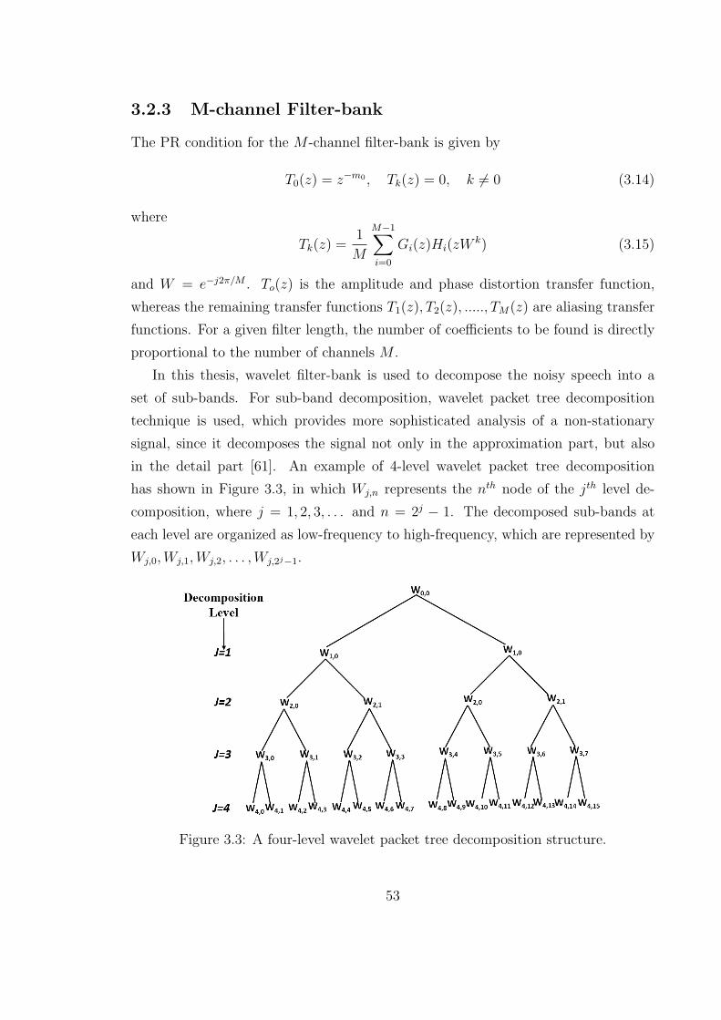
3.2.3 M-channel Filter-bank

The PR condition for the M -channel filter-bank is given by

T0(z) = z−m0 , Tk(z) = 0, k 6= 0 (3.14)

where

Tk(z) =1

M

M−1∑

i=0

Gi(z)Hi(zWk) (3.15)

and W = e−j2π/M . To(z) is the amplitude and phase distortion transfer function,

whereas the remaining transfer functions T1(z), T2(z), ....., TM(z) are aliasing transfer

functions. For a given filter length, the number of coefficients to be found is directly

proportional to the number of channels M .

In this thesis, wavelet filter-bank is used to decompose the noisy speech into a

set of sub-bands. For sub-band decomposition, wavelet packet tree decomposition

technique is used, which provides more sophisticated analysis of a non-stationary

signal, since it decomposes the signal not only in the approximation part, but also

in the detail part [61]. An example of 4-level wavelet packet tree decomposition

has shown in Figure 3.3, in which Wj,n represents the nth node of the jth level de-

composition, where j = 1, 2, 3, . . . and n = 2j − 1. The decomposed sub-bands at

each level are organized as low-frequency to high-frequency, which are represented by

Wj,0,Wj,1,Wj,2, . . . ,Wj,2j−1.

Figure 3.3: A four-level wavelet packet tree decomposition structure.

53

3.3 Proposed Speech Enhancement Algorithm us-

ing Sub-band iterative Kalman Filter

In this section, a sub-band iterative Kalman filter based speech enhancement is pro-

posed. In the proposed algorithm, a 4-level wavelet packet tree decomposition using

the wavelet ’sym13 ’ [62] is first used to decompose the noisy speech y(n) (equation

1.1) into 16 sub-bands. It is important to note that the wavelet packet coefficients

at every sub-band can be reconstructed independently by using the wavelet packet

reconstruction algorithm so that the length of the reconstructed sub-bands are equal

to the given signal (at the same sampling rate) [61]. Here, 16 reconstructed sub-

bands, represented by yi(n), i = 1, 2, . . . , 16 are used prior to Kalman filtering. Note

that the lowest sub-band index i = 1 denotes the highest frequency sub-band in this

proposed algorithm. From the decomposed sub-bands, it is observed that most of

the HF components of the additive noise v(n) reside in the higher-order sub-bands.

The lower-order sub-bands, on the other hand, mainly contain the low-frequency

components of the clean speech s(n). Moreover, these low-frequency components in

the lower-order sub-bands have the intelligible speech components that need to be

preserved in order to maintain good quality in the enhanced speech. To achieve the

best trade-off among the noise reduction, speech intelligibility, and computational

complexity, a partial reconstruction scheme based on consecutive mean squared error

(CMSE) is proposed to synthesize the HF and LF sub-bands such that an itera-

tive Kalman filter is employed only once to the partially reconstructed HF sub-bands

yh(n) rather than all the decomposed sub-bands (yi(n), i = 1, 2, 3, . . . , 16) of the noisy

speech y(n) as done by some existing sub-band Kalman filter based speech enhance-

ment methods. In the proposed algorithm, the state-space model (SSM) parameters,

namely, LPC and additive noise variance are estimated from yh(n). It is also found

that yh(n) contains the vast majority of the HF components of the additive noise

v(n). Therefore, the noise variance σ2v can be estimated effectively from yh(n) rather

than the full-band noisy speech y(n). It is also observed that the noise variance σ2v

estimated from yh(n) is more closer to the original noise variance as compared to

the noise variance estimated from the full-band noisy speech y(n). The partially re-

constructed LF sub-bands yl(n), on the other hand, keep unchanged since this part

mainly contains the clean speech components.

54

Figure 3.4: Block-diagram of the proposed sub-band iterative Kalman filter for single

channel speech enhancement.

Finally, the enhanced speech of the partially reconstructed HF sub-bands sh(n)

provided by the proposed sub-band iterative Kalman filter is combined with the par-

tially reconstructed LF sun-bands yl(n) to reconstruct the full-band enhanced speech

s(n). This approach can save more CPU computational time as well as better speech

enhancement accuracy than some existing sub-band Kalman filter based methods

in the literature. The overall block-diagram of the proposed algorithm is shown in

55

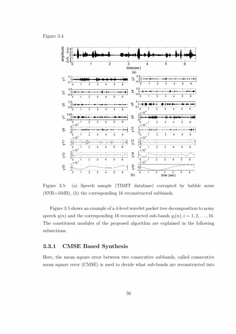
Figure 3.4.

Figure 3.5: (a) Speech sample (TIMIT database) corrupted by babble noise

(SNR=10dB), (b) the corresponding 16 reconstructed subbands.

Figure 3.5 shows an example of a 4-level wavelet packet tree decomposition to noisy

speech y(n) and the corresponding 16 reconstructed sub-bands yi(n), i = 1, 2, . . . , 16.

The constituent modules of the proposed algorithm are explained in the following

subsections.

3.3.1 CMSE Based Synthesis

Here, the mean square error between two consecutive subbands, called consecutive

mean square error (CMSE) is used to decide what sub-bands are reconstructed into

56

the HF band for Kalman filtering. The CMSE is defined as

Ek = CMSE(yk (n) , yk+1(n)) =1

N

N∑

n=1

(yk (n)− yk+1 (n))2 (3.16)

where k = 1, 2, . . . , 15 is the sub-band index, N is the number of the sub-band speech

samples. The underlying principle is to find k = js, the index of the last HF sub-band,

such that no significant difference between the two consecutive CMSE values, namely

Ejs and Ejs+1, is observed. Specifically, we compute Ek and Ek+1 for k = 1, 2, . . . , 15

until their difference is very small or negligible. Then such a value of k is denoted

as js. This empirical criterion is derived from extensive experiments. Once the value

of js is identified, the partially reconstructed HF and LF sub-band speeches are,

respectively, given by

yh (n) =

js∑

i=1

yi(n) (3.17)

yl (n) =16∑

i=js+1

yi(n) (3.18)

Figure 3.6 shows the CMSE values for the 16 sub-bands of the noisy speech y(n)

shown in Figure 3.5. From Figures 3.5 and 3.6, it is clearly observed that the 9th

Figure 3.6: The CMSE values corresponding to the sub-band speeches in Fig. 3.5.The double circle indicates the js.

subband is the last sub-band to be used for the partial reconstruction of the HF

band. In general, the value of js depends on the input speech samples, the noise

types, and the input SNR.

57

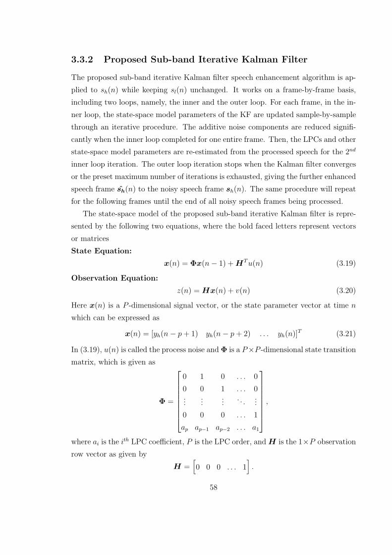
3.3.2 Proposed Sub-band Iterative Kalman Filter

The proposed sub-band iterative Kalman filter speech enhancement algorithm is ap-

plied to sh(n) while keeping sl(n) unchanged. It works on a frame-by-frame basis,

including two loops, namely, the inner and the outer loop. For each frame, in the in-

ner loop, the state-space model parameters of the KF are updated sample-by-sample

through an iterative procedure. The additive noise components are reduced signifi-

cantly when the inner loop completed for one entire frame. Then, the LPCs and other

state-space model parameters are re-estimated from the processed speech for the 2nd

inner loop iteration. The outer loop iteration stops when the Kalman filter converges

or the preset maximum number of iterations is exhausted, giving the further enhanced

speech frame sh(n) to the noisy speech frame sh(n). The same procedure will repeat

for the following frames until the end of all noisy speech frames being processed.

The state-space model of the proposed sub-band iterative Kalman filter is repre-

sented by the following two equations, where the bold faced letters represent vectors

or matrices

State Equation:

x(n) = Φx(n− 1) +HTu(n) (3.19)

Observation Equation:

z(n) = Hx(n) + v(n) (3.20)

Here x(n) is a P -dimensional signal vector, or the state parameter vector at time n

which can be expressed as

x(n) = [yh(n− p+ 1) yh(n− p+ 2) . . . yh(n)]T (3.21)

In (3.19), u(n) is called the process noise andΦ is a P×P -dimensional state transition

matrix, which is given as

Φ =

0 1 0 . . . 0

0 0 1 . . . 0...

......

. . ....

0 0 0 . . . 1

ap ap−1 ap−2 . . . a1

,

where ai is the ith LPC coefficient, P is the LPC order, and H is the 1×P observation

row vector as given by

H =[

0 0 0 . . . 1]

.

58

In (3.20), z(n) is the observation measurement of the state-space model at time n

and v(n) is the measurement noise.

For each frame of N samples, we set D as the maximum number of iterations.

The proposed iterative KF based speech enhancement can be summarized below.

Estimate LPCs ak, k = 1, 2, 3, . . . , P , from the sub-band noisy speech z(n). Let

sh(0) = z(n), n = 1, 2, 3, . . . , N .

For j = 1 to D do [outer loop]

Initialization:

x(j)(0|0) = 0 (3.22)

Σx(j)(0|0) = [0]p×p (3.23)

Φ(j) =

0 1 0 . . . 0

0 0 1 . . . 0...

......

. . ....

0 0 0 . . . 1

ap ap−1 ap−2 . . . a1

(3.24)

For n = 1 to N do [inner loop]

Time update (predictor):

x(j)(n|n− 1) = Φ(j)

x(j)(n− 1|n− 1) (3.25)

Σx(j)(n|n− 1) = Φ(j)Σx

(j)(n− 1|n− 1)Φ(j)T +HTσ2

uH (3.26)

Measurement update (corrector):

e(j)(n) = sh(j−1) −Hx

(j)(n|n− 1) (3.27)

K(j)(n) = [Σx

(j)(n|n)HT (HΣx(j)(n|n)HT

+ σ2v)

−1]HT (3.28)

x(j)(n|n) = x

(j)(n|n− 1) +K(j)(n)e(j)(n) (3.29)

Σx(j)(n|n) = (I −K

(j)(n)H)Σx(j)(n|n− 1) (3.30)

Estimate enhanced speech (at time n):

sh(j)(n) = Hx

(j)(n|n) (3.31)

59

End for [inner loop]

If |1− k(j)1 ||aP | < 1 (where k

(j)1 is the 1st element of K(j)(n)) [KF Converges]

Output the enhanced speech sh(n) and stop.

End for [outer loop]

Else

Re-estimate LPCs from the jth processed frame sh(j)(n), giving a new set of

ak’s, k = 1, 2, 3, . . . , P .

Repeat for [outer loop]

The above procedure is repeated for the following frames and continued until the

last frame being processed, resulting in ultimate enhanced speech sh(n) for all the

frames. Finally, the full-band enhanced speech s(n) is obtained as

s(n) = sh(n) + yl(n) (3.32)

3.3.3 Parameter Estimation

The LPC coefficients used in the sub-band iterative Kalman filter are updated based

on the partially enhanced speech in each frame for a better accuracy. In addition, it

can preserve the formant frequencies of the speech more precisely. Figure 3.7 shows

the estimated spectra (dashed), which can preserve the shapes of all the four formants

as compared to the clean speech spectra (solid).

As mentioned earlier, the noise variance σ2v is estimated from yh(n) rather than the

full-band noisy speech y(n), since yh(n) contains the vast majority of the additive noise

components. Noted that the noise variance estimated using the proposed algorithm

is already presented in section 2.4.1. Accordingly, we apply the difference operation

to yh(n), namely,

yh(n) =1

M

M−1∑

i=0

w[i]yh[n− i] (3.33)

where w is the derivative template (Table 1, chapter 2) and M is the length of w.

Finally, σ2v is estimated from yh(n) using the sample variance formula,

σ2v =

1

N

N∑

n=1

(yh(n)− µ)2 (3.34)

60

Figure 3.7: Power spectra comparison between the clean speech (solid), degradedspeech (dotted), and estimated (SBIT-KF) speech (dashed) in the presence of babblenoise (SNR = 0dB).

where µ is the sample mean of yh(n) and N is the number of sample points in the

analysis speech.

Figure 3.8 shows the performance comparison between the original noise variance

and the estimated noise variances obtained from the partially reconstructed HF sub-

band speech yh(n) and full-band noisy speech y(n), in the presence of white Gaussian

and non-stationary noises (input SNR=-5dB), respectively.

From Figure 3.8, it is observed that the noise variance σ2v of the additive noise

v(n) estimated from yh(n) approaches closely to the original noise variance, even at

low input SNR (-5dB) in both noise types. The noise variance estimated from the

full-band noisy speech y(n), on the other hand, deviates a bit from the original noise

variance.

3.4 Performance of the Proposed Method

In this simulation study, the same simulation setup as in section 2.6 is used. In addi-

tion, the Wavelet function used in the computation of the wavelet filter-bank is sym13,

order-13 least asymmetric orthogonal wavelet [62]. The proposed sub-band iterative

61

(a)

(b)

Figure 3.8: Performance comparison between the original and estimated noise vari-ances obtained from the partially reconstructed sub-band speech yh(n) and full-bandnoisy speech y(n), respectively, (a) white Gaussian, (b) non-stationary noise experi-ment. Speech utterances are taken from the TIMIT database (input SNR=-5dB).

62

Kalman filter based method (Proposed-SBIT-KF) is evaluated and compared with

the proposed iterative KF (Proposed-IT-KF), non-iterative KF (Proposed-NIT-KF)

and the existing methods, namely, LPCs enhancement in iterative Kalman filtering

(LPC-IT-KF) [26] and fast converging iterative Kalman filtering based method (FC-

IT-KF) [25].

Figure 3.9: Performance comparison between the proposed methods and other exist-

ing competitive methods in terms of PESQ. The speech utterances are corrupted by

(a): White, (b): Babble and (c): Car noises for a wide range of input SNRs(-10dB to

15dB).

From Figure 3.9, it is seen that the proposed sub-band iterative KF based method

performs better than the proposed non-iterative and iterative KF as well as the ex-

isting methods consistently, in terms of PESQ for all the three types of noises. In

addition, the performance of the existing competitive methods is worse than all the

three proposed methods at all input SNRs. This is attributed to the good overall

reduction of background noise, residual noise and distortion. More detailed simula-

tion results of the proposed methods in the presence of other adverse environmental

noises will be shown and discussed in Chapter 4.

63

3.5 Conclusion

In this chapter, at first, some background materials, including wavelet and filter-bank,

two-channel PR filter-bank, M -channel PR filter-bank, and wavelet packet tree de-

composition, have been introduced. Although the iterative Kalman filter performs

well than non-iterative Kalman filter in chapter 2, however, some musical-like arti-

facts as well as a bit distortion still remains in the enhanced speech. For further

improving the SE results, this chapter introduced the proposed sub-band iterative

KF based proposed SE method, where a wavelet filter-bank is used first to decom-

pose the noisy speech into a set of sub-bands. A consecutive mean square error

(CMSE) based scheme has been proposed to make partial reconstruction of the HF

and LF sub-bands such that the iterative Kalman filter is applied to the partially

reconstructed HF sub-band speech only, while keeping the LF sub-bands unchanged.

Then the partial enhanced speech provided by the iterative Kalman filter is combined

with the partially reconstructed LF sub-band speech to reconstruct the full-band en-

hanced speech. In the proposed method, the state-space model parameters have been

estimated from the sub-band speech rather than the full-band noisy speech, which

provides better accuracy. In addition, in the proposed method, the iterative Kalman

filter is applied only to the partially reconstructed HF sub-band speech rather than

all the decomposed sub-bands as done in some existing sub-band Kalman filter based

methods in the literature. Therefore, our method can reduce the computational com-

plexity to a certain extent.

The experimental results show that the proposed method performs better than

the existing methods for different environmental noises. It is also observed that the

proposed sub-band KF method outperforms other two Kalman filter based methods

presented in chapter 2.

64

Chapter 4

Simulation Results and Discussions

4.1 Experimental Setup

To illustrate the efficiency of the proposed methods, extensive computer simulations

are conducted, where the clean speech sentences are taken from the NOIZEUS speech

corpus [1], and TIMIT database[63], respectively. The NOIZEUS speech corpus

database is composed of 30 phonetically balanced sentences belonging to six speakers.

30 speech utterances, including 15 male and 15 female speakers are also selected from

the TIMIT database. The duration of the sentences taken from both of the database

is in between 2 to 4 seconds. The experiments are performed in the presence of

9 types of noises, namely, the white Gaussian, non-stationary, restaurant, babble,

street, car, pink, train, and cockpit noises for a wide range of input SNRs (-10dB to

15dB). Among the noise samples, white Gaussian, babble, car, pink, and cockpit (f16)

are taken from the Noisex-92 database [54]. Restaurant, street, and train noises are

taken from the NOIZEUS speech corpus database [1], and the non-stationary noise

is computer generated. The speech and noise are sampled at 16 kHz. A rectangular

window of 32 milliseconds is used for framing the test speech and the LPC order

used here is 8. The proposed Kalman filter based speech enhancement algorithms

are implemented in time-domain, where the rectangular window is fitted well during

framing and no overlapping is considered. The whole experiments are performed in

Matlab 8.1.

65

4.2 Performance Evaluation Methods

As for the assessment of the enhanced speech quality, various objective measures,

namely, the perceptual evaluation of speech quality (PESQ), signal to noise ratio

(SNR), segmental SNR (seg. SNR), and Log-likelihood ratio (LLR) are used. The

detailed description of these evaluation metrics are given below.

PESQ: In recent years, perceptually motivated measures have been popularly used

in measuring the speech quality. The PESQ evaluation metric is widely accepted as

an industrial standard for objective voice quality evaluation according to the ITU-T

recommendation P.862 [55]. PESQ includes a complex sequence of processing steps

to produce a set of distortion scores as a function of time and frequency. A simplified

block-diagram of the PESQ is shown in Figure 4.1.

Figure 4.1: Simplified block-diagram of the PESQ evaluation.

PESQ uses a perceptual model to convert the input and the degraded speech into

an internal representation. The degraded speech is time-aligned with the original

signal to compensate for the delay that may be associated with the degradation. The

difference in the internal representations of the two signals is then used by the cog-

nitive model to estimate the PESQ score. PESQ takes values between 1 (worst) and

4.5 (best) [55, 64].

SNR: Signal-to-Noise Ratio (SNR) is one of the oldest and widely used objective

measures. It is defined as the ratio of signal power to the noise power, often ex-

pressed in decibels. A ratio higher than 1:1 (greater than 0 dB) indicates more signal

than noise. It is mathematically simple to calculate, but requires both distorted and

66

undistorted (clean) speech samples [2, 64]. SNR can be calculated as follows

SNR = 10log10

∑Nn=1 s

2(n)∑N

n=1 [s(n)− s(n)]2(4.1)

where s(n) is the clean speech, s(n) is the distorted speech, and N the number of

samples.

Segmental SNR: The classical definition of SNR is not well related to the speech

quality for a wide range of distortions. To have a more complete evaluation of the

noise reduction performance, we also consider the segmental SNR, which correlates

well with the level of noise reduction regardless of the existing distortion in the speech.

In addition, it is less sensitive to the misalignments between the original and distorted

speech which occurs during the global SNR calculation. Therefore, it is an efficient

performance evaluation metric for the speech enhancement algorithm than the global

SNR [64]. Segmental SNR is calculated in short frames, and then averaged over a

number of frames [2, 64]. It is defined as

SegSNR =10

M

M−1∑

m=0

log10

∑Lm+L−1n=Lm s2(n)

∑Lm+L−1n=Lm [s(n)− s(n)]2

(4.2)

where L is the frame length (number of samples), and M the number of frames in

the signal (N = ML).

The frame length is normally set between 15 to 20 ms. Since the logarithm of

the ratio is calculated before averaging, the frames with an exceptionally large ratio

is somewhat weighed less, while frames with low ratio is weighed somewhat higher.

It can be observed that this matches the perceptual quality well, i.e., frames with

large speech and no audible noise does not dominate the overall perceptual quality,

but the existence of noisy frames stands out and will drive the overall quality lower.

However, if the speech sample contains excessive silence, the overall segmental SNR

values will decrease significantly, since silent frames generally show large negative

segmental SNR values. In this case, silent portions should be excluded from the

averaging using speech activity detectors. In the same manner, exclusion of frames

with excessively large or small values from averaging generally results in segmental

SNR values that agree well with the subjective quality [2]. A typical value for the

upper and the lower ratio limit is 35 and 10 dB [64].

LLR: The LLR is also used in this work as it is an important tool for measuring

67

the efficiency of the enhanced speech. It is a distance measure that can be directly

calculated from the LPC vector of the clean and distorted speech [64]. Therefore, it

is also called an LPC based object measure. It is calculated as follows

LLR = log(A

Te RcAe

ATc RcAc

) (4.3)

where Ac is the LPC vector for the clean speech, Ae is the LPC vector for the

enhanced speech, AT is the transpose of A, and Rc is the auto-correlation matrix for

the clean speech.

The less value of the LLR means that the enhanced speech contains less distortion

as well as better SNR improvement [64].

4.3 Performance Comparisons between the Pro-

posed and Existing Methods

The performances of the proposed methods are evaluated and compared against some

existing state-of-the art speech enhancement methods in terms of the aforementioned

evaluation metrics. In the first comparative study, 30 speech utterances are taken

from the TIMIT database and the experiment is performed in the presence of white

Gaussian, F16 Cockpit, and babble noises for a wide range of input SNRs(-10dB to

15dB). The performance of the Proposed-NIT-KF, Proposed-IT-KF, and Proposed-

SBIT-KF are compared with the existing competitive methods, namely, the bivariate

two-channel DWT (TC-DWT), three-channel double density DWT (TCDD-DWT),

higher-density discrete wavelet(HD-DWT), and four-channel double density discrete

wavelet transformation (FCHDD-DWT) based methods introduced by Hamid Reza

Tohidypour et all. in 2015 [42].

The experimental results presented in Figure 4.2 reveal that the proposed methods

consistently outperform the existing methods in terms of segmental SNR (dB) for

all the three noise types. Overall, the proposed sub-band iterative KF gives the

best result, then followed by the proposed iterative and the non-iterative KF based

methods, but all the three proposed methods perform much better for all input SNRs

than the existing methods. In particular, the existing methods provide very poor

performance at low input SNRs. At high input SNRs, although the existing methods

perform relatively well, yet not as good as the proposed methods.

68

Figure 4.2: Performance comparison between the proposed and existing competitivemethods in terms segmental SNR (dB). The speech utterances are corrupted by (a):White, (b):F16 Cockpit, and (c): Babble noises for a wide range for input SNRs(-10dBto 15dB).

Figure 4.3: Performance comparison between the proposed and existing methods interms of PESQ. The speech utterances are corrupted by (a): White, (b): F16 Cockpit,and (c): Babble noises for a wide range for input SNRs(-10dB to 15dB).

69

The PESQ results shown in Figure 4.3 indicates that the proposed methods per-

form better for all input SNRs in the three noisy cases than the existing methods.

It is also observed that the PESQ results of the existing methods below 1 at low

input SNRs, which is termed as the worst performance according to the ITU-T stan-

dard of PESQ [55]. Among the existing methods, FCHDD-DWT relatively performs

well than others. However, the average PESQ of FCHDD-DWT is still lower than the

proposed non-iterative KF based method which provides relatively lower performance

among the proposed methods.

To illustrate the efficiency of the proposed methods in the presence of other en-

vironmental noises, such as car, street, train, and restaurant noises, another experi-

ment is performed, where the speech samples are taken from NOIZEUS speech corpus

database [1]. The experiments are conducted for a wide range of input SNRs (0dB

to 15dB). The experimental results of the proposed methods (Proposed-NIT-KF,

Proposed-IT-KF,and Proposed-SBIT-KF) are compared with the existing methods,

namely the Wiener filter and harmonic regeneration based combined method (WF-

HRG), sub-band Wiener filter (SB-WF), and Wiener filter (WF) based methods in-

troduced by Ch.V. Rama Rao et all. in 2012 [36] in terms of the segmental SNR (dB)

and PESQ.

The segmental SNR (dB) results shown in Figure 4.4 reveal that the proposed

methods outperform existing Wiener filter based methods for all input SNRs in the

four noisy cases. It is also observed that the proposed methods always provide positive

segmental SNR improvement, even at low input SNRs for all the experiments. The

Wiener filter based methods, on the other hand, provide very poor performance at low

input SNRs, even the improved segmental SNRs are negative for all noise experiments.

In addition, at high input SNRs, such as at 15dB, the improved segmental SNRs of

the existing methods are less than 5dB, while for the proposed methods, it is greater

than 10dB which is regarded as excellent performance. In general, the higher value

of the segmental SNR (dB) indicates the weaker speech distortions as well as better

perceived quality in the enhanced speech. Through the extensive simulation results,

it is clearly observed that the proposed methods noticed lowest distortion in the

enhanced speech for all the four experiments than the existing methods.

From Figure 4.5, it is seen that the proposed methods provide significant PESQ

improvement than the existing Wiener filter based methods for all input SNRs of the

70

Figure 4.4: Performance comparison between the proposed and other existing meth-ods in terms of segmental SNR (dB). The speech utterances are corrupted by (a):Car, (b):Street, (c): Train, and (d): Restaurant noises for a wide range of inputSNRs(0dB to 15dB).

Figure 4.5: Performance comparison between the proposed and other existing meth-ods in terms of PESQ. The speech utterances are corrupted by (a): Car, (b): Street,(c): Train, and (d): Restaurant noises for a wide range of input SNRs(0dB to 15dB).

71

four noise experiments. It is also noted that at low input SNR, say at 0dB, the PESQ

improvement of the existing methods is close to 1, while it is greater than 2 for the

proposed methods. At high input SNR, say at 10dB, a significant PESQ improvement

is found for the proposed methods (always above 3) as opposed to existing methods

(always below 3) for all the four experiments. Among the proposed methods, the

sub-band iterative KF, followed by the iterative and non-iterative KF outperform the

existing Wiener filter based methods for all the four experiments.

4.4 Comprehensive Performance Comparisons be-

tween the Proposed Methods

To illustrate graphically the efficiency achieved by the proposed methods, the spec-

trograms for the clean, noisy and enhanced speech in the presence of white Gaussian

and non-stationary noises at 5dB input SNR are shown in Figure 4.6 and Figure 4.7

respectively.

From Figures 4.6 and 4.7, it is shown that there is a little bit residual noise

remaining in the enhanced speech provided by the non-iterative KF based method,

while noticeable improvement is found for the iterative KF. For sub-band iterative

KF, it removes the wide-band residual noise components significantly in the enhanced

speech and provides a better resolution in the speech spectral peaks and a very low

residual noise floor in the enhanced speech.

To illustrate the efficiency of the proposed methods in terms of the four evaluation

metrics, a comprehensive simulation study is conducted in the presence of 9 types of

noises for the SNR range of -10dB to 15dB. For performing these experiments, 30

speech sentences are taken from the TIMIT database. The main goal of this simu-

lation study is to show that the proposed methods perform the best across different

environmental noises, where most of the speech conversations take place.

The segmental SNR results presented in Figure 4.8 indicates that the sub-band

iterative KF relatively performs better for all noise experiments as compared to the

iterative and non-iterative KF. However, the iterative and non-iterative KF also pro-

vide noticeable segmental SNR improvement for all experiments.

The PESQ results presented in Figure 4.9 also indicates that the sub-band iterative

KF performs much better than other two proposed methods. Specifically, at 15dB

72

Figure 4.6: Spectrograms of (a): clean speech, (b): noisy speech, and enhancedspeech (c,d,e) obtained through using the Proposed-NIT-KF, Proposed-IT-KF, andProposed-SBIT-KF, respectively in the presence of white Gaussian noise (inputSNR=5dB).

73

Figure 4.7: Spectrograms of (a): clean speech, (b): noisy speech, and enhancedspeech (c,d,e) obtained through using the Proposed-NIT-KF, Proposed-IT-KF, andProposed-SBIT-KF, respectively in the presence of non-stationary noise (inputSNR=5dB).

74

Figure 4.8: Performance comparison between the proposed methods in terms of seg-mental SNR (dB) for a wide range of input SNRs (-10dB to 15dB) in the presence of9 types of noises.

75

Figure 4.9: Performance comparison between the proposed methods in terms of PESQfor a wide range of input SNRs (-10dB to 15dB) in the presence of 9 types of noises.

76

Figure 4.10: Performance comparison between the proposed methods in terms ofoutput SNR (dB) for a wide range of input SNRs (-10dB to 15dB) in the presence of9 types of noises.

77

Figure 4.11: Performance comparison between the proposed methods in terms of LLRfor a wide range of input SNRs (-10dB to 15dB) in the presence of 9 types of noises.

78

input SNR, the average PESQ for the sub-band iterative KF is greater than 3.5 for

all experiments, while at -10dB input SNR, it is still greater than 2, which ensures

a good quality of the enhanced speech. Although, the iterative KF provides better

performance than non-iterative KF, it introduces a little bit residual noise in the

enhanced speech. Therefore, the PESQ score of the iterative KF is relatively lower

than the sub-band iterative KF. The non-iterative KF, on the other hand, provides

relatively lower PESQ than the other two proposed methods, but it still performs

well across all the 9 types of noises.

The output SNR (dB) comparison results among the proposed methods are pre-

sented in Figure 4.10, where as usual, the sub-band iterative KF provides better

output SNR in the enhanced speech as compared to other two proposed methods.

For example, at 15dB input SNR, the output SNR (dB) provided by the sub-band

iterative KF is around 20dB, which is regarded as better competitive performance

in terms of output SNR (dB) improvement. At low input SNR, say at -10dB, there

we have also found noticeable output SNR(dB) improvement. The iterative KF also

performs well across all input SNRs and of course not as good as the sub-band iter-

ative KF. The output SNR (dB) results for the non-iterative KF is relatively lower

than the other two proposed methods. However, it still works well across all noise

experiments.

The LLR performance comparisons between the proposed methods are shown

in Figure 4.11. It also measures the amount of distortion in the enhanced speech.

As mentioned earlier, a lower LLR value indicates a lower speech distortion level,

which ultimately preserves good quality in the enhanced speech. Again, the sub-

band iterative KF provides the lowest LLR for all the experiments even at a low

input SNR, which is followed by the iterative and non-iterative KF.

4.5 Computational Complexity

The computational complexity of the proposed algorithms depends on a couple of

things, namely, the LPC order to be used, the number of iterations for the itarative

Kalman filter to be converged and the level of input SNRs. Through extensive simu-

lations, it is observed that the proposed iterative Kalman filter normally convereges

after 3 iterations, while the sub-band iterative Kalman filter converges at the second

79

iteration. The existing iterative Kalman filter methods, on the other hand, converges

after 4-5 iterations. In order to fix the LPC order, an experiment is performed for

different LPC order versus the CPU computational times and the PESQ results for

each LPC order. For this experiment, 30 speech utterances are taken from TIMIT

database. The experiment is performed in the presence of restaurant noise with 10dB

input SNR. The simulation is conducted on a computer with Windows 7 (64-bit),

6GB RAM, Intel corei 7 processor having CPU speed of 2.40 GHz. The experimental

results are shown in Figure 4.12.

From Figure 4.12, it is observed that, as the LPC order increases, a minor increase

of PESQ results is found for the three proposed methods but the CPU computational

time (sec) increases dramatically. Since the iterative KF converges after 3 iterations,

the computational time for iterative KF is logically three times larger than the non-

iterative KF as shown in Figure 4.12. For the same reason, the computational time

for sub-band iterative KF is two times larger than non-iterative KF. However, con-

sidering the trade off between computational complexity and speech enhancement

performance, we set the LPC order 8 in the overall simulation study.

It is important to note that, the computational time of the proposed methods for

different levels of input SNR (-10dB to 15dB) varies slightly. In general, it is observed

that the non-iterative KF takes less computational time followed by the sub-band

iterative KF and then the iterative KF, respectively. However, the sub-band iterative

KF performs better than the iterative and non-iterative KF based methods.

80

Figure 4.12: Computational complexity comparison of the proposed methods, (a):

CPU time (sec) versus LPC order and (b): PESQ versus LPC order in the presence

of restaurant noise (input SNR=10dB).

81

4.6 Conclusion

In this chapter, an extensive simulation study has been conducted for the evaluation

of the proposed methods in the presence of 9 different types of noises for a wide

range of input SNRs. The performances have been evaluated and compared with

some of the existing methods in terms of four evaluation metrics. The experimental

results reveal that the proposed methods provide very good performance in terms

of all the performance metrics with the consumption of a resonable amount of CPU

computational time. Through the extensive experimental results, it is also shown that

the proposed methods perform much better for different environmental noises than

the other existing competitive methods whose performances are limited to particular

types of noises as mentioned in the literature. In addition, among the proposed

methods, the sub-band iterative Kalman filter performs the best, followed by the

iterative and non-iterative Kalman filter based methods, respectively, for all the noisy

cases in terms of all the evaluation metrics.

82

Chapter 5

Conclusion

5.1 Summary of the Work

In this thesis, Kalman filter based single channel speech enhancement algorithms that

are capable of dealing with adverse environmental noises have been investigated. The

proposed algorithms have been implemented in non ideal cases, where the state-space

model parameters of the Kalman filter, namely, the LPC and noise variance are es-

timated in noisy conditions without considering any a priori knowledge of the clean

speech and the additive noise. In most of the existing Kalman filter based methods,

however, the clean speech and noise information are assumed to be available for these

parameter estimation. These prior assumptions make these algorithms impractical

in the sense that in real speech enhancement scenarios, we can access only the noisy

speech. In order to resolve these issues, new methods for LPC and noise variance

estimation in noisy conditions have been proposed. Depending on these parame-

ter estimation techniques, three Kalman filter based speech enhancement methods

operating on a frame-by-frame basis have been developed.

First, in the non-iterative Kalman filter based method, the state-space model

parameters, namely, LPCs and noise variance are estimated in noisy conditions. A

combined speech smoothing and autocorrelation method has been proposed for LPC

estimation. A new method based on a truncated Taylor series expansion of the noisy

speech along with a difference operation serving as high-pass filtering is introduced

for the noise variance estimation. It has been shown that the proposed non-iterative

Kalman filter is implemented effectively with these estimated parameters.

83

Although the non-iterative Kalman filter performs relatively well, yet it introduces

some residual noises and small distortions in the enhanced speech. In order to improve

the speech enhancement performance as well as parameter estimation accuracy in

noisy conditions, an iterative Kalman filter based method has been presented as

the second approach. For each frame, at first, the state-space model parameters of

the Kalman filter are estimated from the noisy speech. When the Kalman filtering

iteration has gone through the entire frame, the LPCs and other state-space model

parameters are re-estimated from the processed speech frame and the Kalman filter

is applied again to the same processed frame for further enhancement. The iteration

stops when the Kalman filter converges or when the preset maximum number of

iterations is exhausted, giving further enhanced speech frame corresponding to the

input noisy speech frame. The same procedure will repeat for the following frames

until the end of all noisy frames being processed.

Although the enhanced speech provided by the iterative Kalman filter is free from

residual noise that appear in the proposed non-iterative Kalman filter based method,

some musical-like artifacts do remain in the enhanced speech. For further improving

the speech enhancement results, a sub-band iterative Kalman filter has been pro-

posed as the third approach. A wavelet filter-bank is first used to decompose the

noisy speech into a number of sub-bands. To achieve the best trade-off among the

noise reduction, speech intelligibility and computational complexity, a partial recon-

struction scheme based on consecutive mean squared error (CMSE) is proposed to

synthesize the LF and HF sub-bands such that the iterative Kalman filter is employed

only to the partially reconstructed HF sub-band speech. Finally, the enhanced HF

sub-band speech is combined with the partially reconstructed LF sub-band speech to

reconstruct the full-band enhanced speech.

The proposed methods have been tested with two widely used speech databases,

namely, TIMIT and NOIZEUS corpus, respectively. The experiments have been con-

ducted in the presence of 9 types of noises for a wide range of input SNRs, where

real-life speech conversations often take place. The performances are evaluated and

compared against some state-of-the art speech enhancement methods. Through ex-

tensive simulations, it is clearly observed that the proposed methods are effective

in noise reduction, while preserving a good quality in the enhanced speech than ex-

isting competitive methods. The computational time for the proposed methods is

84

also resonable. In addition, the proposed methods can perform well in the presence

of different environmental noises, while the performances of some existing methods

are limited to specific types of noise. Among the proposed methods, the sub-band

iterative Kalman filter performs the best, followed by the iterative and non-iterative

Kalman filter in terms of the reported evaluation metrics.

5.2 Suggestions for Future Work

The proposed methods have been implemented for single channel speech enhance-

ment, where one noisy mixture gives the overall spectral information of the degraded

speech since there is only one microphone/channel available. In addition, the pro-

posed thesis considers only the noise reduction, where the room dereverberation, and

acoustic echo cancellation are not yet considered, which are also treated as the im-

portant environmental disturbance in the original acoustic environments. In order

to capture the noisy mixtures including the reverberation, and acoustic echo more

precisely, which exhibit some advantages in incorporating both the spatial and the

spectral information, the multi microphone/channel experimental environment plays

an important role. Therefore, the future direction of this research is to extend the

proposed Kalman filter based methods such that they are capable of working in the

multi channel/microphone environments, which is expected to reduce the additive

noise, the room reverberation, and acoustic echo efficiently.

85

Bibliography

[1] P.C. Loizou. Speech Enhancement: Theory and Practice. Signal processing and

communications. Taylor & Francis, 2007.

[2] K. Kondo. Subjective Quality Measurement of Speech its Evaluation, Estimation

and Application. Springer, 2012.

[3] Sheng-Chieh Lee, Bo-Wei Chen, and Jhing-Fa Wang. Noisy environment-aware

speech enhancement for speech recognition in human-robot interaction applica-

tion. In IEEE International Conference on Systems Man and Cybernetics (SMC),

pages 3938–3941, Oct 2010.

[4] B.H. Juang. Ubiquitous speech communication interface. In IEEE Workshop on

Automatic Speech Recognition and Understanding,, pages 85–92, 2001.

[5] N. Magotra, F. Livingston, and S. Rajagopalan. Single channel speech enhance-

ment in real time. In The Twenty-Seventh Asilomar Conference on Signals,

Systems and Computers, volume 2, pages 1211–1215, Nov 1993.

[6] B.-G. Lee, K.Y. Lee, S. Ann, and Iickho Song. A sequential algorithm for robust

parameter estimation and enhancement of noisy speech. In IEEE International

Symposium on Circuits and Systems (ISCAS), volume 1, pages 243–246, May

1993.

[7] Manfred R. Schroeder. Apparatus for suppressing noise and distortion in com-

munication signals, April 27 1965. US Patent 3,180,936.

[8] J.R. Jensen, J. Benesty, M.G. Christensen, and S.H. Jensen. Enhancement of

single-channel periodic signals in the time-domain. IEEE Transactions on Audio,

Speech, and Language Processing, 20(7):1948–1963, Sept 2012.

86

[9] J.S. Lim and A.V. Oppenheim. All-pole modeling of degraded speech. IEEE

Transactions on Acoustics, Speech and Signal Processing, 26(3):197–210, Jun

1978.

[10] J.S. Lim and A.V. Oppenheim. Enhancement and bandwidth compression of

noisy speech. Proceedings of the IEEE, 67(12):1586–1604, Dec 1979.

[11] Y. Kuroiwa and T. Shimamura. An improvement of lpc based on noise reduction

using pitch synchronous addition. In IEEE International Symposium on Circuits

and Systems (ISCAS), volume 3, pages 122–125, Jul 1999.

[12] Rudolph Emil Kalman. A new approach to linear filtering and prediction prob-

lems. Transactions of the ASME–Journal of Basic Engineering, 82(Series D):35–

45, 1960.

[13] K.K. Paliwal and A. Basu. A speech enhancement method based on kalman

filtering. In IEEE International Conference on Acoustics, Speech, and Signal

Processing (ICASSP), volume 12, pages 177–180, Apr 1987.

[14] E.A. Wan and A.T. Nelson. Neural dual extended kalman filtering: applications

in speech enhancement and monaural blind signal separation. In Proceedings of

the IEEE Workshop on Neural Networks for Signal Processing, pages 466–475,

Sep 1997.

[15] S. Gannot, D. Burshtein, and E. Weinstein. Iterative and sequential kalman

filter-based speech enhancement algorithms. IEEE Transactions on Speech and

Audio Processing, 6(4):373–385, Jul 1998.

[16] M. Gabrea. An adaptive kalman filter for the enhancement of speech signals in

colored noise. In IEEE Workshop on Applications of Signal Processing to Audio

and Acoustics, pages 45–48, Oct 2005.

[17] Ning Ma, M. Bouchard, and R.A. Goubran. Perceptual kalman filtering for

speech enhancement in colored noise. In IEEE International Conference on

Acoustics, Speech, and Signal Processing (ICASSP), volume 1, pages I–717–720,

May 2004.

87

[18] Chang Huai You, S. Rahardja, and Soo Ngee Koh. Perceptual kalman filtering

speech enhancement. In IEEE International Conference on Acoustics, Speech

and Signal Processing (ICASSP), volume 1, pages I–461–464, May 2006.

[19] Yu Shao and Chip-Hong Chang. A kalman filter based on wavelet filter-bank

and psychoacoustic modeling for speech enhancement. In IEEE International

Symposium on Circuits and Systems (ISCAS), pages 121–124, May 2006.

[20] Quanshen Mai, Dongzhi He, Yibin Hou, and Zhangqin Huang. A fast adaptive

kalman filtering algorithm for speech enhancement. In IEEE Conference on

Automation Science and Engineering (CASE), pages 327–332, Aug 2011.

[21] R. Ishaq, B. Garcia Zapirain, M. Shahid, and B. Lovstrom. Subband modulator

kalman filtering for single channel speech enhancement. In IEEE International

Conference on Acoustics, Speech and Signal Processing (ICASSP), pages 7442–

7446, May 2013.

[22] Yu Wang and M. Brookes. Speech enhancement using a robust kalman filter

post-processor in the modulation domain. In IEEE International Conference on

Acoustics, Speech and Signal Processing (ICASSP), pages 7457–7461, May 2013.

[23] Naushin Nower, Yang Liu, and Masashi Unoki. Restoration scheme of instan-

taneous amplitude and phase using kalman filter with efficient linear prediction

for speech enhancement. Speech Communication, 70:13 – 27, 2015.

[24] J.D. Gibson, Boneung Koo, and S.D. Gray. Filtering of colored noise for speech

enhancement and coding. IEEE Transactions on Signal Processing, 39(8):1732–

1742, Aug 1991.

[25] Stephen So and Kuldip K. Paliwal. Fast converging iterative kalman filtering

for speech enhancement using long and overlapped tapered windows with large

side lobe attenuation. In 11th Annual Conference of the International Speech

Communication Association (INTERSPEECH), pages 1081–1084, Sep 2010.

[26] T. Mellahi and R. Hamdi. Lpcs enhancement in iterative kalman filtering for

speech enhancement using overlapped frames. In International Conference on

Electrical Sciences and Technologies in Maghreb (CISTEM), pages 1–5, Nov

2014.

88

[27] S.M. McOlash, Russell J. Niederjohn, and James A. Heinen. A spectral subtrac-

tion method for the enhancement of speech corrupted by nonwhite, nonstationary

noise. In IEEE 21st International Conference on Industrial Electronics, Control,

and Instrumentation (IECON), volume 2, pages 872–877, Nov 1995.

[28] D.J. Darlington and D.R. Campbell. The effect of modified filter distribution

on an adaptive, sub-band speech enhancement method. In IEEE Digital Signal

Processing Workshop, pages 153–156, Sep 1996.

[29] Y. Malca and D. Wulich. Improved spectral subtraction for speech enhancement.

In 8th European Signal Processing Conference (EUSIPCO), pages 1–5, Sept 1996.

[30] S. Ayat, M.T. Manzuri, R. Dianat, and J. Kabudian. An improved spectral sub-

traction speech enhancement system by using an adaptive spectral estimator. In

Canadian Conference on Electrical and Computer Engineering (CCECE), pages

261–264, May 2005.

[31] Ning Cheng, Wen-Ju Liu, and Bo Xu. An improved a priori mmse spectral

subtraction method for speech enhancement. In 3rd International Workshop on

Signal Design and Its Applications in Communications (IWSDA), pages 373–377,

Sept 2007.

[32] Lu ying Sui, Xiong wei Zhang, Jian jun Huang, and Bin Zhou. An improved

spectral subtraction speech enhancement algorithm under non-stationary noise.

In International Conference on Wireless Communications and Signal Processing

(WCSP), pages 1–5, Nov 2011.

[33] Liang Cao, Tian-qi Zhang, Hong-xing Gao, and Chen Yi. Multi-band spec-

tral subtraction method combined with auditory masking properties for speech

enhancement. In 5th International Congress on Image and Signal Processing

(CISP), pages 72–76, Oct 2012.

[34] K. Funaki. Speech enhancement based on iterative wiener filter using complex

speech analysis. In 16th European Signal Processing Conference, pages 1–5, Aug

2008.

[35] C.V.R. Rao, M.B.R. Murthy, and K.S. Rao. Speech enhancement using per-

ceptual wiener filter combined with unvoiced speech-a new scheme. In IEEE

89

Conference on Recent Advances in Intelligent Computational Systems (RAICS),

pages 688–691, Sept 2011.

[36] Ch.V. Rama Rao, M.B. Rama Murthy, and K. Srinivasa Rao. Speech enhance-

ment using sub-band cross-correlation compensated wiener filter combined with

harmonic regeneration. {AEU} - International Journal of Electronics and Com-

munications, 66(6):459 – 464, 2012.

[37] V. Sunnydayal and T.K. Kumar. Speech enhancement using sub-band wiener

filter with pitch synchronous analysis. In International Conference on Advances

in Computing, Communications and Informatics (ICACCI), pages 20–25, Aug

2013.

[38] Jong Won Seok and Keun Sung Bae. Speech enhancement with reduction of

noise components in the wavelet domain. In IEEE International Conference on

Acoustics, Speech, and Signal Processing (ICASSP), volume 2, pages 1323–1326,

Apr 1997.

[39] M. Bahoura and Jean Rouat. Wavelet speech enhancement based on the teager

energy operator. IEEE Signal Processing Letters, 8(1):10–12, Jan 2001.

[40] M.S. Arefeen Zilany, M.K. Hasan, and M. Rezwan Khan. Efficient hard and soft

thresholding for wavelet speech enhancement. In 11th European Signal Processing

Conference, pages 1–4, Sept 2002.

[41] A. Parajuli and V. DeBrunner. Speech enhancement using perceptual wavelet

thresholding with the ephraim and malah noise suppressor and auditory masking.

In 39th Asilomar Conference on Signals, Systems and Computers, pages 301–304,

Oct 2005.

[42] Hamid Reza Tohidypour and Seyed Mohammad Ahadi. New features for speech

enhancement using bivariate shrinkage based on redundant wavelet filter-banks.

Computer Speech & Language, 35:93–115, Jan 2016.

[43] P. Rubin and E. Vatikiotis-Bateson. Measuring and Modeling Speech Production.

Springer Berlin Heidelberg, 1998.

90

[44] Lawrence R. Rabiner and Ronald W. Schafer. Introduction to digital speech

processing. Foundations and Trends in Signal Processing, 1(12):1–194, 2007.

[45] Jacob Benesty, M. Mohan Sondhi, and Yiteng (Arden) Huang. Springer Hand-

book of Speech Processing. Springer-Verlag New York, Inc., Secaucus, NJ, USA,

2007.

[46] Saeed V. Vaseghi. Advanced Digital Signal Processing and Noise Reduction. John

Wiley & Sons, 2006.

[47] A. Trabelsi, F.R. Boyer, Y. Savaria, and M. Boukadoum. Improving lpc analysis

of speech in additive noise. In IEEE Northeast Workshop on Circuits and Systems

(NEWCAS), pages 93–96, Aug 2007.

[48] Qifang Zhao, Tetsuya Shimamura, and Jouji Suzuki. Improvement of lpc analysis

of speech by noise compensation. Electronics and Communications in Japan

(Part III: Fundamental Electronic Science), 83(9):73–83, 2000.

[49] H.T. Hu. Linear prediction analysis of speech signals in the presence of white

gaussian noise with unknown variance. IEE Proceedings-Vision, Image and Sig-

nal Processing, 145(4):303–308, Aug 1998.

[50] S.M. Kay. Noise compensation for autoregressive spectral estimates. IEEE Trans-

actions on Acoustics, Speech and Signal Processing, 29(3):292–303, Jun 2003.

[51] P.J. Hargrave. A tutorial introduction to kalman filtering. In IEE Colloquium

on Kalman Filters: Introduction, Applications and Future Developments, pages

1/1–1/6, Feb 1989.

[52] Greg Welch and Gary Bishop. An introduction to the kalman filter. Technical

report, Chapel Hill, NC, USA, 1995.

[53] T. O’Haver. A pragmatic introduction to signal processing with applications

in scientific measurement, University of Maryland, USA, July 2015, Available:

https://terpconnect.umd.edu/ toh/spectrum/TOC.html.

[54] Andrew Varga and Herman J.M. Steeneken. Assessment for automatic speech

recognition: Ii. noisex-92: A database and an experiment to study the effect of

91

additive noise on speech recognition systems. Speech Communication, 12(3):247

– 251, 1993.

[55] A. W. Rix, J. G. Beerends, M. P. Hollier, and A. P. Hekstra. Perceptual eval-

uation of speech quality (pesq)-a new method for speech quality assessment of

telephone networks and codecs. In IEEE International Conference on Acoustics,

Speech, and Signal Processing (ICASSP), pages 749–752, Washington, DC, USA,

2001.

[56] M. Vetterli and C. Herley. Wavelets and filter banks: theory and design. IEEE

Transactions on Signal Processing, 40(9):2207–2232, Sep 1992.

[57] Iman Moazzen and Pan Agathoklis. A general approach for filter bank design

using optimization. Technical report, Department of Electrical and Computer

Engineering University of Victoria, Victoria, B.C. Canada, March 2014.

[58] P.P. Vaidyanathan. Multirate digital filters, filter banks, polyphase networks,

and applications: a tutorial. Proceedings of the IEEE, 78(1):56–93, Jan 1990.

[59] Truong Q. Nguyen. A tutorial on filter banks and wavelets, 1995, available:

citeseer.nj.nec.com/nguyen95tutorial.html.

[60] Robi Polikar. The engineer’s ultimate guide to wavelet analysis-the wavelet tuto-

rial, 1996, available: http://users.rowan.edu/ polikar/wavelets/wttutorial.html.

[61] Wan-lu Jiang. Orthogonal wavelet packet analysis based chaos recognition

method. Frontiers of Electrical and Electronic Engineering in China, 1(1):13–19,

2006.

[62] Ingrid Daubechies. Orthonormal bases of compactly supported wavelets. Com-

munications on Pure and Applied Mathematics, 41(7):909–996, 1988.

[63] John S Garofolo, Linguistic Data Consortium, et al. TIMIT: acoustic-phonetic

continuous speech corpus. Linguistic Data Consortium, 1993.

[64] Yi Hu and P.C. Loizou. Evaluation of objective quality measures for speech

enhancement. IEEE Transactions on Audio, Speech, and Language Processing,

16(1):229–238, Jan 2008.

92