single-well imaging using full waveform sonic data - · pdf filesingle-well imaging using full...

Single-well imaging

CREWES Research Report � Volume 14 (2002) 1

Single-well imaging using full waveform sonic data

Louis Chabot, R. James Brown, David C. Henley, and John C. Bancroft,

ABSTRACT The sonic-waveform processing and imaging flow presented in this paper uses full-

waveform data recorded with a conventional acoustic well-logging tool, then adapts known surface-seismic processing steps and optimizes them for the borehole environment. This paper presents improvements brought to our original sonic-waveform processing and imaging flow. These improvements are better geometry assignment, better noise attenuation, better data enhancement, and the application of prestack time migration with improved parameters. The new flow is tested on a portion of a full-waveform sonic dataset, recorded over a section of the 8-8-23-23W4 well, Blackfoot field, Alberta, intersecting three coal seams at an angle. The upper portion of the composite sonic image showed promising indications of dipping interfaces. However, the targeted three coal seams were not very well imaged in the final composite sonic image. This is probably because of the strong attenuation of the sonic energy by the fractured coal. The composite sonic image shows potentially better resolution than the coinciding surface seismic section. More work is planned to improve further on the demonstrated processing flow.

INTRODUCTION Acoustic well-logging is presently used for the following applications: formation

mechanical property analysis (e.g. elastic moduli), formation evaluation (e.g. lithology), geophysical interpretation (e.g. synthetic seismograms), and more recently, shear-wave anisotropy measurements. All of these applications are generated from the analysis of the full-waveform acquired by the acoustic well-logging tool.

The acoustic well-logging tool provides a unique geometry whereby both source and receivers are in the same wellbore, several receivers are located at different offsets along the body of the well-logging tool and, as the well-logging tool is moved uphole, the subsurface surrounding the wellbore is sampled repeatedly. This unique configuration can be analogous to a single-well imaging experiment.

Single-well imaging can be considered a subset of the many borehole seismic imaging techniques in use today. Single-well imaging can be defined as the study of the acoustic and elastic wave propagation in and around a borehole where the source and receivers are located in the same borehole. Single-well imaging data can be acquired in different ways: for example, using a borehole seismic source with clamped receivers in the same borehole to image the flank of a salt dome, or using an acoustic well-logging tool to evaluate the elastic properties of geologic formations. The focus of this work is on single-well imaging using a conventional acoustic well-logging tool.

Single-well imaging can contribute to reservoir understanding by bridging the resolution gap between well-logging and seismic data (Figure 1) by extending our understanding of the reservoir characteristics to an intermediate scale. In addition, this technique has the advantage of requiring only one borehole (in contrast to crosswell), one instrument (in contrast to vertical seismic profiling) and the full waveform data is

Chabot et al.

2 CREWES Research Report � Volume 14 (2002)

available wherever a dipole sonic is acquired (the full waveform is obtained simultaneously with the acquisition of the compressional and shear velocity logs). There have been previous attempts at single-well imaging using acoustic well-logging tools (Hornby, 1989; Fortin et al., 1991; Coates et al., 2000).

Hornby (1989) used an experimental acoustic well-logging tool equipped with one monopole source and twelve receivers, each recording 20 ms of full-waveform data, to compute an image of structural changes beyond the borehole wall. Details of the tool geometry are provided in Table 1. With the source and receiver array both passing through the structures that cross the borehole, downdip and updip structures could be imaged separately.

In his single-well imaging effort, Hornby (1989) removed the direct P-waves, P and S headwaves, as well as the Stoneley arrivals from the records using an f-k filter. Then, he applied a back-projection operator to the prestack velocity-filtered sonic data, followed by a common midpoint stack (6-fold). Finally, he migrated the data with a generalized Radon transform to image the scatter energy.

Table 1. Single-well imaging: tool geometries.

Prototype acoustic logging tool

EVA (Evaluation of velocity and attenuation)

BARS� (Borehole acoustic reflection

survey)

(Hornby, 1989) (Fortin et al., 1991) (Coates et al., 2000)

Number of transmitters

1 monopole 4 monopoles Up to 3 monopoles

Frequency band 5 - 18 kHz 3 � 25 kHz 8-30 kHz (?)

Number of receivers 12 12 8

Near to far offsets 3.35 to 5 m 1 to 12.75 m 9.75 to 13.10 m

Receiver spacing 0.15 m 1.00 m 0.30 m

Data sampling rate 20 µs 5 or 10 µs 10 µs (?)

Waveform recorded 20 ms 12.5 ms 12 ms

Shot spacing, or logging speed and shot firing rate.

0.15 m 6 m/min. (?)

6 m/min. (?)

Fortin et al. (1991) instead used an array sonic logging tool called the EVA� (evaluation of velocity and attenuation) designed with four transmitters and twelve receivers. Their processing flow consisted, in the shot-gather domain, in separating the reflection energy coming from above the well axis from the reflection energy coming from below the well axis. Once separated, two distinct gathers were created. The gathers were afterwards processed separately in the following fashion: velocity filtering of S-Rayleigh waves and of Stoneley waves, normal moveout and midpoint stack. Finally the two processed sections were put together along their zero line to form a sonic image. However, no migration was applied to the stacked image.

Single-well imaging


Coates et al. (2000) used a modified dipole shear-sonic imager (DSI�) tool or BARS� (borehole acoustic reflection survey) and generated imaging results for near-horizontal wells. Details of their full waveform processing are provided in Table 2.

Table 2. Single-well imaging: full waveform processing.

Prototype tool EVA (Evaluation of velocity and attenuation)

BARS� (Borehole acoustic reflection

survey)

(Hornby, 1989) (Fortin et al., 1991) (Coates et al., 2000)

Deconvolution No No No (?)

Static corrections No No No

Filtering Removal of direct P, refracted P and S (pseudo-Rayleigh), and Stoneley arrivals by f-k filtering

Removal of direct borehole arrivals by velocity filtering. Wavefield separation (updip and downdip)

Removal of direct borehole arrivals. Wavefield separation

Normal moveout Yes Yes Yes

Common midpoint stack

Yes (6 fold) Yes (16 fold) ?

Migration Prestack back-projection operator

No Conventional Kirchhoff

Angle between the borehole axis and the intersecting beds

43 degrees 15 to 35 degrees 0 degrees (near-horizontal well)

Imaging distance from borehole axis

18 m 7 m 10 m

This work investigates the acoustic and elastic-wave propagation in and around an open borehole, using the full waveform acquired with a conventional sonic logging tool, with the purpose of creating a processing-imaging flow applicable to full-waveform sonic data to image reflected energy originating from acoustic impedance contrasts from beyond the borehole walls. Those contrasts could be interpreted as structural changes, which could improve our knowledge of the reservoir not easily seen in the surface seismic.

Chabot et al.


FIG. 1: Single-well imaging bridging the resolution gap between well-logging and seismic data (Coates et al., 2000).

ACOUSTIC WAVE PROPAGATION IN AND AROUND THE BOREHOLE Individual acoustic waveform appearances (amplitude and phase) are dependent on:

source signal and frequency content, the characteristics of the logging tool, the borehole diameter (e.g. number and character of trapped modes), fluid properties, and formation properties. Paillet and Cheng (1991) explored those factors affecting full waveforms through the use of synthetic borehole micro-seismograms.

FIG. 2: Theoretical shot record acquired with an acoustic well-logging tool along the borehole axis (Coates et al., 2000).

Of particular interest to this work is the variation of acoustic energy with offset (Figure 2). There are compressional and shear headwaves, where the energy exhibits linear moveout. There are also interface waves (pseudo-Rayleigh and Stoneley waves), where the energy also exhibits linear moveout. The pseudo-Rayleigh and the shear headwaves have such similar velocities that they arrive too close to one another to be distinguished. Finally there is scattered energy coming from acoustic impedance contrast away from the borehole wall. The energy from headwaves and from interface waves has

Single-well imaging


a tendency to obscure either shallow reflections at large offsets or deeper reflections at smaller offsets. This leaves zones in the raw waveforms where the reflected energy could be observed (oval-shaded areas in Figure 2).

SIMPLIFICATION OF THE 3D BOREHOLE PROBLEM INTO A 2D BOREHOLE PROBLEM FOR SIMPLE SHAPES

The numerical modelling results were previously presented in which the proposed full-waveform processing flow was successfully tested on acoustic synthetic data from 2D borehole models (Chabot et al., 2001). Although a 3D finite-difference numerical-modelling package for modelling borehole wave propagation would have been ideal (Cheng et al., 1995; Liu, et al., 1996), none were made available to us at the time.

With the proposed waveform-processing flow successfully tested on 2D borehole models, efforts were made to seek exploitable geometries that would simplify the known 3D nature of the borehole environment into a 2D problem. Such exploitable geometries do exist.

Figure 3 shows a 3D volume (x, y, z) with a single dipping interface pierced by a vertical borehole. The source and receiver arrays are located vertically along the borehole axis. No borehole-fluid effects are included in this representation and the media above and below the interface are isotropic. In Figure 3, raytracing, as performed with the help of the NORSAR-3D� modelling software, illustrates the wavefield propagation in and around the borehole.

FIG. 3: Raytracing of a simple 3D borehole model (x, y, z) with a dipping interface (illustrated here with a dipping plane separating layers of different acoustic impedance) pierced by a vertical borehole. The vertical borehole is populated with arrays of receivers while the source is located above the interface. This view plots rays every 15° of azimuth and dip.

The results of simulations show that the reflected energy recorded at the receivers in the borehole is confined to the vertical plane subtended by the vertical borehole and the normal to the dipping interface. No other reflected energy from the dipping interface returns to the receiver arrays in the borehole and thus is never recorded. When the effects

Chabot et al.


of the borehole fluid are added to the model (not shown here), the reflected energy recorded at the receivers is again propagating within this same vertical plane, which also contains the direction of dip of the interface. From these results it can thus be shown, for simple single-well imaging geometries (Figure 3), that the 3D borehole problem can be simplified into a 2D problem by cutting the 3D volume with a vertical plane parallel to the dip direction of the interface and intersecting the borehole path.

ACQUISITION OF FULL-WAVEFORM FIELD DATA The full-waveform field dataset studied here was acquired in the 8-8-23-23W4 well

located in the Blackfoot field in Alberta. This dataset consists of 310 m of full-waveform data, acquired in the deviated section of the well that intersected, at an angle of 20° to 30° from the vertical, a flat-lying sequence of alternating sandstones, shales and limestones. The geology of the Blackfoot field is described in detail by Miller et al. (1995). The full-waveform data were acquired with a DSI� (Figure 4), a conventional well-logging tool, in a monopole configuration, with an acoustic bandwidth of 8 to 30 kHz. Receivers were located 15 cm apart on the tool with a near-offset distance to the source of 2.74 m and a far offset of 3.81 m. Eight full waveforms were recorded simultaneously at the firing of the monopole source to create a shot gather. Each waveform was recorded with a sampling interval of 10 µs for a total of 512 samples/waveform (Harrison et al., 1990).

FIG. 4: Diagram representing the tool geometry of the acoustic well-logging tool, DSI� (Schlumberger, 1997), that was used to acquire the full waveform dataset from the top of the Manville group to the Mississippian unconformity.

Figure 5 illustrates a sample of 5 consecutive shot gathers, of eight full waveforms each, taken from source depths of 1631.37 m to 1630.76 m in the well. A look at Figure 5 reveals the presence in the full waveforms of the compressional (4445 m/s), shear or pseudo-Rayleigh (2481 m/s) and Stoneley (1404 m/s) arrivals, all of which have linear moveout. These waveforms could also contain energy scattered from beyond the borehole wall. However, as can be seen in these raw shot records, because the energy with the

Single-well imaging


linear moveout is so much more prominent than the energy from reflections, it will make interpretation in the present form difficult. Thus we need to process the data.

FIG. 5: Identification of compressional (P), shear or pseudo-Rayleigh (S) and Stoneley (St) arrivals in a sample of five sonic shot gathers; vertical scale is in ms.

SONIC WAVEFORM PROCESSING AND IMAGING

Common-offset sonic section The first step in the processing of the full waveform consists in displaying and

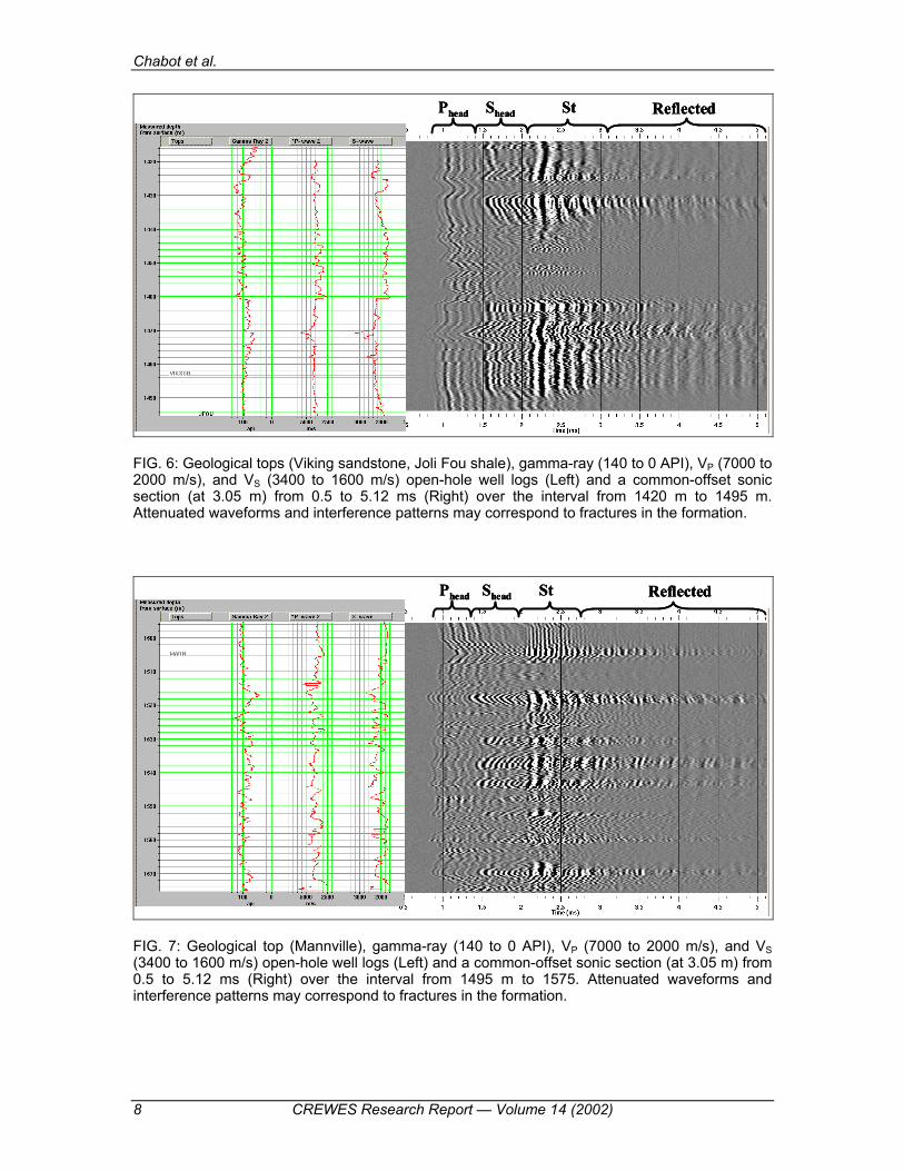
analyzing the raw full-waveform data in a single-receiver constant offset (at 3.05 m) variable-density plot or a common-offset sonic section (Figures 6, 7, 8 and 9). The analysis of the attenuation and interference patterns in the waveforms in the common-offset sonic section provides an indication of the presence or absence of fractures and their orientations (Morris et al., 1964). In the common-offset sonic section shown in Figure 8 it can be noted that the shear and the Stoneley waves energy are attenuated in the vicinity of the three coal seams but not the compressional waves. This may be indicative of the angle of inclination (90 to 60° with respect to the borehole axis) of the attenuating zones (in this case the three coal seams). The window to identify reflections in the raw waveforms is located, in time, after the Stoneley arrivals (Figures 6 to 9). However, there are no obvious reflections at this stage.

A 40-m section of the full-waveform dataset (Figure 8), which corresponds to 267 shot records, was selected. This section covers a segment of the borehole from a measured depth of 1580 m to 1620 m and intersects, at an angle of approximately 65°, three known coal seams. These coal seams are stringer seams and have an average density of 1800 kg/m3, an average compressional velocity of 3000 m/s, and an average shear velocity of 1800 m/s. They are surrounded by shaly formations with an average density of 2600 kg/m3, an average compressional velocity of 4000 m/s and an average shear velocity of 2400 m/s.

Chabot et al.


Phead Shead St ReflectedPhead Shead St ReflectedPhead Shead St Reflected

FIG. 6: Geological tops (Viking sandstone, Joli Fou shale), gamma-ray (140 to 0 API), VP (7000 to 2000 m/s), and VS (3400 to 1600 m/s) open-hole well logs (Left) and a common-offset sonic section (at 3.05 m) from 0.5 to 5.12 ms (Right) over the interval from 1420 m to 1495 m. Attenuated waveforms and interference patterns may correspond to fractures in the formation.


FIG. 7: Geological top (Mannville), gamma-ray (140 to 0 API), VP (7000 to 2000 m/s), and VS (3400 to 1600 m/s) open-hole well logs (Left) and a common-offset sonic section (at 3.05 m) from 0.5 to 5.12 ms (Right) over the interval from 1495 m to 1575. Attenuated waveforms and interference patterns may correspond to fractures in the formation.

Single-well imaging



FIG. 8: Geological tops (coal seams), gamma-ray (140 to 0 API), VP (7000 to 2000 m/s), and VS (3400 to 1600 m/s) open-hole well logs (Left) and a common-offset sonic section (at 3.05 m) from 0.5 to 5.12 ms (Right) over the interval from 1575 m to 1655 m. Attenuated waveforms and interference patterns may correspond to fractures in the formation.


FIG. 9: Geological tops (Glauconitic sandstone, Ellerslie sandstone, Pekisko limestone), gamma-ray (140 to 0 API), VP (7000 to 2000 m/s) and VS (3400 to 1600 m/s) open-hole well logs (Left) and common-offset sonic section (at 3.05 m) from 0.5 to 5.12 ms (Right) over the interval from 1655 m to 1730. Attenuated waveforms and interference patterns may correspond to fractures in the formation.

Chabot et al.


Composite sonic image The waveform processing and imaging of the 40-m section of field data was done with

the help of the flow described by Chabot et al. (2001) with improvements. The problem with full-waveform data acquired with a conventional well-logging tool, in contrast to full-waveform data acquired with a research tool (see Table 1), is the fact that we have spatial aliasing and a limited number of offsets and traces per shot record. To address these problems, radial trace filtering (Henley, 1999) and the equivalent-offset method of prestack migration (Bancroft et al., 1998) were used in our processing flow.

In this work, an improved geometry assignment allowed us to incorporate all the recorded full-waveform traces in the overall processing flow. Also, this improved geometry assignment had the impact of generating a more regular fold pattern.

Added to the original processing flow was an attempt to apply refraction statics to the full-waveform dataset. After picking first breaks, we attempted the application of refraction statics on the full-waveform dataset with the help of Hampson-Russell�s GLI3D� software. However, the unsuitability of the output (time to nearest milliseconds and distance to nearest metres) limited its usefulness. Improvements in the precision of the output are being provided with the upcoming version 5.0.7 of GLI3D� software.

The attenuation and removal of the S headwave (pseudo-Rayleigh) and Stoneley waves from individual shot records was done with a series of more efficient radial dip filters (Henley, 1999). In addition, the reflected Stoneley arrivals, with negative velocities, were also filtered out of the shot records, when present, using an additional radial dip filter. Radial dip filters have the advantage of focusing on localized events in the x-t domain rather than widespread families of events (e.g. f-k filters) and successive radial trace filters can be applied to the x-t domain.

Better trace balancing was applied in order to achieve about the same amplitudes at all times of the traces. Also, an appropriate trace mute was applied to remove any road noise from the tool arriving before the first arrivals.

The equivalent-offset method (EOM) of prestack time migration (Bancroft et al., 1998) was applied using parameters appropriate for a borehole environment. In this case, improvements include the formation of two-sided equivalent-offset (EO) gathers [formally known as common-scatter-point (CSP) gathers] with a more appropriate equivalent-offset parameter and the use of a better velocity model for the application of normal-moveout (NMO) correction before stacking. The advantages of this method are: the EO gather has higher fold and larger offset range than the common-midpoint (CMP) gather. Also, the EO gather is composed of all input traces within the prestack migration aperture and the creation of EO gathers is fast because no time-shifting, scaling, or filtering is involved. Finally, the EOM has been successfully used to image vertical array data (Bancroft and Xu, 1999).

Two-sided EO gathers (one set of EO gathers consist of gathers with only positive equivalent offsets, while the other has only negative equivalent offsets) were formed for a positive and a negative value of 10 m for the equivalent offset distance. Also, a velocity of 3500 m/s was selected for the migration aperture. These values were selected because no steep dips were expected in the subsurface. For an improved resolution, the

Single-well imaging


equivalent-offset bin size was selected at 0.075 m. Two-sided EO gathers have the advantage of making it possible to see how the contributions from different azimuths differ from each other and thus linear, diffracted, and dipping events can be better distinguished.

The following steps, as presented by Chabot et al. (2001), have remained unchanged and are displayed graphically in Figure 10. The two-sided EO gathers were split into two separate families of gathers. The EO gathers with negative offsets, looking downhole, were sorted together representing the updip portion of the borehole, while those with positive offsets, looking uphole, were sorted together representing the downdip portion of the reflector in relation to the borehole. Once this separation was completed, we applied NMO with the correct velocities to the EO gathers representing the updip portion of the hole, followed by a conventional stack, thus creating the prestack time-migration image of the updip region of the hole. We also applied NMO with the same velocities to the family of EO gathers representing the downdip portion of the hole, followed by a conventional stack, thus creating the prestack time-migration image of the downdip region of the hole.

Because we are interested in the reflected P arrivals in order to form an image of structural changes away from the borehole, the application of the NMO correction used the compressional velocity profile as acquired by the well-logging tool. The two processed sections are next combined along their common zero time, which in the final image becomes the well axis. The final processing results are presented in a composite sonic image in Figure 11.

Geometry

Filtering

EO gathers

NMO

Straight Stack

EO gathers sorting

NMO

Straight Stack

Composite sonic image

updi

p

dow

ndip

(Static corrections)

Common-offset sonic section

Geometry

Filtering

EO gathers

NMO

Straight Stack

EO gathers sorting

NMO

Straight Stack

Composite sonic image

updi

p

dow

ndip

(Static corrections)

Common-offset sonic section

FIG. 10: Schematic diagram representing the proposed processing flow used to transform raw full-waveform data acquired by the acoustic well-logging tool into a composite sonic image.

Chabot et al.


Downdip Updip

Bor

ehol

e ax

is (4

0 m

) �flu

id-fi

lled

Coal 1

Coal 2

Coal 3

5.12 ms5.12 ms

Downdip Updip

Bor

ehol

e ax

is (4

0 m

) �flu

id-fi

lled

Coal 1

Coal 2

Coal 3

5.12 ms5.12 ms

Downdip Updip

Bor

ehol

e ax

is (4

0 m

) �flu

id-fi

lled

Coal 1

Coal 2

Coal 3

5.12 ms5.12 ms

FIG. 11: Prestack time-migration image of the full-waveform data (left) and computed impedance and reflectivity from open-hole well logs (right). This composite sonic image represents a cross-sectional view of the three coal seams intersecting the borehole. The borehole interval shown here is 40 m in length. The lateral extent of investigation, away from either side of the borehole wall, is 5.12 ms. On this image, the colours of blue, white and red represent negative, zero and positive amplitudes respectively. Vertical to horizontal scale of the composite sonic image is 1:1 (approximately). Arrows point out possible reflections.

COMPARISON WITH SURFACE SEISMIC DATA To explore the resolution gap, the composite sonic image in Figure 11 was compared

with a seismic section that intersects the borehole along its dip direction (Figure 12). This vertical-component seismic section was extracted from a 3C-3D surface-seismic volume acquired over the Blackfoot field in 1995. The seismic data have a 30-m bin size, a CDP

Single-well imaging


fold of 10 to 170 Hz and a final bandwidth of 10-80 Hz. In comparing the composite sonic image from Figure 11 with the seismic section in Figure 12, the factors of scale and resolution become apparent. The three coal seams, associated with zero-amplitude crossings in the seismic section (Figure 12), hardly have the same amplitude characteristics in the composite sonic image.

FIG. 12: Seismic section (vertical component) intersecting the deviated borehole along its dip direction. The time scale of the seismic section is from 700 ms to 1120 ms. The surface position of the well is represented by the solid dot. The synthetic seismogram incorporating the well-log information is located in its true vertical position underneath the solid dot. The 40-m borehole segment on the right-hand side of the figure indicates the corresponding interval here and in Figure 11.

DISCUSSION The proposed processing flow has been tested on full-waveform sonic data. The

composite sonic image shown in Figure 11 looks promising, with possible reflections. However, the image has difficulty showing the reflection from the expected three dipping coal seams intersecting the borehole at an angle. This is probably caused by the fractured coal units attenuating the energy source of the well-logging tool as it crosses the coals. In addition, incompletely cancelled noise modes, weak reflecting boundaries, and the large angle (~65°) between the borehole and the geological interfaces are causing weakness in the reflections.

To locate the sonic image in its proper azimuthal orientation, additional well data, such as dipmeter information, is required. In other words, results from single-well imaging need to be interpreted in conjunction with other borehole data. It is important to note that this method cannot resolve an image in geologically complex reservoirs.

This processing flow holds promise for application to other field data.

Chabot et al.


FUTURE WORK The sonic-waveform processing and imaging flow presented in this paper need to be

improved further. This could be achieved by the addition of new steps in the processing flow such as: dereverberation with predictive deconvolution, the selection of a proper migration datum, and the use of the borehole calliper data to help in the application of elevation statics to the full-waveform data. Finally, the improved processing flow could best be tested on full-waveform data acquired in deviated wells intersecting beds at angles of 35° or less between the wellbore and the interface.

ACKNOWLEDGEMENTS We would like to thank K. Hall and H. Bland for their assistance in this work, the

sponsors of CREWES for their financial support, and EnCana Corporation Ltd. and Schlumberger Ltd. for providing us with the field dataset.

REFERENCES Bancroft, J.C., Geiger, H.D., and Margrave, G.F., 1998, The equivalent offset method of prestack time

migration: Geophysics, 63, 2042 - 2053. Bancroft, J.C. and Xu, Y., 1999, Equivalent offset migration for vertical receiver arrays: 69th Ann. Internat.

Mtg., SEG, Expanded Abstracts, 1374-1377. Chabot, L., Henley, D.C., Brown, R.J., and Bancroft, J.C., 2001 Single-well seismic imaging using the full

waveform of an acoustic sonic: CREWES Research Report, 13, 38-1. Cheng, N., Cheng, C.H., and Toksöz, M.N., 1995, Borehole wave propagation in three-dimensions: Journal

of the Acoustical Society of America, 97, 3483-3493. Coates, R., Kane, M., Chang, C., Esmersoy, C., Fukuhara, M., and Yamamoto, H., 2000, Single-well sonic

imaging: High-definition reservoir cross-sections from horizontal wells: SPE 65457. Fortin, J.P., Rehbinder, N., and Staron, P., 1991, Reflection imaging around a well with the EVA full-

waveform tool: Log Analyst, May-June, 271-278. Harrison, A.R., Randall, C.J., Aron, J.B., Morris, C.F., Wignall, A.H., Dworak, R.A., Rutledge, L.L., and

Perkins, J.L., 1990, Acquisition and analysis of sonic waveforms from a borehole monopole and dipole source for the determination of compressional and shear speeds and their relation to rock mechanical properties and surface seismic data: SPE 20557.

Henley, D.C., 1999, The radial trace transform: an effective domain for coherent noise attenuation and wavefield separation: 69th Ann. Internat. Mtg., SEG, Expanded Abstracts, 1204-1207.

Hornby, B.E., 1989, Imaging of near-borehole structure using full-waveform sonic data: Geophysics, 54, 747-757.

Liu, Q.-H., Schoen, E., Daube, F., Randall, C., Liu, H.-L., and Lee, P., 1996, A three-dimensional finite difference simulation of sonic logging: Journal of the Acoustical Society of America, 100, 72-79.

Miller, S., Aydemir, E.Ö., and Margrave G.F., 1995, Preliminary interpretation of P-P and P-S seismic data from the Blackfoot broad-band survey: CREWES Research Report, 7, 42-1.

Morris, R.L., Grine, D.R., and Arkfeld, T.E., 1964, Using compressional and shear wave acoustic amplitudes for the location of fractures: Journal of Petroleum Technology, 623-632

Paillet, F.L. and Cheng, C.H., 1991, Acoustic waves in boreholes: CRC Press, 264 pages. Schlumberger, 1997, DSI� � Dipole Shear Sonic Imager: Corporate brochure SMP-9200, 36 pages.

single-well imaging using full waveform sonic data - · pdf filesingle-well imaging using full...

Documents