1

Supporting Information of the paper

Single-molecule derivation of salt dependent base-pair

free energies in DNA

by

Josep M. Hugueta, Cristiano V. Bizarroa,b , Núria Fornsa,b, Steven B. Smithc, Carlos

Bustamantec,d, Felix Ritorta,b,1

aDepartament de Física Fonamental, Universitat de Barcelona, Diagonal 647, 08028 Barcelona, Spain. bCIBER-BBN de Bioingenieria, Biomateriales y Nanomedicina, Instituto de Sanidad Carlos III, Madrid,

Spain. cDepartment of Physics, dDepartment of Molecular and Cell Biology and Howard Hughes Medical

Institute, University of California, Berkeley, CA 94720.

1 To whom Correspondence should be addressed. Facultat de Física, UB Diagonal 647, 08028 Barcelona, Spain Phone: +34-934035869 Fax: +34-934021149 E-mail: fritort@gmail.com, ritort@ffn.ub.es

2

Contents

S1. Optical Tweezers instrument 3

S2. Force and distance calibration 4

S3. DNA molecular constructs 8

S4. Synthesis of ssDNA 9

S5. Elastic parameters of ssDNA and comparison between the models 9

S6. Monte Carlo minimization algorithm 11

S7. Drift and shift function 12

S8. Calculation of melting temperatures 16

S9. Enthalpy and entropy inference 17

S10. Free energy of the loop 20

S11. Sampling of energy states distribution 20

S12. Thermodynamics of DNA unzipping 22

S13. Dependence of the optimization algorithm on the initial conditions 23

S14. Errors in the Monte Carlo optimization 23

References 26

Figures 27

Tables 46

3

S1. Optical Tweezers instrument

The experimental setup (see Figure S2) consists of two counter-propagating laser beams of

845 nm wavelength that form a single optical trap where particles can be trapped by

gradient forces. The setup is similar to the one described by Smith et al. (1). Here two

microscope objectives with numerical aperture 1.20 act as focusers and condensers

simultaneously. One laser beam is focused through its objective while the other objective

collects the exiting light, which is redirected to a position-sensitive detector (PSD). The

laser beams have orthogonal polarizations thus making their optical paths separable by

using polarized beamsplitters. When the optical trap exerts a force on a particle, the

unbalanced exiting light is redirected from the back focal plane of the objective to a PSD

that returns a current proportional to the force. Since the force is measured using

conservation of light momentum, the calibration does not depend on the power of the

lasers, the refraction index of the microspheres, their size or shape, the viscosity or

refractive index of the buffer.

The optical trap can be positioned with the so-called wigglers. A wiggler is a device that

bends the optical fiber of the laser using two piezoelectric crystals that mechanically push

the fiber in such a way that the light is redirected to the desired position. There are two

piezos per laser to place the optical trap at the desired location in the XY plane. The

position of the center of the trap is measured by separating 5% of the light from the laser

beam with a pellicle beam-splitter and forming a light-lever. For the lightlever we use a

PSD in such a way that the measured current is proportional to the position of the beam.

See refs. 2 and 3 for further information.

All the currents measured by the PSDs are processed by electronic microprocessors and the

data are sent to a computer and converted to forces and distances. The acquisition

frequency is 1 kHz and the resolution is 0.1 pN in force and 0.5 nm in distance. The

experiments are carried out in a fluidics chamber that holds the micropipette. The whole

chamber can be moved with a motorized stage. The instrument and the surrounding room

are kept at a constant temperature of 25 ± 0.3 ºC.

4

S2. Force and distance calibration

According to the experimental setup (Sec. S1), the instrument detects the change in the

light momentum of the laser beams that form the optical trap, which allows us to directly

measure the force accurately. There is a linear relation between the PSD reading and the

actual force exerted on the bead by the optical trap:

oyy FPSDMF +!= [1]

where Fy is the actual force on the y-axis in pN, PSDy is the sum of the readings of the

PSDs of both traps in the y direction in adu (analog to digital units), M is the calibration

factor and Fo is an offset, already corrected by the data acquisition board. The process of

calibration consists on accurately find out the value of M, which is independent of the trap

power. Here we only show the method used in force calibration for the y-axis. The same

procedure applies to x and z axis. Three different methods were used to calibrate the PSD

that measures the force.

In the first method, we collected 30 s of Brownian PSDy signal for a trapped microsphere in

distilled water at low laser power (Figure S3a), in order to have a low corner frequency.

The signal was squared and a power spectrum built up (Figure S3b) by averaging the

spectra of 1.00-second windowed frames of the data. The averaged spectrum was fit in log-

log scale (Figure S3c) to a Lorentzian profile:

!

SPSDy(") = PSDy (" ) # PSDy

*(" ) =

A

B + (2$" )2 [2]

where

!

SPSDy(") is the power density of the PSDy noise in adu units and A and B are the fit

parameters. The power density of the force noise of a trapped particle (1) is expected to

follow a Lorentzian distribution according to:

5

!

SFy (") = Fy (") # Fy*(" ) =

2k kBT $c

$c

2+ (2%" )

2 ; $

c=k

& [3]

where

!

SFy (") is the force power density of the y-axis force, k is the trap stiffness in the y

direction, kB is the Boltzmann constant, T is the temperature, ωc is the corner frequency and

γ is the drag coefficient of the bead in distilled water. The drag coefficient for spherical

particles at low Reynolds number regime can be calculated according to γ=6πηR, where η

is the viscosity of distilled water at 25ºC and R is the bead radius. The viscosity of water at

25ºC is taken as η=8.9·10-4 Pa·s and the diameter of the bead is taken as R=3.00±0.05 µm

from scanning electron microscopy measurements (average over 100 3.0-3.4 µm

polystyrene beads from Spherotech, Libertyville, IL). Using Eq. 1, the measured power

spectrum (in adu units) and the expected one (in pN) can be related:

!

SFy (") = M2# SPSDy

(" )

2k kBT $c

$c

2+ (2%" )

2=

M2A

B + (2%" )2

[4]

from which the calibration factor (M) and the trap stiffness (k) can be obtained by

identifying the parameters of the fit spectrum with the expected one:

!

2k kBT "

c= M

2A

"c

2= B

# $ %

M = 2 k

BT & B /A

k = & B

# $ '

% ' [5]

The two force calibration factors extracted from the power spectra measured at two

different laser powers differed less than 1%. The stiffness of the weak trap was

k=3.22±0.05 pN/µm, while k=6.20±0.07 pN/µm for the stronger trap. A first check of the

correctness of these numbers was made by calculating the trap stiffness from the force

fluctuations (i.e. the PSD reading) of previous measured time series (Figure S3a). The

fluctuation-dissipation relation for a trapped particle can be written as:

6

!

Fy2

= k " kBT [6]

where

!

Fy2 is the variance of the y force. Since we have already calculated the calibration

factor (M) we can combine Eq. 6 and 1 to write:

Tk

PSDMk

B

y

22

= [7]

where

!

PSDy

2 is the variance of the PSD in the y direction. In this way we can calculate the

trap stiffness without knowing the viscosity of water. The values obtained were

k = 3.26 pN/nm for the soft trap and k = 6.15 pN/nm for the stiff trap, which represents an

error of 1.5%. Once the optical trap was calibrated, a check was performed to measure the

stiffness using another independent method (Figure S3d) which does not use the force

noise. A bead was stuck at the tip of the micropipette. The optical trap was aligned in the

center of the bead and short displacements of the optical trap were performed while

recording the force vs. trap displacement and keeping the micropipette at fixed position.

The slope of the linear region of this curve is the trap stiffness. The values of the stiffness

obtained were k = 3.200±0.002 pN/µm for the soft trap and k = 6.28±0.02 pN/µm for the

stiff trap. These values differ by less than 1.5% with respect to the power spectrum method.

In the second method, the PSDs were calibrated using Stokes law (Figure S3e). A

microsphere was trapped and the whole fluidics chamber moved at a fixed speed using the

motorized stage. The microsphere undergoes a force produced by the surrounding fluid

which is proportional to the speed. Knowing the microsphere radius and the viscosity of

distilled water, the relation between the PSDs readings and the velocity of the fluid gives

the calibration factor. The calibration factor is obtained from averaging 40 different beads

(same beads as above). The calibration factor obtained agreed within 2% with the previous

methods.

A third method that does not depend on the bead size and viscosity of water was used to

check our previous calibration protocols. A similar setup to Figure S2 (instrument in

7

Barcelona) was also made in Berkeley and calibrated using the known momentum

properties of light. It can be shown (1) that the force sensitivity of the PSD detector is

given by

!

M = (RD / fO ) /("# c) [8]

where RD is the half-width of the PSD chip, fo is the objective lens focal length, Ψ is the

power sensitivity of the PSD (signal/watts referenced to the trap position) and c is the speed

of light. The PSD responsivity was measured with an optical power meter (Thorlabs PM30-

130) and PSD dimensions were tested by using a test laser on a motorized stage (4). Using

this calibration, we pulled the same 2.2 kb molecule in Berkeley and obtained the data

shown in Figure S4 where we see good agreement between the FEC of the 2.2 kb molecule

measured in different instruments. The mean unzipping force differs by less than 0.15 pN.

The calibration of the lightlever position sensor is done using the motors that move the

XYZ-stage. The Thorlabs Z-606 motors have a shaft encoder that counts the turns of the

axes so that the position of the stage can be determined. A trapped microsphere is held

fixed at the tip of the micropipette and the optical trap follows the position of the

microsphere by keeping the total force equal to zero using a force feedback mechanism

(Figure S5a). When the micropipette moves, the wiggler acts to reposition the center of the

trap in order to follow the bead. The calibration factor for the position can be determined

through the relation between the reading of the position PSDs (also known as lightlevers)

and the position of the motor. This calibration protocol provides slightly different

calibration factors (less than 3% difference) depending on the direction in which the motor

is moving, due to the backslash of the motor (Figure S5b,c).

Summing up, we verified that our instrument is well calibrated in force within 0.5 pN (i.e.

~3%) and in distance within 3%.

8

S3. DNA molecular constructs

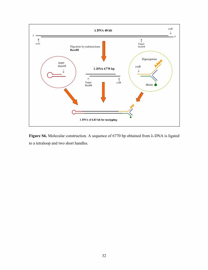
A 6770 bp insert DNA was isolated by gel extraction of a BamHI digestion of λ phage

DNA (see Figure S6). Two short handles of 29 bps and one tetraloop (5’-ACTA-3’) were

ligated to the insert that has the λ cosR end and a BamHI sticky end. To construct the DNA

handles, an oligonucleotide (previously modified at its 3’ end with several digoxigenins

using DIG Oligonucleotide Tailing Kit, 2nd Generation, Roche Applied Science) was

hybridized with a second 5’ biotin-modified oligonucleotide giving a DNA construction

with one cohesive end complementary to cosR and two 29 nucleotide long ssDNA at the

other end. These two ssDNA have the same sequence and they were hybridized with a third

oligonucleotide, which is complementary to them, resulting in two dsDNA handles. This

construction was attached to the insert DNA by a ligation reaction. A fourth self-

complementary oligonucleotide, which forms a loop in one extreme and a cohesive BamHI

end at the other, was ligated to the BamHI sticky end of the insert DNA. The DNA was

kept in aqueous buffer containing 10 mM Tris-HCl (pH 7.5) and 1 mM EDTA.

Streptavidin-coated polystyrene microspheres (2.0-2.9 µm; G. Kisker GbR, Products for

Biotechnologie) and protein G microspheres (3.0-3.4 µm; Spherotech, Libertyville, IL)

coated with anti-digoxigenin polyclonal antibodies (Roche Applied Science) were used for

specific attachments to the DNA molecular construction described above. Attachment to

the anti-digoxigenin microspheres was achieved first by incubating the beads with tether

DNA. The second attachment was achieved in the fluidics chamber and was accomplished

by bringing a trapped anti-digoxigenin and a streptavidin microsphere close to each other.

The 2.2 kb construct was obtained taking the 2215 bp fragment from a SphI digestion of λ

DNA. The same two short handles and tetraloop used for the 6.8 kb DNA are used for the

2.2 kb construct, with the following exceptions: the two handles are hybridized to the

2215 bp DNA through the cosL cohesive end of λ DNA, and the tetraloop was added to the

insert DNA using the SphI sticky end. Table S3 shows the fraction of the 10 NNBPs found

along the two sequences.

9

S4. Synthesis of ssDNA

A 3 kb ssDNA molecular construct was obtained by pH denaturation (strand separation) of

a 3 kb dsDNA (see Figure S7). The dsDNA was obtained from PCR amplification of a

~3 kb fragment of λ-DNA. One of the primers used in the process was already labeled with

Biotin. The resulting product was cleaved with the endonuclease XbaI producing a cohesive

end. Another 24 base oligonucleotide (previously labeled with several digoxigenins at its 3’

end by using terminal transferase) was hybridized with a second 20-base long

oligonucleotide giving a DNA construction with one cohesive end complementary to XbaI.

Both products were annealed and ligated resulting in one 3 kb dsDNA molecule. To

produce ssDNA, the molecular construct was incubated with Streptavidin coated beads for

30 min at room temperature in a volume of 15 µl of 10 mM NaCl TE buffer. Afterwards,

35 µl of 0.1 M NaOH were added in order to cause the separation (i.e. denaturation) of the

strands. After 30 min, the sample was centrifuged. The white precipitate of beads and

ssDNA was re-suspended in TE buffer. The second attachment with the antidigoxigenin

beads was achieved in the fluidics chamber with the help of the micropipette.

S5. Elastic parameters of ssDNA and comparison between the

two models

From the pulling experiments on ssDNA (see Fig. 2e in main text and Figure S8) we

conclude that the Worm-Like Chain (WLC) model correctly describes the elastic response

of the ssDNA at low salt concentration (<100 mM [NaCl]) whereas the Freely-Jointed

Chain (FJC) model works better at higher salt concentrations (>100 mM [NaCl]). Strictly

speaking, in the later regime both models fail because the elastic response of the ssDNA

exhibits a force plateau at low forces (Fig. 1e in main text or rightmost panel in Figure S8).

Such force plateau indicates that the ssDNA has some structure at high salt concentration

and low forces. The shape of the force plateau is hardly reproducible and varies from

pulling to pulling and from molecule to molecule. Therefore, it is quite difficult to establish

10

which is the native state of a ssDNA molecule at low forces. Nevertheless, our goal is to

measure the free energy difference between two complementary ideal ssDNA chains and

the duplex of dsDNA that they form. So we do not need to know the elastic response of a

self-interacting ssDNA molecule. Instead, we assume that the ssDNA behaves like an ideal

chain.

In order to obtain the elastic response of the ssDNA, we have to fit the stretching

experimental data of the 3 kbp ssDNA molecules to the appropriate model (FJC or WLC

depending on the salt concentration). At high salt concentration, any pulling FDC of a

ssDNA molecule (like in Fig. 1e main text) will be correctly fit by a FJC model above

15 pN because no secondary structure will survive at this force. Therefore, we can fit the

FDCs above 15 pN to a FJC model. Note that we are clearly neglecting any possible

secondary structure that can be formed below 15 pN, because the FJC model itself is an

ideal chain and it does not account for such structures. Figure S8 shows the elastic response

of the ssDNA for three different salt conditions together with the best fits to the two elastic

models (WLC and FJC). Table S4 summarizes our results for the elastic parameters.

The fit is performed as follows. The measured FDCs of the ssDNA (right panels Fig. 2e

main text and Figure S8) are converted to a force-extension curve (FEC) after subtracting

the contribution of the optical trap according to,

!

xs = xtot"f

k

where xs is the extension of the ssDNA, xtot is the total distance, f is the force and k is the

stiffness of the optical trap. The resulting FEC is fit to a FJC or a WLC (see upper panels in

Figure S9). The fitting parameters are the Kuhn length (b) or the persistence length (lp)

depending on the model, and the interphosphate distance (d). The FEC is forced to pass

through the point (xs=0, f =0), while the number of bases is fixed to n=3000 (see “Synthesis

of ssDNA” in Materials and Methods section in main text).

As a final test, the fit Kuhn length (or persistence length) of the ssDNA is introduced into

the equation of the total distance of the system (see “Calculation of the equilibrium FDC”

11

in the Materials and Methods section in main text). When the molecular construct is fully

unzipped, it is actually a ssDNA molecule tethered between two beads (plus two short

dsDNA handles). So the last part of the unzipping FDC (above ≅15 pN) is giving us the

elastic response of the ssDNA. Here, the ssDNA shows its elastic response because no

secondary structure can be formed. Lower pannels in Figure S9 show that the last part of

the unzipping FDCs are correctly described by a ssDNA molecule of 2×6838 bases.

In the end, we have fit the elastic response of the ssDNA to a FJC above 15 pN. Below this

force, we have assumed that the FJC correctly describes the ideal elastic response of the

ssDNA, i.e. in the absence of secondary structure.

S6. Monte Carlo minimization algorithm

We developed an algorithm based on Monte Carlo (MC) minimization where we start from

an initial guess for the energies εi (i=1,..,10) and do a random walk in the space of

parameters in order to minimize the error function (Eq. 2 main text). The method is just a

standard Simulated Annealing optimization algorithm (5) adapted to our particular problem

that speeds up considerably the time to find the minimum as compared to standard Steepest

Descent algorithms. The error landscape defined by Eq. 2 main text is not rough and there

is no necessity to use a MC algorithm. Nevertheless, we find that the MC optimization is

computationally more efficient (i.e. faster) than other optimization algorithms (such as

Steepest Descent) because no derivatives need to be calculated. A fictive temperature is

defined to control how the space of parameters is explored. Each new proposal is accepted

or rejected using a Metropolis algorithm. According to the Metropolis algorithm a move is

always accepted if ΔE < 0 (where ΔE is the change in the error after the proposal). If

ΔE > 0, a random number r from a standard uniform distribution

!

r "U(0,1) is generated

and the move accepted if

!

e"#E /T

> r and rejected if

!

e"#E /T

< r . A quenching MC protocol,

where the minimization algorithm is run at a very low fictive temperature, was found to be

particularly efficient.

12

We start from the unified values for the NNBP energies to enforce the system to explore the

basin of attraction in the vicinity of the unified values. The system is allowed to evolve

until the total error reaches a minimum. This method is essentially a steepest descent

algorithm with the advantage that the free energy derivatives need not be calculated (see

Figure S10a). Once the system has found the minimum, we start another MC search to

explore other solutions in the vicinity of the minimum. For that we use a heat-quench

algorithm (see Figure S10b) in which the system is heated up to a large fictive temperature

until the error is 50% higher than the error of the first minimum. Afterwards, the system is

quenched until the acceptance of MC steps is lower than 0.03%. This procedure is repeated

many times until the multiple solutions allow us to estimate the error of the algorithm. The

possible values for the stacking energies are Gaussian distributed in a region of width

approximately equal to 0.05 kcal/mol calculated (see Figure S10c). The analysis revealed

that the optimization algorithm is robust and leads to the same solution when the initial

conditions are modified (see Sec. S13). Different molecules and different sequences

converge to energy values that are clustered around the same value (see Sec. S14).

S7. Drift and shift function

Instrument drift is a major problem in single molecule experiments. The drift is a low

frequency systematic deviation of measurements due to macroscopic effects. The

importance of drift depends on the kind of the experiment and the protocol used. Our

unzipping experiments are performed at very low pulling speeds (typically around

10 nm/s), so measuring a whole unzipping/rezipping FDC may take 10 minutes or longer.

Therefore it is useful to model drift in order to remove its effects and extract accurate

estimates for the NNBP energies.

Our experimental measurements are force versus trap position as measured by the

lightlevers (Sec. S1). The unzipping/zipping curves contain reproducible and recognizable

landmarks (i.e. slopes and rips) which indicate the true position of the trap. Therefore we

devised a way to take advantage of these landmarks to correct for the instrumental drift.

13

Correction for drift is introduced in terms of a shift function s(xtot) which is built in several

steps. Due to its relevance for data analysis we describe the steps in some detail:

Step 1. We start with the experimental FDC filtered at 1 Hz bandwidth and fix the origin of

coordinates for the distance xtot (trap distances are relative) by fitting the last part of the

experimental FDC (black and magenta curves in Figure S11a) corresponding to the

stretching of the ssDNA when the hairpin is fully unzipped.

Step 2. Having fixed the origin of coordinates we calculate the predicted FDC by using the

Unified Oligonucleotide (UO) NNBP energies. It is shown in red (Figure S11a, S11b). The

qualitative behavior is acceptable (all force rips are reproduced). However, the predicted

mean unzipping force is higher than the value found experimentally and the force rips are

not located at the correct position.

Step 3. Next we generate a FDC with NNBP energies lower than the UO energies until the

mean unzipping forces of the predicted and the experimental FDC coincide. Typically what

we do is multiplying all the 10 NNBP UO energies by a factor ~0.95. The new NNBP

energies have an absolute value 8-10% lower than the UO NNBP energies. The resulting

FDC with these new energies is shown in green in Figure S11b (in this particular case we

took

!

"i

New= 0.92 # "

i

Mfold ). Although the mean unzipping force of the green and black curves

is nearly the same, there is misalignment between the rips along the distance axis.

Moreover, there are discrepancies between the predicted and measured heights of the force

rips. As we will see below, the shift function will correct the horizontal misalignments and

the NNBP energies will correct the discrepancies along the force axis.

Step 4. We now introduce a shift function that uses the slopes preceding the rips as

landmark points to locally correct the distance to align the experimental data with the

theoretical prediction. First, we want to know the approximate shape of the shift function

and latter we will refine it. This is done by looking for some characteristic slopes of the

sawtooth pattern along the FDC and measuring the local shift that would make the two

slopes (theoretical and experimental) superimpose. Figure S11c shows zoomed regions of

14

the FDC and the blue arrows indicate the local shift that should be introduced in each slope

to correct the FDC. The orange dots shown in the upper panel of Figure S11d depict the

local shifts vs. the relative distance that have been obtained for the landmark points. These

orange dots represent a discrete sampled version of an ideal shift function that would

superimpose the predicted and the experimental FDC. Because these dots are not

equidistant, we use cubic splines to interpolate a continuous curve every three landmark

points. The resulting interpolated function that describes the local shift for any relative

distance is shown in violet. Note that the violet curve passes through all the orange dots.

Step 5. Starting from the cubic splines interpolation of the shift function that we have found

(violet curve in upper panel Figure S11d) we can define new equidistant points (yellow dots

in lower panel Figure S11d) that define the same shift function. The yellow equidistant

points are separated 100 nm. We call these yellow points “Control points”.

Step 6. We now introduce the shift function into the calculation of the theoretical FDC. The

results are shown in Figure S11e. Again, the black curve is the experimental FDC, the

green curve is the predicted FDC without the local shift correction and the magenta curve is

the predicted FDC with the local shift function obtained previously. Note that the magenta

and green curves are identical, except for local contractions and dilatations of the magenta

curve. The slopes of the magenta and the black curves now coincide. Still, the NNBP

energies must be fit to make the height of the rips between the theoretical and experimental

curve coincident.

Step 7. At this point we start the Monte Carlo fitting algorithm. At each Monte Carlo step

we propose new values for the 10 NNBP energies and we also adjust the shift function in

order to superimpose the theoretical and experimentally measured FDCs. The shift function

is adjusted by modifying the values of the control points (yellow dots in lower panel of

Figure S11d). The horizontal position of the yellow points is always the same (e.g. the

yellow dot located at Relative Distance = -1000 nm will always be located there). What we

change when we adjust the shift function is the value of each point (e.g. the yellow dot

located at Relative Distance = -1000 nm may change its shift value from -54 to -20 nm).

15

During the Monte Carlo optimizing procedure the shift function modifies its shape as the

NNBP energies are modified. The results are shown in Figure S11f. Black curves show

snapshots of the evolution of the shift function during the optimization process from the

initial shape (red curve). The green curve shows the final shift function (the control points

are not depicted in Figure S11f, only the interpolated shift function). When we finally

calculate the theoretical FDC using the optimal shift function and the optimal NNBP

energies we get the maximum overlap between the theoretical prediction and the

experimental FDC. Black curve in upper panel in Figure S11g is the experimental FDC and

red curve is the predicted FDC after having fit the NNBP energies and the shift function.

The correction for drift has now finished. The optimal shift function is also shown in the

lower panel in Figure S11g.

All the steps we described before were applied to all different molecules and salt conditions

we measured. Measurements from different molecules have shift functions of similar

shapes (Figure S12). We have checked that the undulations are not an artifact of the spline

interpolation. The undulations remain when the number of control points of the shift

function is increased. The net shift observed in some curves (around ±100 nm) might be

explained by improper calibration of the distance (around 4%). The undulations observed in

the shift function might be due to non-linearities in the lightlever (i.e. trap position)

measurements or interference fringes in the lenses and the pellicle located along the optical

path to the PSDs. The undulations in the shift function might also be correlated with the

DNA sequence as emerges from the fact that undulations observed in different molecules of

the same sequence appear at nearby positions. This might indicate new effects in the

unzipping curves not accounted for in the NN model (e.g. the presence of next nearest

neighbor corrections).

We have also checked whether the correction introduced by the shift function also could be

explained by a dependence of the Kuhn length on the contour length. To our knowledge,

such dependence has not ever been reported. Yet it is interesting to evaluate the

consequences of such hypothetic dependence. By letting the Kuhn length depend on the

number of open base pairs, the position of the theoretical and experimental slopes and rips

match each other if the Kuhn length increases as the contour length decreases. However

16

this matching occurs at the price of an increasing average mean unzipping force as the

molecule unzips and the ssDNA is released, an effect which is not experimentally observed.

We conclude that the shift function is probably due to instrumental drift superimposed to

imperfect calibration of the distance and non-linear optical effects.

S8. Calculation of melting temperatures

The melting temperature of a DNA hairpin is defined as the temperature at which half of

the molecules are in the native state (i.e. the double helix state) and half are denaturated

(i.e. the two strands are split). The nearest-neighbor model is widely used to predict melting

temperatures of DNA duplexes. In order to predict melting temperatures the enthalpy and

entropy of formation of the DNA hairpin must be known. The melting temperature of a

non-self-complementary duplex is given by (6):

!

TM

="H º

"Sº+R ln[CT/4]

[9]

where ΔHº and ΔSº are the enthalpy and entropy of formation at 1 M NaCl respectively and

they are assumed to be independent of the temperature, R is the ideal gas constant

(1.987 cal/K·mol), [CT] is the total oligonucleotide strand concentration of DNA molecules

and the factor ¼ must be included for non-self-complementary molecules. For each oligo,

ΔHº (and ΔSº) has two contributions: 1) the NNBP contribution and 2) the initiation term.

The initiation term depends on the first and the last base pair of the oligo. We take the

values of the initiation terms from ref. 6 and we assume that they do not depend on the

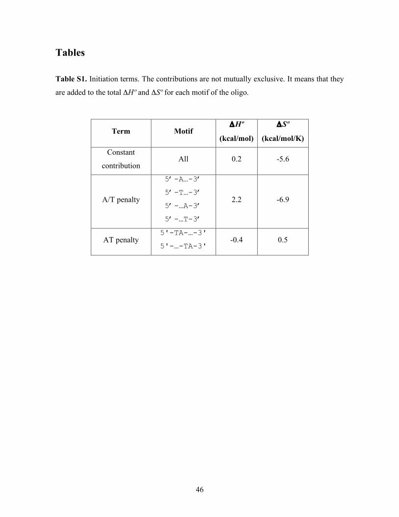
temperature nor the salt concentration (see Table S1). To extend the prediction of the

melting temperatures to different salt conditions, the salt dependence of the entropy has to

be considered. The Unified Oligonucleotide (UO) model predicts the melting temperature

at different salt conditions assuming a homogeneous correction for all the 10 NNBP. At a

salt condition [Mon+] (where [Mon+] is the total concentration of monovalent ions)

different from 1 M NaCl, the UO model corrects ΔSº according to

17

!

"S0([Mon

+]) = "S

0(1 M NaCl) + 0.368 # N # ln[Mon

+] [10]

where N is the number of phosphates divided by 2 (i.e. the number of base pairs of the

hairpin). Our heterogeneous salt correction assumes a different prefactor for each NNBP,

which is temperature independent. Therefore, the entropy of an oligo is corrected according

to

!

"S0([Na

+]) = "S0

(1 M NaCl) +m

i(T)

Ti=1

N

# ln[Mon+] [11]

where mi(T) are the specific salt corrections at T = 298 K and they have to be summed over

all N base pairs of the hairpin. Note that the prefactor mi(T)/T is independent of the

temperature. Following this scheme we find that our heterogeneous salt correction gives the

following prediction for the melting temperatures,

!

TM

="H 0

"S0 +m

i(T)

Ti=1

N

# ln[Mon+]+ R ln C

T/4[ ]

[12]

which is Equation 4 of the main text.

S9. Enthalpy and entropy inference

Our unzipping experiments provide direct measurements of the free energies (εi) and the

salt correction (mi) at T = 298 K for all the NNBP (i = 1,...,10), but no information about

the enthalpy (Δhi) and the entropy (Δsi) is provided. However, combining our results with

the measurements of melting temperatures of several oligos obtained by optical melting

experiments we can infer the enthalpies and the entropies. In order to do so, we define an

error function (χ2) that accounts for the mean squared error between the experimental

18

melting temperatures (7) (

!

Tiexp ) and the predicted (

!

Tipred ) ones for N different oligos and salt

conditions,

( )! ""#=""N

i

pred

i

exp

iNhhTThh

2

1011

101

2 ),,(),,( KK$ [13]

where Δhi (i=1,...,10) are the NNBP enthalpies and

!

Tipred are obtained according to Eq. 12

The NNBP entropies are fixed by 10 constraints that relate the free energies, the enthalpies

and the entropies according to

!

"i= #h

i$T#s

i % #s

i=#h

i$"

i

T [14]

where i = 1,...,10; εi are the experimentally measured free energies with unzipping and

T = 298 K. Here, the enthalpies are fitting parameters that fix the entropies. Therefore the

enthalpies and the entropies are fully correlated (their correlation coefficients are equal

to 1). The error function is minimized with respect to the enthalpies using a steepest descent

algorithm that rapidly converges to the same solution when starting from different initial

conditions.

Here we provide and estimation of the error (

!

"#hi

) of the 10 fitting parameters Δhi0

(i = 1,...,10). We simplify the notation by writing the Δhi0 (i=1,...10) values that we give in

Table 2 main text in vectorial form according to

!

"hm

#

, where m stands for minimum. Note

that

!

"hm

#

minimizes the

!

" 2(#h$

) error function (Eq. 13). By definition, the first derivatives

of

!

" 2(#h$

) with respect to

!

"h#

vanish at the minimum (

!

r " # $ 2(%h

m

&

) = 0). So we can write a

Taylor expansion of

!

" 2(#h$

) up to second order according to:

!

" 2(#hm

$

+ %#h$

) & " 2(#hm

$

) +1

2%#hT '

$

H " 2(#hm

$

)(

) *

+

, - ' %#h

$

[15]

19

where

!

"#h$

is a variation of the

!

"hm

#

vector and

!

H(" 2(#hm

$

)) is the Hessian matrix of

second derivaties

!

Hij =" 2# 2

($h1

0,...,$h

10

0)

"$hi0 "$h j

0 evaluated at the minimum

!

"hm

#

. Our estimation

of

!

" 2(#hm

$

) =1.74 (in units of squared Celsius degrees ºC2) is lower than the typical

experimental error in melting experiments, which is 2 ºC (i.e

!

" 2 = 4 ). So there is a range of

!

"h#

values around the minimum

!

"hm

#

that still predict the melting energies within an

average error of 2 ºC. This range of values is what determines the error in the estimation of

!

"hm

#

. Following this criterion, we look for the variations around the minimum (

!

"#h$

) that

produce a quadratic error of 4 ºC2. We divide this quadratic error into the 10 fitting

parameters (Δhi0 i=1,…,10) and the 10 related ones (Δsi

0 i=1,…,10). So we look for each

!

"#hi that induces an error or 4 ºC2/20 = 0.2 ºC2. Now, introducing

!

" 2(#hm

$

+ %#h$

) = 4 and

!

" 2(#hm

$

) =1.74 into Eq. 15 and isolating

!

"#h$

, we get one expression to estimate the errors

of the 10 fitting parameters:

!

"#hi=$#h

i

=2 % (0.2 & 0.087)

Hii(' 2

(#hm

(

))

=0.226

Hii(' 2

(#hm

(

))

, i =1,...,10 [16]

which gives values between 0.3 - 0.6 kcal/mol (see Table 2 main text). Now, the error in

the estimation of the entropies (

!

"#si

) can be obtained from error propagation of Eq. 14:

!

"#si

=1

T"#s

i

+"#$i

( ), i =1,...,10 [17]

where T = 298.15 K is the temperature and

!

"#$i

are the experimental errors of our estimated

NNBP energies from the unzipping measurements (Table 1, main text). The errors range

between 1.2 - 2.2 cal/mol·K (Table 2, main text). Our results are compatible with the UO

enthalpies and entropies.

20

S10. Free energy of the loop

The end loop of the molecule is a group of 4 bases that forms a structure that facilitates the

rezipping of the two strands of the dsDNA hairpin. The free energy formation of the loop

gets contributions from the bending energy, the stacking of the bases in the loop and the

loss of entropy of the ssDNA. The energy formation of the loop is positive, meaning that

the loop is an unstable structure at zero force. Upon decreasing the total extension, the

formation of complementary base pairs along the sequence reduces the total energy of the

molecule and the loop can be formed.

The effect of the loop is appreciated only in the last rip of the FDC. It introduces a

correction to the free energy of the fully extended ssDNA molecule and modifies the force

at which the last rip is observed (Figure S13).

S11. Sampling of energy states distribution

According to the NN model, the energy of the DNA duplex is higher when more base pairs

are open. In our experiments, the opening of base pairs is sequential, meaning that the base

pair that is closest to the opening fork is the one that dissociates first. As the molecule is

pulled, the unzipping fork that separates the ssDNA from the dsDNA progressively

advances as more dsDNA is converted into released ssDNA (see Figure S14a). This can be

achieved thanks to the stiffness of the parabolic trap potential, which is high enough to

allow us to progressively unzip the molecular construct and access to any particular region

of the sequence. The position of the unzipping fork is determined by the number of open

base pairs, which minimizes the total energy of the system at a fixed distance (i.e. at a fixed

trap position). In general, the position of the unzipping fork (even at a fixed distance)

exhibits thermally induced fluctuations in such a way that the system can explore higher

free energy states. Such fluctuations represent the first kind of excitations in the system and

will be discussed in the next paragraphs. However there is a second kind of excitation:

breathing fluctuations. The breathing is the spontaneous opening and closing of base pairs

21

produced in the dsDNA, far away from the unzipping fork (see Figure S14b). During this

process, the DNA explores states of higher free energy while the unzipping fork is kept at

the same position. So the breathing does not induce any change in the position of the

unzipping fork. Consequently, we are not able to distinguish the breathing in our unzipping

experiments because breathing fluctuations are not coupled to the reaction coordinate that

we measure, i.e. the molecular extension, and should have a small effect on the measured

FDC. Note that breathing fluctuations are expected to be relevant only at high enough

temperatures. While the inclusion of breathing fluctuations should be considered at high

enough temperatures their contribution at 25ºC is expected to be minimal. The fact that our

model reproduces very well the experimental FDC supports this conclusion.

Now let us focus on the fluctuations of the unzipping fork. As explained in the manuscript,

the unzipping of DNA is performed at very low pulling rate in our experiments. The pulling

process is so slow that the system reaches the equilibrium at every fixed distance along the

pulling protocol. Figure S15a shows a fragment of the FDC in a region where 3 states

having different number of open base pairs coexist (n1=1193, n2=1248 and n3=1300).

Figure S15b shows the hopping in force due to the transitions that occur between these 3

states. The slow pulling rate guarantees that the hopping transitions are measured during

unzipping (i.e. many hopping events take place while the molecule is slowly unzipped).

The filtering of the raw FDC data produces a reasonably good estimation of the equilibrium

FDC. It is also important to remark that the unzipping and rezipping curves are reversible

(see Fig. 1c main text). This supports the idea that the unzipping process is quasistatic and

correctly samples the energy states.

In general, the hopping frequency between coexistent states is around ~10 - 50 Hz and the

area of coexistence extends over 40 nm of distance. At a pulling rate of 10 nm/s, we can

measure around 10-40 transitions, which in most cases is sufficient to obtain a good

estimation of the FDC after averaging out the raw data.

Figure S16a shows the free energy landscape of one molecule at different fixed distances,

which is given by G(xtot,n) in Eq. 1 main text (see also the subsection Calculation of the

22

equilibrium FDC in the Materials and Methods section in main). A detailed view of the

free energy landscape (see Figure S16b) shows that it is a rough function and its coarse

grained shape is parabolic. It means that for each value of xtot there is always a state of

minimum global energy surrounded by other states of higher free energies (see

Figure S16b). Although there are lots of states in phase space, in the experiments we only

observe those states that differ in free energy by less than ~5 kBT with respect to the state of

minimum free energy. So the hopping transitions described in Figure S15 are between

states that have similar free energies. Outside this range of free energies, the higher

energetic states are rarely observed and their contribution to the equilibrium FDC is

negligible.

Summing up, the sufficiently high trap stiffness, the short length of the molecular handles,

the slow pulling rate and the shape of the free energy landscape ensure us that we explore

higher energetic states (within a range of ~5 kBT with respect to the global minimum)

during the unzipping process. Therefore, the averaged FDC is a good estimation of the

equilibrium FDC.

S12. Thermodynamics of DNA unzipping

The state of the system is determined by the number of open bp and the position of the

center of the trap that fixes the total distance of the system. These two parameters and the

force allow us to understand the process the molecule undergoes in an unzipping

experiment. A useful three-dimensional representation of the space of variables is shown in

Figure S17. The experiment starts when the molecule is closed and relaxed. We call this

state A, in which the distance, the force and the number of open bps are equal to 0. The

molecule unzips as the total distance increases (red curve). When the molecule is fully

extended and stretched, the system is in the state B. The state C corresponds to a relaxed

random coil of ssDNA. The free energy of formation of the duplex is equal to the sum of all

NNBP energy contributions along the sequence and is given by the difference in free

energy between states A and C. C is an inaccessible experimental state because ssDNA

23

forms secondary structures at low forces. However, C can be recovered theoretically from

B by considering that the fully extended molecule behaves like a random coil without

interactions and is accurately described by an elastic polymer model.

S13. Dependence of the optimization algorithm on the initial

conditions

We have carried out a detailed study of the optimization algorithm in order to check that the

final solution does not depend on the initial conditions given to the algorithm. An ensemble

of initial conditions where selected from the values of the different labs that were unified

by SantaLucia (6) (Figure S18a). The FDCs predicted by the different energy values are

depicted in Figure S18c. Here we can observe how an overestimation (underestimation) in

absolute value of the NNBP energies leads to an overestimation (underestimation) of the

mean unzipping force. The same elastic properties (ssDNA, handles and optical trap) have

been used in all cases. Figure S18b shows the optimal values of the NNBP energies for the

ensemble of initial conditions. All the NNBP energies have an error smaller than

0.1 kcal/mol. Our optimization algorithm converges to essentially the same solution when

starting from various initial conditions because the error bars of the different solutions

obtained for each initial condition overlap with each other. Figure S18d shows the final

FDCs obtained when using the optimal values of the NNBP energies obtained for each

initial condition. The different FDCs are indistinguishable and they reproduce

quantitatively the experimental FDC.

S14. Errors in the Monte Carlo optimization

There are three kinds of errors at different levels that we will denote as σ1, σ2, σ3 :

24

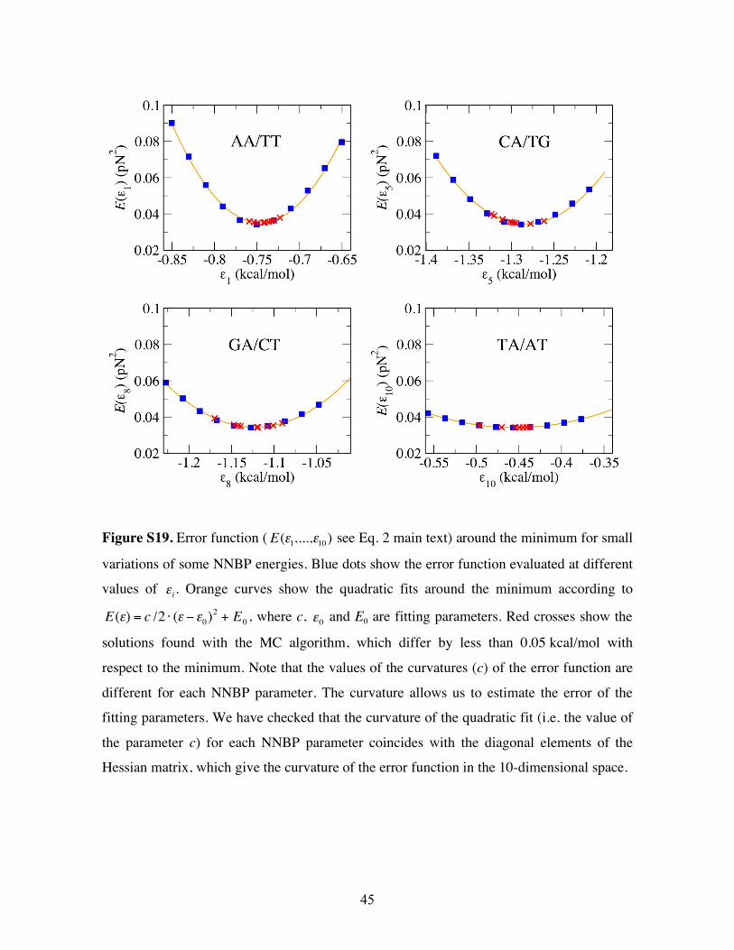
1. The first error σ1 comes from the fitting algorithm. The uncertainties of the

estimated NNBP energies (

!

"#i

) indicate how much the error function

(

!

E("1,...,"

10,"loop ) see Eq. 2 main text) changes when the fitting parameters

!

"i are

varied around the minimum. For instance, a variation of the AA/TT motif (

!

"#1)

around the minimum (see Figure S19) produces a larger change in the error function

than a variation of the TA/AT motif (

!

"#10

). This indicates that the uncertainty of

AA/TT is lower than that of TA/AT. The curvature of the minimum in each

direction

!

"i gives the uncertainty. There is a different set of

!

"#i

uncertainties for

each fit (i.e. each molecule). A quantitative evaluation of the uncertainty of the

NNBP parameters requires the evaluation of the χ2 function for each FDC (i.e. each

fit), which is given by:

!

" 2(r # ) =

fi $ f (xi;r # )

% y

&

' ( (

)

* + +

i=1

N

,2

[18]

where N is the number of experimental points of the FDC; xi and fi are the position

and the force measurements, respectively;

!

r " is the vector of fitting parameters

{

!

"i} i = 1,...10;

!

f (xi;r " ) is the theoretically predicted FDC according to the model

(see Calculation of the equilibrium FDC in the Materials and Methods section in

main text); and σy is the experimental error of the force measurements performed

with the optical tweezers. As indicated in section S2, the resolution of the

instrument is σy = 0.1 pN. The uncertainty of the fit parameters is given by the

following expression (8):

!

"#i

= Cii

[19]

where Cii are the diagonal elements of the variance-covariance matrix Cij. In a non-

linear least square fit, this matrix can be obtained from

!

Cij = 2 "Hij

#1, where

!

Hij

"1 is

the inverse of the Hessian matrix

!

Hij =" 2# 2(

r $ m )

"$i"$ j of

!

" 2(r # ) evaluated at point

!

r " m

that

minimizes the error. Note that the error function and the χ2 function are related by a

constant factor,

!

" 2(r # ) = N /$ y

2( ) % E(r # ), so their Hessians are related by one constant

factor, as well. The calculation of

!

"#i

is quite straightforward and it gives values

25

between 0.003-0.015 kcal/mol. These values represent the first type of error that we

call σ1. Note that the Hessian matrix evaluated at the minima found with the heat-

quench algorithm is very similar to the Hessian matrix evaluated at the minimum,

which means that the curvature is almost the same in all heat-quench minima.

Therefore the error of the fit σ1 takes the same value within a region of

±0.1 kcal/mol.

2. The second error comes from the dispersion of the heat-quench minima. As we saw

previously, there are several minima corresponding to different possible solutions

(each solution being a set of 10 NNBP energies) for the same molecule. The values

of the NNBP energies corresponding to the different solutions are Gaussian

distributed (see Figure S10c) and the average standard deviation is about

0.05 kcal/mol. All these considerations result in a second typical error

σ2 = 0.05 kcal/mol.

3. Finally, the third error corresponds to the molecular heterogeneity intrinsic to single

molecule experiments. Such heterogeneity results in a variability of solutions

among different molecules. Indeed, the FDCs of the molecules are never identical

and this variability leads to differences in the values of the NNBP energies. This

variability is the major source of error in the estimation of our results. The error bars

in Figs. 2d,e and 3 (main text) indicate the standard error of the mean, which is

around 0.1 kcal/mol on average. This is what finally determines the statistical error

of our analysis, σ3 = 0.1 kcal/mol.

Since the major source of errors is the variability of the results from molecule to molecule,

we simply report this last error in the manuscript. Because σ3 > σ2 > σ1 we can safely

conclude that the propagation of the errors of the heat-quench algorithm will not increase

the final value of the error bar.

26

REFERENCES

1. Smith SB, Cui Y, Bustamante C (2003) Optical-trap force transducer that operates by

direct measurement of light momentum. Methods Enzymol. 361:134-160.

2. Bustamante C, Smith SB (2006) Light-Force sensor and method for measuring axial

optical-trap forces from changes in light momentum along an optical axis. U.S. Patent

7,133,132 B2.

3. Bustamante C, Smith SB (2006) Optical beam translation device and method using a

pivoting optical fiber. U.S. Patent 7,274,451 B2.

4. http://tweezerslab.unipr.it

5. Kirkpatrick S, Gelatt CD Jr, Vecchi MP. (1983) Optimization by simulated annealing.

Science 220:671-680

6. Santalucia J Jr. (1998) A unified view of polymer, dumbbell, and oligonucleotide DNA

nearest-neighbor thermodynamics. Proc Nat Acad Sci USA 95:1460-1465.

7. Owczarzy R, You Y, Moreira BG, Manthey JA, Huang L, Behlke MA, Walder JA

(2004) Effects of sodium ions on DNA duplex oligomers: improved predictions of

melting temperatures. Biochemistry 43:3537-3554.

8. Press WH, Teukolsky SA, Vetterling WT, Flannery BP. (1992) Numerical Recipes in

C: The Art of Scientific Computing. (2nd Ed. Cambridge University Press, New York).

27

Figures

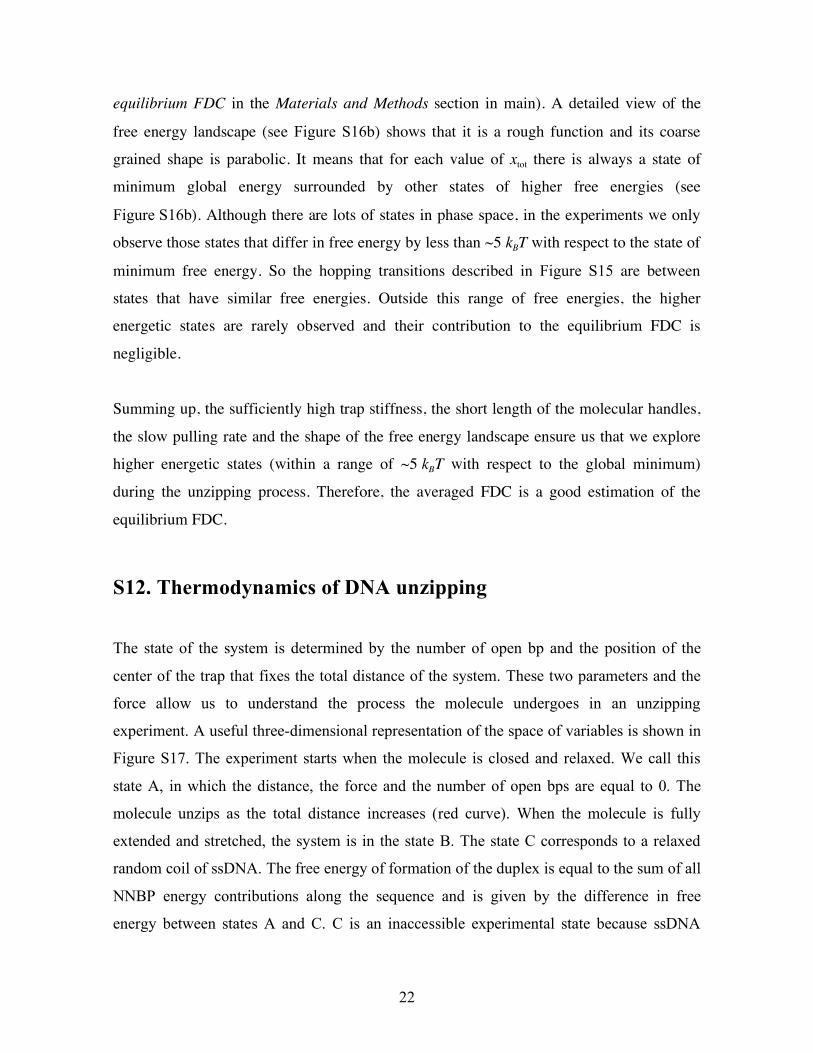
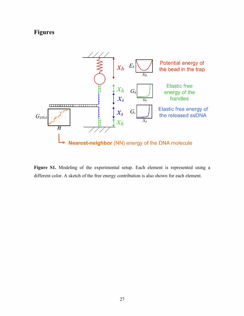
Figure S1. Modeling of the experimental setup. Each element is represented using a

different color. A sketch of the free energy contribution is also shown for each element.

28

Figure S2. Experimental setup. The configuration is symmetric for each laser. Two fiber-coupled diodes

lasers, Lumix LU845-200mW (LA & LB) feed power to twin fiber wigglers (WA & WB). The optical

fiber is bent at the wiggler using piezo crystals and the laser beams can be redirected at will so that they

can be repositioned. Part of the light is used to form “light-lever” position detectors by using pellicle

beamsplitters (PSA & PSB), refocusing lenses (RFA & RFB) and position-sensitive detectors (LLA &

LLB). The remaining light is collimated as beams by using two lenses (CA & CB) and then the beams are

introduced into the optical axis by using polarizing beamsplitters (PBS2, PBS3). Two λ/4 plates produce

circular polarization before the beams are focused by two Olympus 60x water-immersion microscope

objectives with NA=1.2 (OA & OB). The exiting light is collected by the opposite objective (OB & OA),

returned to linear (orthogonal) polarization by the λ/4 plates (λB & λA) and redirected to the (OSI

Optoelectronics, DL-10) position-sensitive detectors (PSDA & PSDB) by combining the effect of the

PBS and the relay lenses (RA & RB). The PSDs detect transverse (X, Y) forces while a so-called “Iris

Sensor” detects changes in the axial light-momentum flux to infer the Z-axis force (2). A blue LED and a

CCD camera are used to form a microscope to view the pipette and beads. The fluidics chamber is

constructed from coverslips and Nescofilm gaskets (4) and its position is controlled by a motorized XYZ

stage.

29

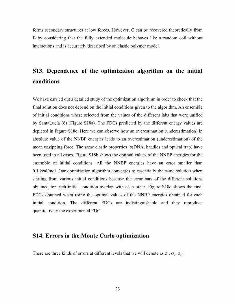
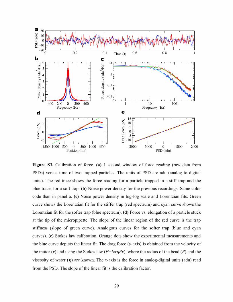
Figure S3. Calibration of force. (a) 1 second window of force reading (raw data from

PSDs) versus time of two trapped particles. The units of PSD are adu (analog to digital

units). The red trace shows the force reading for a particle trapped in a stiff trap and the

blue trace, for a soft trap. (b) Noise power density for the previous recordings. Same color

code than in panel a. (c) Noise power density in log-log scale and Lorentzian fits. Green

curve shows the Lorentzian fit for the stiffer trap (red spectrum) and cyan curve shows the

Lorentzian fit for the softer trap (blue spectrum). (d) Force vs. elongation of a particle stuck

at the tip of the micropipette. The slope of the linear region of the red curve is the trap

stiffness (slope of green curve). Analogous curves for the softer trap (blue and cyan

curves). (e) Stokes law calibration. Orange dots show the experimental measurements and

the blue curve depicts the linear fit. The drag force (y-axis) is obtained from the velocity of

the motor (v) and using the Stokes law (F=6πηRv), where the radius of the bead (R) and the

viscosity of water (η) are known. The x-axis is the force in analog-digital units (adu) read

from the PSD. The slope of the linear fit is the calibration factor.

30

Figure S4. Measurements in two optical tweezers instruments. Black curve shows the

unzipping data of a 2.2 kb molecule in the Berkeley setup. The data is shown as Force vs.

Extension Curve (FEC). Red, blue and green curves show the data of 3 different molecules

obtained with the Barcelona instrument. The FEC has been obtained from the FDC by

subtracting the force/distance compliance of the optical trap.

31

Figure S5. Calibration of distance. (a) Protocol to calibrate the light-lever position. A bead

is held fixed at the tip of the micropipette. The optical trap is set to keep zero force with a

force feedback algorithm operating at 4 kHz. As the pipette is gently moved the trap

follows the center of the bead to maintain the preset zero force. The micropipette is moved

up and down (blue arrow) to calibrate the y distance and left and right (orange arrow) to

calibrate the x distance. The gray square (side length of 11 µm) shows the range of the

piezos. The position of the micropipette is obtained from the shaft encoders of the motors

and the position of the trap is obtained from the light-levers. (b) Calibration of y distance

for trap A. The black curve is obtained moving the trap up and down. Green line shows the

linear fit when the bead is moved downwards. The slope of the line is the calibration factor

for the y distance of trap A. Red line shows the linear fit when the bead is moved upwards.

Both branches (green and red) do not overlap because the motor has a backslash. During

the backslash, the shaft encoder of the motor detects rotation but the gears actually do not

rotate. (c) Calibration of y distance for trap B. The same procedure as in (b).

32

Figure S6. Molecular construction. A sequence of 6770 bp obtained from λ-DNA is ligated

to a tetraloop and two short handles.

33

Figure S7. Synthesis of the 3 kb molecular construct. The denaturated ssDNA molecule

can be stretched between two coated beads, since the Biotin and Digoxigenins labels are

located on the same strand.

34

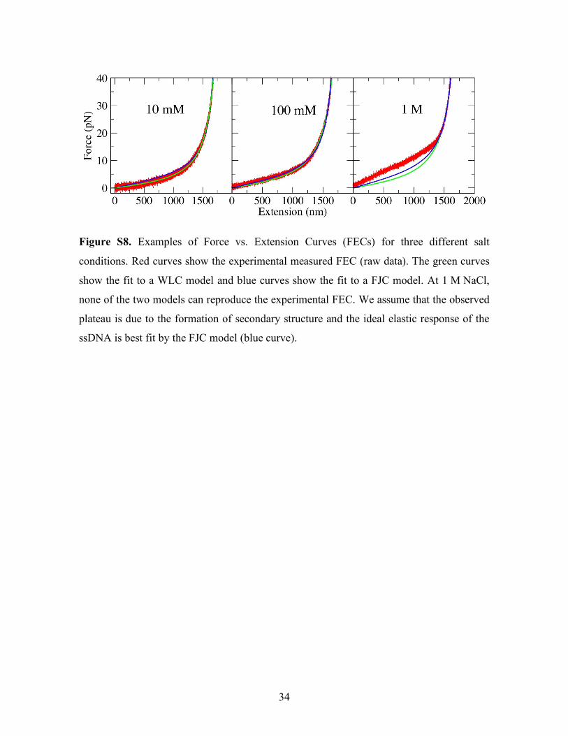
Figure S8. Examples of Force vs. Extension Curves (FECs) for three different salt

conditions. Red curves show the experimental measured FEC (raw data). The green curves

show the fit to a WLC model and blue curves show the fit to a FJC model. At 1 M NaCl,

none of the two models can reproduce the experimental FEC. We assume that the observed

plateau is due to the formation of secondary structure and the ideal elastic response of the

ssDNA is best fit by the FJC model (blue curve).

35

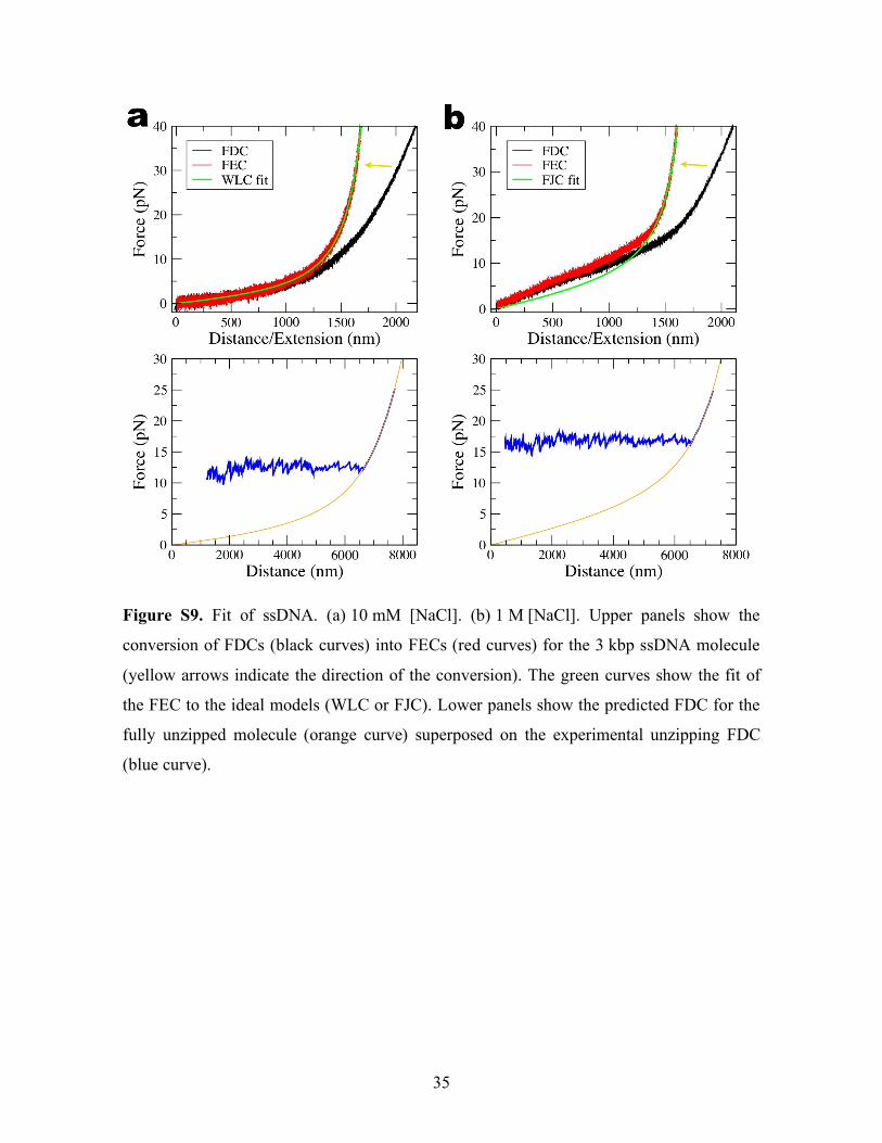
Figure S9. Fit of ssDNA. (a) 10 mM [NaCl]. (b) 1 M [NaCl]. Upper panels show the

conversion of FDCs (black curves) into FECs (red curves) for the 3 kbp ssDNA molecule

(yellow arrows indicate the direction of the conversion). The green curves show the fit of

the FEC to the ideal models (WLC or FJC). Lower panels show the predicted FDC for the

fully unzipped molecule (orange curve) superposed on the experimental unzipping FDC

(blue curve).

36

Figure S10. (a) Evolution of the error function of different molecules during the quenching

minimization. The main figure shows a log-log plot where the mean quadratic error

decreases down close to 0.01 pN2. The inset figure shows a linear plot of the same

evolution. (b) Evolution of the error during the heat-quench algorithm. (c) Histograms of

solutions for one representative molecule obtained using the heat-quench algorithm. Each

color represents one NNBP parameter and its Gaussian fit profile. Optimal solutions

correspond to the most probable values of the distribution.

37

Figure S11. Fit of the shift function. (a) Step 1. (b) Steps 1,2 and 3. (c) Step 4. (d) Steps

4,5 and 7. (e) Step 6. (f) Step 7. (g) Step 7.

38

Figure S12. Shift function. The figure shows the shift function for some 6.8 kb molecules

at different salt conditions. The inset shows the shift function for different molecules of

2.2 kbp at 500 mM NaCl (=red) and 1 M NaCl (=green). The grey shaded region

corresponds to trap positions where DNA is fully unzipped. In this region, the local shift

nearly vanishes.

39

Figure S13. Effect of the loop contribution. The free energy of the loop modifies the shape

of the theoretical FDC only at the last rip just before the elastic response of the full ssDNA

is observed. The black curve is the experimental FDC. All other curves show theoretical

FDCs with different values of εloop. Red curve, best fit with εloop=2.27 kcal/mol; magenta

curve, εloop=0.0 kcal/mol; green curve, εloop=1.00 kcal/mol; blue curve, εloop=2.00 kcal/mol

and orange curve, εloop=3.00 kcal/mol.

40

Figure S14. (a) Opening fork. (b) Breathing.

41

Figure S15. Coexistence of states. (a) Left panel shows the measured FDC for the 2.2 kbp

sequence. Right panel shows the fragment of the FDC (framed in the left panel) where 3

states coexist. Red curve shows the raw data and black curve shows the data filtered at

1 Hz. (b) Red curve shows the force vs. time of the previous fragment where the transitions

between these 3 states can be observed. The blue lines indicate the average forces

corresponding to each of these 3 states.

42

Figure S16. Free energy landscape for the 2.2 kb sequence at fixed distance. (a) The

parabolic-like shape of the free energy landscape around the minima can be identified in a

coarse grained view of what in truth is a rough landscape (see zoomed part of the

landscape). Black, orange, green, blue, yellow, magenta and red curves show the free

energy landscape at xtot = 0,350, 500, 750, 1000, 1250 and 1455 nm, respectively. (b)

Zoomed region of the free energy landscape at the distance in which the 3 states of

Figure S15 coexist. The blue arrows indicate the minima that correspond to these states.

The highlighted gray area shows an energy range of 5 kBT .

43

Figure S17. Equation of state of the 6.8 kb molecular construct. The red curve shows an

equilibrium unzipping process in which the number of open bps increases as the total

distance is increased. The projection of this process on the force-distance plane gives the

FDC and is experimentally measured (green curve). The projection on the distance-open bp

plane is shown in blue. The elastic response of the fully opened molecule is depicted in

magenta (the projection in the Force-Distance plane is also depicted in magenta). A is the

initial state in an unzipping experiment and B is the final state. A is the native state of the

molecular construct. State B corresponds to a stretched random coil. C is an experimentally

inaccessible state, which corresponds to a relaxed random coil.

44

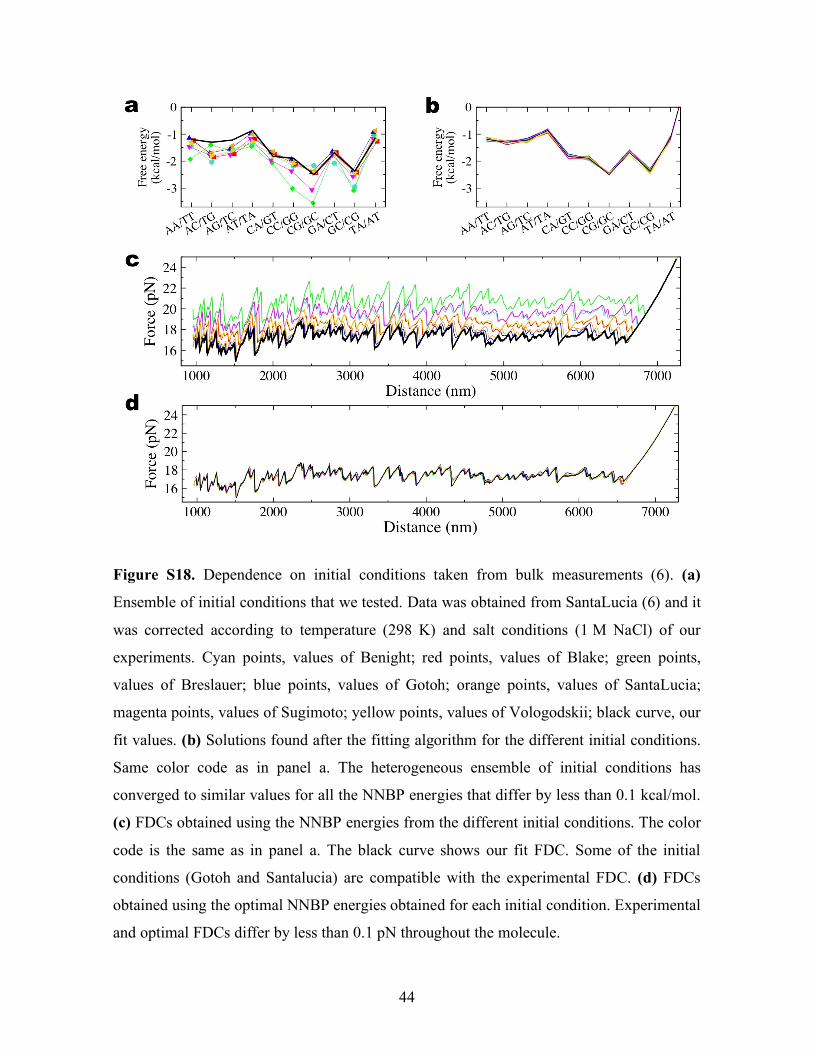
Figure S18. Dependence on initial conditions taken from bulk measurements (6). (a)

Ensemble of initial conditions that we tested. Data was obtained from SantaLucia (6) and it

was corrected according to temperature (298 K) and salt conditions (1 M NaCl) of our

experiments. Cyan points, values of Benight; red points, values of Blake; green points,

values of Breslauer; blue points, values of Gotoh; orange points, values of SantaLucia;

magenta points, values of Sugimoto; yellow points, values of Vologodskii; black curve, our

fit values. (b) Solutions found after the fitting algorithm for the different initial conditions.

Same color code as in panel a. The heterogeneous ensemble of initial conditions has

converged to similar values for all the NNBP energies that differ by less than 0.1 kcal/mol.

(c) FDCs obtained using the NNBP energies from the different initial conditions. The color

code is the same as in panel a. The black curve shows our fit FDC. Some of the initial

conditions (Gotoh and Santalucia) are compatible with the experimental FDC. (d) FDCs

obtained using the optimal NNBP energies obtained for each initial condition. Experimental

and optimal FDCs differ by less than 0.1 pN throughout the molecule.

45

Figure S19. Error function (

!

E("1,...,"

10) see Eq. 2 main text) around the minimum for small

variations of some NNBP energies. Blue dots show the error function evaluated at different

values of

!

"i. Orange curves show the quadratic fits around the minimum according to

!

E(") = c /2 # (" $"0)2

+ E0, where c,

!

"0 and E0 are fitting parameters. Red crosses show the

solutions found with the MC algorithm, which differ by less than 0.05 kcal/mol with

respect to the minimum. Note that the values of the curvatures (c) of the error function are

different for each NNBP parameter. The curvature allows us to estimate the error of the

fitting parameters. We have checked that the curvature of the quadratic fit (i.e. the value of

the parameter c) for each NNBP parameter coincides with the diagonal elements of the

Hessian matrix, which give the curvature of the error function in the 10-dimensional space.

46

Tables Table S1. Initiation terms. The contributions are not mutually exclusive. It means that they

are added to the total ΔHº and ΔSº for each motif of the oligo.

Term Motif ΔHº

(kcal/mol)

ΔSº

(kcal/mol/K)

Constant

contribution All 0.2 -5.6

A/T penalty

5’-A…-3’

5’-T…-3’

5’-…A-3’

5’-…T-3’

2.2 -6.9

AT penalty 5'-TA-…-3'

5'-…-TA-3' -0.4 0.5

47

Sal

t

Seq

uenc

e 5'

-…-3

' Te

TUO

Tu

Te

TUO

Tu

Te

TUO

Tu

Te

TUO

Tu

Te

TUO

Tu

ATCAATCATA

21.3

21.7

19.3

24.5

24.1

22.1

27.9

26.9

25.2

32.4

31.7

30.7

33.6

34.0

33.4

TTGTAGTCAT

24.7

24.5

20.7

28.2

26.9

23.2

31.2

29.6

26.1

34.8

34.4

31.0

36.0

36.7

33.5

GAAATGAAAG

22.1

23.2

18.6

25.3

25.5

21.3

29.1

28.0

24.4

33.1

32.5

29.9

34.4

34.6

32.6

CCAACTTCTT

29.0

28.3

24.2

32.1

30.7

26.7

35.9

33.4

29.5

39.6

38.1

34.5

40.6

40.4

36.9

ATCGTCTGGA

33.8

33.8

29.6

37.4

36.2

32.3

40.5

39.0

35.4

44.5

43.8

40.7

44.9

46.2

43.3

AGCGTAAGTC

27.4

33.3

29.5

31.2

35.6

31.9

34.6

38.3

34.7

39.5

42.9

39.4

40.3

45.1

41.8

CGATCTGCGA

39.2

38.8

35.0

42.3

41.1

37.6

45.6

43.7

40.6

48.4

48.3

45.7

49.1

50.5

48.2

TGGCGAGCAC

44.4

44.2

41.5

47.8

46.6

43.5

51.3

49.3

45.8

55.0

54.0

49.9

55.3

56.3

51.8

GATGCGCTCG

44.2

42.6

39.7

47.0

44.8

42.1

50.1

47.4

44.8

53.6

51.8

49.4

53.5

54.0

51.7

GGGACCGCCT

46.7

45.9

43.4

50.3

48.4

45.3

53.1

51.3

47.6

56.5

56.2

51.4

57.0

58.6

53.3

CGTACACATGC

40.4

39.5

37.8

43.5

41.8

40.0

46.1

44.4

42.5

49.6

49.0

46.8

49.9

51.2

48.9

CCATTGCTACC

38.0

37.4

36.4

41.7

39.8

38.4

44.5

42.5

40.7

47.9

47.3

44.7

48.9

49.6

46.6

TACTAACATTAACTA

35.3

38.6

37.3

40.4

41.2

39.9

44.1

44.2

43.0

49.3

49.4

48.2

51.1

51.9

50.8

ATACTTACTGATTAG

38.1

36.7

35.7

41.4

39.2

38.4

45.0

42.2

41.5

49.9

47.2

46.8

51.5

49.7

49.4

GTACACTGTCTTATA

41.0

41.7

40.5

44.8

44.3

43.1

48.3

47.2

46.0

52.9

52.3

51.2

54.8

54.8

53.7

GTATGAGAGACTTTA

39.9

41.7

39.4

44.2

44.2

42.2

47.9

47.2

45.5

53.3

52.3

51.1

55.4

54.8

53.9

TTCTACCTATGTGAT

40.6

41.6

40.4

44.6

44.2

43.1

48.1

47.3

46.2

52.3

52.5

51.6

53.7

55.1

54.3

AGTAGTAATCACACC

44.3

43.7

42.7

47.8

46.3

45.2

51.6

49.3

48.2

56.2

54.4

53.3

57.1

56.9

55.8

ATCGTCTCGGTATAA

45.5

45.6

43.4

49.4

48.2

46.4

52.9

51.2

49.7

57.4

56.3

55.6

58.6

58.9

58.5

ACGACAGGTTTACCA

47.8

50.1

48.0

51.2

52.7

50.6

55.5

55.7

53.7

59.8

61.0

58.9

61.3

63.6

61.5

CTTTCATGTCCGCAT

49.9

49.8

48.5

53.9

52.4

51.2

57.1

55.4

54.3

61.4

60.5

59.7

62.8

63.0

62.4

TGGATGTGTGAACAC

46.5

49.1

47.0

51.6

51.7

49.7

54.6

54.7

52.7

59.1

59.8

57.9

60.4

62.3

60.4

ACCCCGCAATACATG

51.3

52.2

51.8

55.2

54.8

54.1

58.5

57.8

56.8

62.4

63.1

61.4

62.9

65.6

63.7

GCAGTGGATGTGAGA

51.2

51.2

49.7

54.8

53.9

52.2

58.0

56.9

55.1

61.7

62.1

60.1

63.3

64.6

62.6

GGTCCTTACTTGGTG

47.8

48.8

47.2

51.6

51.4

49.6

55.1

54.4

52.3

59.1

59.5

57.1

60.3

62.0

59.4

CGCCTCATGCTCATC

52.8

53.5

52.4

56.7

56.0

54.9

60.1

58.9

57.7

63.6

64.0

62.7

65.8

66.5

65.1

AAATAGCCGGGCCGC

59.0

59.3

57.8

62.2

61.9

60.0

65.3

64.9

62.5

69.0

70.2

66.9

70.4

72.7

69.1

CCAGCCAGTCTCTCC

54.1

54.2

53.0

58.0

56.8

55.3

61.5

59.9

57.9

65.1

65.1

62.5

66.7

67.7

64.7

GACGACAAGACCGCG

57.9

57.0

54.2

61.5

59.5

57.0

64.4

62.3

60.1

67.6

67.3

65.6

68.6

69.7

68.2

CAGCCTCGTCGCAGC

60.8

60.1

58.8

64.1

62.6

61.1

67.4

65.6

63.8

70.1

70.6

68.4

72.0

73.0

70.6

CTCGCGGTCGAAGCG

61.5

60.2

57.6

64.6

62.7

60.3

67.1

65.5

63.4

70.0

70.4

68.7

70.7

72.9

71.3

GCGTCGGTCCGGGCT

64.9

64.3

62.0

67.7

67.0

64.4

70.5

70.0

67.1

73.9

75.2

71.9

74.1

77.8

74.2

Mel

tin

g T

emp

era

ture

s (º

C)

69 m

M11

9 m

M22

0 m

M62

1 m

M10

20 m

M

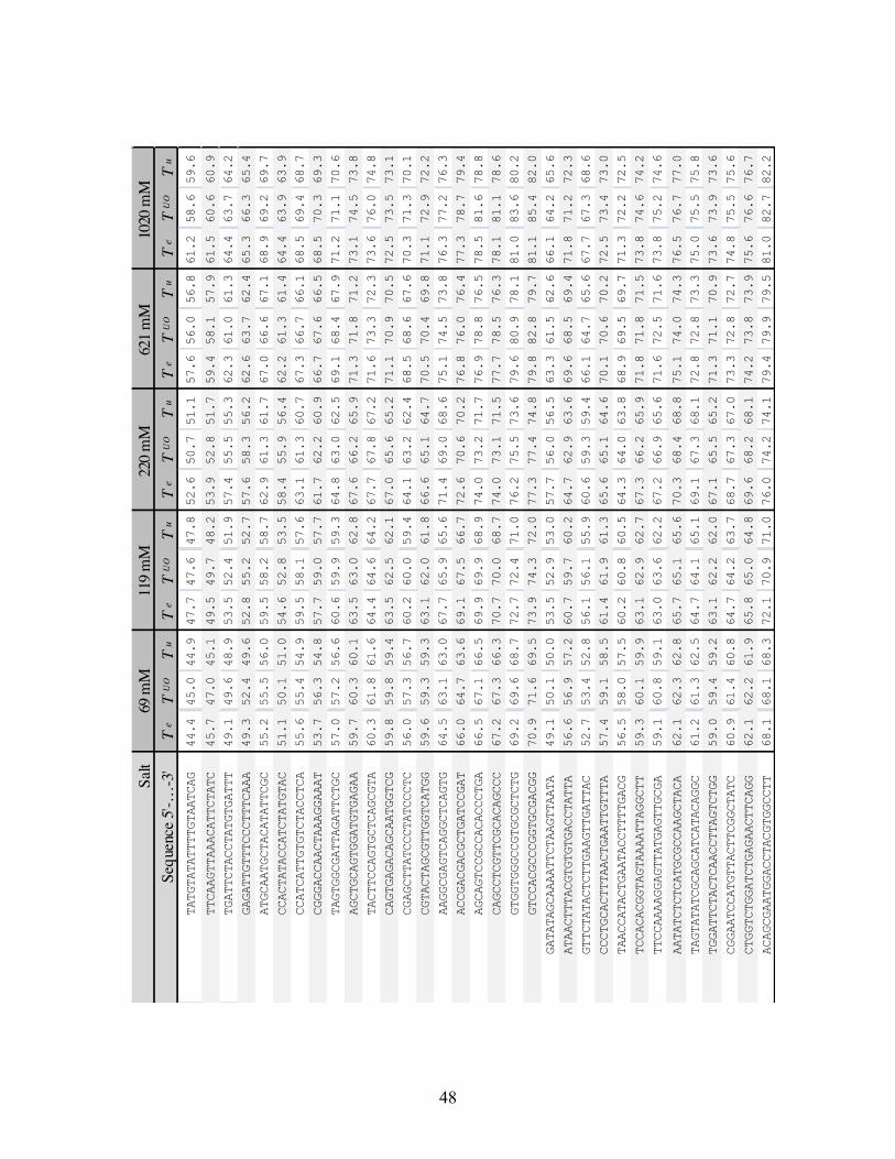
Table S2. Prediction of melting temperatures for the 92 oligos of ref. 7. Te is the

experimental measured temperature in ref. 7. TUO is the Unified Oligonucleotide prediction

obtained with the parameters of ref. 6. Tu is the prediction with our values obtained with

unzipping experiments. Temperatures given in Celsius degrees.

48

Sal

t

Seq

uenc

e 5'

-…-3

' Te

TUO

Tu

Te

TUO

Tu

Te

TUO

Tu

Te

TUO

Tu

Te

TUO

Tu

TATGTATATTTTGTAATCAG

44.4

45.0

44.9

47.7

47.6

47.8

52.6

50.7

51.1

57.6

56.0

56.8

61.2

58.6

59.6

TTCAAGTTAAACATTCTATC

45.7

47.0

45.1

49.5

49.7

48.2

53.9

52.8

51.7

59.4

58.1

57.9

61.5

60.6

60.9

TGATTCTACCTATGTGATTT

49.1

49.6

48.9

53.5

52.4

51.9

57.4

55.5

55.3

62.3

61.0

61.3

64.4

63.7

64.2

GAGATTGTTTCCCTTTCAAA

49.3

52.4

49.6

52.8

55.2

52.7

57.6

58.3

56.2

62.6

63.7

62.4

65.3

66.3

65.4

ATGCAATGCTACATATTCGC

55.2

55.5

56.0

59.5

58.2

58.7

62.9

61.3

61.7

67.0

66.6

67.1

68.9

69.2

69.7

CCACTATACCATCTATGTAC

51.1

50.1

51.0

54.6

52.8

53.5

58.4

55.9

56.4

62.2

61.3

61.4

64.4

63.9

63.9

CCATCATTGTGTCTACCTCA

55.6

55.4

54.9

59.5

58.1

57.6

63.1

61.3

60.7

67.3

66.7

66.1

68.5

69.4

68.7

CGGGACCAACTAAAGGAAAT

53.7

56.3

54.8

57.7

59.0

57.7

61.7

62.2

60.9

66.7

67.6

66.5

68.5

70.3

69.3

TAGTGGCGATTAGATTCTGC

57.0

57.2

56.6

60.6

59.9

59.3

64.8

63.0

62.5

69.1

68.4

67.9

71.2

71.1

70.6

AGCTGCAGTGGATGTGAGAA

59.7

60.3

60.1

63.5

63.0

62.8

67.6

66.2

65.9

71.3

71.8

71.2

73.1

74.5

73.8

TACTTCCAGTGCTCAGCGTA

60.3

61.8

61.6

64.4

64.6

64.2

67.7

67.8

67.2

71.6

73.3

72.3

73.6

76.0

74.8

CAGTGAGACAGCAATGGTCG

59.8

59.8

59.4

63.5

62.5

62.1

67.0

65.6

65.2

71.1

70.9

70.5

72.5

73.5

73.1

CGAGCTTATCCCTATCCCTC

56.0

57.3

56.7

60.2

60.0

59.4

64.1

63.2

62.4

68.5

68.6

67.6

70.3

71.3

70.1

CGTACTAGCGTTGGTCATGG

59.6

59.3

59.3

63.1

62.0

61.8

66.6

65.1

64.7

70.5

70.4

69.8

71.1

72.9

72.2

AAGGCGAGTCAGGCTCAGTG

64.5

63.1

63.0

67.7

65.9

65.6

71.4

69.0

68.6

75.1

74.5

73.8

76.3

77.2

76.3

ACCGACGACGCTGATCCGAT

66.0

64.7

63.6

69.1

67.5

66.7

72.6

70.6

70.2

76.8

76.0

76.4

77.3

78.7

79.4

AGCAGTCCGCCACACCCTGA

66.5

67.1

66.5

69.9

69.9

68.9

74.0

73.2

71.7

76.9

78.8

76.5

78.5

81.6

78.8

CAGCCTCGTTCGCACAGCCC

67.2

67.3

66.3

70.7

70.0

68.7

74.0

73.1

71.5

77.7

78.5

76.3

78.1

81.1

78.6

GTGGTGGGCCGTGCGCTCTG

69.2

69.6

68.7

72.7

72.4

71.0

76.2

75.5

73.6

79.6

80.9

78.1

81.0

83.6

80.2

GTCCACGCCCGGTGCGACGG

70.9

71.6

69.5

73.9

74.3

72.0

77.3

77.4

74.8

79.8

82.8

79.7

81.1

85.4

82.0

GATATAGCAAAATTCTAAGTTAATA

49.1

50.1

50.0

53.5

52.9

53.0

57.7

56.0

56.5

63.3

61.5

62.6

66.1

64.2

65.6

ATAACTTTACGTGTGTGACCTATTA

56.6

56.9

57.2

60.7

59.7

60.2

64.7

62.9

63.6

69.6

68.5

69.4

71.8

71.2

72.3

GTTCTATACTCTTGAAGTTGATTAC

52.7

53.4

52.8

56.1

56.1

55.9

60.6

59.3

59.4

66.1

64.7

65.6

67.7

67.3

68.6

CCCTGCACTTTAACTGAATTGTTTA

57.4

59.1

58.5

61.4

61.9

61.3

65.6

65.1

64.6

70.1

70.6

70.2

72.5

73.4

73.0

TAACCATACTGAATACCTTTTGACG

56.5

58.0

57.5

60.2

60.8

60.5

64.3

64.0

63.8

68.9

69.5

69.7

71.3

72.2

72.5

TCCACACGGTAGTAAAATTAGGCTT

59.3

60.1

59.9

63.1

62.9

62.7

67.3

66.2

65.9

71.8

71.8

71.5

73.8

74.6

74.2

TTCCAAAAGGAGTTATGAGTTGCGA

59.1

60.8

59.1

63.0

63.6

62.2

67.2

66.9

65.6

71.6

72.5

71.6

73.8

75.2

74.6

AATATCTCTCATGCGCCAAGCTACA

62.1

62.3

62.8

65.7

65.1

65.6

70.3

68.4

68.8

75.1

74.0

74.3

76.5

76.7

77.0

TAGTATATCGCAGCATCATACAGGC

61.2

61.3

62.5

64.7

64.1

65.1

69.1

67.3

68.1

72.8

72.8

73.3

75.0

75.5

75.8

TGGATTCTACTCAACCTTAGTCTGG

59.0

59.4

59.2

63.1

62.2

62.0

67.1

65.5

65.2

71.3

71.1

70.9

73.6

73.9

73.6

CGGAATCCATGTTACTTCGGCTATC

60.9

61.4

60.8

64.7

64.2

63.7

68.7

67.3

67.0

73.3

72.8

72.7

74.8

75.5

75.6

CTGGTCTGGATCTGAGAACTTCAGG

62.1

62.2

61.9

65.8

65.0

64.8

69.6

68.2

68.1

74.2

73.8

73.9

75.6

76.6

76.7

ACAGCGAATGGACCTACGTGGCCTT

68.1

68.1

68.3

72.1

70.9

71.0

76.0

74.2

74.1

79.4

79.9

79.5

81.0

82.7

82.2

69 m

M11

9 m

M22

0 m

M62

1 m

M10

20 m

M

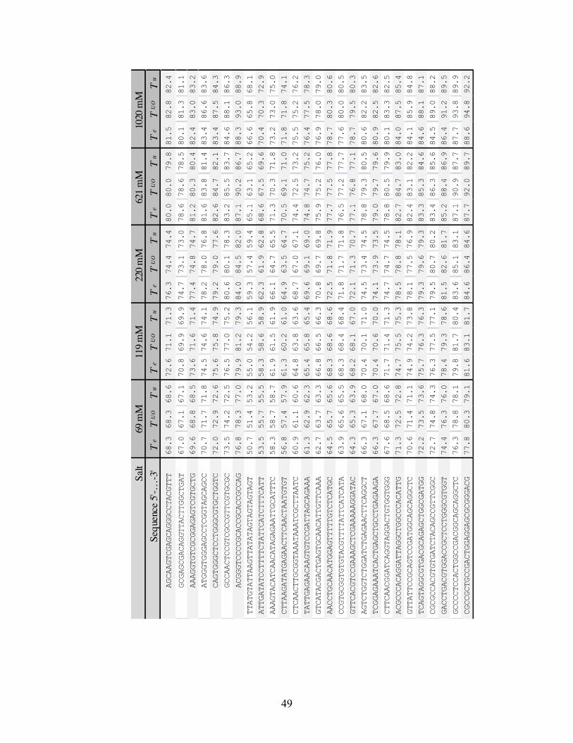
49

Sal

t

Seq

uenc

e 5'

-…-3

' Te

TUO

Tu

Te

TUO

Tu

Te

TUO

Tu

Te

TUO

Tu

Te

TUO

Tu

AGCAAGTCGAGCAGGGCCTACGTTT

68.3

68.3

68.6

72.6

71.1

71.3

76.3

74.4

74.4

80.0

80.0

79.8

81.5

82.8

82.4

GCGAGCGACAGGTTACTTGGCTGAT

67.0

67.1

67.1

70.8

69.9

69.9

74.7

73.1

73.0

78.6

78.6

78.5

80.1

81.3

81.1

AAAGGTGTCGCGGAGAGTCGTGCTG

69.6

68.8

68.5

73.6

71.6

71.4

77.4

74.8

74.7

81.2

80.3

80.4

82.4

83.0

83.2

ATGGGTGGGAGCCTCGGTAGCAGCC

70.7

71.7

71.8

74.5

74.6

74.1

78.2

78.0

76.8

81.6

83.8

81.4

83.4

86.6

83.6

CAGTGGGCTCCTGGGCGTGCTGGTC

72.0

72.9

72.6

75.6

75.8

74.9

79.2

79.0

77.6

82.6

84.7

82.1

83.4

87.5

84.3

GCCAACTCCGTCGCCGTTCGTGCGC

73.5

74.2

72.5

76.5

77.0

75.2

80.6

80.1

78.3

83.2

85.5

83.7

84.6

88.1

86.3

ACGGGTCCCCGCACCGCACCGCCAG

76.8

78.3

77.0

79.9

81.2

79.3

84.0

84.5

82.0

87.1

90.2

86.7

88.3

93.0

88.9

TTATGTATTAAGTTATATAGTAGTAGTAGT

50.7

51.4

53.2

55.0

54.2

56.1

59.3

57.4

59.4

65.1

63.1

65.2

66.6

65.8

68.1

ATTGATATCCTTTTCTATTCATCTTTCATT

53.5

55.7

55.5

58.3

58.6

58.9

62.3

61.9

62.8

68.6

67.5

69.6

70.4

70.3

72.9

AAAGTACATCAACATAGAGAATTGCATTTC

58.3

58.7

58.7

61.9

61.5

61.9

66.1

64.7

65.5

71.3

70.3

71.8

73.2

73.0

75.0

CTTAAGATATGAGAACTTCAACTAATGTGT

56.8

57.4

57.9

61.3

60.2

61.0

64.9

63.5

64.7

70.5

69.1

71.0

71.8

71.8

74.1

CTCAACTTGCGGTAAATAAATCGCTTAATC

60.9

61.1

60.6

64.8

63.8

63.6

68.7

67.0

67.1

74.4

72.5

73.2

75.5

75.2

76.2

TATTGAGAACAAGTGTCCGATTAGCAGAAA

61.3

62.9

62.3

65.4

65.8

65.4

69.6

69.1

69.0

74.8

74.7

75.2

76.4

77.5

78.3

GTCATACGACTGAGTGCAACATTGTTCAAA

62.7

63.7

63.3

66.8

66.5

66.3

70.8

69.7

69.8

75.9

75.2

76.0

76.9

78.0

79.0

AACCTGCAACATGGAGTTTTTGTCTCATGC

64.5

65.7

65.6

68.3

68.6

68.6

72.5

71.8

71.9

77.7

77.5

77.8

78.7

80.3

80.6

CCGTGCGGTGTGTACGTTTTATTCATCATA

63.9

65.6

65.5

68.3

68.4

68.4

71.8

71.7

71.8

76.5

77.2

77.7

77.6

80.0

80.5

GTTCACGTCCGAAAGCTCGAAAAAGGATAC

64.3

65.3

63.9

68.2

68.1

67.0

72.1

71.3

70.7

77.1

76.8

77.1

78.7

79.5

80.3

AGTCTGGTCTGGATCTGAGAACTTCAGGCT

66.3

67.1

68.0

70.4

70.1

71.0

74.5

73.4

74.5

78.8

79.3

80.5

80.6

82.2

83.5

TCGGAGAAATCACTGAGCTGCCTGAGAAGA

66.3

67.7

67.0

70.4

70.6

70.0

74.1

73.9

73.5

79.0

79.7

79.6

80.9

82.5

82.6

CTTCAACGGATCAGGTAGGACTGTGGTGGG

67.6

68.5

68.6

71.7

71.4

71.3

74.7

74.7

74.5

78.8

80.5

79.9

80.1

83.3

82.5

ACGCCCACAGGATTAGGCTGGCCCACATTG

71.3

72.5

72.8

74.7

75.5

75.3

78.5

78.8

78.1

82.7

84.7

83.0

84.0

87.5

85.4

GTTATTCCGCAGTCCGATGGCAGCAGGCTC

70.6

71.4

71.1

74.9

74.2

73.8

78.1

77.5

76.9

82.4

83.1

82.2

84.1

85.9

84.8

TCAGTAGGCGTGACGCAGAGCTGGCGATGG

72.2

73.5

73.6

75.7

76.3

76.3

79.3

79.6

79.3

83.3

85.3

84.6

84.6

88.1

87.1

CGCGCCACGTGTGATCTACAGCCGTTCGGC

72.7

74.8

74.3

76.3

77.5

77.1

79.5

80.7

80.2

83.4

86.3

85.6

84.5

89.0

88.2

GACCTGACGTGGACCGCTCCTGGGCGTGGT

74.4

76.3

76.0

78.4

79.3

78.6

81.5

82.6

81.7

85.2

88.4

86.9

86.4

91.2

89.5

GCCCCTCCACTGGCCGACGGCAGCAGGCTC

76.3

78.8

78.1

79.8

81.7

80.4

83.6

85.1

83.1

87.1

90.9

87.7

87.7

93.8

89.9

CGCCGCTGCCGACTGGAGGAGCGCGGGACG

77.8

80.3

79.1

81.6

83.1

81.7

84.6

86.4

84.6

87.7

92.0

89.7

88.6

94.8

92.2

69 m

M11

9 m

M22

0 m

M62

1 m

M10

20 m

M

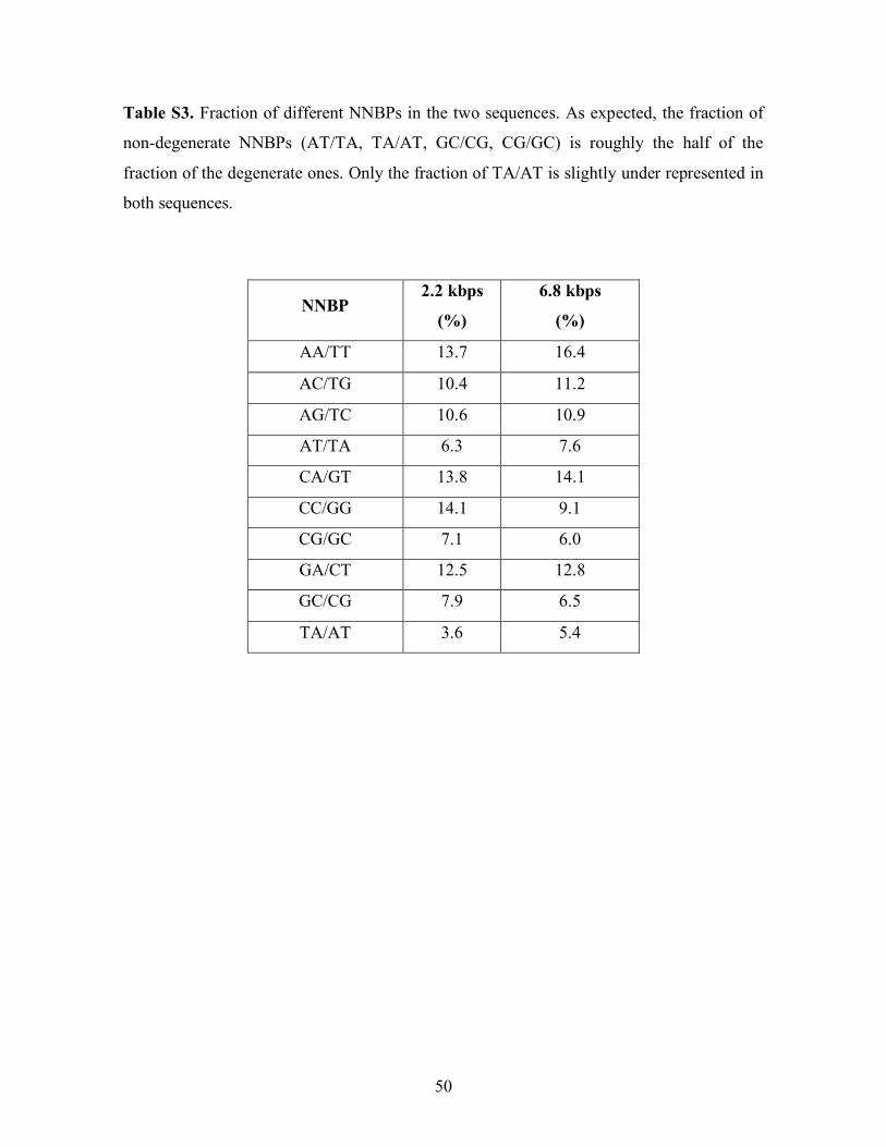
50

Table S3. Fraction of different NNBPs in the two sequences. As expected, the fraction of

non-degenerate NNBPs (AT/TA, TA/AT, GC/CG, CG/GC) is roughly the half of the

fraction of the degenerate ones. Only the fraction of TA/AT is slightly under represented in

both sequences.

NNBP 2.2 kbps

(%)

6.8 kbps

(%)

AA/TT 13.7 16.4

AC/TG 10.4 11.2

AG/TC 10.6 10.9

AT/TA 6.3 7.6

CA/GT 13.8 14.1

CC/GG 14.1 9.1

CG/GC 7.1 6.0

GA/CT 12.5 12.8

GC/CG 7.9 6.5

TA/AT 3.6 5.4

51

Table S4. Elastic parameters of ssDNA at different salt concentration. d is the

interphosphate distance for each model, lp is the persistence length of the WLC and b is the

Kuhn length of the FJC. The mean values were obtained after averaging over 5 molecules

for each salt, except for 25 mM and 100 mM that were averaged over 4 molecules and for

50 mM that were averaged over 3.

WLC model

d = 0.665 nm

FJC model

d = 0.59 nm

Salt [NaCl] lp (nm) b (nm)

10 mM 1.14 (0.1) -

25 mM 0.93 (0.1) -

50 mM 0.88 (0.1) -

100 mM - 1.37 (0.1)

250 mM - 1.25 (0.1)

500 mM - 1.20 (0.1)

1000 mM - 1.15 (0.1)