Single Image Depth Estimation via Deep Learning

Wei SongStanford University

Stanford, CA

AbstractThe goal of the project is to apply directsupervised deep learning to the problem ofmonocular depth estimation of still images.We have done experiments with two differenttypes of deep neural network architecture fordepth estimation, and performed regression onthe sparse coding of depths with appropriateobjective functions. Our best model achievedan average error in the ln space of 0.0891 forthe training and 0.26 for the testing set. Thispreliminary result demonstrates the feasibility ofusing deep neural network for still image depthestimation.

1 Introduction

Despite the fact that humans can easily infer the depths ofscenes presented in pictures, monocular depth estimationhas long been a difficult problem in computer visionresearch. This is mainly due to the fact that withouthigh level understanding of the real world, local appearancealone is insufficient to resolve depth ambiguities. So far,many of the state-of-the-art approaches apply probabilisticgraphical models to enforce local consistencies among thedepth pixels and apply some other high-level informationfor resolving ambiguities. Some recent research doneat Stanford such as the one described in [1] appliedsuper-pixel-based Markov Random Field (MRF) whileusing a predefined-set of semantic labels (e.g. sky, tree)as the prior for the depths; in [2], the authors also appliedMRF and incorporated the likelihood of the 3D structureof the scenes.

In this project, we take a different approach bydirectly performing training on the whitened images whileusing some representation of the depths as the labelswithout introducing any other features or prior knowledge.Specifically, we will be using deep neural network for thistask. Deep neural networks have shown great potentialin many computer vision applications such as the winningmodel in the 2012 LSVRC contest for image classification[3]. Such impressive results demonstrate deep learning’scapability of capturing high level concepts entirely fromthe images. Therefore, it is likely that it can also resolvedepth ambiguities when trained with sufficient amountof data. Another motivation for this project is for usto experiment training a shared network for both depth

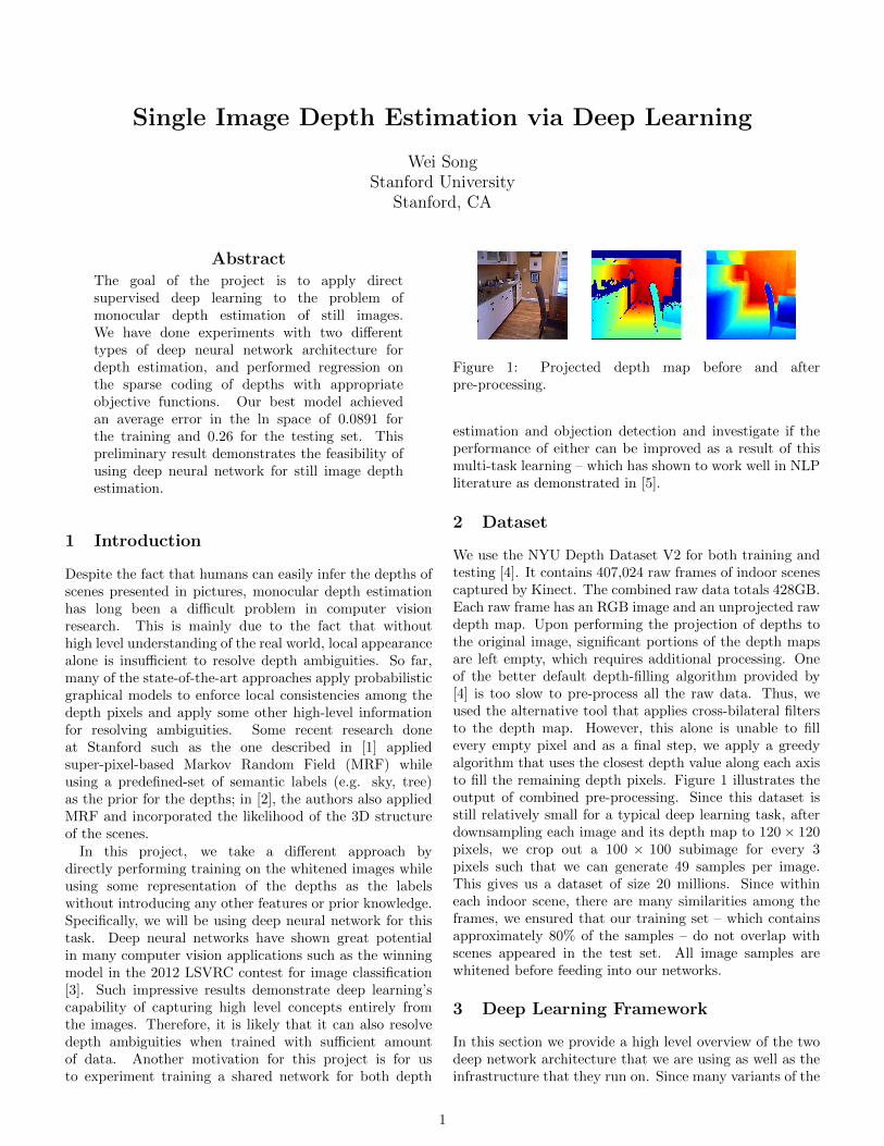
Figure 1: Projected depth map before and afterpre-processing.

estimation and objection detection and investigate if theperformance of either can be improved as a result of thismulti-task learning – which has shown to work well in NLPliterature as demonstrated in [5].

2 Dataset

We use the NYU Depth Dataset V2 for both training andtesting [4]. It contains 407,024 raw frames of indoor scenescaptured by Kinect. The combined raw data totals 428GB.Each raw frame has an RGB image and an unprojected rawdepth map. Upon performing the projection of depths tothe original image, significant portions of the depth mapsare left empty, which requires additional processing. Oneof the better default depth-filling algorithm provided by[4] is too slow to pre-process all the raw data. Thus, weused the alternative tool that applies cross-bilateral filtersto the depth map. However, this alone is unable to fillevery empty pixel and as a final step, we apply a greedyalgorithm that uses the closest depth value along each axisto fill the remaining depth pixels. Figure 1 illustrates theoutput of combined pre-processing. Since this dataset isstill relatively small for a typical deep learning task, afterdownsampling each image and its depth map to 120× 120pixels, we crop out a 100 × 100 subimage for every 3pixels such that we can generate 49 samples per image.This gives us a dataset of size 20 millions. Since withineach indoor scene, there are many similarities among theframes, we ensured that our training set – which containsapproximately 80% of the samples – do not overlap withscenes appeared in the test set. All image samples arewhitened before feeding into our networks.

3 Deep Learning Framework

In this section we provide a high level overview of the twodeep network architecture that we are using as well as theinfrastructure that they run on. Since many variants of the

1

Input

FilteringPooling

LCN Output

Figure 2: An illustration of one of the layers of RICA

networks have been experimented, the descriptions here arekept as generic as possible.

3.1 RICA Network

This architecture is similar to Google Brain’s unsupervisedlearning network as described in [6]. In a nutshell, eachlayer in the network contains three sub-layers: a localreceptive filtering layer where each neuron connects to asub-region of its input layer, a pooling layer that whereeach neuron computes some non-linear function of theinput field, and a Local Contrast Normalization (LCN)layer as shown in Figure 2. Typically, two or threesuch layers are stacked together followed by an outputlayer. We perform direct supervised learning (or finetuning) on the data without unsupervised pre-training.The output layer is also different as it will be discussedlater. Other hyper-parameters such as the input size,filtering size, number of depths maps, pooling sizes andpooling strategies also vary.

3.2 Krizhevsky’s Network

This is also known as the ”Drednet”. One of thekey differences between the RICA and the Krizhevsky’snetwork is that unlike RICA, the filters are allconvolutional. That is, the weights of the filters in eachlayer are tied. This significantly reduces the number ofparameters need to be learned per map, which allowsa higher number of maps generated at each layer [3].The layers of Krizhevsky’s network is not as orderedas RICA’s mentioned earlier. The first five layers aremixed combination of pooling, LCN and filtering layers ofvarious sizes, while the remaining two layers are denselyconnected layers. Another important aspect of Drednetis the activation unit. Typically, a smooth differetiablefunction such as the sigmoid or tanh functions are usedfor activation. In Krizhevsky’s network, Rectified LinearUnits (ReLUs) are used, which simply takes the maximumbetween the input and 0. Unsurprisingly, ReLUs are veryefficient, and in fact yield better results for many visionrelated tasks [3]. One regularization technique applied israndom dropouts, which randomly omits neurons duringtraining such that the dependencies among neurons arereduced. We use this network as the baseline and tweakmany of the hyper-parameters for experiments.

0 0.1 0.2 0.30

0.05

0.1

0.15

Sparsity

Ave

rage

Logge

dE

rror

Figure 3: Average absolute error in log space forreconstruction vs the sparsity (i.e. percentage of non-zerovalues of the embeddings) by varying β

3.3 Infrastructure

All of the training and evaluation of the deep networks aredone using the distributed GPU infrastructure as describedin [7]. At a high level, each machine has 4 high-end GPUs,and the intercommunication between the machines rely onInfiniBand to match the desired throughput. Most of thenetworks used in this project uses 1-2 machines or 2-8GPUs. The configurations of the networks are written inPython, but at the low-level, most of the computationalintensive tasks are written in CUDA. MPI is used tocoordinate the workers.

4 Sparse Coding of Depths

Initially, we defined our objective function as the squaredL2 norm between the logged depth values and theprediction. However, we obtained very poor results forboth RICA and Krizhevsky’s networks. In particular, itseems that neither of the two networks is learning the rightobjective as shown in Section 6. Thus, we decided to changeour representation of the depths. Instead of asking thenetwork to predict the logged depth values for every pixel,we encode the depth maps through sparse coding such thateach depth map is represented as four vectors where eachvector represents the sparse embedding of a quadrant of thedepth map. We used the method and code as described in[8]. The variant of sparse coding we used can be formulatedas follows,

minimizeB,S1

2σ2‖X −BS‖2F + β

∑i,j

‖Sij‖1

subject to∑i

B2ij ≤ c, ∀j = 1, ..., n

where X is the original data, B is the dictionary, and Sis the sparse representation. Holding either B or S fixedmakes the problem convex, but it’s not convex when bothcan be optimized. The authors in [8] proposed an efficientalgorithm that alternates the optimization of B and S whileholding the other variable fixed.

2

Figure 4: Image on the far left is the ground truth. β = 1, 0.1, 0.01, 0.001 are used for the four reconstruction. Thesparsities of their representations are 1.5%, 5.2%, 14%, 28%, respectively.

Figure 5: Our 512-basis sparse coding dictionry learnedfrom 4 miilion 20× 20 depth patches.

For our dataset, we downscale each jittered depth mapto 40 × 40. We are willing to downsample to such smallscale because the texture in depth maps are relativelylow compared to typical images. We then subtract apreviously computed mean of all downsampled depth mapsand break it down into four 20 × 20 patches – one foreach quadrant. For each patch, we encode it using thedictionary that we learned from approximately 4 millionpatches generated in a similar fashion. Figure 4 illustratesthe effect of varying the L1 regularization constant β, whichregulates the amount of sparsity during reconstruction.Note that permitting higher sparsity yields almost a perfectreconstruction of the downsampled ground truth depth asshown in figure 3. For our problem, we use β = 0.1,which yields an average sparsity around 5% and 0.04average logged difference for all the patches. This strategytransforms the representation of each depth map of ajittered image to a vector of size 2048 with approximately100 non-zero values when using a sparse dictionary size of512.

The reason we use sparse coding over other methods suchas PCA is that sparse coding allows over-complete basis,which gives more expressive power to the dictionary whilemaintaining low sparsities. Our learned dictionary of size512 is shown in Figure 5. Note that this may look differentfrom a typical dictionary learned on whitened images. Oneof the reasons is that in order to reconstruct the original

Models Avg L2 logged Test ErrKrizhevsky’s baseline 3.12No Dropout 3.24Three 2048 dense layers 3.08

Table 1: Some failed but saved results of models based onKrizhevsky’s network not using sparse coding.

Labels

Predicted

Figure 6: Poor results when not using sparse embedding aslabels. Vast majority of the output by both networks didnot resemble any pattern of the target labels.

depth map, the dictionary must retain the depth valueswithin the basis vectors. As a result, there aren’t as manypatches with mostly gray regions.

5 Objective Function

Using sparse coding to represent the depth maps posesanother problem: since the representations are very sparse,when using the common choice of L1 or L2 norm as theobjective function, the networks often learn to outputpredictions close to the zero vectors – which in fact doproduce very low objective values because we subtract alldepth maps by a mean depth map. This is especially thecase for RICA network. Inspired by a very recent paperas described in [9] where the authors of the paper faceda similar problem when using 0-1 vector to represent thepresence of objects, we attempted to fix this issue by usingthe following objective function

minΘ

∑i

∥∥∥(Diag(1{s(i) 6= 0}) + λI)1/2(hΘ(x(i))− s(i))∥∥∥2

2

Here, s(i) is the sparse vector of size n representing theembedding of the depths of the i-th sample. The indicatorfunction converts s(i) to {0, 1}n such that a field in theoutput is 1 if and only if the corresponding field in s(i)

is non-zero. Thus, by using smaller values of λ, we are

3

Training set Test set

Sparse Encoded

Estimated

Figure 7: Results obtained using our best model. First columns of each dataset are depths maps that achieved very lowerror, while the fourth one has very high error.

Model and Obj Function SC MSE Train SC MSE Test Abs log Train Err Abs log Test ErrRICA, λ = 0.001 0.0986 0.108 2.588 2.641RICA, λ = 0.01 0.0718 0.0847 1.290 1.221RICA, λ = 0.03 0.0380 0.0574 0.781 0.788RICA, λ = 0.05 0.0364 0.0557 0.724 0.737RICA, λ = 0.07 0.0457 0.0577 0.825 0.819Drednet, λ = 0.05 0.0461 0.0515 1.105 1.089Drednet, λ = 0.1 0.0280 0.0404 0.631 0.652Drednet, λ = 0.5 0.0144 0.0313 0.211 0.327Drednet, L2 0.0210 0.0366 0.246 0.379Drednet, Varying Obj 0.0127 0.0276 0.0891 0.260

Table 2: Results for models that produced non-zero outputs. Here, SC is the mean squared error of sparse code, and theabsolute log errors are absolute average absolute difference between each depth pixel in ln space. The best model wasproduced by increasing λ during training and then switching to L2 near the end.

effectively putting more relatively weights on the non-zerofields of the sparse vector, which in turn penalizes thenetwork for outputting zero vectors. As λ approachesinfinity, this is analogous to the squared L2 objectivefunction. Note that the indicator function can be replacedwith any other non-negative functions. In particular, wetried to use the absolute and squared values of the sparsevectors. However, they did not prevent the network fromoutputting near zero vectors, and we believe the mainreason is that many of the non-zero values in the sparserepresentation are relatively small. Thus, when using thesevalues as the relative weights, most values still have thesame penalization as compared to the zero fields.

6 Early Results

As mentioned earlier, the results for directly estimatingthe logged values of the depth maps have been quitepoor. Due to a disk failure in AI Lab in late October,much of the evaluations of those models and our inputdata is lost, and everything has to be re-downloaded andre-processed. Since we’ve decided to use sparse coding asour new representation and re-running the experiments arerather expensive, we did not go back and prepare the olddata input again to regenerate those models. However,we do have some saved results demonstrating the poorperformance of those models and justifying why we havedecided to switch to sparse coding. Table 1 shows theresults of some variations of the Krizhevsky’s network.Note that the actual number of models tested far exceedswhat’s shown here, but the evaluation data is lost and none

had been able to achieve any reasonable output. Figure 6also shows some randomly sampled saved outputs by bothRICA and Krizhevsky’s network. Clearly, We can observethat depths estimation is not being properly learned at allwhen performing regression on the labels directly – at leastfor all the models we’ve experimented.

7 Results with Sparse Coding

Using sparse coding to represent the depths and with thenew objective function we defined earlier, we are finallybe able to obtain some models that can begin to estimatereasonable depth maps for images in both training andtesting dataset. Figure 7 shows some good and bad outputproduced by our best models. Despite that our models stillhave trouble estimating the depths of more complex shapes,they can capture the basic structures of many differentscenes. It’s worth noting that even though each quadrant isrepresented by a separate sparse vector, the network is ableto produce embeddings that generate smooth boundariesbetween the quadrants for most samples.

Table 2 shows a subset of models we tried bychanging the objective function and other appropriatehyper-parameters. Note that we did not include theoutcome of models that output results close to the zerovectors. The reason being that although numericallytheir errors are comparable to the models we’ve shown,qualitatively speaking, they tend to generate the samedepth map for most images, which is an unacceptablebehavior. For the RICA networks, we used map size 8and filter size 10 with 2 stacked layers. For Krizhevsky’s

4

0 20 40 60 80 100

0

1

2

3

4

5

Sorted Index

Ab

solu

teC

oeffi

cien

tGround Truth

RICA, L1

RICA, L2

RICA, λ = 0.1

RICA, λ = 0.05

Drednet, λ = 0.05

Drednet, λ = 0.5

Drednet Varying Obj

Figure 8: Absolute values of the largest 100 coefficientsin the sparse representation of each model sorted indescending order.

network, we used filter size of 12, 5, 3, 3, and 3 for the first5 layers with max-pooling on the 1st, 2nd and 5th. Thepooling size used is 2. The last two dense layers each have4096 neurons, and the number of maps for the first 5 layersare 100, 260, 384, 384 and 256. The initialization of bothnetworks are models trained for the image classificationtasks. Our results show that Drednet performs better thanRICA, which is unsurprising due to the larger number ofparameters used in Drednet. Relatively speaking, our newobjective function seems to make very significant impact onthe RICA network. In particular, using λ value that’s closeto the average sparsity of the embeddings produced the bestmodel. However, this isn’t the case for Drednet and usinglarger λ values seem obtains better results. Our best modelwas trained by modifying the Drednet’s objective functionfrom low λ = 0.05 to 0.5, and then switched to squared L2

as training progresses. This indicates that the initializationof the networks for different objective function impacts theconvergence of the networks.

Since our network outputs the sparse coding of thequadrants of the depth map, it is also interesting to analyzethis output before decoding them to depths values. For afixed random scene, by taking the absolute values of thecoefficients of the sparse representation then sorting themin descending order, we obtained Figure 8, which displaysthe largest 100 coefficients for each model. While this maynot be representative of all embeddings, we can observesome expected trends. Both L1 and L2 for RICA producedembeddings that are very close to the zero vectors, andsmaller λ values for both networks result in a fatter tailcompared to the larger λ values.

8 Conclusion and Future Work

Our project has demonstrated the feasibility of using deepneural networks to directly estimate the depth valuesof single still images without using any hierarchical orhand-engineered features. Our best models are able to

estimate reasonable depth maps for most scenes in trainingand testing set.

There is certainly room for further improvements. Dueto the long training time and resource required for eachmodel (e.g. Drednet needs 8 GPUs and days to converge),we weren’t able to experiment the effect of varying toomany hyper-parameters as we’d like to but they shouldalso be tried in the future. We are also consideringturning off max-poolings since we may not actually wantthe translation invariance offered by it for this particulartask, though this would require even more VRAM andGPUs to hold the network.

The relatively large difference between the training andtesting error suggests overfitting of the training data.There are several ways to remedy this. One is to furtherdownsample the output space or use smaller dictionary forsparse coding. Alternatively, we could also introduce moredropout and regularization in out networks. The effect ofvarying the objective function during training should alsobe further analyzed and tested with more trials on differentmodels.

Acknowledgement

I’d like to thank Stanford’s Artificial IntelligenceLaboratory for providing me with the necessary machinesand tools to carry out large-scale deep learning.Specifically, I’d like to thank Brody Huval for guidingme throughout the entire project. He has also helpedpre-processing the NYU dataset, helping me setting upinitial experiments and making necessary changes to thecodebase for the depth prediction task. I’d also like tothank Adam Coates for continuously providing feedbackon our results.

References

[1] B. Liu, et al. “Single image depth estimation from predictedsemantic labels.” CVPR 2010.

[2] A. Saxena, Ashutosh, et al. “Make3D: Depth Perceptionfrom a Single Still Image.” AAAI 2008.

[3] A. Krizhevsky, et al. “Imagenet classification with deepconvolutional neural networks.” NIPS 2012.

[4] N. Silberman, Nathan, et al. “Indoor segmentation andsupport inference from RGBD images.” ECCV 2012.

[5] R. Collobert and J. Weston. “A unified architecture fornatural language processing: Deep neural networks withmultitask learning.” ICML 2008.

[6] Q.V. Le, et al. “Building high-level features using large scaleunsupervised learning”. ICCV 2012.

[7] A. Coates, et al. “Deep learning with COTS HPC systems.”ICML 2013.

[8] Lee, Honglak, et al. “Efficient sparse coding algorithms.”NIPS 2006.

[9] C. Szegedy, et al. “Deep Neural Networks for ObjectDetection.” NIPS 2013.

5