simultaneous orbit and atmospheric density estimation for

1

American Institute of Aeronautics and Astronautics

Simultaneous Orbit and Atmospheric Density Estimation for

a Satellite Constellation

Joanna C. Hinks* and Mark L. Psiaki

†

Cornell University, Ithaca, NY 14853

A method is defined for simultaneous atmospheric density calibration and satellite orbit

determination for a satellite constellation, and a linearized observability analysis is

performed to evaluate the feasibility of the approach. Such an estimation scheme will

provide data-based estimates of upper atmosphere density that improve on existing models,

e.g. the Jacchia models, along with enhanced accuracy of the associated satellites’ orbits. A

new spline-based atmospheric density parameterization is developed that meshes well with

the structure of the orbit determination problem and can be initialized so as to match the

outputs of a traditional model. While conceptually similar to previous atmospheric

calibration efforts, the proposed constellation approach restricts its global density estimates

to the relevant satellite altitude range and thus reduces the complexity of the estimation

problem. Measurements include dual-one-way-ranging between pairs of adjacent satellites

in the same orbital plane, and carrier phase and pseudorange measurements between

ground stations and satellites. Equations for a linearized observability analysis are derived

and shown to be equivalent to the covariance calculations of an extended square-root

information filter. In addition to the system observability evaluation, the impact of

incorporating some a priori density information is explored. The results show that

atmospheric density can be observed, but a reasonable amount of a priori information is

necessary to obtain useful estimates. Degree of observability depends on the constellation

configuration and dynamic model parameter values.

I. Introduction

RBIT determination is the process by which satellite trajectories are estimated. The available measurements

are combined to yield a history of the satellite’s position and velocity. Accuracy of orbit estimates is limited by

the quality, quantity, and types of available measurements, and by the accuracy of the dynamic model assumed for

the satellite’s motion. Thus if an application requires high precision, one normally needs high quality measurements

and models.

For many satellites in low earth orbit (LEO), the largest dynamic model uncertainty stems from atmospheric

drag1. Acceleration due to atmospheric drag is related to atmospheric density by the equation

(1)

where is a drag coefficient, is the cross-sectional area of the satellite in the direction of travel, is the

total spacecraft mass, is the velocity magnitude relative to the ambient atmosphere, and is a unit vector in the

relative velocity direction. Uncertainty enters this equation in three ways. First, the scalar product

, known

as the inverse ballistic coefficient, is generally uncertain and may be time-varying. Second, the relative velocity

may be uncertain, either because it has not yet been estimated accurately or because the local wind does not rotate

perfectly with the Earth. Finally, atmospheric density is very difficult to determine. Three basic paradigms exist for

dealing with drag uncertainty: It can be modeled, measured directly or indirectly, or estimated in conjunction with

satellite orbits.

* Ph.D. Candidate, Sibley School of Mechanical and Aerospace Engineering, 127 Upson Hall, Student Member,

AIAA. † Professor, Sibley School of Mechanical and Aerospace Engineering, 206 Upson Hall. Associate Fellow, AIAA.

O

AIAA Guidance, Navigation, and Control Conference2 - 5 August 2010, Toronto, Ontario Canada

AIAA 2010-8258

Copyright © 2010 by Joanna C. Hinks and Mark L. Psiaki. Published by the American Institute of Aeronautics and Astronautics, Inc., with permission.

2


Models of atmospheric density have been developed and studied widely in the past 50 years. The Jacchia series

of models assumes a temperature profile, and integrates the barometric and diffusion differential equations upwards

to the desired altitude. A number of empirical corrections are also applied based on satellite orbit data 2,3,4,5

. The

Mass Spectrometer and Incoherent Scatter (MSIS) series of models has been derived based on data from science

instruments. This series simultaneously computes temperature and density by evaluating a complicated set of

functions involving hundreds or thousands of coefficients 6,7,8

. While these two series of density models are the

most common, many others have been developed by various researchers. All of them, however, retain fairly large

levels of uncertainty even after decades of development. Typical model standard deviations start at 10-20% under

normal conditions and can be much greater at times of unusually high or low solar and geomagnetic activity 9,10,11

.

Much of this inaccuracy comes from the inadequacy of currently available metrics of solar activity, which do not

fully capture the effects of the sun on the atmosphere 12,13

. Most models take as inputs the 10.7 cm solar flux

and the 3-hourly geomagnetic index (or its equivalent ), which are reasonable but incomplete metrics.

Furthermore, there is still a great deal to be learned about the complex dynamics of the atmosphere, and good

measurements are a limiting factor. It is unlikely that modeling efforts will improve significantly in the near future.

The second approach to the atmospheric density problem depends on highly accurate measurements or targeted

sensors to remove the effects of atmospheric drag from the orbit solution. For instance, satellite missions like

CHAMP and GRACE carry high-quality accelerometers to estimate non-gravitational perturbations 14

. Special

sensors on Dynamics Explorer 2 made in situ measurements of temperature and atmospheric composition, which

were later used to develop the MSIS models 15

. Increasingly, new satellite missions carry GPS receivers, which

support tracking of satellite motion to within centimeters and thus reduce or eliminate the need for accurate models

of dynamic perturbations 16

. There are even a few missions, such as Gravity Probe B, which eliminate drag

perturbations entirely by flying a proof mass in a vacuum chamber and actively steering the spacecraft to follow its

drag-free motion 17

. While all of these techniques are effective, they can be implemented only with expensive,

dedicated, space-born instrumentation.

When atmospheric models are not sufficiently accurate and special flight instruments are not an option, one can

attempt to estimate satellite drag or density parameters along with the orbits. In particular, atmospheric calibration

efforts attempt to estimate global density parameters or density corrections on the basis of some form of satellite

data. The density estimates can then be applied to the orbits of other spacecraft as well. Several calibration projects

have recently demonstrated improved density knowledge and orbit determination performance in comparison with

standard models. For example, some approaches take as their measurements the two-line elements (TLE’s) of

tracked space objects, which are made available by NORAD, and employ long histories of these measurements to

calculate corrections to a density model 18,19,20,21

. Another method’s calibration strategy aims to reduce the standard

deviation of many months’ worth of multi-day batch fits of a satellite’s inverse ballistic coefficient 12,13

. The Air

Force Space Battlelab has developed the High Accuracy Satellite Density Model (HASDM), which incorporates

Space Surveillance Network (SSN) data from a set of frequently tracked calibration satellites to both estimate and

predict global atmospheric density 22,23

. All of these methods have shown promise in reducing orbit determination

fit errors for satellites not included in the calibration set.

This paper proposes a new form of atmospheric calibration to support precision orbit determination for a satellite

constellation. Its approach attempts to simultaneously estimate the satellite orbits along with the density profile for

the altitude region spanned by the constellation. It employs the preexisting radiocommunication signals of the

constellation as its measurements, rather than dedicated tracking data. Significantly, none of the signals were

designed for navigation, yet the information in the data set exceeds what has typically been available for density

estimation.

The candidate constellation would have 50-100 satellites arranged in several evenly spaced orbital planes, with

nearly circular, low-earth orbits. Each satellite in an orbital plane would encounter similar density variations to

those experienced by the others in that plane, thus providing a multiplicity of measurements for a given density

feature. Adjacent satellite pairs would be joined by crosslink range signals, and additional signals would measure

ranges between the satellites and a set of ground stations. For the envisioned system, sub-meter orbit accuracy is

desired throughout the orbit, so the density must be parameterized in a way that provides sufficient spatial and

temporal resolution 24

. A spline-based density parameterization method has been developed for this purpose.

The goal of this paper is to study the proposed atmospheric calibration/orbit-determination scheme, particularly

with respect to observability. Specifically, it seeks to answer the question, “Is the available data sufficient to

simultaneously estimate the orbits of all satellites in the constellation, as well as the atmospheric density spline

parameters?” One would not expect the system to be fully observable, due to the large number of parameters to be

estimated and due to coupling of certain parameters’ effects. However, this estimation scheme can be used in a

recursive (Kalman) filtering context, where a priori estimates are available from physics or past efforts. In such a

3


scenario, an observability analysis can still yield information about which parts of the a priori estimate can be

improved with new data and which quantities should be more carefully modeled because the measurements add no

further knowledge.

This paper offers three main contributions. First, it develops a spline-based density parameterization method

which is well-suited to the constellation estimation context. Second, it defines and elaborates the problem of

performing atmospheric calibration using a constellation of satellites. Finally, a linearized observability analysis is

performed to determine the feasibility of the proposed approach and to identify potential areas of weakness.

The rest of this paper is organized as follows: Section II gives an overview of the spline-based density

parameterization technique and some of the issues related to representation of density. In Section III, the proposed

estimation problem is formulated, and important assumptions about the dynamics and measurements of the system

are clarified. Section IV considers the issue of observability, and derives the equations for the linearized

observability analysis. Results of the observability analysis are given in Section V along with some suggested

alternative tests and their results. Section VI presents the paper’s conclusions and suggests areas for future study.

II. Spline-Based Density Parameterization

In order to estimate an atmospheric density distribution, one must first decide how to represent it. This choice

will guide the development of the estimation scheme. Some past efforts have used altitude-dependent corrections to

the outputs of a Jacchia model 19

. Another parameterization makes corrections to the model inputs, for instance by

specifying the coefficients of a spherical harmonic expansion for exospheric temperature 22

above. The chosen

method must be capable of representing a complex density distribution and be appropriate for the specific purposes

in mind.

The chosen parameterization takes the form

(2)

In this equation, the inputs are latitude , longitude in a sun-fixed frame (essential the angular form of local solar

time), altitude , and a parameter vector , with and defined relative to an ellipsoid. For each latitude and

longitude, density has a value at a nominal altitude , and above and below this nominal altitude it varies

exponentially according to the scale height . Both and are splined functions of latitude and

longitude. The parameter vector stores the values (and spatial derivatives) of and at particular grid

points, and cubic spline interpolation is used to ensure smooth variation between these points. Given a suitable

number of grid points, this parameterization will be comparable to a spherical harmonic representation. It has been

chosen because of the ease with which various of its partial derivatives can be calculated. A detailed description and

equations of the spline interpolation, as well as other aspects of this parameterization, are given in the appendix at

the end of this paper.

It is widely recognized that Earth’s atmosphere is only approximately exponential in density. This exponential

assumption is valid, however, over a small range of altitudes. For the nearly-circular orbits of a candidate satellite

constellation, the altitudes encountered fall well within the acceptable range. This has been verified by determining

altitude variations resulting from both actual satellite orbit eccentricities and the effects of Earth’s ellipsoidal shape.

Within the determined range, evaluations of standard atmospheric models such as NRLMSISE-00 8 show density

variations that are practically indistinguishable from the exponential form. Because this parameterization is

specifically intended for a satellite constellation application, it does not need to represent densities of the full

atmosphere; a thin shell at the right altitude is adequate. The nominal altitude falls approximately in the

center of this shell, and its latitude dependence adjusts for the curvature of the WGS-84 ellipsoid relative to the

nominal constellation altitude.

A natural way to visualize the spline-based density parameterization is as a two-dimensional Cartesian grid of

points in the variables , with a surface stretched between them. As countless historical mapmakers can attest,

a number of mathematical difficulties arise from the representation of a sphere as a rectangular grid. For instance,

the mapping is not one-to-one; when one reaches the far “eastern” edge of the grid, where , this is really

the same location as the corresponding point on the “western” edge, where . At the poles, the situation is

further complicated because, regardless of the longitude, every point with represents the “North pole”, and every point with represents the “South pole”. These singularities give rise to a number of constraints on the valid node point values of the spline parameterization. Other constraints are entailed by the physical

4


requirement that the density vary “smoothly” over the globe, including at the poles. This second group of

constraints influences the spatial derivative values that are also stored as part of the parameterization. The appendix

contains further details of the constraints and their implementation.

All the density information at the constellation altitude can be captured by the values in the parameter vector ,

along with the spline algorithms that extract and from . As described above, the

information stored in this vector is a list of density and scale height values at certain points, and also the first

partial derivatives of those values with respect to latitude and longitude and the cross-partial-derivative with respect

to both latitude and longitude. Thus, there are eight scalar pieces of information for each distinct point: Four

associated with density,

, and four associated with scale height,

. These values are all stacked together to form the vector . Although the order of the elements might

change, a segment of this vector would look like

(3)

for a general grid point that is not at one of the poles.

The length of the parameter vector is determined by the number of latitude and longitude grid points, that is, the

desired resolution of the estimated density field. Typically, there are 150 to 300 scalar parameters to be estimated.

While this number may seem high, it is manageable. A satellite constellation may have close to 1000 values to be

estimated just for the satellite orbital states and a few satellite-specific parameters. Therefore, an extra 200

atmospheric density parameters may be reasonable.

A second concern for a large number of atmospheric parameters, and the main topic of this paper, is that of their

observability. Even with incomplete observability an operational filter could still function well. A recursive

estimator would start with some a priori information on density and improve on that initial guess. It would leave

unobservable parameter combinations at their a priori values.

While the preceding description explains how a global density field can be stored, it provides no connection,

theoretical or empirical, to the physics of the atmosphere. Even if the estimation technique does not require an

initial guess, one desires some reassurance that results are realistic. Furthermore, nonlinear problems require a

sufficiently close initial estimate in order for linearization to be valid. These needs are met by an initialization

procedure that accepts any set of density “truth” data and outputs a corresponding vector . “Truth” data can come

from standard atmospheric models, or from satellite-carried sensors or any other source, as long as the density data

points are globally distributed. In order to estimate scale heights, some altitude diversity within the range of interest

is necessary. After one chooses the desired latitude and longitude resolution, the initialization procedure performs a

least-squares fit to find the values that most nearly cause the interpolated spline to match the data points. This

strategy has been found to fit “standard” density models closely with surprisingly few latitude and longitude

divisions.

5


For instance, Figure 1 shows a fit

of a splined parameterization with

five latitude points and six longitude

points. The fit is to the NRLMSISE-

00 model, during average solar and

geomagnetic conditions. The

surface is the cubic-spline-

interpolated manifold corresponding

to the solved-for parameters, and

the points are the model’s “data”.

For this particular fit, the mean

density relative error between the

data and the splined

parameterization was 0.51%, and the

maximum relative error was 4.22%.

This fit involves only 156

parameters and fits 3000 data points.

Note: Figure 1 depicts the splined

density only at the nominal altitude.

Its displayed data points are

artificially mapped to that altitude

by means of the splined scale height.

In order to use a particular

density parameterization for

estimation, one must be able to

derive its partial derivatives with respect to the elements of the filter’s estimated state. The partial derivatives

provide information about the way small changes in one quantity affect some other quantity of interest. For this

scenario, estimation requires the partial derivatives of density with respect to the inertial position vector (x, y, z

position, not , , position) and with respect to the parameter vector . Derivatives of the spline-parameterized

quantities and with respect to , , and the elements of can be computed using minor modifications of

the interpolation algorithm. Thus the quantities

,

,

,

,

, and

are readily available.

The desired partial derivatives

and

are then computed by some simple calculations and repeated

application of the chain rule. The appendix elaborates further on this topic for the interested reader.

III. Formulation of the Estimation Problem

The problem of determining satellite orbits and atmospheric density parameters from noisy data falls within the

scope of estimation theory. Estimation is the process by which one extracts desired information from measurements

in some optimal fashion. To employ standard estimation algorithms, two sets of mathematical models must be

created. First, there are differential or difference equations that model the dynamic process of interest. These

equations describe the evolution of the system state vector, where the states are the quantities to be estimated, such

as position, velocity, or time-varying parameters. Second, estimation methods need mathematical models of the

measurements, and specifically of the functional relationship between the state vector and the measurements. A

final requirement is a statistical description of all uncertainties in the system. The dynamics models include a

stochastic contribution from process noise, and the measurements models typically have additive noise

representative of sensor errors. Any correlations between process and measurement noise must be accurately

described.

A. State vector and dynamics models

The state vector for this estimation scheme contains many components. First, there are ten states associated with

each satellite. For the satellite, they are contained in the vector , which will be discussed in more detail below.

In addition to states relating to individual satellites, the state vector includes the atmospheric density parameter

vector , which will also be estimated. The last part of the state vector contains a set of “nuisance states” that must

Figure 1. Density initialization data from NRLMSISE-00 and the

corresponding best-fit splined surface

6


be estimated but are not actually of interest. These are unknown real-valued biases on accumulated delta range

phase measurements, and include two distinct sets of biases: and . The vector contains biases on

crosslink measurements between satellites, and contains biases on measurements between ground stations and

satellites. These measurement quantities are explained in more depth later in Section III. When all these states are

stacked, the dynamic state vector becomes

(4)

where is the full system state and is the number of satellites in the constellation. In its general form, the

nonlinear dynamics differential equation for this state vector can be written as

(5)

where defines the time evolution of all the states, and is the system process noise vector. The discretized

version of this function can be written as

(6)

where is the state at the sample time , and parameterizes during the interval from to . The

function is computed in practice via numerical integration of differential Eq. (5), starting from the

initial condition . The general function given in Eq. (5) can be broken down into specific functions for

the distinct components of the state vector.

Each individual satellite j has a set of states of the form

(7)

where is the satellite Cartesian position vector in an inertial frame,

is the corresponding velocity vector,

and are the satellite clock error and rate error, respectively, and

and

are the inverse ballistic coefficient

and the solar radiation pressure coefficient for that particular satellite.

Dynamic behavior for each satellite’s position and velocity is governed by Newton’s second law: acceleration is

proportional to force divided by mass. This leads to the equation

(8)

Note that no process noise enters the satellite dynamics directly. This analysis assumes that the dominant errors in

the dynamic model enter it through . The total force consists of summed contributions from Earth’s gravity,

the gravitational attractions of the Sun and Moon, atmospheric drag, and solar radiation pressure. A simplified Earth

gravity model with only a small number of terms will be used for this analysis. While additional forces and more

complicated force models would certainly be included in an actual orbit determination run, neglecting them here will

not significantly degrade the results of the observability analysis 25

.

7


In addition to its position and velocity dynamics, each satellite has dynamic models associated with its clock. A

standard clock error model is used 26

. It takes the form

(9)

where and

are phase and frequency process noise that drive the clock error. The statistical properties of the

process noise are chosen based on the particular type of clock carried by the satellite. These clock errors affect the

phases of the transmitted crosslink and downlink signals, and the crosslink receiver’s measured phase outputs.

Accelerations due to atmospheric drag and solar radiation pressure depend not only on environmental variables

but also on the shape, surface properties, and mass distribution of specific satellites. Generally, these effects are

captured by proportionality constants that multiply the relevant vector quantities. Both inverse ballistic coefficient

and solar radiation pressure coefficient

have dimensions of area divided by mass:

(10)

where and are the average projected areas perpendicular, respectively, to the velocity and sun directions.

The total spacecraft mass is , and and are nondimensional scalars. In situations where the projected areas

vary rapidly, a priori models of these variations, and , can be incorporated into the force models in

via the ratios and . Such models preserve the nearly constant nature of and

Due to the

remaining uncertainty, the states and

are modeled as either constants or slowly-varying random walks:

(11)

where and

are continuous time white noise for a random walk, or zero for constants. The joint observability

of these states and the atmospheric density states is a subject of investigation 27

.

After ten states for every satellite in the constellation, the system state vector contains a sub-vector of density

parameters. As the spline-based atmospheric density parameterization does not incorporate any physics, it is

difficult to say how its dynamics should be modeled. Empirically, the diurnal variation is the primary effect, but this

component has been removed by specifying the spline’s longitude grid relative to local solar time. Some diurnal

effects remain, however, due to rotation of the Earth-fixed magnetic field. Other well-documented variations

include effects of the 11-year solar cycle and the 27-day solar rotation period, variations due to specific solar

activity, variations caused by geomagnetic activity, a semiannual variation, and what are known as seasonal-

latitudinal variations 3. With the exception of the solar and geomagnetic activity effects, all of these components act

on much longer time scales than those envisioned for the estimation problem, and thus enter the problem mostly as

biases that would be included in the initialization procedure. One goal of this observability analysis is to determine

if the available data are sufficient to estimate the remaining short-term variations due to solar activity, geomagnetic

activity, and other random fluctuations.

In the absence of a reliable physics-based model for these effects, the dynamics of the density parameter vector

is modeled as a first-order Markov process, where each element evolves according to

(12)

where is the Markov time constant, is an a priori estimate of the element , and is the continuous

time process noise. Typically is the initial value determined from a fit to a standard model as in Figure 1.

Proper tuning of and the process noise intensity will prevent from reverting to the a priori standard model if

the data dictate otherwise.

8


Time constants for the process have been determined empirically from one of the standard models such as

Jacchia 71 or NRLMSISE-00. This was done by assuming different input histories to the model, representative of

mild, moderate, and severe solar and geomagnetic disturbances. For each set of inputs, the initialization procedure

yielded the corresponding , and the way in which the values in change with time was leveraged to select

appropriate process time constants and reasonable process noise intensities. Situations are considered where time

constants and process noise intensities can change over time in response to changes in geomagnetic or solar activity,

as described in Ref. 28.

In a typical batch observability analysis, process noise is neglected altogether in dynamic models, although its

effects may be characterized by studying the results of different batch interval lengths. If a relatively short batch

interval gives good observability, a higher level of process noise is acceptable. This paper incorporates process

noise directly, as will be explained in Section IV. The inclusion of process noise does not change the theoretical

observability of a system; rather, it provides a more realistic relative observability of the states.

The final part of the state vector contains all the measurement biases. Although their particular values are not

important, measurement biases must be estimated as part of the state vector in order to make optimal use of the

available accumulated delta range measurements. They are modeled as constants by the equation

(13)

The chief difficulty arising from the biases is their number. For every pair of adjacent satellites with dual one-

way ranging, there are two crosslink signals and distinct biases for each crosslink. Every time a satellite comes

within view of a ground station, a new bias from the resulting measurement gets added to the state vector. This bias

is constant for the entire pass of the satellite over that ground station, but if the ground station stops tracking the

satellite and then resumes tracking on another pass, a new bias applies to the measurement. Any satellite might pass

over any ground station any number of times, so the “obsolete” states in must be removed to keep the size

manageable.

B. Measurement Models

Estimation problems also require mathematical models of the way in which the system state affects the

measurements. These are necessary in order to optimally extract information about the system states from

measurements which are indirectly related to those states, noisy, or biased. Three types of measurements are

available for the proposed constellation orbit determination scheme. First, there are dual-one-way-ranging

measurements between the adjacent satellites in an orbital plane, called crosslinks. Each satellite of a pair measures

a phase-based accumulated delta range relative to the other satellite, with a unique unknown bias in each direction.

Next, there is an accumulated delta range between each ground station and every satellite it tracks at a given time.

This delta range also includes an unknown bias. Finally, there are GPS-like pseudorange measurements between the

ground stations and satellites. Although the pseudoranges are not biased, they are much noisier than the

corresponding accumulated delta ranges.

The crosslink measurements are formed as a beat phase: when a signal arrives from an adjacent satellite, its

phase is compared to the phase of the receiver satellite’s onboard oscillator. In this way it forms a biased range

measurement between the transmitting satellite’s position at the true time of transmission, , and the receiving

satellite’s position at the true time of reception, . Thus the equation for the crosslink accumulated delta range

between transmitting satellite and receiving satellite is given by

(14)

where is the accumulated delta range, converted to distance by the wavelength , is the position

vector of the receiving satellite at the true time of measurement, is the position vector of the transmitting

satellite at the true time of transmission, and

are the receiving and transmitting clock errors, respectively,

is the bias converted to an equivalent distance, and is noise. Delays due to neutral atmosphere are

nonexistent at satellite altitudes, and ionospheric effects are small.

9


While the physical measurement model is formed based on the positions at the true times of transmission and

reception, the receiver reports only the reception time according to its own internal clock, , and the transmitter

reports no time. This leaves the estimation algorithm the following challenge: It needs to use and as part

of the measurement model by which it estimates the state. These two times, however, must be inferred from state

vector elements. This inference is carried out by solving implicit constraint equations. Thus, there is a seeming

paradox of having to know the state in order to estimate it. One starts to resolve this paradox by considering the

implicit equations for and :

(15a)

(15b)

where

is the scalar range between the vectors and

, as in

the first term on the right hand side of Eq. (14). The first equation, Eq. (15a), is an implicit statement that receiver

clock time equals true measurement time plus the correction

that applies at . The second

equation constrains the reception time to equal plus the light travel time between satellite and satellite

.

Note that the functions ,

, and

are not standard components of a typical discrete-time estimation algorithm. They

assume that the estimation algorithm explicitly computes estimates of the states at sample times and . Recall

that these states are denoted by and . These non-standard functions are needed to interpolate the state

elements ,

, and

to the times and , because they normally differ from and . Any

reasonable interpolation algorithm should suffice.

The pair of constraints in Eqs. (15a)-(15b) can be solved iteratively for the true times and by means

of a Newton-Raphson approach. The effect is that and are implicit functions of and .

Substitution of these implicit functions into the right hand side of Eq. (14) yields a measurement model that

effectively depends only on and :

(16)

Extra care must be taken not to confuse

with

, with , and so forth. Although they apply to the

same pair of satellites, the roles of receiver and transmitter are not interchangeable in these equations.

The beat carrier phase measurement on the downlink from a satellite to a ground station is very similar to the

crosslink measurement in many respects. The measurements have the same general structure, and are biased in the

same way. Ground station clocks, however, are assumed to be disciplined by GPS, so that the clock error is

negligible. The resulting beat carrier phase between ground station and satellite is

(17)

in which most of the quantities are defined in ways analogous to those in Eq. (14). is the known ground

station location, which depends on time because it is given in inertial coordinates. While the true time of reception

is known here, the transmission time once again is not. A version of the second implicit constraint in Eq.

(15b) must be employed to resolve this problem:

(18)

10


where is the range that appears as the first term on the right hand side of Eq. (17).

Pseudoranges at the ground stations measure ranges to the same satellites as the corresponding beat carrier phase

measurements. They do not have any unknown bias, but their noise covariance is generally much higher than the

phase ranges. The pseudorange measurement equation takes the form

(19)

Once again the implicit constraint of Eq. (18) must be solved iteratively to determine the true time of

transmission of the signal. The problem of implicit measurement times is common to techniques that measure ranges

by calculating transmission delay. Readers interested in this topic are encouraged to refer to 29

.

No terms are included for the ionosphere or neutral atmosphere in the carrier phase and pseudorange

measurement models, and this omission is intentional. It is assumed that these components can be modeled well

enough to be corrected and removed from the ground-based measurements. Work is ongoing in this area. It includes

efforts to use dual-frequency GPS measurements of TEC, available at ground stations, to create a local model of the

ionosphere 30

.

Each of the three measurement models takes the generic form

(20)

where is the scalar error for this measurement. This equation presumes solution for the implicitly defined times

and and substitution of these solutions into the measurement models as in Eq. (16) for the crosslinks

case. A carrier phase version of Eq. (16) can be developed from Eq. (17) and a pseudorange version from Eq. (19).

Typically, multiple measurements will occur in the sample interval . That is, and

for each such measurement. (The rare measurements that overlap two sample intervals can be

discarded for the sake of simplicity.) All these measurements and their corresponding model functions can be

stacked to form the vector measurement equation

(21)

This is the general, but non-standard, form that will be used in this paper’s observability analysis.

IV. Derivation of the Observability Analysis Equations

Conceptually, a system is observable when it is possible to uniquely determine the initial state of the system

from some finite number of measurements. In the field of estimation, it is often useful to know whether a given

system is observable before making a possibly futile attempt to estimate its state. That is the main idea behind this

paper: to study whether it is theoretically possible to determine atmospheric density and the orbits of a satellite

constellation, given the proposed measurements. A closely related concept is constructability, which asks whether

the measurements are sufficient to uniquely determine the final state, as opposed to initial state. The conditions are

mathematically equivalent in cases, including the current case, where the system dynamics are invertible. For this

reason this paper will continue to use the terminology observability analysis, although technically it performs a

constructability analysis due to constructability’s closer connection with the standard filtering problem.

If a system is linear, then it either is or is not observable. For nonlinear systems, however, it may not be possible

to make such a clear distinction. Asking whether a system is observable is equivalent to asking whether a cost

function based on measurement error residuals has a global minimum. Many nonlinear systems have a distinct

global minimum, but may also have additional distinct local minima. This paper examines the local uniqueness, i.e.

the isolation, of the global minimum at the true state. It does not address the question of whether other distinct local

minima exist. Local uniqueness is analyzed via linearization about the true state in a manner analogous to an

extended Kalman filter (EKF). This type of analysis is called a linearized observability analysis.

11


The observability analysis linearizes the dynamics and measurement models of Eqs. (6) and (21) in Section III

about a nominal state time history . The nominal process noise is zero, since is modeled as a

zero-mean random process. The linearized dynamics and measurement models are

(22)

(23)

where

and

in the dynamics equation. Likewise,

and

in the measurement equation. The quantity is the state perturbation from the nominal

linearizing value , and is the difference between and evaluated at the linearizing values and

.

To gain insight into the observability analysis, consider the simple linear case

(24)

The well-known least squares solution for in this equation is given by

(25)

In this equation, the requirement to be able to determine uniquely is that the matrix be invertible. For that to

hold, must have at least as many rows as columns (i.e. enough measurements) and it must be full-rank.

Transferring these ideas to a typical linear dynamic system, the system dynamics can be used to express the state at

any time k as a linear function of the state at any other time, if one assumes zero process noise. Using the dynamics

in this way, a whole sequence of measurements at different times can all be referred to the initial or final state, and

this batch of measurements can be stacked together to form a linearized measurement model that looks like Eq. (24).

, or equivalently, (26)

where and where is the block matrix in the middle expression of Eq. (26). By analogy

with the simpler equation, the system is observable if the large batch matrix is invertible. Note that is

the constructability Gramian of the linearized system. This is the most basic form of batch observability analysis,

which neglects the effects of process and measurement noise. It does not yet explicitly consider a measurement

equation that depends on the previous state as well as the current state as in Eq. (23). If the error in has been

normalized to have identity covariance, then estimation theory demonstrates that the matrix is equivalent

to the covariance matrix for the state estimation error after N measurements.

Another observability criterion is equivalent to the criterion that be invertible: All diagonal elements of

must be finite. The numerical observability tests used in this paper are based on computing . If

the inversion fails, then the system is not observable. If it succeeds, the system may still be unobservable, in which

case the successful inversion would be the result of round-off error. Alternatively, the system may be observable,

but only weakly so. In either case, one or more of the diagonal elements of will be very large, indicating

a large estimation error variance for the corresponding state. In summary, this paper’s observability test requires that

be numerically invertible and that all diagonal elements of be sufficiently small, as in Ref. 25.

12


After significant algebraic manipulation of Eqs. (22) and (23), an equivalent batch measurement equation for the

associated Kalman filter can be shown to be

(27)

where the inverse state transition matrices are defined recursively as follows:

(28)

The batch equation can be further simplified by defining some names for the large batch matrices and vectors:

(29)

where , , , and where and

are the two block matrices on the right hand side of Eq. (27). As this equation shows, the quantity , which contains both process and measurement noise, acts collectively as noise for the batch measurement

equation. If is the covariance of the measurement noise time history and is the covariance of

the process noise time history , then, assuming they are uncorrelated, the combined covariance is given by

(30)

It is common in batch observability calculations to weight the measurement errors, or equivalently, to transform

the batch measurements so that the transformed measurement error has identity covariance. This practice has the

effect of placing more importance on a measurement if it is known to be more accurate and disregarding to some

extent those measurements that are very noisy. Implementation via transformation results in a transformed

matrix. Let it be called . The use of in numerical observability calculations yields a covariance

that

closely reflects the actual amount of measurement information about each state. The diagonal elements of

give reasonable measures of the relative observability of the corresponding states. To perform this

transformation, let

(31)

that is, is the square-root information matrix for the random vector . Then define

(32)

13


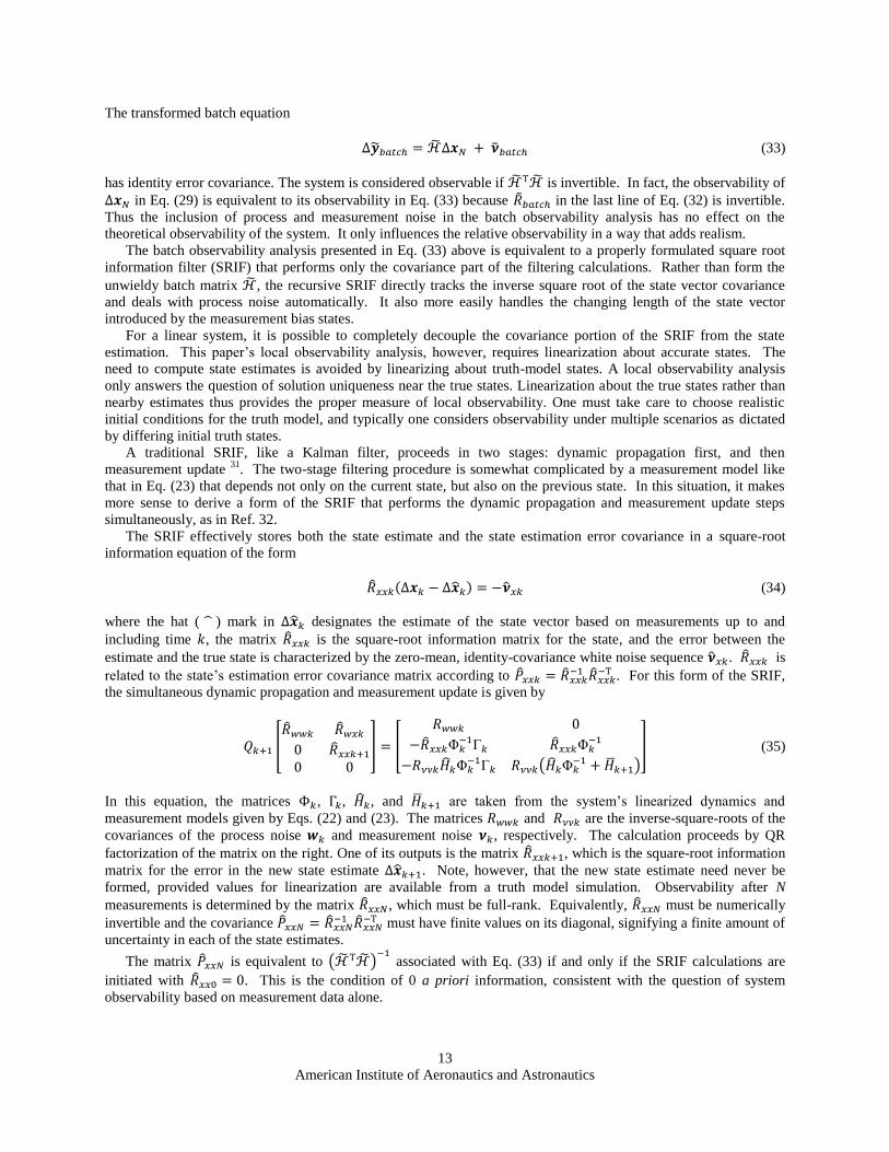
The transformed batch equation

(33)

has identity error covariance. The system is considered observable if is invertible. In fact, the observability of

in Eq. (29) is equivalent to its observability in Eq. (33) because in the last line of Eq. (32) is invertible.

Thus the inclusion of process and measurement noise in the batch observability analysis has no effect on the

theoretical observability of the system. It only influences the relative observability in a way that adds realism.

The batch observability analysis presented in Eq. (33) above is equivalent to a properly formulated square root

information filter (SRIF) that performs only the covariance part of the filtering calculations. Rather than form the

unwieldy batch matrix , the recursive SRIF directly tracks the inverse square root of the state vector covariance

and deals with process noise automatically. It also more easily handles the changing length of the state vector

introduced by the measurement bias states.

For a linear system, it is possible to completely decouple the covariance portion of the SRIF from the state

estimation. This paper’s local observability analysis, however, requires linearization about accurate states. The

need to compute state estimates is avoided by linearizing about truth-model states. A local observability analysis

only answers the question of solution uniqueness near the true states. Linearization about the true states rather than

nearby estimates thus provides the proper measure of local observability. One must take care to choose realistic

initial conditions for the truth model, and typically one considers observability under multiple scenarios as dictated

by differing initial truth states.

A traditional SRIF, like a Kalman filter, proceeds in two stages: dynamic propagation first, and then

measurement update 31

. The two-stage filtering procedure is somewhat complicated by a measurement model like

that in Eq. (23) that depends not only on the current state, but also on the previous state. In this situation, it makes

more sense to derive a form of the SRIF that performs the dynamic propagation and measurement update steps

simultaneously, as in Ref. 32.

The SRIF effectively stores both the state estimate and the state estimation error covariance in a square-root

information equation of the form

(34)

where the hat ( ) mark in designates the estimate of the state vector based on measurements up to and

including time , the matrix is the square-root information matrix for the state, and the error between the

estimate and the true state is characterized by the zero-mean, identity-covariance white noise sequence . is

related to the state’s estimation error covariance matrix according to

. For this form of the SRIF,

the simultaneous dynamic propagation and measurement update is given by

(35)

In this equation, the matrices , , , and are taken from the system’s linearized dynamics and

measurement models given by Eqs. (22) and (23). The matrices and are the inverse-square-roots of the

covariances of the process noise and measurement noise , respectively. The calculation proceeds by QR

factorization of the matrix on the right. One of its outputs is the matrix , which is the square-root information

matrix for the error in the new state estimate . Note, however, that the new state estimate need never be

formed, provided values for linearization are available from a truth model simulation. Observability after N

measurements is determined by the matrix , which must be full-rank. Equivalently, must be numerically

invertible and the covariance

must have finite values on its diagonal, signifying a finite amount of

uncertainty in each of the state estimates.

The matrix is equivalent to

associated with Eq. (33) if and only if the SRIF calculations are

initiated with . This is the condition of 0 a priori information, consistent with the question of system

observability based on measurement data alone.

14


If the system is unobservable, it may be reasonable to relax slightly the assumption that . Typically, one

has some a priori information, such as a bound on the physically realistic range of inverse ballistic coefficients.

Such information can be incorporated into and may make the system practically observable.

V. Results

The observability analysis was performed in several stages. First, a truth model was used to generate several

representative system state histories. Next, the dynamics and measurement models of Eqs. (6) and (21) were

linearized around these “truth” states as in Eqs. (22)-(23). The SRIF covariance calculations yielded , the

square-root information matrix for the state after measurements. Finally, and the estimation error covariance

were examined to determine observability.

A. Truth model cases

The truth model for a representative case used for this paper’s analysis includes 66 satellites in 6 nearly polar

orbital planes. Each satellite has a near-circular orbit, and the mean orbit altitude for all satellites is 790 km. The

satellites are modeled as each having approximately the same truth-cross-sectional area and mass, such that the

mean ratios are

m

2/kg and

m

2/kg, and the inverse ballistic coefficient

and

solar radiation pressure coefficient are slowly-varying random walks that are essentially constants over the batch

lengths considered in this paper. The satellite clocks are assumed to have noise characterized by

(36)

These process noise intensities correspond to an equivalent root Allan variance of at a delay of 139 sec,

typical of a good oven-controlled crystal oscillator (OCXO) 26

under benign conditions.

The satellites are tracked by 12 ground

reference stations. Each ground station also

receives GPS signals that are used to

discipline the ground station clocks. The

ground stations are located as shown in the

map in Figure 2.

Within each orbital plane, adjacent

satellites are connected by crosslink

measurements, and every ground station has

phase and pseudorange downlink

measurements from all satellites above an

elevation of . For simplicity, all the

crosslink and downlink measurements have

sampling rates of 5 seconds. The crosslink

accumulated delta range measurements are

modeled as having measurement error

standard deviations of 3.4 cm. On the accumulated delta range downlink measurements, the measurement error

standard deviations are 0.3 mm. In contrast, the unbiased but imprecise pseudoranges have measurement error

standard deviations of 30 m. Note: These accuracies assume averaging of less accurate, higher frequency data over

5-second intervals.

The “truth” splined atmospheric density distribution is initialized by fitting to the outputs of the NRLMSISE-00

model evaluated for January 21 at 08:03:20 UTC, with = 150, the 81-day average = 150, and = 4. The

spline has 6 longitude nodes and 5 latitude nodes, including the poles. Markov time constants of = 3 hours were

selected based on the maximum available time resolution of the geomagnetic and solar indices, which in turn limits

Figure 2. Map of ground reference stations

15


the resolution of standard models that use these indices as inputs. The intensity of the driving process noise is

known to be related to the steady-state variance of according to

(37)

where , the steady-state variance of , is chosen to yield an equivalent density steady-state standard deviation of

approximately 70%. For simplicity, the elements and are assumed to be uncorrelated for .

The truth model simulation was performed for a batch length of 12 hours. The samples all had equal lengths of 5

seconds.

Other truth model cases for which observability has been analyzed are similar to this representative case in many

respects. They attempt to isolate the effects on observability of certain types of changes. For instance, one doubles

the batch length to 24 hours. Another alternate case uses the lower constellation altitude of 500 km.

Of course one could think of many other interesting cases. These might include changes of atmospheric Markov

time constants or process noise intensities to explore performance under conditions of high solar activity,

changes of measurement precision, changes in the set of ground reference stations, or changes to the constellation

configuration. For the sake of brevity, a total of only three cases are considered here.

B. Representative observability results

The observability analysis results

presented here are for the representative

case described in the previous

subsection. In this instance, the square-

root information matrix was full-

rank, as demonstrated by the success of

the numerical inversion

. The

system was still deemed unobservable,

however, because the diagonal elements

of corresponding to the

atmospheric parameter vector all

had very large values, orders of

magnitude above the parameter values

themselves. Closer examination

revealed that these standard deviations

were decreasing and had not yet

reached a steady state at the end of the

12 hour batch, as shown in Figure 3.

For this representative case, the square-

root information matrix contained

no a priori information about the

atmospheric density parameters or the

inverse ballistic coefficients, so effectively the initial covariance was infinite. The finite standard deviations shown

in Figure 3 mean that the crosslink and downlink measurements did improve the estimates of those parameters. The

measurements were not sufficient, however, to achieve trustworthy estimates within a reasonable amount of time,

and so this particular case can be considered practically unobservable.

Despite the large remaining uncertainties associated with , the satellite orbit accuracies were reasonable for

this representative case, as were those of the inverse ballistic coefficient, solar radiation pressure coefficient, and

other satellite-specific states. Figure 4 shows the estimation error standard deviations for one satellite in the

altitude/along-track/cross-track directions, and Figure 5 likewise gives the estimation error standard deviations for

the same satellite’s drag and solar pressure coefficients. The high level of orbital position accuracy in Figure 4 is

somewhat surprising, given the poor accuracy of the atmospheric parameters. These results suggest that this is a

data-rich orbit estimation problem, in which the final accuracy is insensitive to significant levels of dynamic model

error. It is conjectured that the crosslinks are the key to this data richness.

Figure 3. Estimation error standard deviations for the elements of ,

representative case

16


In an attempt to overcome the original unobservability of

the system, a priori knowledge was incorporated by setting

some of the elements in to non-zero values. To begin

with, the elements corresponding to inverse ballistic

coefficients were adjusted to reflect a physically realistic

level of initial uncertainty about these values for well-

characterized satellites. Most notably, this had the effect of

reducing the uncertainty about inverse ballistic coefficients

throughout the entire 12-hour batch, as illustrated for one

satellite in Figure 6. The diagonal elements of

corresponding to the satellite orbit states and the atmospheric

parameters initially decreased more quickly, but after three or

four hours the standard deviations returned to those of the first

representative case. This transient effect is shown in Figure 7

and Figure 8. Such behavior suggests that errors in the

estimates of inverse ballistic coefficients are not a major

contributor to errors in estimates, at least in the long term.

Figure 8. Comparison of atmospheric parameters

estimation error standard deviations, showing

transient behavior

Figure 7. Comparison of position estimation error

standard deviations for one satellite, showing

transient behavior

Figure 5. Estimation error standard deviations for one

satellite's inverse ballistic coefficient and solar

radiation pressure coefficient

Figure 4. Estimation error standard deviations for one

satellite’s position (in the altitude/along-track/cross-

track directions)

Figure 6. Comparison of inverse ballistic

coefficient estimation error standard deviations,

with and without a priori knowledge included

17


Of course, changes in the Markov time constants of the atmospheric states could affect this lack of coupling,

especially if the time constants increased dramatically. Such an increase would yield a random-walk-like model.

Further observability improvements were attempted by incorporating some reasonable a priori information about

the atmospheric density parameter vector , consistent with the amount of knowledge available from existing

atmospheric density models. This was accomplished by setting the corresponding diagonal elements of to the

inverse of the chosen Markov process standard deviations. At steady state with no incoming measurements, this is

the amount of uncertainty that would be expected in with the given dynamic model. Consequently, any

reduction in the diagonal elements of indicates that the atmospheric parameters are observable and the

measurements are reducing the uncertainty associated with the density estimates.

The uncertainty in the elements of does indeed decrease from its initial level over the batch interval, as shown

in Figure 9. Several things can be observed in this figure. First, the elements of the parameter vector span

several orders of magnitude and are not all measured in the same units, so they cannot all be clearly visualized on

one plot. The horizontal lines in the lower part of the Figure 9 are actually decreasing standard deviations

corresponding to lower-magnitude elements, but the scale obscures the reduction in uncertainty. Next, while some

standard deviations on this plot decrease rapidly, others are only mildly observable and the reduction is slight. One

significant difference between Figure 9 and Figure 3 from the baseline representative case, other than the plot scale,

is the way in which many of the standard

deviations in this figure appear to reach a

steady-state value before the end of the

interval. These steady-state standard

deviations suggest that additional

measurements beyond this batch will not

greatly improve the density estimates. A

final interesting feature of this plot is the

high-frequency oscillation evident in many of

the standard deviation elements at

equilibrium. Its period of about 8-10 minutes

suggests that it may be related to the time

interval between flybys of two consecutive

satellites at a given location; the passage of a

satellite could temporarily improve local

density information.

Interpreting the results of a plot like

Figure 9 is clearly challenging, particularly

with so many different units and orders of

magnitude represented in . After all, the

real quantity of interest is density itself, and

not some set of spline parameters with

limited physical meaning. To this end, a

method is desired to calculate the standard deviation of the density estimation error for an arbitrary position in the

constellation. Such a method is readily available by using the partial derivative

to transform the covariance of

the estimates into standard deviations of density . The transformation takes the form

(38)

where is the density estimation error standard deviation for the location at which the derivative

was

evaluated, and is the block of the covariance matrix corresponding to the elements of . Equation (38)

has been applied to a number of random globally distributed points to determine the overall effect of the

measurements on the density estimates when a priori information about has been employed. Averaged over

1000 points in the constellation region, the normalized standard deviation at the beginning of the batch interval

was 0.71. At the end of 12 hours, the average was 0.44, indicating a significant uncertainty reduction. For a

better visualization of this overall drop in uncertainty, see Figure 10 and Figure 11, which have been plotted on the

same scale for easy comparison.

Figure 9. Estimation error standard deviations for elements of ,

with a priori density information

18


In these figures, normalized density standard deviation is plotted versus latitude and longitude. The regular, bumpy

pattern is closely aligned with the grid of points underlying the spline structure of the atmospheric density

representation. It is at least in part an artifact of non-optimal relative scaling of , the chosen steady-state Markov

process standard deviations of the individual elements of . It is difficult to scale the initial uncertainties of

bicubic spline parameters in a way that would produce a perfectly flat plot in Figure 10. The figures nevertheless

clearly show an overall reduction in uncertainty level over the course of the 12-hour batch interval.

C. Other scenarios

When the batch length was doubled relative to the representative case, it had only minor effects on the results.

In general, the main difference was that some of the estimation error standard deviations that had not completely

reached a steady state in 12 hours were able to do so in 24 hours. For instance, Figure 12 shows the evolution of the

position estimation error standard deviations for one satellite over the 24-hour batch. The end of the 12-hour batch,

marked with the dashed line, came just as the standard deviations were starting to level out more completely. The

leveling out of cross-track standard deviation at 12 hours may be due to the fact that 12 hours is the required time for

each orbital plane to see every ground station. Likewise, Figure 13 is a zoomed plot showing just some of the

atmospheric parameter standard deviations.

Figure 13. Atmospheric parameter estimation error

standard deviations over 24-hour batch

Figure 12. Position estimation error standard

deviations for one satellite over 24-hour batch

Figure 11. Normalized standard deviation of density

estimate after 12-hour batch interval

Figure 10. Normalized standard deviation of density

estimate before measurements

19


At the 12-hour mark, many of the uncertainties are still decreasing, but by about 20 hours they seem to reach

equilibrium. Despite the extra time for the estimates to approach a steady state, the density estimate itself does not

improve measurably with the doubled batch length.

For the alternate case of a lower constellation altitude described in Subsection A above, the system was expected

to be more observable. This is because the combination of greater density and greater satellite velocities results in a

more significant influence on satellite orbits. As Figure 14 illustrates, this was indeed the case. The standard

deviations of the parameter state estimates decreased more quickly and reached lower values relative to the higher-

altitude case. Oscillations at both the orbital frequency and the satellite flyby frequency are clearly visible in this

data set. Figure 15 shows the mean normalized density standard deviations at 3-hour intervals over the 12-

hour batch. After only 3 hours, they reached a steady state of about 0.25, as opposed to only 0.44 for the case of

higher constellation altitude.

Although the density accuracy improved at 500 km altitude,

Figure 16 shows that the satellite position accuracies got slightly

worse. Most likely this is because the greater influence of the

higher density made the orbit accuracy more susceptible to model

errors and atmospheric density uncertainty. Also, each satellite at

this lower altitude is tracked by the 12 ground stations less

frequently, and the duration of a given pass is shorter, leading to

fewer total measurements.

D. Computational load

Although these observability calculations have been run

offline, they give an indication of whether a corresponding

recursive filter could run in real-time. This is an important

question given the complexity of the system. The number of

satellites in the constellation and the chosen resolution of the

atmospheric density spline dictate that the state vector contains

approximately 1170 elements. At any given time the number of state vector elements depends on the number of

measurement biases. Numerical integration of the satellite states and associated linearized model matrices is costly.

Also of concern are the QR factorization operations that implement the covariance propagation and update steps and

the necessary inversions of very large matrices. The dynamic propagation operations scale linearly as states are

added, but QR factorization scales as the cube of the number of states. Calculations were performed in MATLAB on

a computer with a 2.5 GHz Intel Q9300 quad core processor and 4 GB of RAM, operating with 64-bit Windows

Vista Business. For a typical observability analysis procedure, the dynamic propagation calculations ran for about

1.1 seconds per 5-second sample. The SRIF covariance computations took about 3.6 seconds per 5-second sample.

Figure 15. Mean normalized density standard

deviations during 12-hour batch for 500 km-altitude

case

Figure 14. Comparison of estimation error

standard deviations for the elements of at 790

km and 500 km altitudes

Figure 16. Comparison of one satellite's

position accuracies at 790 km and 500 km

altitudes

20


In combination and with some additional overhead, the analysis ran approximately in real time. Note that the

dynamic propagation calculations can be run in parallel for different satellites.

E. Possible future studies

This paper’s results suggest several related avenues for future research. One would be to use real data from a

satellite constellation in a filter form of this paper’s algorithm. Another useful effort would re-cast the treatment of

implicitly defined transmission and reception times into the framework of Ref. 29. Its framework deals with

interpolation and process noise in a more rigorous manner.

VI. Summary and Conclusions

A new atmospheric density calibration scheme has been developed that focuses on estimating a density

distribution based on data from a satellite constellation. This strategy simultaneously improves the constellation

orbit estimates. It leverages a rich data set of radiocommunication signals and does not require any dedicated

sensors for satellite motion tracking. As part of the formulation of the estimation problem, this paper also introduces

a new spline-based atmospheric density parameterization. Compared with other density representation methods, this

parameterization fits more naturally into the estimation context without reducing the resolution of the density

distribution.

A linearized observability analysis has been performed for the system that consists of the constellation, the radio

signals, and the density distribution. This analysis aims to discover not only whether the system is theoretically

observable, but also what types of assumptions or a priori knowledge might be expected to improve observability.

The results show that some a priori knowledge about density is necessary to reduce uncertainty in atmospheric

density estimates. Furthermore, knowledge about the satellite inverse ballistic coefficients is of limited use, because

the difference in time constants tends to decouple the inverse ballistic coefficients and the density parameters if the

batch is long enough. Given a reasonable initial guess of the atmospheric density spline parameters, however, the

measurements do contribute to greater density estimation accuracy. Another interesting result is that the rich data

set provided by the crosslink and downlink measurements makes satellite orbit accuracies relatively insensitive to

some dynamic model errors. A test case with a lower constellation altitude demonstrates the effects of higher

density: Due to its greater influence on the satellite orbits, density becomes more observable while decreasing the

orbital position accuracies. The overall results suggest that further study of the proposed scheme for simultaneous

atmospheric density calibration and constellation orbit determination would be worthwhile.

Appendix

Section II of this paper gives a conceptual overview of the spline-based atmospheric density parameterization,

but it does not provide all of the details helpful for implementation. Those details are contained in this appendix. In

particular, emphasis is placed on the derivation of necessary equations and on some practical implementation

challenges.

A. Spline equations

As explained in Section II, the basic form of the splined parameterization is given by

(A1)

where the quantities and are parameterized by two-dimension cubic spline functions. In what follows,

equations are given in terms of the spline, but are equally applicable to any spline-parameterized quantity. The

spline functions essentially work by interpolation. The parameter vector stores and partial and cross-partial

derivatives of that apply at a rectangular grid of latitude and longitude points. Values of at any non-grid point

are obtained by interpolating between the stored values.

21


Two-dimensional bicubic spline interpolation assumes that the desired

values can be written as cubic functions of their two-dimensional position.

Given a particular latitude and longitude , one can identify a

normalized “grid cell” within which the point of interest lies, as in Figure

A1. In this figure, the normalized coordinates and vary from 0 to 1.

is given by a weighted sum of powers of these coordinates up

to the cubic terms:

(A2)

The weights are functions of the values of and its derivatives at the four corners of the grid cell. Suppose

that the corner values are given by the vector

(A3)

Then the 16 weights can be found as a vector using the equation

(A4)

Figure A1. Basic spline function grid

notation

Caption here (Figure A1)

22


where the matrix is

(A5)

and the vector contains the stacked scalar weights :

(A6)

If desired, spatial derivatives of are easily obtained from Eq. (A2):

(A7a)

(A7b)

(A7c)

Equations (A2) and (A7) can also be written in a matrix form, which may be convenient for certain computations.

To do this, create a vector of the coordinates raised to powers from 0 to 3:

(A8)

Then Eq. (A2), along with the weight vector of Eq. (A4), becomes

(A9)

One forms the equivalent expressions for the partial derivatives by taking derivatives of the vector with respect

to and . Derivatives with respect to true latitude and longitude (rather than normalized latitude and longitude)

require a conversion from normalized grid cell units to radians.

B. Constraints

Although the spline interpolation described above works well to describe density over a rectangular region,

problems arise when one applies it to a sphere or ellipsoid. As described in Section II, certain constraints are

required to maintain consistency and ensure a smooth variation of density over the entire globe.

First, one must consider that longitudes of and correspond to the same physical location.

Consequently, should store only one set of values for and its derivatives along this meridian, rather than two

sets. Any computer implementation must index into the vector in such a way that it retrieves the same values for

either nominal longitude.

Second, a more complicated set of constraints arises at the two poles. Only one value of is stored in for

each of the poles, so that near the North pole, for instance, points and of Fig. A1 have the same value. This

23


means that a single element of is mapped to two elements of the vector , which is in turn used to define the

weights for the cubic function.

Constraining the derivatives to ensure smooth variation of density over the polar regions requires careful

thought. While all longitudes may become equivalent at these singularities, the derivatives with respect to latitude

will depend on the longitude from which the pole is approached. The nature of the necessary constraints is not

obvious, but the following analysis provides some clarity.

First, assume that is varies smoothly over the ellipsoidal surface parameterized by and . It can be

equivalently written as a function of Cartesian coordinates , where , , and are related to and

by

(A10)

The scalars and determine the size and shape of the ellipsoid. Cartesian coordinates have the advantage of

having no singularities at the poles.

As is fully differentiable, one can take derivatives with respect to , , and and then use the chain rule to

compute partial derivatives with respect to and . Then one evaluates those derivatives at . The

longitude derivatives are

(A11)

After taking partial derivatives of the Cartesian variables according to (A10) and substituting those expressions into

(A11), one obtains

(A12)

At either pole, , so

(A13)

Next, follow the same procedure by taking latitude derivatives. First,

(A14)

Substituting the derivatives of Eq. (A10), (A14) becomes

(A15)

When (A15) is evaluated at each pole, the result is

(A16a)

(A16b)

24


Finally, the same process is applied to calculate the cross-partial derivatives with respect to latitude and

longitude. After some algebra, and recalling that , all the higher order derivatives with respect to the

Cartesian variables vanish. The remaining non-zero expressions are

(A17a)

(A17b)

It should be noted that Eqs. (A17) are very similar in form to Eqs. (A16). This similarity can be stated more

explicitly by defining some new variables:

(A18a)

(A18b)

(A18c)

(A18d)

After substituting Eqs. (A18) into Eqs. (A16) and (A17), one obtains

(A19a)

(A19b)

(A19c)

(A19d)

The key result, as expressed in Eqs. (A19), is that all the partial derivatives at the poles are completely specified

by just two parameters per pole. For a given longitude, the standard spline-form derivatives can be determined from

these two parameters, which are thus the only quantities stored in the vector to represent all the partial

derivatives at each pole. This result makes sense if one considers what it means for to be differentiable at the

poles: in a sufficiently small region surrounding each pole, one can think of as locally looking like a flat plane,

which is completely described by its tilt direction and angle.

C. Parameter transformation

Although to this point the splined atmosphere representation has been described in terms of the quantities and

, it is really only correct to say that the two sets of cubic spline values encode the information about these

quantities. In actual implementation, the vector contains values of and and the derivatives of

those quantities rather than and directly.

There are several reasons for these nonlinear transformations. First, physical density can never be negative, but

standard estimation procedures provide no easy way to prevent estimates from becoming negative if inaccurate

measurements so indicate. By calculating density as , this situation is averted. Second, the logarithmic

transformation makes the two spline functions add together linearly, which aids computational ease significantly.

To demonstrate this, take the natural logarithm of both sides of Eq. (A1):

(A20)

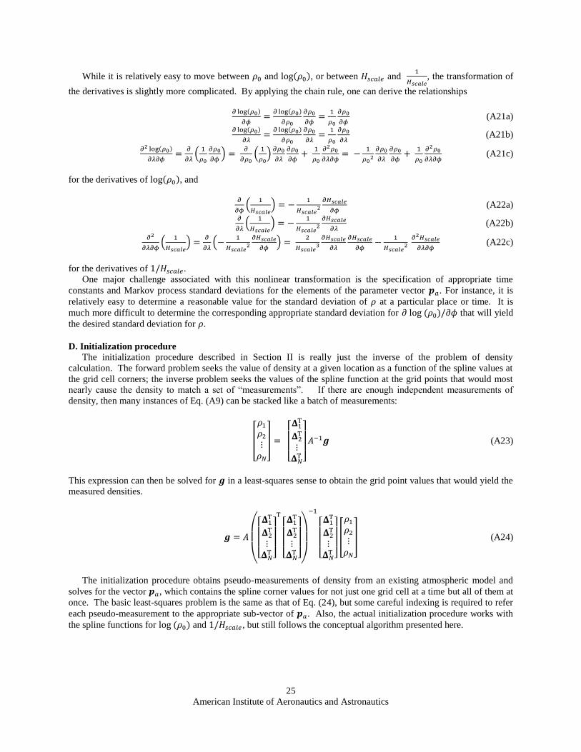
25


While it is relatively easy to move between and , or between and

, the transformation of

the derivatives is slightly more complicated. By applying the chain rule, one can derive the relationships

(A21a)

(A21b)

(A21c)

for the derivatives of , and

(A22a)

(A22b)

(A22c)

for the derivatives of .

One major challenge associated with this nonlinear transformation is the specification of appropriate time

constants and Markov process standard deviations for the elements of the parameter vector . For instance, it is

relatively easy to determine a reasonable value for the standard deviation of at a particular place or time. It is

much more difficult to determine the corresponding appropriate standard deviation for that will yield

the desired standard deviation for .

D. Initialization procedure

The initialization procedure described in Section II is really just the inverse of the problem of density

calculation. The forward problem seeks the value of density at a given location as a function of the spline values at

the grid cell corners; the inverse problem seeks the values of the spline function at the grid points that would most

nearly cause the density to match a set of “measurements”. If there are enough independent measurements of

density, then many instances of Eq. (A9) can be stacked like a batch of measurements:

(A23)

This expression can then be solved for in a least-squares sense to obtain the grid point values that would yield the

measured densities.

(A24)

The initialization procedure obtains pseudo-measurements of density from an existing atmospheric model and

solves for the vector , which contains the spline corner values for not just one grid cell at a time but all of them at

once. The basic least-squares problem is the same as that of Eq. (24), but some careful indexing is required to refer

each pseudo-measurement to the appropriate sub-vector of . Also, the actual initialization procedure works with

the spline functions for and , but still follows the conceptual algorithm presented here.

26


E. Partial derivatives

As discussed in Section II, the estimation problem requires the partial derivatives

and

. Equation (A7)

readily provides

,

,

, and

. Differentiation of a modified form of Eq. (A23) gives

and

. The required derivatives can be computed from the available ones by repeated application of the chain

rule. For

, this is a relatively simple procedure involving some minor algebraic manipulation. The final result is

(A25)

In order to compute

, the partial derivative of density with respect to inertial position, one first finds

derivatives of density with respect to latitude, longitude, and altitude. Starting with Eq. (A1) and after some

straightforward differentiation and algebra, these expressions are

log

(A26a)

(A26b)

(A26c)

Note that the constellation nominal altitude is a function of latitude because it depends on the local radius of the

WGS-84 ellipsoid. Its derivative

can be obtained by differentiating the ellipsoid equations.

The next step involves the derivatives that transform from latitude, longitude, and altitude to an Earth-fixed

position, and then from Earth-fixed coordinates to inertial coordinates. The resulting expression is

(A27)

where

,

, and

are assumed to be available from the algorithm that converts latitude, longitude, and

altitude to a Cartesian position vector, and is the time-varying rotation matrix that transforms between the

Earth-fixed and inertial coordinate systems.

References 1 Puderbaugh, A.L., Dixon, G.L., Jr., Shroyer, L.E., Boyce, W.H. III, and Shepperd, R.W., “A Global and Local History of

Drag Effects at Iridium Mission Altitude,” Proc. of AIAA/AAS Astrodynamics Specialist Conference and Exhibit, 5-8 August

2002, Monterey, CA, AIAA 2002-4733 (2002). 2 Jacchia, L.G., “Density Variations in the Heterosphere,” Smithsonian Astrophysical Observatory Special Report #184,

Cambridge, MA, 1965. 3 Jacchia, L.G., “New Static Models of the Thermosphere and Exosphere with Empirical Temperature Profiles,” Smithsonian

Astrophysical Observatory Special Report #313, Cambridge, MA, 1970. 4 Jacchia, L.G., “Thermospheric Temperature, Density, and Composition: New Models,” Smithsonian Astrophysical

Observatory Special Report #375, Cambridge, MA, 1977. 5 Roberts, C.E., “An Analytical Model for Upper Atmosphere Densities Based Upon Jacchia’s 1970 Models,” Celestial

Mechanics, Vol. 4, December 1971, pp. 368-377. 6 Hedin, A.E., “The Atmospheric Model in the Region 90 to 2000 km,” Adv. in Space Research, Vol. 8, No. 5, 1988, pp. 9-

25. 7 Hedin, A.E., “Extension of the MSIS Thermosphere Model into the Middle and Lower Atmosphere,” J. of Geophysical

Research, Vol. 96, No. A2, February 1991, pp. 1159-1172. 8 Picone, J.M., Hedin, A.E., Drob, D.P., and Aikin, A.C., “NRLMSISE-00 Empirical Model of the Atmosphere: Statistical

Comparisons and Scientific Issues,” J. of Geophysical Research, Vol. 107, No. A12, 2002, pp. 1468-1483. 9 Marcos, F.A., Wise, J.O., Kendra, M.J., and Grossbard, N., “Advances in Satellite Drag Modeling,” Proc. of 42nd AIAA

Aerospace Sciences Meeting and Exhibit, 5-8 January 2004, Reno, NV, AIAA 2004-1254 (2004).

27


10 Lean, J., Picone, J.M., Knowles, S., Hedin, A., and Moore, G., “Validating NRLMSIS Using Atmospheric Densities

Derived from Spacecraft Drag: Starshine Example,” Proc. of AIAA/AAS Astrodynamics Specialist Conference and Exhibit, 5-8

August 2002, Monterey, CA, AIAA 2002-4736 (2002). 11 Pardini, C. and Anselmo, L., “Comparison and Accuracy Assessment of Semi-empirical Atmosphere Models through the

Orbital Decay of Spherical Satellites,” J. of the Astronautical Sciences, Vol. 49, No. 2, 2001, pp. 255-268. 12 Marcos, F.A., Kendra, M.J., Griffin, J.M., Bass, J.N., Larson, D.R., and Liu, J.J., “Precision Low Earth Orbit

Determination Using Atmospheric Density Calibration,” J. of the Astronautical Sciences, Vol. 46, No. 4, Oct.-Dec. 1998, pp.

395-409. 13 Marcos, F.A., Kendra, M.J., and Bass, J.N., “Recent Advances in Satellite Drag Modeling,” Proc. of 37th AIAA Aerospace

Sciences Meeting and Exhibit, 11-14 January 1999, Reno, NV, AIAA 99-0631 (1999). 14 Bowman, B.R., Tobiska, W.K., Marcos, F.A., Huang, C.Y., Lin, C.S., and Burke, W.J., “A New Empirical Density Model

JB2008 Using New Solar and Geomagnetic Indices,” Proc. of AIAA/AAS Astrodynamics Specialist Conference, 18-21 August

2008, Honolulu, HI, AIAA 2008-6438 (2008). 15 Hedin, A.E., and Carignan, G.R., “Morphology of Thermospheric Composition Variations in the Quiet Polar

Thermosphere From Dynamics Explorer Measurements,” J. of Geophysical Research, Vol. 90, No. A6, June 1985, pp 5269-

5277. 16 Yunck, T.P., “Coping with the Atmosphere and Ionosphere in Precise Satellite and Ground Positioning,” Geophysical

Monograph Series, Vol. 73, A. Jones (ed.), American Geophysical Union, Washington, D.C., 1993, pp. 1-16. 17 DeBra, D.B., “Drag-Free Spacecraft as Platforms for Space Missions and Fundamental Physics,” Class. Quantum Grav.,

Vol. 14, 1997, pp. 1549-1555. 18 Nazarenko, A.I., Cefola, P.J., and Yurasov, V., “Estimating Atmospheric Density Variations to Improve LEO Orbit

Prediction Accuracy,” Proc. of the AAS/AIAA Spaceflight Mechanics Meeting, 1998, pp 1235-1264. 19 Yurasov, V.S., Nazarenko, A.I., Alfriend, K.T., and Cefola, P.J., “Direct Density Correction Method: Review of Results,”

Proc. of 57th Intl. Astronautical Conf., Valencia, Spain, 2-6 October 2006. 20 Picone, J.M., Emmert, J.T., and Lean, J.L., “Thermospheric Densities Derived from Spacecraft Orbits: Accurate

Processing of Two-Line Element Sets,” J. of Geophysical Research, Vol. 110, No. A03301, 2005. 21 Doornbos, E., Klinkrad, H., and Visser, P., “Use of Two-Line Element Data for Thermosphere Neutral Density Model

Calibration,” Adv. in Space Research, Vol. 41, 2008, pp. 1115-1122. 22 Casali, S.J., and Barker, W.N., “Dynamic Calibration Atmosphere (DCA) for the High Accuracy Satellite Drag Model

(HASDM),” Proc. of Astrodynamics Specialist Conference and Exhibit, 5-8 August 2002, Monterey, CA, AIAA 2002-4888

(2002). 23 Storz, M.F., Bowman, B.R., Branson, Major J.I., Casali, S.J., and Tobiska, W.K., “High Accuracy Satellite Drag Model

(HASDM),” Adv. in Space Research, Vol. 36, 2005, pp. 2497-2505. 24 Anderson, R.L., Born, G.H., and Forbes, J.M., “Sensitivity of Orbit Predictions to Density Variability,” J.of Spacecraft and

Rockets, Vol. 46, No. 6, 2009, pp. 1214-1230. 25 Psiaki, M.L., “Autonomous Low-Earth-Orbit Determination from Magnetometer and Sun Sensor Data,” J.of Guidance,

Control, and Dynamics, Vol. 22, No. 2, March-April 1999, pp. 296-304. 26 Brown, R.G. and Hwang, P.Y.C., Introduction to Random Signals and Applied Kalman Filtering with Matlab Exercises

and Solutions, John Wiley & Sons, 3rd Ed., New York (1997), pp. 428-431. 27 Wright, J.R., and Woodburn, J., “Simultaneous Real-Time Estimation of Atmospheric Density and Ballistic Coefficient,”

Paper AAS 04-175, Spaceflight Mechanics 2003-Adv. in the Astronautical Sciences, Vol. 114, pp. 927-950, Proc. of the 13th

AAS/AIAA Space Flight Mechanics Conf., Ponce, Puerto Rico, 9-13 February 2003. 28 Wright, J.R., “Real-Time Estimation of Local Atmospheric Density,” Paper AAS 03-164, Spaceflight Mechanics 2005-

Adv. in the Astronautical Sciences, Vol. 119, pp. 1155-1184, Proc. of the 14th AAS/AIAA Space Flight Mechanics Conf., Maui,

HI, 8-12 February 2004. 29 Mohiuddin. S., and Psiaki, M.L., “Continuous-Time Kalman Filtering with Implicit Discrete Measurement Times,”

submitted to the Journal of Guidance, Control, & Dynamics, in review. 30 Mitch, R.H., and Psiaki, M.L., “Local Ionosphere Model Estimation from Dual-Frequency GNSS TEC Data,” to be

presented at ION GNSS 2010, Portland, OR, 21-24 September 2010. 31 Bierman, G.J., Factorization Methods for Discrete Sequential Estimation, Academic Press, New York, 115-122 (1977) ,

pp. 69-76. 32 Psiaki, M.L., and Hinks, J.C., “Autonomous Lunar Orbit Determination using Star Occultation Measurements,” Proc. of

AIAA Guidance, Navigation, and Control Conference and Exhibit, 20-23 August 2007, Hilton Head, SC, AIAA 2007-6657

(2007).

simultaneous orbit and atmospheric density estimation for

Documents