simultaneous optimization of transfer prices and good flows against two-step sequential one
TRANSCRIPT

Optimal Management, LLC
Demo calculation for optimization of simplified supply chain in multinational enterprise
The comparison of Two-step optimization
• first optimization of production and logistic (minimizing costs),
• then optimization of taxation (maximizing profit by varying
transfer prices)
One-step simultaneous optimization of transfer prices,
production and logistic parameters
and

2
Presentation’s
agenda
• Demo Supply Chain’s structure…….………...3
• Demo Supply Chain’s data….………………….5
• Variants of calculations...…………………..…14
• Comparison of calculation’s results….….....18
• The specificity of problem…….…….……..…20
• Rendering the service…………….…….…..…21
3
Supply chain’s
structure

4
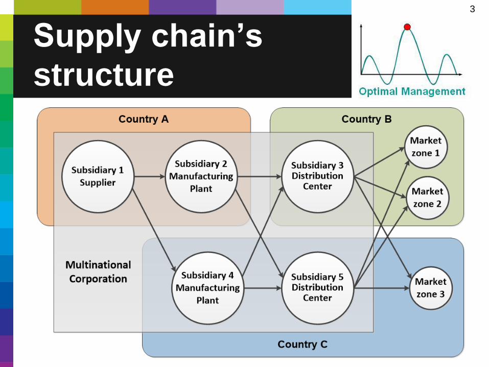
• Subsidiary 1 in Country A produces Raw Material and sells it
to Subsidiary 2 in Country A and Subsidiary 4 in Country C.
• Subsidiary 2 in Country A produces Finished Product and
sells it to Subsidiary 3 in Country B and Subsidiary 5 in
Country C.
• Subsidiary 4 in Country C produces Finished Product and
sells it to Subsidiary 3 in Country B and Subsidiary 5 in
Country C.
• Subsidiary 3 in Country B sells Finished Product to Market
zone 1, Market zone 2 and Market zone 3.
• Subsidiary 5 in Country C sells Finished Product to Market
zone 1, Market zone 2 and Market zone 3.
Supply chain’s
structure
5
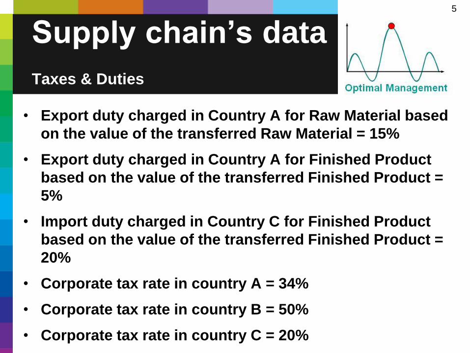
• Export duty charged in Country A for Raw Material based
on the value of the transferred Raw Material = 15%
• Export duty charged in Country A for Finished Product
based on the value of the transferred Finished Product =
5%
• Import duty charged in Country C for Finished Product
based on the value of the transferred Finished Product =
20%
• Corporate tax rate in country A = 34%
• Corporate tax rate in country B = 50%
• Corporate tax rate in country C = 20%
Supply chain’s data
Taxes & Duties
6
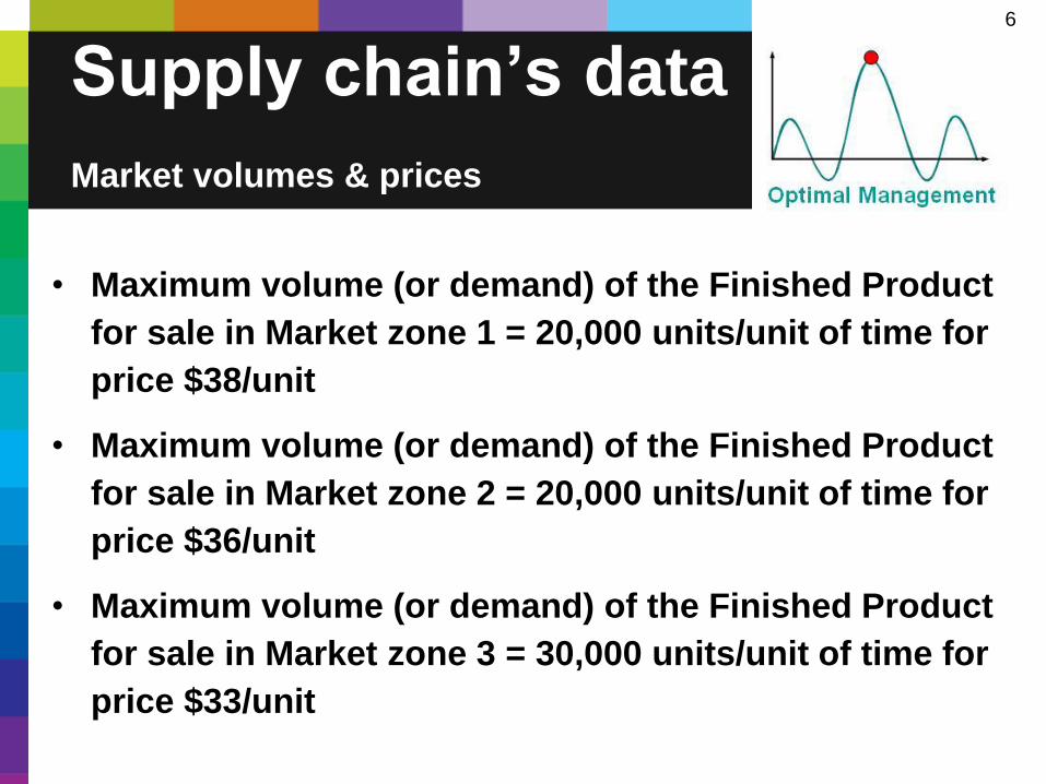
• Maximum volume (or demand) of the Finished Product
for sale in Market zone 1 = 20,000 units/unit of time for
price $38/unit
• Maximum volume (or demand) of the Finished Product
for sale in Market zone 2 = 20,000 units/unit of time for
price $36/unit
• Maximum volume (or demand) of the Finished Product
for sale in Market zone 3 = 30,000 units/unit of time for
price $33/unit
Supply chain’s data
Market volumes & prices

7
• Lower and upper bounds of the transfer prices on Raw
Material between countries A and C = $5 - $6/unit
• Lower and upper bounds of the transfer prices on
Finished Product between countries A and B = $26 - $27
/unit
• Lower and upper bounds of the transfer prices on
Finished Product between countries A and C = $26 - $27
/unit
• Lower and upper bounds of the transfer prices on
Finished Product between countries C and B = $26 - $27
/unit
Supply chain’s data
Intervals of transfer prices

8
• Capacity of Subsidiary 1 = 180,000 units of Raw Material/
unit of time
• Production capacity of Subsidiary 2 = 40,000 units of
Finished Products/unit of time
• Production capacity of Subsidiary 4 = 40,000 units of
Finished Products/unit of time
• Distribution capacity of Subsidiary 3 = 50,000 units of
Finished Products/unit of time
• Distribution capacity of Subsidiary 5 = 50,000 units of
Finished Products/unit of time
Supply chain’s data
Production capacity

9
• Variable costs for producing the Raw Material in
Subsidiary 1 = $2/unit
• Variable costs for producing the Finished Product in
Subsidiary 2 = $7/unit
• Variable costs for producing the Finished Product in
Subsidiary 4 = $5/unit
• Variable costs for distributing the Finished Product in
Subsidiary 3 = $1/unit
• Variable costs for distributing the Finished Product in
Subsidiary 5 = $1/unit
Supply chain’s data
Variable costs

10
• Fixed costs at Subsidiary 1 in Country A = $200,000 /
unit of time
• Fixed costs at Subsidiary 2 in Country A = $120,000 /
unit of time
• Fixed costs at Subsidiary 3 in Country B = $40,000 /
unit of time
• Fixed costs at Subsidiary 4 in Country C = $100,000 /
unit of time
• Fixed costs at Subsidiary 5 in Country C = $20,000 /
unit of time
Supply chain’s data
Fixed costs (other expenses)

11
• Transportation cost for unit of Raw material on Route
Subsidiary1 Subsidiary2 = $2 / unit
• Transportation cost for unit of Raw material on Route
Subsidiary1 Subsidiary4 = $4 / unit
• Transportation cost for unit of Finished Product on
Route Subsidiary 2 Subsidiary 3 = $2 / unit
• Transportation cost for unit of Finished Product on
Route Subsidiary 2 Subsidiary 5 = $5 / unit
• Transportation cost for unit of Finished Product on
Route Subsidiary 4 Subsidiary 3 = $5 / unit
• Transportation cost for unit of Finished Product on
Route Subsidiary 4 Subsidiary 5 = $2 / unit
Supply chain’s data
Transportation costs (1/2)

12
• Transportation cost for unit of Finished Product on
Route Subsidiary 3 Market zone 1 = $8 / unit
• Transportation cost for unit of Finished Product on
Route Subsidiary 3 Market zone 2 = $3 / unit
• Transportation cost for unit of Finished Product on
Route Subsidiary 3 Market zone 3 = $5 / unit
• Transportation cost for unit of Finished Product on
Route Subsidiary 5 Market zone 1 = $10 / unit
• Transportation cost for unit of Finished Product on
Route Subsidiary 5 Market zone 2 = $2 / unit
• Transportation cost for unit of Finished Product on
Route Subsidiary 5 Market zone 3 = $2 / unit
Supply chain’s data
Transportation costs (2/2)

13
• Resource consumption units of Subsidiary 2 = 2.5 units
of Raw Material/unit of Finished Product
• Resource consumption units of Subsidiary 4 = 2.0 units
of Raw Material/unit of Finished Product
Supply chain’s data
Resource consumption

14
Calculation
Without optimization (empirical approach)
Detail Subsidiary 1 Subsidiary 2 Subsidiary 3 Subsidiary 4 Subsidiary 5 MNC
Sales 500 000,00 1 040 000,00 760 000,00 780 000,00 990 000,00 2 470 000,00
360 000,00 720 000,00
Variable costs 320 000,00 280 000,00 40 000,00 150 000,00 30 000,00 820 000,00
Procurement costs 500 000,00 1 040 000,00 360 000,00 780 000,00
Import duty 0,00
Export duty 54 000,00 52 000,00 106 000,00
Fixed costs 200 000,00 120 000,00 40 000,00 100 000,00 20 000,00 480 000,00
Transportation costs 200 000,00 80 000,00 160 000,00 120 000,00 60 000,00 740 000,00
60 000,00 60 000,00
Net Income Before Tax (NIBT) 86 000,00 8 000,00 140 000,00 50 000,00 40 000,00 324 000,00
Taxes 29 240,00 2 720,00 70 000,00 10 000,00 8 000,00 119 960,00
Net Income After Tax (NIAT) 56 760,00 5 280,00 70 000,00 40 000,00 32 000,00 204 040,00
15
Calculation
After optimization of logistic costs (Step1)
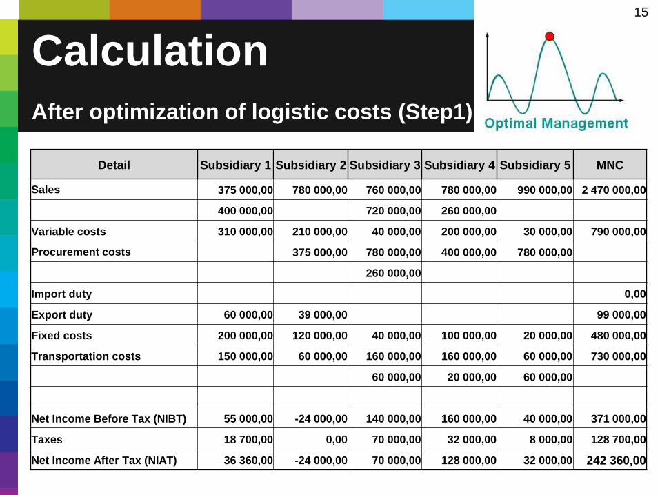
Detail Subsidiary 1 Subsidiary 2 Subsidiary 3 Subsidiary 4 Subsidiary 5 MNC
Sales 375 000,00 780 000,00 760 000,00 780 000,00 990 000,00 2 470 000,00
400 000,00 720 000,00 260 000,00
Variable costs 310 000,00 210 000,00 40 000,00 200 000,00 30 000,00 790 000,00
Procurement costs 375 000,00 780 000,00 400 000,00 780 000,00
260 000,00
Import duty 0,00
Export duty 60 000,00 39 000,00 99 000,00
Fixed costs 200 000,00 120 000,00 40 000,00 100 000,00 20 000,00 480 000,00
Transportation costs 150 000,00 60 000,00 160 000,00 160 000,00 60 000,00 730 000,00
60 000,00 20 000,00 60 000,00
Net Income Before Tax (NIBT) 55 000,00 -24 000,00 140 000,00 160 000,00 40 000,00 371 000,00
Taxes 18 700,00 0,00 70 000,00 32 000,00 8 000,00 128 700,00
Net Income After Tax (NIAT) 36 360,00 -24 000,00 70 000,00 128 000,00 32 000,00 242 360,00

16
Calculation
After optimization of profit by varying of transfer prices (Step2 after Step1)
Detail Subsidiary 1 Subsidiary 2 Subsidiary 3 Subsidiary 4 Subsidiary 5 MNC
Sales 375 000,00 810 000,00 760 000,00 810 000,00 990 000,00 2 470 000,00
400 000,00 720 000,00 270 000,00
Variable costs 310 000,00 210 000,00 40 000,00 200 000,00 30 000,00 790 000,00
Procurement costs 375 000,00 810 000,00 400 000,00 810 000,00
270 000,00
Import duty 0,00
Export duty 60 000,00 40 500,00 100 500,00
Fixed costs 200 000,00 120 000,00 40 000,00 100 000,00 20 000,00 480 000,00
Transportation costs 150 000,00 60 000,00 160 000,00 160 000,00 60 000,00 730 000,00
60 000,00 20 000,00 60 000,00
Net Income Before Tax (NIBT) 55 000,00 4 500,00 100 000,00 200 000,00 10 000,00 369 500,00
Taxes 18 700,00 1 530,00 50 000,00 40 000,00 2 000,00 112 230,00
Net Income After Tax (NIAT) 36 360,00 2 970,00 50 000,00 160 000,00 8 000,00 257 330,00

17
Calculation
After simultaneous optimization of logistics and transfer prices
Detail Subsidiary 1 Subsidiary 2 Subsidiary 3 Subsidiary 4 Subsidiary 5 MNC
Sales 375 000,00 810 000,00 760 000,00 1 080 000,00 990 000,00 2 470 000,00
400 000,00 360 000,00 360 000,00
Variable costs 310 000,00 210 000,00 30 000,00 200 000,00 40 000,00 790 000,00
Procurement costs 375 000,00 810 000,00 400 000,00 1 080 000,00
Import duty 0,00
Export duty 60 000,00 40 500,00 100 500,00
Fixed costs 200 000,00 120 000,00 40 000,00 100 000,00 20 000,00 480 000,00
Transportation costs 150 000,00 60 000,00 160 000,00 160 000,00 80 000,00 740 000,00
30 000,00 20 000,00 60 000,00
20 000,00
Net Income Before Tax (NIBT) 55 000,00 4 500,00 50 000,00 200 000,00 50 000,00 359 500,00
Taxes 18 700,00 1 530,00 25 000,00 40 000,00 10 000,00 95 230,00
Net Income After Tax (NIAT) 36 360,00 2 970,00 25 000,00 160 000,00 40 000,00 264 330,00
18
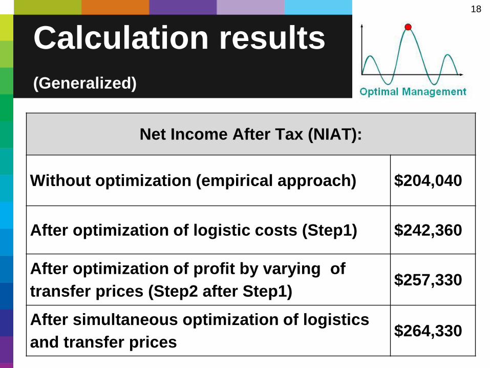
Calculation results
(Generalized)
Net Income After Tax (NIAT):
Without optimization (empirical approach) $204,040
After optimization of logistic costs (Step1) $242,360
After optimization of profit by varying of
transfer prices (Step2 after Step1) $257,330
After simultaneous optimization of logistics
and transfer prices $264,330
19
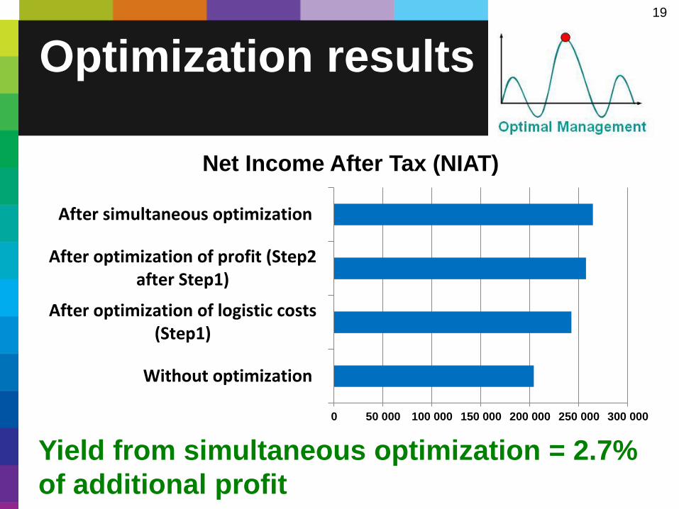
Optimization results
Yield from simultaneous optimization = 2.7%
of additional profit
0 50 000 100 000 150 000 200 000 250 000 300 000
Without optimization
After optimization of logistic costs(Step1)
After optimization of profit (Step2after Step1)
After simultaneous optimization
Net Income After Tax (NIAT)

20
• The more advanced the supply chain (more
goods positions and more nodes in the
chain), the greater the effect of
simultaneous optimization of flow of goods
and transfer prices.
• For an advanced supply chain (more goods
positions and more nodes in the chain),
you can’t do optimization calculation using
Excel.
The specificity of
Problem

21
Solution as a
service While product is being developed, we offer solution as a
service. The entire service process consists of the following steps:
• Research of basic structure of customer’s supply chain
• Estimation of costs on calculation and full data gathering
• Approval for parameters to be taken into account
• Fitting of the math model to the client’s needs
• Gathering all necessary data for the developed model
• Transformation of gathered data into computational model
• Performing the calculation
• Applying the results
By analogy to the tasks of logistics optimization, static model
calculates parameters for 18 months ahead every 6 months.
Dynamic model calculates weekly or monthly.

22
Contacts
Contact persons:
• In USA & Great Britain – Vitaliy Baklikov
phone: +1 240 620 1229
e-mail: [email protected]
• In Russia & CIS – Andrey Sukhobokov
phone: +7 903 577 9667
e-mail: [email protected]