Simultaneous Mapping and Stereo Extrinsic

Parameter Calibration Using GPS Measurements

Jonathan Kelly†, Larry H. Matthies∗ and Gaurav S. Sukhatme†

Abstract—Stereo vision is useful for a variety of robotics tasks,such as navigation and obstacle avoidance. However, recovery ofvalid range data from stereo depends on accurate calibrationof the extrinsic parameters of the stereo rig, i.e., the 6-DOFtransform between the left and right cameras. Stereo self-calibration is possible, but, without additional information, theabsolute scale of the stereo baseline cannot be determined. Inthis paper, we formulate stereo extrinsic parameter calibrationas a batch maximum likelihood estimation problem, and useGPS measurements to establish the scale of both the scene andthe stereo baseline. Our approach is similar to photogrammetricbundle adjustment, and closely related to many structure frommotion algorithms. We present results from simulation experi-ments using a range of GPS accuracy levels; these accuracies areachievable by varying grades of commercially-available receivers.We then validate the algorithm using stereo and GPS dataacquired from a moving vehicle. Our results indicate that theapproach is promising.

I. INTRODUCTION

Stereo vision is a rich sensing modality that is able provide

dense bearing, range and appearance information. However,

recovery of accurate range data from stereo, which is required

for metric mapping and in some cases for path planning

and obstacle avoidance, depends on careful calibration of the

extrinsic parameters that define the transform between the

stereo cameras. Calibration is typically carried out offline,

using a specialized calibration target with known geometry.

The need for precision calibration limits our ability to

build power-on-and-go robotic systems in which stereo is the

primary sensor. Further, although stereo self-calibration (auto-

calibration) is possible, it is well known that information about

the absolute scale of the translation between the cameras

cannot be obtained without external measurements, i.e., the

length of the stereo baseline is a free parameter [1].

In contrast to stereo, which is primarily useful for short-

range navigation, wide-area navigation systems such as GPS

can supply positioning information over the entire globe. Com-

modity GPS receivers have become cheap and ubiquitous, and

with the removal of selective availability, the accuracy of these

This work was funded in part by the US NSF (grants IIS-1017134 andCCF-0120778) and by a gift from the Okawa Foundation. Jonathan Kellywas supported by an Annenberg Fellowship from the University of SouthernCalifornia and by an NSERC doctoral postgraduate scholarship from theGovernment of Canada.

†Jonathan Kelly and Gaurav S. Sukhatme are with the Department ofComputer Science, University of Southern California, Los Angeles, California90089, {jonathsk,gaurav}@usc.edu.

∗Larry H. Matthies is with the Jet Propulsion Laboratory, CaliforniaInstitute of Technology, Pasadena, California 91109, lhm@jpl.nasa.gov.

receivers has improved dramatically. It should be possible

to leverage GPS for a variety of tasks beyond positioning.

In this paper we ask the following question: can we use

GPS and image feature measurements alone to calibrate the

extrinsic parameters of a robot-mounted stereo camera rig,

while the robot is operating? We seek a metric calibration

of the parameters, with a known scale factor.

To answer this question, we present a theoretical approach

and simulation studies and experiments which characterize

the feasibility of using GPS for calibration. We formulate

the calibration problem using a batch maximum likelihood

framework, in which point landmarks are viewed from mul-

tiple camera poses. Information about the absolute scale of

the scene and the stereo baseline is derived entirely from

GPS measurements. The calibration algorithm also produces

a map of the landmarks in the environment — this allows

calibration to be performed as part of a larger mapping task.

Our simulation results are based on trajectory data acquired

from a Pioneer 2-AT robot with an on-board GPS receiver.

Although we focus on the use of GPS here, the algorithm

we describe can be adapted for use with any sensor that is

able to provide coarse, wide-area three-dimensional position

measurements.

The remainder of the paper is organized as follows. We

review related work in Section II below. In Section III, we

formally define the calibration problem and motivate our

approach. Section IV discusses our methods for landmark

position and robot pose initialization, while Section V details

the maximum likelihood calibration algorithm. We describe

our simulation studies and vehicle experiments in Sections

VI and VII, respectively, and present results in Section VIII.

Finally, we offer some conclusions and directions for future

work in Section IX.

II. RELATED WORK

The problem of camera calibration has been studied exten-

sively in the photogrammetry community, with work dating

to the 1940s [2]. Much of the early research focused on

calibration for, e.g., aerial mapping, where the necessary level

of precision demands the use of sophisticated calibration

equipment. The algorithmic techniques, such as bundle ad-

justment [3], developed for these applications have now been

adopted by computer vision researchers.

Close-range self-calibration of both the intrinsic and extrin-

sic parameters of a stereo rig is demonstrated by Zhang, Luong

2011 IEEE International Conference on Robotics and AutomationShanghai International Conference CenterMay 9-13, 2011, Shanghai, China

978-1-61284-380-3/11/$26.00 ©2011 IEEE 279

280

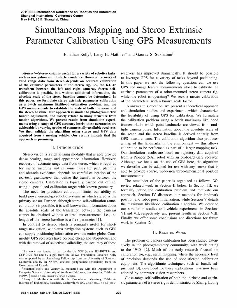
the camera frame relative to the world frame. The transform

from the right camera to the left camera is represented by the

6× 1 vector

vR =[

tL TR

L

RΘT

]T, (2)

where the 3×1 vector tL

Rdefines the translation of the right

camera optical center relative to the left camera optical center,

and the vector L

RΘ defines the orientation of the right camera

frame relative to the left camera frame.

We concatenate the landmark positions and left camera

poses together with the right-to-left camera transform and the

GPS-to-left camera translation to build the complete parameter

vector

X =[

tL TG

vTR

uT1 . . . uT

n pW Tl1

. . . pW Tlm

]T, (3)

where tL

Gis the 3 × 1 vector that defines the translation of

the GPS antenna in the left camera frame. The size of the

complete parameter vector is 9+6n+3m. Note that all of the

entries in the vector are static quantities which do not depend

on time.

We parameterize orientations using a minimal set of three

Euler angles. Although there are singularities in this repre-

sentation, constraints on the motion of the platform prevent

us from reaching any of the singular configurations (e.g., the

pitch and roll of a land vehicle are typically limited to ±15degrees).

B. Camera Sensor Model

We use an ideal projective (pinhole) model for both the

left and right cameras, and assume that the intrinsic and lens

distortion parameters are known.1 To compute the predicted

image measurements, we begin by expressing the position of

the ith landmark, at position pW

liin the world frame, in the

left and right camera frames

pLj

li= CT (W

LjΘ)( pW

li− tW

Lj), (4)

pRj

li= CT (L

RΘ)

(

CT (WLjΘ)( pW

li− tW

Lj)− tL

R

)

. (5)

Here, C(Θ) is a direction cosine (rotation) matrix, parame-

terized by the vector Θ of Euler angles.

Measurements zLj

liand z

Rj

liare the projections of the

ith landmark onto the left and right camera image planes,

respectively, from the jth left camera pose:

zLj

li=

[

uL

ij

vL

ij

]

=

[

xL

ij/ zL

ij

yL

ij/ zL

ij

]

+ ηij ,

xL

ij

yL

ij

zL

ij

= (KL) p

Lj

li,

(6)

zRj

li=

[

uR

lij

vR

lij

]

=

[

xR

ij/ zR

ij

yR

ij/ zR

ij

]

+ ηij ,

xR

ij

yR

ij

zR

ij

= (KR) p

Rj

li,

(7)

1We plan to explore full calibration of the both the intrinsic and extrinsicstereo parameters in future work.

where[

uij , vij]T

is the vector of observed left (resp. right)

horizontal and vertical image coordinates, K is the 3 × 3camera intrinsic parameter matrix, and ηij is a 2 × 1 white

Gaussian measurement noise vector with covariance matrix

Wij .

C. GPS Sensor Model

Each GPS measurement gives the position of the receiver in

the world frame. Accounting for the moment arm of the GPS

antenna relative to the left camera optical center, we have

zGj = tW

Lj+C(W

LjΘ) tL

G+ nj (8)

where nj is a 3 × 1 white Gaussian noise vector with

covariance matrix Sj .

This model neglects gross systematic errors due to multipath

interference. The occurrence of these types of errors is largely

dependent on the operating environment. To avoid incorporat-

ing pose measurements that include systematic errors, a chi-

squared distribution test can be used to reject GPS fixes that

lie outside of a specific confidence ellipsoid, based on the

measurement covariance [13]. Also, for non-holonomic vehi-

cles such as the Pioneer 2-AT robot, constraints on plausible

motions may be used as an additional validation gate for the

GPS data — e.g., we typically drive slowly and we know

a priori that the robot cannot move significantly in a lateral

direction over a short time interval.

IV. LANDMARK POSITION AND ROBOT POSE

INITIALIZATION

The batch calibration approach described in Section V is

only valid for small-residual problems, in which the initial

parameter values are reasonably close to their true values. In

particular, if there are large errors in the estimates of one

or more landmark positions, the calibration algorithm can

converge to the wrong solution, or diverge and fail to provide

an answer. The success of the algorithm therefore depends on

acquiring good initial landmark and camera pose estimates.

We use triangulation in combination with a maximum disparity

heuristic to determine the initial landmark positions; camera

pose estimates are derived from GPS data. The initialization

techniques are described below.

A. Maximum Disparity Initialization

Estimating the camera-relative depth of a landmark in the

environment using stereo normally involves some form of

triangulation. However, distance values derived from triangu-

lation are significantly affected by small errors in the estimated

orientation of either the left or the right camera; these small

orientation errors can produce very large errors in an estimated

landmark position. The problem is most severe for landmark

that lie far from the stereo rig.

We attempt to reduce the effects of triangulation errors using

a maximum disparity heuristic. Disparity is a measure of the

difference in the projected positions of the landmark on the left

281

and right camera image planes. For a fronto-parallel camera

configuration, the horizontal disparity of landmark point i is

dij = uR

ij − uL

ij (9)

where uR

lijand uL

lijare the projected horizontal image

coordinates for the landmark in the right and left cameras,

respectively; the disparity value is a negative quantity. For a

given, fixed left horizontal image coordinate, landmarks with

larger absolute disparity will be located nearer to the cameras.

Most stereo cameras will not, in general, be aligned in a

perfectly fronto-parallel configuration, and our initial estimate

of the camera pose will have some amount of error (otherwise

there would be no need for calibration). However, we can still

use our knowledge of the approximate relative pose of the

cameras, and of the horizontal disparity, to produce a rough

estimate of the landmark position. This approximation is poor

for small disparities, but reasonably good for large disparities.

Our approach is to delay initializing the position of land-

mark i until we find the left camera pose for which the left-

right horizontal disparity is the largest possible, relative to all

poses where the landmark is visible. We further constrain the

image plane points to lie within a fixed horizontal distance

of the principal point, which is less than the full size of the

image plane. This prevents initialization using points which

lie at the edges of the left or right image plane (in our

current implementation, points must lie within 250 pixels of

the principal point, on either side). We then triangulate the

left camera-relative the position of the landmark. The result

is that, in the majority of cases, the position of the landmark

is initialized when the robot and the landmark are in close

proximity, and the initial estimate of the landmark position

is reasonably close to the true position. This technique can

still fail, however, in cases where one or more landmarks lie

far from all of the camera poses (and the maximum disparity

value is small); we discuss this issue further in Section VI.

B. Initial Pose Estimation and Landmark Triangulation

The calibration algorithm requires an initial estimate of

the left camera pose at the time each GPS measurement

is acquired. We initialize the left camera position using the

available GPS fix and an approximate GPS antenna translation

vector (from, e.g., hand measurements or CAD data etc.). This

gives the translation of the left camera relative to the origin

of the world frame, but in general GPS does not provide

reliable information about the heading of the robot. For a non-

holonomic platform (such as the Pioneer 2-AT), and assuming

that the left camera optical axis is approximately aligned with

the longitudinal axis of the robot, we can estimate heading

using a line segment joining the positions defined by two GPS

measurements spaced closely in time.2 Because GPS altitude

data is usually less accurate than the horizontal positioning

information, we assume that the optical axis of camera is

initially horizontal.

2Here we also assume that the robot moves slowly, so that its trajectory isapproximately linear between GPS updates.

Fig. 2. Pioneer AT-2 with µBlox LEA-5H GPS unit, configured for datalogging experiments on the USC campus. The GPS antenna is visible at thecenter of the aluminum crossbeam.

For camera pose j, the initial 3D positions of the visible

landmarks (which have maximum disparity at pose j) are then

found by stereo triangulation, using the technique described

in [14]. Given a pair of corresponding left and right image

point measurements, zLj

liand z

Rj

li, we back-project rays

from the left and right camera optical centers through the

image plane points. If the image plane measurements were

error-free, these rays would intersect at a 3D single point,

however noise and matching errors inevitably cause the rays

to diverge. Instead, we find the midpoint of the shortest

perpendicular segment connecting the rays. This midpoint is

selected as the initial landmark position, after transforming

from the left camera frame to the world frame. More recently,

we have also explored the use of an inverse depth-based

parameterization for landmark positions, to better represent

the landmark position uncertainty [15].

V. CALIBRATION ALGORITHM

We use a batch iterated maximum likelihood formulation for

the complete calibration problem, in which we simultaneously

solve for the landmark positions, left camera poses, translation

of the GPS antenna, and the extrinsic calibration parameters.

First, we stack the image plane and GPS measurements to

form the complete observation vector

Z =[

zL1 T

l1z

R1 Tl1

. . . zLn Tlk

zRn Tlk

zG1 T . . . zGn T

]T

.

(10)

The value k is the index of the last landmark visible from

pose n. The observation covariance matrices for the image

plane and GPS measurements are, respectively,

W =

W11 · · · 02×2

.... . .

...

02×2 · · · Wkn

, S =

S1 · · · 03×3

.... . .

...

03×3 · · · Sn

. (11)

The complete observation covariance matrix is then

Σ =

[

W 0

0 S

]

. (12)

282

Note that, because the image and GPS measurements are

independent and uncorrelated, the covariance matrix is block

diagonal and can be inverted quickly.

We define the parameter and observation error vectors as,

respectively,

δX = X− X, δZ = Z− Z. (13)

where X is the current estimated parameter vector and Z is the

predicted observation vector based on X.3 The update step of

the iterated maximum likelihood algorithm involves linearizing

about the current parameter estimate, and we therefore require

the Jacobians of the image plane and GPS measurements with

respect to the pose and calibration parameters. The Jacobians

of an image plane point with respect to the ith landmark

position and the jth left camera pose are computed as

Hzli,pli

=

∂ zLj

li

∂pli

∂ zRj

li

∂pli

, Hzli,uj

=

∂ zLj

li

∂uj

∂ zRj

li

∂uj

. (14)

The Jacobian of an image plane point with respect to the

right camera extrinsic parameters, the Jacobian of a GPS

measurement with respect to the jth left camera pose, and

the Jacobian of a GPS measurement with respect to the GPS

translation parameters are

Hzli,vR

=∂ z

Rj

li

∂vR

, Huj=

∂ zGj

∂uj

, HtG =∂ zGj

∂ tL

G

. (15)

The complete Jacobian matrix H is formed by inserting

the partial derivative matrices above at the appropriate row

and column positions.4 Matrix H is sparse and block diag-

onal except for the first nine columns – as such, operations

involving H are amenable to optimization using sparse matrix

multiplication techniques.

The maximum likelihood estimate for the parameters is

obtained by iteratively performing a Levenberg-Marquardt

update, solving the system

(HTΣ−1H+ λ · diag(HTΣ−1H)) δX = HTΣ−1δZ. (16)

Here, λ is a damping factor which controls the direction of

motion along the parameter error surface; larger values of

λ force the update more towards gradient descent [3]. The

updated estimate for the parameter vector at iteration i is

Xi+1 = Xi + δXi. (17)

This process is iterated until convergence. We determine

that the estimate has converged when the two-norm of the

difference between the six extrinsic parameters over consec-

utive iterations is less than a small positive constant, ǫ (in

our implementation, ǫ = 10−6). If, on iteration i + 1, the

squared observation error increases relative to iteration i, we

3Estimated quantities are denoted with theˆ(hat) symbol.4For brevity, we omit the complete Jacobians. The Jacobians with respect to

the camera poses are particularly complex because the measurement involvesdivision by the camera-relative landmark depth.

−15 −10 −5 0 5 10 15

−15

−10

−5

0

5

10

15

Easting (m)

Nort

hin

g (

m)

Fig. 3. Robot trajectory (dashed blue line) with overlaid synthetic pointlandmarks (green dots). The complete trajectory is approximately 79 metersin length. A total of 225 landmarks are visible from 229 camera poses. Theyellow triangles indicate the estimated orientation of the robot and left cameraat various positions along the trajectory.

update the damping factor as λnew = 10λold and repeat the

iteration using the previous parameter estimate. Otherwise, we

decrease λ by a factor of 10 and continue; this is a standard

heuristic used in Levenberg-Marquardt optimization. As a last

step, we determine the maximum likelihood parameter vector

by performing an update with λ = 0.

VI. SIMULATION STUDIES

To evaluate the performance of the calibration algorithm, we

initially performed a series of simulation experiments using a

combination of real and synthetic data. We drove a Pioneer

2-AT robot equipped with an on-board µBlox LEA-5H GPS

receiver [16] in an open area on the USC campus, while

logging GPS and wheel odometry data in real time. The update

rates for GPS and odometry were 1 Hz and approximately

10 Hz, respectively. Total length of the trajectory was 79.3

m as measured by wheel odometry. The odometry data was

used only to verify that there were no gross errors in the GPS

measurements.

Based on the area covered by the (real) trajectory of the

robot, we then generated a set of 240 landmark points at

random positions on an annulus with an inner radius of 5

meters and an outer radius of 13 meters, and with random

heights between -0.5 and 0.5 meters. We used this trajectory

and set of synthetic landmark points, shown in Figure 3, as

ground truth for our simulations.

For each simulation trial, we captured a pair of simulated

images from the stereo cameras at every position along the

trajectory for which a GPS fix was available. After projecting

all visible landmarks into both the left and right image planes,

we added independent, zero-mean Gaussian noise with a

standard deviation of 1.0 pixels to the image coordinates,

to simulate errors in feature localization. Each (simulated)

283

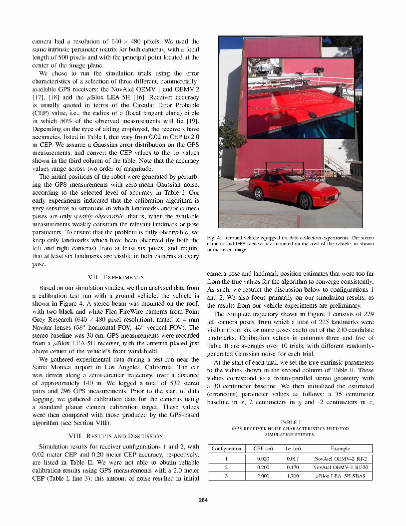
284

TABLE IIRIGHT CAMERA EXTRINSIC PARAMETER CALIBRATION RESULTS FOR GPS

RECEIVER CONFIGURATIONS 1 AND 2.

Configuration 1 Configuration 2

Parameter Truth Average σ Average σ

x (mm) 300.0 299.3 0.6 297.2 4.7

y (mm) 0.0 1.4 0.2 -0.4 0.5

z (mm) 0.0 3.6 0.3 21.1 3.4

Roll α (mdeg) 0.0 0.4 0.1 0.1 0.2

Pitch β (mdeg) 0.0 -1.9 0.1 -1.3 0.4

Yaw γ (mdeg) 0.0 1.5 0.1 0.2 0.1

with 2 degrees of positive roll and yaw error, and 4 degrees of

negative pitch error, i.e. with the cameras verged by 4 degrees.

The results show that, for both configurations, the average

residual camera orientation error after calibration is on the

order of one millidegree in roll, pitch and yaw. This is to be

expected, as camera rotation errors have a large effect on the

estimated landmark positions, and the batch estimator must

therefore drive the orientation errors close to zero to obtain a

low overall residual error. Indeed, we observed exactly this

behavior over sequential iterations of batch algorithm: the

rotation parameters typically converged first, followed by the

translation parameters.

The average residual errors for the translation parameters

are somewhat larger. For configuration 1, the average error is

less than 4 millimeters along all axes. This result, however,

depends on a level of GPS accuracy that can only be achieved

by real-time carrier-phase differential receivers – at present,

these units are very expensive and their deployment is limited.

For configuration 2, the average residual error is less than

3 millimeters in x and y – along the x direction, the error

is less than 6% of the original error value at the start of

the simulation. The average residual error along the z axis is

larger than along the other axes, however, and slightly larger

on average than the initial error introduced at the start of

the simulation. Achieving better calibration results for the ztranslation parameter may simply be a matter of collecting

more data. We are exploring this issue.

In analyzing our results, we noted that accurate stereo

calibration can sometimes be obtained even when there are

relatively large errors in the 3D positions of several landmarks.

This is because the calibration algorithm minimizes image re-

projection error — for landmarks that are visible from a small

number of clustered poses only, and that lie at a significant

distance from the cameras in all cases, the reprojection error

is relatively insensitive to landmark depth.

Our simulation results are based on incremental GPS mea-

surements that are acquired as the robot or vehicle moves,

navigating or performing some other activity. It is possible

to obtain more accurate positioning information simply by

remaining stationary and filtering a large amount of GPS data.

This increased accuracy comes at the expense of the additional

time, however, which may be unacceptable in some situations.

TABLE IIIRIGHT CAMERA EXTRINSIC PARAMETER CALIBRATION RESULTS FOR

VEHICLE EXPERIMENT.

Parameter Target-Based Value GPS-Based Value

x (mm) 298.2 293.1

y (mm) 2.6 4.6

z (mm) 2.9 13.6

Roll α (deg) -0.12 -0.14

Pitch β (deg) 0.14 0.15

Yaw γ (deg) -0.74 -0.72

Results for our experiment with the test vehicle are also

in agreement with the values determined using the standard

target-based calibration procedure, as shown in Table III. We

note that, in practice, when a large number of GPS satellites

are in view, the µBlox LEA-5H receiver is able to obtain

position fixes with an accuracy significantly better than 2.0

m CEP. We are presently conducting additional experiments

to determine the performance of the algorithm under a wider

variety of conditions.

IX. CONCLUSIONS AND FUTURE WORK

This paper presented an approach for calibrating a robot-

or vehicle-mounted stereo rig, using GPS measurements to

determine the absolute scale of the scene and of the stereo

baseline. This work is a step towards developing robots that

can operate for long periods of time without requiring manual

sensor re-calibration.

Our results are promising: we obtained reasonable cali-

bration accuracy using GPS measurements with a CEP of

up to 0.2 meters. A CEP of 0.2 meters approaches the

accuracy available with standard differential GPS, which is

readily available in many locations. The batch algorithm

establishes a benchmark for other approaches — we believe

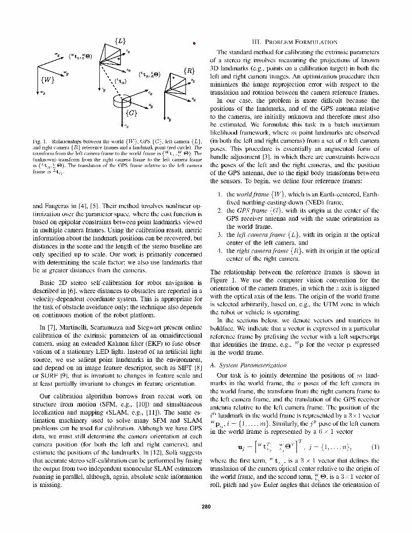
Fig. 5. Example left stereo camera image acquired during one vehiclecalibration experiment.

285

that incremental solutions, which incorporate larger numbers

of observations over time, should be able to improve upon

these results. Further, as the global satellite navigation network

grows to incorporate the Russian GLONASS and European

Galileo constellations, we can expect even better positioning

accuracy from commodity receivers. Also, the algorithm we

have described is not limited to GPS — it can be adapted

for use with other sensors that provide positioning or ranging

information.

There are several directions for future work. We are cur-

rently exploring the use of a combination of wheel odometry

and GPS measurements to perform full calibration of both

the intrinsic and extrinsic parameters of the stereo rig. Based

on the batch solution, we are also developing an alternative,

sequential estimator formulation. Lastly, we would like to de-

fine optimal or near-optimal robot trajectories that enable rapid

calibration in the field, based on the uncertainty associated

with each calibration parameter.

REFERENCES

[1] R. Hartley and A. Zisserman, Multiple View Geometry in Computer

Vision, 2nd ed. Cambridge: Cambridge University Press, Nov. 2003.[2] C. McGlone, E. Mikhail, and J. Bethel, Manual of Photogrammetry,

5th ed. American Society for Photogrammetry and Remote Sensing,July 2004.

[3] B. Triggs, P. McLauchlan, R. Hartley, and A. W. Fitzgibbon, “BundleAdjustment – A Modern Synthesis,” in Vision Algorithms: Theory

and Practice, ser. Lecture Notes in Computer Science, B. Triggs,A. Zisserman, and R. Szeliski, Eds. Springer-Verlag, Jan. 2000, vol.1883, ch. 21, pp. 298–372.

[4] Z. Zhang, Q.-T. Luong, and O. Faugeras, “Motion of an UncalibratedStereo Rig: Self-Calibration and Metric Reconstruction,” INRIA SophiaAntipolis, Tech. Rep. 2079, Oct. 1993.

[5] ——, “Motion of an Uncalibrated Stereo Rig: Self-Calibration and Met-ric Reconstruction,” in Proc. 12th IAPR Int’l Conf. Pattern Recognition

(ICPR’94), vol. 1, Oct. 1994, pp. 695–697.

[6] R. A. Brooks, A. M. Flynn, and T. Marill, “Self Calibration of Motionand Stereo Vision for Mobile Robot Navigation,” Massachusetts Instituteof Technology, Cambridge, USA, Tech. Rep. AIM-984, Aug. 1987.

[7] A. Martinelli, D. Scaramuzza, and R. Siegwart, “Automatic Self-Calibration of a Vision System during Robot Motion,” in Proc. IEEE

Int’l Conf. Robotics and Automation (ICRA’06), Orlando, USA, May2006, pp. 43–48.

[8] D. G. Lowe, “Distinctive Image Features from Scale-Invariant Key-points,” Int’l J. Computer Vision, vol. 2, no. 60, pp. 91–110, Nov. 2004.

[9] H. Bay, T. Tuytelaars, and L. V. Gool, “SURF: Speeded Up Robust Fea-tures,” in Computer Vision – ECCV 2006, ser. Lecture Notes in ComputerScience, A. Leonardis, H. Bischof, and A. Pinz, Eds. Springer Berlin/ Heidelberg, 2006, vol. 3951, pp. 404–417.

[10] A. Chiuso, P. Favaro, H. Jin, and S. Soatto, “Structure from MotionCausally Integrated Over Time,” IEEE Trans. Pattern Analysis and

Machine Intelligence, vol. 24, no. 4, pp. 523–535, Apr. 2002.[11] S. Thrun, “Robotic Mapping: A Survey,” Carnegie Mellon University,

Pittsburgh, USA, Tech. Rep. CMU-CS-02-111, Feb. 2002.[12] J. Sola, “Multi-camera VSLAM: from former information losses to

self-calibration,” in Proc. IEEE/RSJ Int’l Conf. Intelligent Robots and

Systems Workshop on Visual SLAM: An Emerging Technology, SanDiego, USA, Oct./Nov. 2007.

[13] S. Sukkarieh, E. M. Nebot, and H. F. Durrant-Whyte, “A High IntegrityIMU/GPS Navigation Loop for Autonomous Land Vehicle Applica-tions,” IEEE Trans. Robotics and Automation, vol. 15, no. 3, pp. 572–578, June 1999.

[14] Y. Cheng, M. W. Maimone, and L. Matthies, “Visual Odometry on theMars Exploration Rovers,” in Proc. IEEE Int’l Conf. Systems, Man and

Cybernetics, vol. 1, Big Island, USA, Oct. 2005, pp. 903–910.[15] J. M. M. Montiel, J. Civera, and A. J. Davison, “Unified Inverse Depth

Parametrization for Monocular SLAM,” in Proc. Robotics: Science and

Systems (RSS’06), Philadelphia, USA, Aug. 2006.[16] uBlox AG, “LEA-5 u-blox 5 Modules for GPS and GALILEO,”

datasheet, Jan. 2008. [Online]. Available: http://www.u-blox.com/en/lea-5a.html

[17] NovAtel Inc., “NovAtel OEMV-1 GPS Receiver,” datasheet, Jan. 2008.[Online]. Available: http://www.novatel.com/products/gnss-receivers/oem-receiver-boards/oemv-receivers/

[18] ——, “NovAtel OEMV-2 GPS+GLONASS Receiver,” datasheet,Jan. 2008. [Online]. Available: http://www.novatel.com/products/gnss-receivers/oem-receiver-boards/oemv-receivers/

[19] J. A. Farrell and M. Barth, The Global Positioning System & Inertial

Navigation, 1st ed. McGraw-Hill, Dec. 1998.

286