Simulink Model of an Induction MachineThis document describes the defining equations for a dynamic induction machinemodel to be implemented in Simulink. There are a number of research publica-tions on this topic however they often lack key pieces of information which theauthor either decided were so self-evident they need not be included or just ne-glected due to their familiarity with the subject matter. Something that may beabout to happen again.

In terms of research into the design and control of electrical machines the processdescribed here is “classical” (i.e. more than a few years old). In practice anumber of companies known to the author use a process similar to this for severaltypes of machine drive but with additions to accommodate effects particularto their application. For example in high speed work the frictional heating ofthe rotor due to wind-age and aerodynamic losses may be included as theseare often a function of speed. Saturation of the machine iron may be includedby parameterising the leakage and mutual inductances as a function of flux orcurrent. Copper and Eddy current losses are relatively easily added and thereafterthe thermal effects that these create may be included as well. The final form of thesimulation and its scope is limited only by technical necessity, the human resourceavailable to perform the development work and the financial cost the developeris prepared to incur to possess the simulation. The main cost of developing asimulation for a machine is the validation stage(s) which require physical space,test equipment and human resources to gather the validation data. By comparisonthe programming of the model including the HR costs of the programming andthe cost of the software is often a minor component of a project.

Figure 1: Per phase equivalent circuit of an induction machine.

The three phase induction machine per phase equivalent model which is com-monly taught to undergraduates is shown in fig. 1. A discursive introduction tomachines and control may be found in [1]. Some common questions that under-graduates might face involve referring the rotor to the stator side and derivingthe torque equation, the pull out torque, the starting torque and sketching a

1

Bear Instruments Ltd August 2018

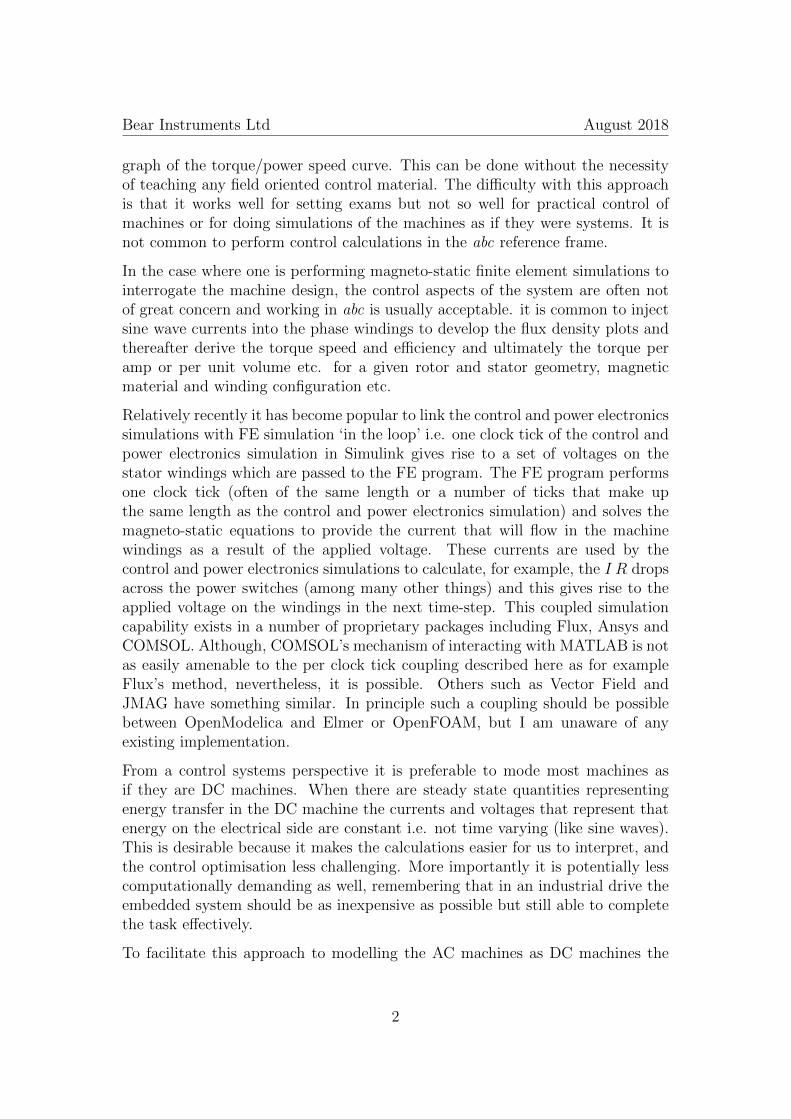
graph of the torque/power speed curve. This can be done without the necessityof teaching any field oriented control material. The difficulty with this approachis that it works well for setting exams but not so well for practical control ofmachines or for doing simulations of the machines as if they were systems. It isnot common to perform control calculations in the abc reference frame.

In the case where one is performing magneto-static finite element simulations tointerrogate the machine design, the control aspects of the system are often notof great concern and working in abc is usually acceptable. it is common to injectsine wave currents into the phase windings to develop the flux density plots andthereafter derive the torque speed and efficiency and ultimately the torque peramp or per unit volume etc. for a given rotor and stator geometry, magneticmaterial and winding configuration etc.

Relatively recently it has become popular to link the control and power electronicssimulations with FE simulation ‘in the loop’ i.e. one clock tick of the control andpower electronics simulation in Simulink gives rise to a set of voltages on thestator windings which are passed to the FE program. The FE program performsone clock tick (often of the same length or a number of ticks that make upthe same length as the control and power electronics simulation) and solves themagneto-static equations to provide the current that will flow in the machinewindings as a result of the applied voltage. These currents are used by thecontrol and power electronics simulations to calculate, for example, the I R dropsacross the power switches (among many other things) and this gives rise to theapplied voltage on the windings in the next time-step. This coupled simulationcapability exists in a number of proprietary packages including Flux, Ansys andCOMSOL. Although, COMSOL’s mechanism of interacting with MATLAB is notas easily amenable to the per clock tick coupling described here as for exampleFlux’s method, nevertheless, it is possible. Others such as Vector Field andJMAG have something similar. In principle such a coupling should be possiblebetween OpenModelica and Elmer or OpenFOAM, but I am unaware of anyexisting implementation.

From a control systems perspective it is preferable to mode most machines asif they are DC machines. When there are steady state quantities representingenergy transfer in the DC machine the currents and voltages that represent thatenergy on the electrical side are constant i.e. not time varying (like sine waves).This is desirable because it makes the calculations easier for us to interpret, andthe control optimisation less challenging. More importantly it is potentially lesscomputationally demanding as well, remembering that in an industrial drive theembedded system should be as inexpensive as possible but still able to completethe task effectively.

To facilitate this approach to modelling the AC machines as DC machines the

2

Bear Instruments Ltd August 2018

work of Clark and Park is used either in the Clarke Park transform or the dqtransform. This transform converts the three phase currents of the stationary abcframe to the stationary α, β reference frame and then to the rotating d-q referenceframe. If a refresher is needed then there is an excellent video at https://www.

youtube.com/watch?v=vdeVVTltr1M (not one of mine and I’m not affiliated withthe author). The transformation may be performed easily in Simulink using abuilt in block. It is not necessary to describe the transform mathematics here, itmay be found in textbooks including [2–4]. A discussion of PWM techniques canbe found in [5] and [6].

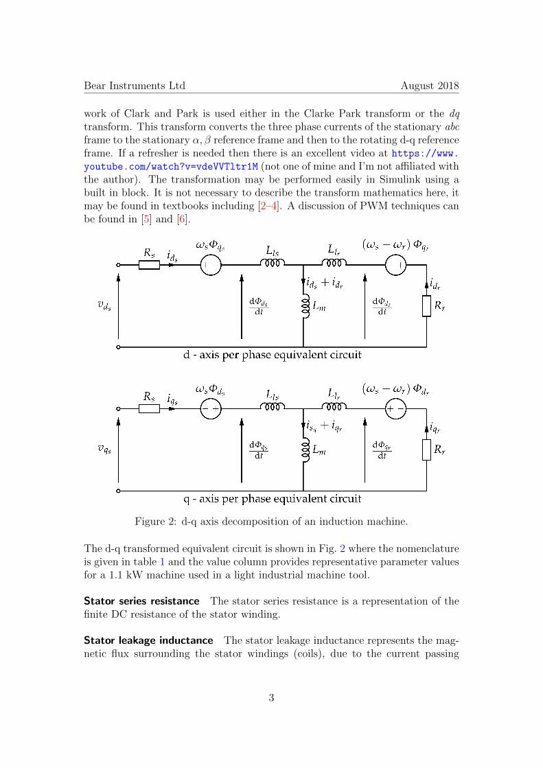
Figure 2: d-q axis decomposition of an induction machine.

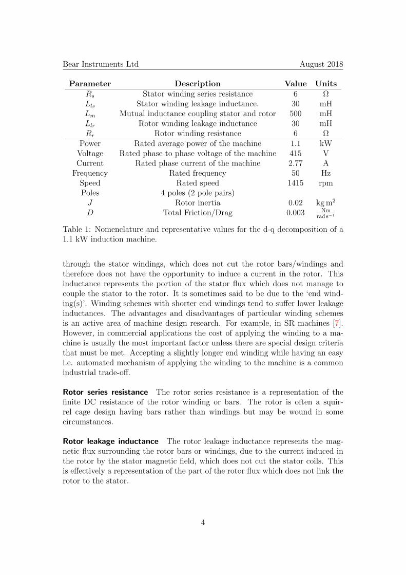
The d-q transformed equivalent circuit is shown in Fig. 2 where the nomenclatureis given in table 1 and the value column provides representative parameter valuesfor a 1.1 kW machine used in a light industrial machine tool.

Stator series resistance The stator series resistance is a representation of thefinite DC resistance of the stator winding.

Stator leakage inductance The stator leakage inductance represents the mag-netic flux surrounding the stator windings (coils), due to the current passing

3

Bear Instruments Ltd August 2018

Parameter Description Value UnitsRs Stator winding series resistance 6 ΩLls Stator winding leakage inductance. 30 mHLm Mutual inductance coupling stator and rotor 500 mHLlr Rotor winding leakage inductance 30 mHRr Rotor winding resistance 6 Ω

Power Rated average power of the machine 1.1 kWVoltage Rated phase to phase voltage of the machine 415 VCurrent Rated phase current of the machine 2.77 A

Frequency Rated frequency 50 HzSpeed Rated speed 1415 rpmPoles 4 poles (2 pole pairs)J Rotor inertia 0.02 kg m2

D Total Friction/Drag 0.003 Nmrad s−1

Table 1: Nomenclature and representative values for the d-q decomposition of a1.1 kW induction machine.

through the stator windings, which does not cut the rotor bars/windings andtherefore does not have the opportunity to induce a current in the rotor. Thisinductance represents the portion of the stator flux which does not manage tocouple the stator to the rotor. It is sometimes said to be due to the ‘end wind-ing(s)’. Winding schemes with shorter end windings tend to suffer lower leakageinductances. The advantages and disadvantages of particular winding schemesis an active area of machine design research. For example, in SR machines [7].However, in commercial applications the cost of applying the winding to a ma-chine is usually the most important factor unless there are special design criteriathat must be met. Accepting a slightly longer end winding while having an easyi.e. automated mechanism of applying the winding to the machine is a commonindustrial trade-off.

Rotor series resistance The rotor series resistance is a representation of thefinite DC resistance of the rotor winding or bars. The rotor is often a squir-rel cage design having bars rather than windings but may be wound in somecircumstances.

Rotor leakage inductance The rotor leakage inductance represents the mag-netic flux surrounding the rotor bars or windings, due to the current induced inthe rotor by the stator magnetic field, which does not cut the stator coils. Thisis effectively a representation of the part of the rotor flux which does not link therotor to the stator.

4

Bear Instruments Ltd August 2018

Stator back EMF The d axis stator back EMF is proportional to the syn-chronous speed and the q axis flux. The current gives rise to a magnetic fluxand the rate of change of that magnetic flux gives rise to a voltage across thewinding in which the current flows the back EMF will act to oppose the changein current (Lenz’s law). If the current is sinusoidal the voltage that develops willbe co-sinusoidal (derivative of sine is cosine) cosine may be thought of as a sinewave with a phase shift of π/4. Since the d and q axes are perpendicular toeach-other (shifted π/4 radians) the EMF felt on the d axis is due to the q axisflux and similarly the EMF felt on the q axis is proportional to the d axis flux.

Rotor back EMF The d axis rotor back EMF is proportional to the differencebetween the synchronous speed and the rotor speed (i.e. the “slip”) and the rotorflux generated by the q axis. The difference in the synchronous and rotor speedis the rate at which the stator field appears to be moving past us if we’re sittingon the rotor bars looking radially outwards.

Figure 2 also notes the voltage across the stator windings (Lls + Lm) and rotorwindings (Llr + Lm) is given by the rate of change of flux cutting those windings.

Kirchhoff’s laws may be used to develop a set of loop equations for the stator androtor. Later these equations will be combined with flux equations to form a selfconsistent set of equations that Simulink (or Modelica) can solve. The mechanicalsystem will also be added to the simulation. Starting with the d axis stator loopand recalling that the voltage across an inductor is given by the product of therate of change of current and the inductance of the coil (v = L di/dt),

vds − idsRs + ωs Φqs − Llsd idsdt

− Lmd

dt(ids + idr) = 0 (1)

The relationship between flux and current (flux is the product of inductance andcurrent) can be used to simplify (1), although this can be obtained by using thevoltages marked by the rate of change of flux in fig. 2 as well

vds − idsRs + ωs Φqs −d Φds

dt= 0 (2)

transposing (2) to make d Φds

dtthe subject,

d Φds

dt= vds − idsRs − ωs Φqs (3)

The expressions involving differential equations are usually cast in the form ofderivative = everything else, because that is the way the Simulink blocks willbe arranged. After the equation is formed the 1/s block is used to integratethe differential equation. The differential equations are coupled and the solver

5

Bear Instruments Ltd August 2018

that Simulink calls will solve them simultaneously. Well, presuming the solutionconverges. If the simulation doesn’t converge it’s quite likely that one of theequations is either derived incorrectly or has not been transferred into Simulinkcorrectly. For the q axis,

d Φqs

dt= vqs − iqsRs + ωs Φds (4)

The rotor loops can be similarly treated, starting with the d axis,

d Φdr

dt= −idr Rr − (ωs − ωr) Φqr (5)

and for the q axis,d Φqr

dt= −iqr Rr + (ωs − ωr) Φdr (6)

Four expressions link the d and q axis rotor and stator flux starting with the qaxis stator flux,

Φsq = (iqs + iqr) Lm + iqs Lls (7)

for the d axis stator flux,

Φsd = (ids + idr) Lm + ids Lls (8)

for the q axis rotor flux,

Φrq = (iqs + iqr) Lm + iqr Llr (9)

for the d axis rotor flux,

Φrd = (ids + idr) Lm + idr Llr (10)

In this case the flux equations may be written in terms of the d and q axis cur-rents. This is necessary because the simulation will proceed by a voltage beingimpressed on the stator winding. This voltage will be used to calculate the rateof change of flux, which in turn will be integrated to obtain that flux. The fluxwill then be used to calculate the current. The current will be fed back into acontrolled current source which exists between (i.e. in parallel with) the termi-nals across which the voltage was originally impressed. It’s possible to formulateanother approach in which a current is impressed and the resulting EMF on thestator is calculated (along with all the mechanical outputs) however this requiresthe system of equations to be cast in terms of calculating derivatives. Takingderivatives in numerical sampled data systems is potentially risky because it is anoisy process which can promote instability (i.e. lack of convergence). Integra-tion or numerical quadrature is by comparison a low noise and generally stableapproach. There are some circuit reasons to use an integration approach as well.

6

Bear Instruments Ltd August 2018

When the simulation is set up with some power electronics the machine modelwill take the calculated current independent of the other effects in the system.If a back EMF approach was used the converter supply voltage would have themachine terminal voltage subtracted from it and the machine current would bewhatever flowed through the series resistance of the power semiconductor device.If the power device model has no series resistance and the link voltage was aperfect voltage source there will be an over-constrained matrix in the simulationas two voltage sources will have been connected in parallel which is undesirable.Keeping in mind all the foregoing, if the converter design under considerationis a current source converter or an impedance source converter it’s not impossi-ble, it may even be desirable, to cast the machine model as being a controlledvoltage device. However, in voltage source inverter applications, which are muchmore common, presenting the machine model to the power electronics model asa controlled current device is certainly preferable. This should be clearer whenconsidered in association with the video demonstrating the Simulink code (seehttps://youtu.be/wM72tarF_to).

The q axis stator flux expression (7) becomes,

iqs =Φqs − Lm iqrLm + Lls

(11)

Equation (8) is transposed to provide the d axis stator current,

ids =Φds − Lm idrLm + Lls

(12)

Two more expressions are require and can be derived trivially from (9) and (10)to provide the d and q axis rotor currents in terms of the d and q axis rotorflux. Looking at (11) and (12) it is clear that the solution of these two equationsand the two which are not written out must be simultaneous as they all dependon each-other. This is similar to the differential equations for flux, they areinterdependent and the solver must solve them all simultaneously.

The electro-mechanical torque can be expressed as,

Te =3

2

P

2(iqs ((ids + idr) Lm) + ids ((iqs + iqr) Lm)) (13)

The electro-mechanical torque could be expressed in terms of flux more simplybut the Simulink model that this document relates to uses the form presentedhere. Since the integral of the time derivative of flux is calculated prior to thecurrent the Simulink blocks flow in a more aesthetic way if the current is used todevelop the torque. The rate of change of speed is given by,

dωr

dt=Te −Dωr − TL

J(14)

7

Bear Instruments Ltd August 2018

where ωr is the rotor angular velocity in rad s−1, Te is the electro-mechanicaltorque in Nm, D is the frictional drag in Nm/(rad s−1), TL is the load torque,Nm (which when positive opposes the electro-mechanical torque) and J is thetotal mechanical inertia of the rotating parts in kg m2. The position of the rotor,in radians, is the integral of the rotor angular velocity,

θ =

∫ωr dt. (15)

The implementation in Simulink is presented in a video at https://youtu.be/

wM72tarF_to

About the Author

Dr. James Green runs Bear Instruments Ltd, an electronicsengineering consultancy specialising in analogue, mixed signaland power electronics systems design. James was lecturerin electrical machines and controls in the Department ofElectronic and Electrical Engineering at the Universityof Sheffield from 2013 – 2018 and was Royal Academyof Engineering Industrial Teaching Fellow from 2017 –2018. He gained his PhD in 2012 in semiconductor devicecharacterisation and has since worked on academic researchand industrial design problems in, among other fields,microwave curing of composite materials and automotivebattery testing and modelling. www.bearinstruments.co.uk

8

Bear Instruments Ltd August 2018

References

[1] A. Hughes, Electric Motors and Drives Fundamentals, Types and Applica-tions, third edition ed., 2006.

[2] B. K. Bose, Power Electronics and Motor Drives: Advances and Trends. El-sevier, 2006.

[3] N. Mohan, Advanced Electric Drives. Wiley, 2014.

[4] F. Giri, AC Electric Motors Control. Wiley, 2013.

[5] N. Mohan, First Course on Power Electronics and Drives. MNPERE, 2003.

[6] E. C. dos Santos Jr. and E. R. C. da Silva, Advanced Power Electronic Con-verters, ser. IEEE Press Series on Power Engineering, M. E. El-Hawary, Ed.,2015.

[7] X. Y. Ma, G. J. Li, G. W. Jewell, and Z. Q. Zhu, “Recent development of re-luctance machines with different winding configurations, excitation methods,and machine structures,” CES Transactions on Electrical Machines and Sys-tems, vol. 2, no. 1, pp. 82–92, March 2018. doi: 10.23919/TEMS.2018.8326454

9