simulations of preindustrial, present-day, and 2100 conditions in … · 20 interactions important...

Simulations of preindustrial, present-day, and 2100

conditions in the NASA GISS composition and climate

model G-PUCCINI

D. T. Shindell, G. Faluvegi, N. Unger, E. Aguilar, G. A. Schmidt, D. M.

Koch, S. E. Bauer, R. L. Miller

To cite this version:

D. T. Shindell, G. Faluvegi, N. Unger, E. Aguilar, G. A. Schmidt, et al.. Simulations ofpreindustrial, present-day, and 2100 conditions in the NASA GISS composition and climatemodel G-PUCCINI. Atmospheric Chemistry and Physics Discussions, European GeosciencesUnion, 2006, 6 (3), pp.4795-4878. <hal-00301540>

HAL Id: hal-00301540

https://hal.archives-ouvertes.fr/hal-00301540

Submitted on 15 Jun 2006

HAL is a multi-disciplinary open accessarchive for the deposit and dissemination of sci-entific research documents, whether they are pub-lished or not. The documents may come fromteaching and research institutions in France orabroad, or from public or private research centers.

L’archive ouverte pluridisciplinaire HAL, estdestinee au depot et a la diffusion de documentsscientifiques de niveau recherche, publies ou non,emanant des etablissements d’enseignement et derecherche francais ou etrangers, des laboratoirespublics ou prives.

https://hal.archives-ouvertes.fr

https://hal.archives-ouvertes.fr/hal-00301540

ACPD6, 4795–4878, 2006

Composition andclimate modelingwith G-PUCCINI

D. T. Shindell et al.

Title Page

Abstract Introduction

Conclusions References

Tables Figures

J I

J I

Back Close

Full Screen / Esc

Printer-friendly Version

Interactive Discussion

EGU

Atmos. Chem. Phys. Discuss., 6, 4795–4878, 2006www.atmos-chem-phys-discuss.net/6/4795/2006/© Author(s) 2006. This work is licensedunder a Creative Commons License.

AtmosphericChemistry

and PhysicsDiscussions

Simulations of preindustrial, present-day,and 2100 conditions in the NASA GISScomposition and climate modelG-PUCCINID. T. Shindell1,2, G. Faluvegi1,2, N. Unger1,2, E. Aguilar1,2, G. A. Schmidt1,2,D. M. Koch1,3, S. E. Bauer1,2, and R. L. Miller1,4

1NASA Goddard Institute for Space Studies, New York, NY, USA2Center for Climate Systems Research, Columbia University, NY, USA3Dept. of Geophysics, Yale University, New Haven, USA4Dept. of Applied Physics and Applied Math, Columbia University, NY, USA

Received: 3 February 2006 – Accepted: 13 March 2006 – Published: 15 June 2006

Correspondence to: D. T. Shindell ([email protected])

4795

http://www.atmos-chem-phys-discuss.net

http://www.atmos-chem-phys-discuss.net/6/4795/2006/acpd-6-4795-2006-print.pdf

http://www.atmos-chem-phys-discuss.net/6/4795/2006/acpd-6-4795-2006-discussion.html

http://www.copernicus.org/EGU/EGU.html

ACPD6, 4795–4878, 2006



Title Page



Tables Figures

J I

J I

Back Close

Full Screen / Esc



EGU

Abstract

A model of atmospheric composition and climate has been developed at the NASAGoddard Institute for Space Studies (GISS) that includes composition seamlessly fromthe surface to the lower mesosphere. The model is able to capture many features of theobserved magnitude, distribution, and seasonal cycle of trace species. The simulation5

is especially realistic in the troposphere. In the stratosphere, high latitude regions showsubstantial biases during period when transport governs the distribution as meridionalmixing is too rapid in this model version. In other regions, including the extrapolartropopause region that dominates radiative forcing (RF) by ozone, stratospheric gasesare generally well-simulated. The model’s stratosphere-troposphere exchange (STE)10

agrees well with values inferred from observations for both the global mean flux andthe ratio of Northern to Southern Hemisphere downward fluxes.

Simulations of preindustrial (PI) to present-day (PD) changes show troposphericozone burden increases of 11% while the stratospheric burden decreases by 18%.The resulting tropopause RF values are −0.06 W/m2 from stratospheric ozone and15

0.40 W/m2 from tropospheric ozone. Global mean mass-weighted OH decreases by16% from the PI to the PD. STE of ozone also decreased substantially during this time,by 14%. Comparison of the PD with a simulation using 1979 pre-ozone hole conditionsfor the stratosphere shows a much larger downward flux of ozone into the tropospherein 1979, resulting in a substantially greater tropospheric ozone burden than that seen in20

the PD run. This implies that reduced STE due to Antarctic ozone depletion may haveoffset as much as 2/3 of the tropospheric ozone burden increase from PI to PD. How-ever, the model overestimates the downward flux of ozone at high Southern latitudes,so this estimate is likely an upper limit.

In the future, the tropospheric ozone burden increases sharply in 2100 for the A1B25

and A2 scenarios, by 41% and 101%, respectively. The primary reason is enhancedSTE, which increases by 71% and 124% in the two scenarios. Chemistry and dry de-position both change so as to reduce ozone, partially in compensation for the enhanced

4796





ACPD6, 4795–4878, 2006



Title Page



Tables Figures

J I

J I

Back Close

Full Screen / Esc



EGU

STE. Thus even in the high-pollution A2 scenario, and certainly in A1B, the increasedozone influx dominates the burden changes. However, STE has the greatest influenceon middle and high latitudes and towards the upper troposphere, so RF and surface airquality are dominated by emissions. Net RF values due to projected ozone changesdepend strongly on the scenario, with 0.1 W/m2 for A1B and 0.8 W/m2 for A2. Changes5

in oxidation capacity are also scenario dependent, with values of plus and minus sevenpercent in the A2 and A1B scenarios, respectively.

1 Introduction

There are many ways in which changes in atmospheric composition and climate arecoupled. The interactions are especially pronounced in the case of chemically reactive10

gases and aerosols. For example, atmospheric humidity increases as climate warms,altering reactions involving water vapor and aqueous phase chemistry in general, whichin turn affects the abundance of radiative active species such as ozone and sulfate. Ad-ditional couplings exist via climate-sensitive natural emissions, such as methane fromwetlands and isoprene from forests, aerosol-chemistry-cloud interactions in a chang-15

ing climate, and large-scale circulation shifts in response to climate change, such asstratosphere-troposphere exchange (STE). This paper presents the latest version ofthe NASA Goddard Institute for Space Studies (GISS) composition and climate modelas part of our continuing efforts to more realistically simulate the range of physicalinteractions important to past, present and future climates.20

The trace gas photochemistry has been expanded from the earlier troposphere-onlyscheme described in Shindell et al. (2003) to include gases and reactions important inthe stratosphere. At the same time, the sulfate aerosol and trace gas chemistry havebeen fully coupled (Bell et al., 2005) and interactions between chemistry and mineraldust have been added to the model. Climate-sensitive emissions have been included25

for methane from wetlands, NOx from lightning, dust from soils, and DMS from theocean. Water isotopes and a passive linearly increasing tracer have been included,

4797





ACPD6, 4795–4878, 2006



Title Page



Tables Figures

J I

J I

Back Close

Full Screen / Esc



EGU

allowing better transport diagnostics. All components have been developed within thenew GISS ModelE climate model (Schmidt et al., 2006). Since the climate model de-veloped under the ModelE project has been named GISS model III, and the chemistryis also the third major version of its development following Shindell et al. (2001, 2003),it is appropriate to call this model the GISS composition and climate model III. We pre-5

fer, however, a more descriptive name: the GISS model for Physical Understanding ofComposition-Climate INteractions and Impacts (G-PUCCINI).

We present a detailed description of the model in Sect. 2, followed by an evaluationagainst available observations in Sect. 3. Section 4 presents the response to preindus-trial and 2100 composition and climate changes as an initial application of this model.10

We conclude with a discussion of the model’s successes and limitations with an eyetowards determination of the suitability of the current model for various potential futurestudies.

2 Model description

2.1 Trace gas and aerosol chemistry15

The trace gas photochemistry has been expanded from the tropospheric scheme de-veloped previously (Shindell et al., 2003) to include species and reactions importantin the stratosphere. Table 1 lists the molecules included in the gas photochemistry.Table 2 presents the additional 78 new reactions incorporated within the chemistryscheme. Together with the reactions included previously, the photochemistry now in-20

cludes 155 reactions. Rate coefficients are taken from the NASA JPL 2000 handbook(Sander et al., 2000). Photolysis rates are calculated using the Fast-J2 scheme (Bianand Prather, 2002), except for the photolysis of water and nitric oxide (NO) in theSchumann-Runge bands, which are parameterized according to Nicolet (1984), Nico-let and Cieslik (1980).25

Heterogeneous chemistry in the stratosphere follows the reactions listed in Table 2.

4798





ACPD6, 4795–4878, 2006



Title Page



Tables Figures

J I

J I

Back Close

Full Screen / Esc



EGU

Aerosol surface areas are set to match those used in the GCM’s calculation of radia-tive transfer based upon an updated version of the volcanic plus background aerosoltimeseries of Sato et al. (1993). For all the simulations described here, we use thestratospheric aerosol distribution for 1984, a mid-range year in terms of volcanic load-ing. Surface areas for polar stratospheric clouds (PSCs) are set using simple tem-5

perature thresholds for type I and II particles, with a parameterization of sedimenta-tion also included. A more sophisticated model of particle growth based on Hansonand Mauersberger (1988) is being incorporated into the chemistry code, but is not yetfunctional. Thus the simulations do not include all potential pathways for interactionsbetween polar ozone chemistry and climate or emissions changes as PSC formation is10

not sensitive to water or nitric acid abundance variations. Given that the model’s trans-port biases limit the realism of its polar ozone simulations in any case, it was deemeda better use of resources to address this in future higher resolution runs than to repeatthese simulations with a more advanced PSC scheme.

Chemistry can be included in the full model domain, or it can be restricted to levels15

below the meteorological tropopause. In the latter case, climatological ozone is used inthe stratosphere and NOx is prescribed as a fixed fraction of the ozone abundance asin our previous models. While we focus on the full chemistry model, both configurationsare evaluated here so that future studies can select the most appropriate version. Forthe tropospheric chemistry-only version, the ozone climatology is set to 1990s levels.20

To better understand the model’s simulation of stratospheric transport, we have in-corporated a passive, linearly increasing tracer as a standard feature along with thechemical tracers. This tracer is initialized in the lowest model layer with a value thatincreases by one unit each year, with a linear interpolation used to set monthly values.The difference between the tracer value at a given point and the surface level value25

then gives the mean time in years since the air left the surface. By comparing valuesthroughout the stratosphere with those at the tropical tropopause, we can evaluate theage of air in the stratosphere and compare with observations of CO2 and SF6.

The updated modelE version of the sulfate and sea salt model is described and eval-

4799





ACPD6, 4795–4878, 2006



Title Page



Tables Figures

J I

J I

Back Close

Full Screen / Esc



EGU

uated in Koch et al. (2006). It includes prognostic simulations of DMS, MSA, SO2 andsulfate mass distributions. The mineral dust aerosol model transports four differentsizes classes of dust particles with radii between 0.1–1, 1–2, 2–4, and 4–8 microns.Particle sources are identified using the topographic prescription of (Ginoux, 2001). Di-rect dust emission increases with the third power of the wind speed above a threshold5

that increases with soil moisture. Emission is calculated by integrating over a probabil-ity distribution of surface wind speed that depends upon the speed explicitly calculatedby the GCM at each grid box, along with the magnitude of fluctuations resulting fromsubgrid circulations created by boundary layer turbulence, along with dry and moistconvection. As a result, emission can occur even if the GCM grid box wind speed is10

below the threshold, so long as there are subgrid fluctuations. Dust particles are re-moved from the atmosphere by a combination of gravitational settling, turbulent mixing,and wet scavenging. Dust also affects the radiation field, and can thus influence pho-tolysis rates. A more detailed description of the dust model, along with a comparisonto regional observations, is given by Miller et al. (2006) and Cakmur et al. (2006).15

The model includes heterogeneous chemistry for the uptake of nitric acid on mineraldust aerosol surfaces. This is described by a pseudo first-order rate coefficient whichgives the net irreversible removal rate of gas-phase species to an aerosol surface.We use the uptake coefficient of 0.1 recommended from laboratory measurements(Hanisch and Crowley, 2001), though this value is fairly uncertain.20

The model also includes the stable water isotopes HDO and H182 O, which are fully

coupled to the GCM’s hydrologic cycle. Comparison between the modeled and ob-served values of these isotopes, and especially of their vertical profiles, can be a use-ful way to evaluate (and improve) the stratosphere-troposphere exchange in the modeland the parameterization of cloud physics (Schmidt et al., 2005).25

For the simulations described here, the tropospheric chemistry-only simulations wererun including interactive aerosols, which are coupled to the chemistry (Bell et al., 2005).Heterogeneous chemistry on dust was included in a separate sensitivity study to iso-late its influence. In the full chemistry simulations, we revert to using offline prescribed

4800





ACPD6, 4795–4878, 2006



Title Page



Tables Figures

J I

J I

Back Close

Full Screen / Esc



EGU

aerosol fields for computational efficiency as the chemistry-aerosol coupling has a sub-stantial effect on the aerosol simulation, but only a minor effect on the trace gases,which are our primary concern here.

The model has the capability to have changes in composition affect radiative transferfor radiatively active species including ozone, methane, aerosols and dust. The full5

chemistry simulations were performed including such interactions. However, the simu-lations we report on here for model evaluation used prescribed present-day sea surfacetemperatures (SSTs) and sea ice conditions, so that changes in the radiatively activegases could not affect climate substantially, though they could influence atmospherictemperatures. In the climate simulations described in Sect. 4, however, this interaction10

becomes important.

2.2 Sources and sinks

Emissions of trace gases and aerosols are largely the same as those used in previousversions (Shindell et al., 2003). They include the standard suite of emissions from fos-sil fuel and biomass burning, soils, industry, livestock, forests, wetlands, etc. These are15

based largely on GEIA inventories (Benkovitz et al., 1996). Sulfur emissions are fromthe EDGAR inventory as described in Bell et al. (2005). For the new long-lived speciesincluded here, N2O and CFCs (and CO2), we prescribe values at observed amounts(Table 3) in the lowest model layer. This technique is also available for methane, thoughin the present-day simulations described here we use the full set of methane emissions.20

CFCs are modeled using the characteristics of CFC-11 but with a magnitude designedto capture the total chlorine source from all CFC species (i.e. each CFC yields onechlorine atom when broken down, so the amount of CFCs is set to match total anthro-pogenic chlorine). We also assume there is a background chlorine value of 0.5 ppbvfrom natural sources.25

4801





ACPD6, 4795–4878, 2006



Title Page



Tables Figures

J I

J I

Back Close

Full Screen / Esc



EGU

2.3 Climate model

During the past several years, primary GISS modeling efforts have been directed intoan entirely rewritten and upgraded climate model under the modelE project (Schmidt etal., 2006). This resulting GISS model, called either modelE or model III, incorporatespreviously developed physical processes within a single standardized structure quite5

different from the older model. This structure is much more complicated to create, butmakes the interaction between GISS model components easier and more physicallyrealistic. The standardization across components has also allowed many improve-ments to be included relatively easily. An example is that the previous schemes allcalculated momentum in somewhat different ways. With modelE’s uniform treatment of10

momentum, it was quickly apparent that momentum was not conserved in the interac-tion between the gravity-wave drag scheme and the rest of the circulation, which hasnow been corrected.

ModelE also includes several advances compared to previous versions, includingmore realistic physics and improved convection and boundary layer schemes. The15

horizontal resolution can be easily altered, unlike previous versions. Standard diagnos-tics include statistical comparisons with satellite data products such as ISCCP cloudcover, cloud height, and radiation products, MSU temperatures, TRMM precipitation,and ERBE radiation products. Over a full suite of evaluation comparisons, includingthe satellite data and standard reference climatologies for parameters such as circula-20

tion, precipitation, snow cover, and water vapor, modelE now substantially outperformsall other GISS model versions (of course not on every individual quantity), producingrms errors approximately 11% less than those for Model II’. The new modelE GCMwas used for the GISS simulations performed for the forthcoming IntergovernmentalPanel on Climate Change (IPCC) Fourth Assessment Report (AR4). Hence this model25

has been scrutinized in great detail, so that the behavior of physical processes havebeen compared with a wide range of observations and the model’s response to a largenumber of forcings has been well-characterized.

4802





ACPD6, 4795–4878, 2006



Title Page



Tables Figures

J I

J I

Back Close

Full Screen / Esc



EGU

An important new feature of modelE for the trace gas and aerosol species is a care-fully constructed cloud tracer budget. Most, if not all, chemical and aerosol models(including all pre-modelE GISS models) do not save dissolved species in a cloud bud-get but instead return the dissolved (unscavenged) species to the model grid box atthe end of each model time-step. In our model, we have created a cloud liquid bud-5

get and this has important implications for tracer distributions. Inclusion of the cloudtracer budget decreases sulfate production in the clouds (since most of the sulfate isultimately rained out instead of released back to the grid box) (Koch et al., 2006) andreduces the abundance of soluble O3 precursors, such as nitric acid (HNO3), whichwere systematically overestimated in previous models. We have also developed a new10

dry deposition module within modelE that is physically consistent with the other surfacefluxes (e.g. water, heat) in the planetary boundary layer scheme of the GCM, which wasnot the case in earlier models (or indeed in most chemistry-climate models).

Yet another important feature of modelE is the capability to run the GCM with linearrelaxation, or “nudging”, to reanalysis data for winds. This allows the model’s mete-15

orology to be forced to match fairly closely that which existed during particular times,making for a much cleaner comparison with observational datasets.

GISS model development has benefited particularly from the close interaction of thecomposition modelers with the basic climate model developers at all stages, which hasenabled development of many consistent physical linkages such as the surface fluxes20

and liquid tracer budgets. Here we use a version with 23 vertical layers (model topin the mesosphere at 0.01 hPa) and 4×5 degree horizontal resolution. Present-daysimulations use seasonally varying climatological sea surface temperatures and seaice coverage representative of the 1990s (Table 3).

4803





ACPD6, 4795–4878, 2006



Title Page



Tables Figures

J I

J I

Back Close

Full Screen / Esc



EGU

3 Evaluation of present-day simulation

3.1 Long-lived gases in the stratosphere

Several long-lived species have been included as transported gases. These includenitrous oxide (N2O), a source of NOx radicals in the stratosphere, methane (CH4) andwater vapor (H2O), sources of stratospheric HOx, and chlorofluorocarbons (CFCs), a5

source of halogens. A linearly increasing tracer to diagnose transport was also in-cluded. This is presented in Fig. 1, which shows the age of air in the stratospherecalculated using the linearly increasing tracer in comparison with values derived fromSF6 and CO2 observations (Andrews et al., 1999; Boering et al., 1996; Elkins et al.,1996; Harnisch et al., 1996) and values from other models (Hall et al., 1999). Clearly10

the model’s air in the high latitude lower stratosphere is too young, a feature seen inmost GCMs and even in CTMs driven by assimilated meteorological data (Scheele etal., 2005; Schoeberl et al., 2003). The annual mean residual vertical velocity in themodel underestimates the maximum values seen in the UKMO analyses (Swinbankand O’Neill, 1994), and the region of upwelling extends too far poleward in the South-15

ern Hemisphere, and to a much lesser extent in the Northern Hemisphere (Fig. 2).The model’s mean upwelling velocity is 35% slower than in the observations. However,the seasonal cycle shows the maximum upwelling occurring in the summer subtrop-ics in both hemispheres, in accord with Rosenlof (1995) and Plumb and Eluszkiewicz(1999). This simulation of the seasonality of tropical upwelling is a marked improve-20

ment over that seen in the older GISS model II, which failed to reproduce the australsummer maximum entirely (Butchart et al., 20061). The model also simulates a localminimum in upwelling near the equator, a feature seen in most GCMs but not in pre-vious GISS models (Butchart et al., 20061). The underestimate of upwelling velocitiesindicates that air reaches the high latitude lower stratosphere too easily via merid-25

1Butchart, N., Scaife, A. A., Bourqui, M., et al.: A multi-model study of climate change in theBrewer-Dobson circulation, Clim. Dyn., submitted, 2006.

4804





ACPD6, 4795–4878, 2006



Title Page



Tables Figures

J I

J I

Back Close

Full Screen / Esc



EGU

ional transport across the semi-permeable barriers in the stratosphere rather than viaa Brewer-Dobson circulation that is too rapid.

Consistent with these circulation biases, the model’s N2O and CH4 distributions aretoo broad compared with satellite climatologies from the Halogen Occultation Experi-ment (HALOE) and the Cryogenic Limb Array Etalon Spectrometer (CLAES) (Randel5

et al., 1998) (Fig. 3). Also, the high mixing ratio values entering the stratosphere in thetropics do not penetrate to high enough altitudes before being chemically transformed.The distribution of CFCs in the model exhibits a similar shape. The weak meridionalgradients in the distributions of these long-lived gases implies that transport acrossthe subtropical and polar barriers is too rapid. Additionally, there may not be enough10

downward transport within the polar vortex, as seen near the North Pole in Fig. 3. Thisappears to result from the underestimate of polar isolation which keeps the polar re-gion from cooling as much as it should, rather than biases in the overturning circulationgiven that the age of air is too short in the polar regions. In the interest of space, weconcentrate on results for April, a month showing a “typical” ozone distribution neither15

too close to the solstices nor drastically affected by polar heterogeneous chemistry.The distributions are similarly too broad in other months.

The model’s water vapor distribution in the stratosphere closely resembles the op-posite of the methane distribution up through ∼1 hPa. However, the water vapor nearthe tropical tropopause entry point is too low, leading to a negative bias throughout the20

stratosphere. Given the extremely high sensitivity of water vapor to temperature andconvective mixing in this region, the bias in water reflects only a small underestimate oftemperature or overestimate of convective drying. As in observations, values increaseby roughly 3 ppmv from the tropical tropopause to the upper stratosphere at 2 hPa.However, the model’s meridional gradients in stratospheric water are again too weak25

and the stratopause region water values are too low, both features being consistentwith the circulation-induced biases in the methane distribution. Water vapor mixing ra-tios decrease below 5.5 ppmv at about 0.2–0.3 hPa, as in observations, however thismesospheric loss takes place at all latitudes in the model but only near the springtime

4805





ACPD6, 4795–4878, 2006



Title Page



Tables Figures

J I

J I

Back Close

Full Screen / Esc



EGU

pole in observations. This may indicate that chemistry above the model top influencesthose layers, or that the current parameterization of mesospheric photolysis needs tobe improved. Future work will explore this region further. The seasonality of watervapors entry into the stratosphere is simulated reasonably well, with a clear “tropicaltape recorder” signal seen in the water vapor distribution (Schmidt et al., 2005).5

3.2 Ozone

The model’s annual cycle of column ozone and the difference with respect to observa-tions is shown in Fig. 4. The simulated distribution shows a broad minimum and littleseasonality in the tropics, with greater ozone values and a larger seasonal cycle at highlatitudes, in good agreement with observations. However, the model underestimates10

the magnitude of the seasonal cycle at high northern latitudes, with too little ozoneduring the winter and too much ozone during the summer, and has a general positivebias over the Antarctic. The model’s column ozone is within 10% of the observed valuethroughout the tropics and subtropics and over most mid-latitude areas. High latitudedifferences are larger, in excess of 20% in some locations during some seasons.15

There are two primary reasons for the high latitude biases apparent in Fig. 4. Duringthe summer, high latitude temperatures in the ModelE GCM without chemistry exhibita cold bias of ∼10◦C in the lowermost stratosphere (Schmidt et al., 2006). By slowingdown the rates of ozone destroying reactions, this contributes to an increasing positiveozone biases during summer and fall seen in both hemispheres. The second reason20

is that the model’s transport of gases into high latitudes is in general too rapid in thelower stratosphere, with the subtropical and polar barriers being too permeable, as dis-cussed in Sect. 3.1. This transport bias contributes to the underaccumulation of ozonein the Arctic during winter, and to the failure of the model to simulate lower ozonevalues over the Antarctic than at Southern Hemisphere mid-latitudes during fall and25

winter, in both cases as air is not confined closely enough within the polar region. Themodel does produce a fairly reasonable Antarctic ozone hole. The timing is consistentwith observations, as is the depletion relative to the wintertime values, though the min-

4806





ACPD6, 4795–4878, 2006



Title Page



Tables Figures

J I

J I

Back Close

Full Screen / Esc



EGU

imum values are too large as those winter starting values are too large (as discussedpreviously).

Figure 5 presents the April zonal mean ozone distribution in the model and from theMicrowave Limb Sounder (MLS) and HALOE instruments. Clearly the Arctic distribu-tion is too closely centered around 10 hPa, similar to middle latitudes, consistent with5

an underestimate of downward transport within the polar vortex and too much mixingacross the vortex boundary. The Southern Hemisphere polar vortex similarly showstoo much ozone from about 10–5 hPa and contours of large ozone mixing ratios thatextend too far poleward from the mid-latitude maximum. Ozone in the tropics is well-simulated, though the maximum ozone mixing ratio in the model is slightly less than10

in observations. In fact, the simulation is generally of high quality in regions whereozone’s photochemical lifetime is short, suggesting that the model’s chemistry schemeworks well and that biases are indeed largely related to transport.

In addition to examining the present-day stratospheric ozone climatology, sufficientdata exists to allow evaluation of the sensitivity of stratospheric ozone to perturbations.15

Observations from the Stratospheric Aerosol and Gas Experiment (SAGE) series ofsatellites have been used to calculate ozone trends over the period 1979 to 2004 (up-dated from Randel and Wu, 1999). We have performed a simulation using 1979 cli-mate and long-lived trace gas conditions (Table 3), and can then compare the modeledchange from 1979 to the present with these observations, as shown in Fig. 6. Note that20

our simulation did not include changes in emissions of short-lived tropospheric ozoneprecursors, as it was designed to isolate the impact of stratospheric ozone changes onthe atmosphere. Qualitatively, the model captures the pattern of local maxima in ozoneloss in both polar regions in the lowermost stratosphere and in the upper stratosphereand also simulates the local minimum in the tropical stratosphere around 25–30 km25

altitude. Quantitatively, the model’s ozone trends are typically a few percent larger thanthose seen in the satellite record. This is especially true in the Arctic lower strato-sphere, though the uncertainty in the observed trends is very large as variability is highin this region. In the Antarctic lower stratosphere, the model’s trend is in fairly good

4807





ACPD6, 4795–4878, 2006



Title Page



Tables Figures

J I

J I

Back Close

Full Screen / Esc



EGU

agreement with the magnitude calculated from observations, though the largest deple-tion extends over a larger area, especially down into the troposphere. However, thevalues in the troposphere and near the tropopause in general are all more negativein the model since these simulations did not include increases in tropospheric ozoneprecursors. As seen in the runs that did include such increases, the troposphere be-5

came more and more polluted during the twentieth century, which would account forthe positive trends send in the lowermost portion of the SAGE data at mid-latitudes andin the tropics and also the smaller negative values seen at high latitudes.

To evaluate the lowermost stratosphere and troposphere, where satellite climatolo-gies do not yet exist, we have extensively compared modeled annual cycles of ozone10

with a long-term balloon sonde climatology from remote sites (Logan, 1999). Annualcycles at several pressure levels are shown for selected sites in Fig. 7, while statisticalcomparisons with all sites are presented in Table 4. Results are included for simu-lations incorporating chemistry throughout the model domain and for simulations withtropospheric chemistry only. Values from the previous model II’ version are also shown15

in the table for comparison.The ozone values and annual cycles over a wide range of latitudes are reasonably

well simulated (Fig. 7). The high latitude biases evident in the previous analysis of thetotal column are immediately apparent at the uppermost sonde levels, however. Thefull chemistry version underpredicts wintertime ozone at 125 hPa at both Resolute and20

Hohenpeissenberg, and overpredicts at Lauder and especially at Syowa. Interestingly,the depth of the springtime ozone hole over Syowa is reproduced fairly reasonably.The biases have only a minor effect on lower altitudes at most locations, with the ex-ception of Syowa where they persist clearly through at least 500 hPa. The shape of theseasonal cycle is generally well reproduced in the model, with maximum and minimum25

values typically falling at the correct time of year. There is clearly an underestimateof ozone in the tropical upper troposphere at Natal, but this is not the case at otherlocations.

A broader comparison of all 16 ozonesonde sites, as shown in Table 4, demonstrates

4808





ACPD6, 4795–4878, 2006



Title Page



Tables Figures

J I

J I

Back Close

Full Screen / Esc



EGU

that the new composition and climate model gives a substantially improved simulationin comparison with the older model II’ tropospheric chemistry model. Running the newmodel in tropospheric chemistry-only mode leads to a better match with observations atall levels, though especially those away from the surface. Using the full chemistry cal-culation, inherently a more difficult endeavor compared with prescribing stratospheric5

ozone to exactly match observations, coincidentally leads to differences with respectto observations that are quite similar to those seen in the tropospheric chemistry-onlymodel II’. However, this implies that at a level such as 125 hPa, in the stratosphere formany of the sites, the full chemistry model does a much better job for the low latitudesites for which this level is in the troposphere (consistent with the modelE tropospheric10

chemistry-only performance). Transport from the stratosphere to the troposphere issubstantially improved in the new modelE, as evidenced by the improvement in the tro-pospheric chemistry modelE versus II’. Thus the large positive bias in the full chemistrymodel at 300 hPa does not result solely from excessive downward transport, a majorproblem in previous GISS GCMs. It is at least partially attributable to the overestimate15

of high latitude lower stratospheric ozone, especially in the Southern Hemisphere. Asimilar statistical comparison of the full chemistry run with sonde data leaving out thetwo high latitude sites Resolute and Syowa shows average differences in ppbv reducedfrom 34.7 to 23.7 at 300 hPa, from 45.7 to 37.0 at 200 hPa, and from 83.2 to 75.8 ppbvat 125 hPa, while at lower levels, there is little effect. This demonstrates that, as ex-20

pected, a fair amount of the discrepancy with observations arises from the model’s highlatitude biases. However, some excessive downward transport may still be occurring,which is partially masked in the tropospheric chemistry-only run by the negative biasat 200 hPa. The large 300 hPa positive bias is thus not present in the modelE tropo-spheric chemistry-only run. Aside from this large positive bias (31%), biases at other25

levels are generally quite small, with values of 12% or less (and often 3% or less) atall other levels for both the full chemistry and tropospheric chemistry-only simulations.The GISS tropospheric-only chemistry model participated in the ACCENT/IPCC AR4assessment of chemistry models, which included an evaluation of present-day simula-

4809





ACPD6, 4795–4878, 2006



Title Page



Tables Figures

J I

J I

Back Close

Full Screen / Esc



EGU

tions against this same ozonesonde climatology. In comparison with the other models,the GISS model performed quite well, with a root-mean-square (rms) error value of6.3 ppbv compared with a range of rms error values of 4.6 to 17.8 ppbv (Stevenson etal., 2006).

An additional simulation identical to the tropospheric chemistry-only run except in-5

cluding heterogeneous reactions on dust surfaces was also performed. The samestatistical comparison of ozone fields with sonde data for that run shows reductions inthe mean ozone concentration at those sites of 1.3% at 300 hPa, of 9.8% at 500 hPa,and of 1.0% at 950 hPa. Changes are 0.5% or less at 125 and 200 hPa. The reductionoccurs primarily via removal of nitric acid on dust surfaces (see Sect. 3.3), which re-10

duces the reactive nitrogen available for ozone production. The overall effect on ozoneis mixed, with minor improvements in the model-data comparison at some levels andminor reductions in quality at others. The effect of the model’s liquid tracer budget hasalso been assessed. The inclusion of liquid tracers leads to an overall reduction inozone due to enhanced removal of soluble species such as HNO3 (see Sect. 3.2). The15

tropospheric ozone burden is reduced by 10 Tg (3%). The changes are not uniform,however, with ozone generally decreasing in the upper troposphere but sometimesincreasing at lower levels. For example, in the same statistical comparison with son-des discussed above, the ozone concentration at those sites is reduced by 0.6 ppbv at300 hPa, but increased by 1.6 ppbv at 500 hPa. This results from enhanced downward20

transport of aqueous-phase HNO3 via advection and precipitation followed by evapora-tion. Overall the comparison with sondes generally changes by only about 1%, thoughat the 900 hPa level the difference between sondes and the model is reduced by ∼3%with the inclusion of the liquid tracer.

Surface ozone data is more widely available, and we compare modeled values with25

measurements from 40 sites using the climatology of Logan (1999), based on datafrom many sources (Cros et al., 1988; Kirchhoff and Rasmussen, 1990; Oltmans andLevy, 1994; Sanhueza et al., 1985; Sunwoo and Carmichael, 1994). The model doesa reasonably good job of matching the observed annual cycle at most sites, a sample

4810





ACPD6, 4795–4878, 2006



Title Page



Tables Figures

J I

J I

Back Close

Full Screen / Esc



EGU

of which is shown in Fig. 8. The results for the tropospheric chemistry-only simulationare fairly similar to those of our previous model (Shindell et al., 2003), consistent withthe 900 hPa results shown in Table 4. There is some improvement at Reykjavik owingto the improved downward transport at high latitudes. At Northern middle latitudes,the simulation at Rockport is substantially improved, while that in the Northeastern US5

is marginally better though the Hohenpeissenberg results are marginally worse. Thesurface ozone values in the full chemistry simulation are very similar to those in thetropospheric chemistry-only version, unsurprisingly. Interestingly, South Pole shows asubstantial difference, with more wintertime ozone in the full chemistry run. While thisimproves the agreement with observations, it results from the overestimate of ozone in10

the Antarctic lower stratosphere. This does indicate that the model correctly transportsstratospheric ozone anomalies all the way to the surface at South Pole. Comparingall 40 sites with the model’s values shows that the mean bias has decreased from+3.8 ppbv in model II’ to −1.4 ppbv in the tropospheric chemistry-only run and 0.6 ppbvin the full chemistry run. A correlation plot of the annual average surface ozone (Fig. 9),15

however, shows that there is still substantial scatter despite the small mean bias. Itis important to remember that the observations are primarily from remote sites, andthat the model’s 4 by 5 degree grid boxes tend to include a mix of remote and urbanlocations over most continental regions, making the comparison somewhat imperfect.

It thus appears that the model generally does a reasonable job of reproducing ob-20

servations throughout much of the atmosphere. The primary exception is the polarstratosphere, as discussed above, where values show biases up to about 25%. This isan important limitation, affecting the model’s usefulness in performing studies of polarozone depletion, though the Antarctic ozone hole is fairly well represented. However,the model reproduced observations in the extrapolar regions quite well, and shows25

especially good agreement near the surface and in the vicinity of the tropopause (Ta-ble 4). The latter is a key region for radiative forcing, and thus the results indicatethat the model is useful for studies of how composition-climate interactions may affectclimate and air quality.

4811





ACPD6, 4795–4878, 2006



Title Page



Tables Figures

J I

J I

Back Close

Full Screen / Esc



EGU

One area that has proved difficult to study in the past has been the response of STEto climate change. Without the inclusion of stratospheric chemistry, our previous stud-ies, and those of many other groups using tropospheric chemistry-only setups, werestrongly influenced by the definition of the upper boundary for chemistry. For example,if chemistry was calculated below a fixed level, part of the upper troposphere and low-5

ermost stratosphere, a region where data is sparse, had to be prescribed, and odd gra-dients could be created across this arbitrary chemical boundary. If instead chemistryfollowed the tropopause, changes in the location of the tropopause could dramaticallyaffect the results as ozone amounts changed from climatology to calculated values.This latter effect could create sources and sinks as a box was categorized alternately10

in one region then the other. The new full chemistry model avoids these problems,and so we explore the issue of STE in some depth in Sect. 4.4. In preparation for this,we give the tropospheric ozone budget for the models discussed here initially calcu-lating the terms for the atmosphere below 150 hPa and using fluxes across this level(Table 5).15

The tropospheric ozone burden of 379 Tg in the tropospheric chemistry-only modelis quite similar to the 349 Tg burden in the previous model II’ tropospheric chemistry-only version. These burdens are very close despite a large change in dry depositionbetween the two models that resulted from the switch between the earlier surface fluxcalculation to one consistent with other climate variables in the new modelE. This re-20

inforces the point we’ve made previously that only the STE value is reasonably wellconstrained from observations. These give a best estimate of 450 Tg/yr with a rangeof 200 to 870 Tg/yr for the cross-tropopause flux based on O3-NOy correlations (Mur-phy and Fahey, 1994), a range of 450–590 Tg/yr at 100 hPa from satellite observations(Gettelman et al., 1997), and a constraint from potential vorticity and ozone fluxes for25

the downward extrapolar flux (∼80–100% of total downward flux) of 470 Tg/yr for theyear 2000 (Olsen et al., 2003). Some analyses also provide estimates of the ratio ofNH to SH downward flux, with the NH contributing 55% of the total in Olsen et al. (2003)and 57% in (Gettelman et al., 1997). The present-day model results are in good agree-

4812





ACPD6, 4795–4878, 2006



Title Page



Tables Figures

J I

J I

Back Close

Full Screen / Esc



EGU

ment with this value, with 57% of the downward flux in the NH (Table 6). The total STEvalues in the tropospheric chemistry-only model are consistent with the observationalconstraints. The full chemistry simulation has a larger value that is on the high side ofthe range from observations, owing to the excessive downward ozone fluxes at highSouthern latitudes where ozone amounts are overestimated (the full chemistry STE5

value at 115 hPa, our closest level to 100 hPa, is 578 Tg/yr). The other budget termssimply respond to balance the tropospheric abundance as chemistry is typically veryrapid, making the system highly buffered and the other budget terms of limited valuefor model evaluation.

3.3 Nitrogen species10

The model’s distribution of HNO3 matches the location of maxima in the satellite ob-servations in both extratropical regions fairly well (Fig. 5). The area within the 9 ppbvcontour is too large in the SH, however. Nitric acid can be formed by heterogeneouschemistry, and is therefore dependent upon aerosol and PSC surface areas and a pa-rameterization of particle growth and sedimentation. Since these are quite simple in15

this model, it is not surprising that the abundance of HNO3 does not match perfectlywith observations. In the tropics, the level with maximum HNO3 occurs too low, consis-tent with the tropical upward transport being too slow and mixing across the subtropicsbeing too rapid.

In the troposphere, the nitric acid simulation is in good qualitative agreement with20

the limited available data, and is quantitatively much improved over previous resultsdespite still being too large. Figure 10 shows nitric acid profiles from troposphericchemistry-only simulations performed with and without the inclusion of heterogeneouschemistry on dust, and for a run without the use of the liquid tracer budget. Theseare compared with a variety of aircraft measurements (Emmons et al., 2000). In the25

new simulations with or without heterogeneous chemistry on dust, the overestimate ofHNO3 typically seen in our earlier model II’ results has been reduced substantially inthe new modelE, primarily as a result of the inclusion of a liquid tracer budget. The

4813





ACPD6, 4795–4878, 2006



Title Page



Tables Figures

J I

J I

Back Close

Full Screen / Esc



EGU

presence of a liquid tracer, allowing dissolved species to remain in the condensedphase for multiple timesteps, leads to global reductions in the abundance of solublegases, with an overall reduction in the global HNO3 burden of 5% and a reductionin the tropospheric ozone burden of 3%, as noted previously. The effect of the liquidbudget is much larger for sulfur-containing species, some of whose burdens decreased5

by 25–30% (Koch et al., 2006). In some locations where liquid water is abundant andlong-lasting, quite large reductions occur (e.g. Japan in Fig. 10). Additionally, it is clearfrom the figure that heterogeneous chemistry on dust further improves the results inmany locations (though not all). The overall model improvement is especially striking forJapan, where the liquid tracer and the removal of nitric acid on dust particles blowing10

out from the Asian interior brings the modeled values down to observed levels. Incontrast, profiles from model II’ or modelE without the liquid tracers or dust chemistrywere roughly a factor of 5 too large in this area, while those from the modelE run withoutdust chemistry are a factor of 2 to 3 too large.

Similar comparisons of the vertical profiles of NOx and PANs in the troposphere15

show good agreement between the model and observations in most locations (notshown), similar to that seen in our previous model (Shindell et al., 2003). Analysis of themodeled NOx simulation in the stratosphere is complicated by the fact that the availableclimatologies from HALOE record sunrise and sunset NO and NO2, but these specieschange rapidly during these times. The model’s monthly mean April NOx shows a peak20

of ∼12–13 ppbv in the tropics at ∼5 hPa, in reasonable agreement with the sum of NOand NO2 in the HALOE sunrise measurements but somewhat lower than the sunsetsum which is peaks at ∼18 ppbv. Given that the model values are a diurnal average,it seems reasonable that they should lie below some of the sunlit observations. Sincenitrogen oxide abundances change so rapidly during sunrise and sunset, even a more25

detailed comparison with the model results is likely to be inconclusive owing to themodel’s half hour chemistry timestep.

The global annual average source of NOx from lightning is 5.2 Tg N/yr in both thetropospheric chemistry-only and the full chemistry models. This source is calculated

4814





ACPD6, 4795–4878, 2006



Title Page



Tables Figures

J I

J I

Back Close

Full Screen / Esc



EGU

internally based on the GCM’s convection using parameterizations for total and cloud-to-ground lightning modified from (Price et al., 1997). The spatial distribution of light-ning agrees fairly well with observations (Boccippio et al., 1998), especially over landareas (Fig. 11). The model tends to overestimate lightning over SE Asia and Indone-sia, however. This leads to overestimates of the total flash rate of 5% during boreal5

summer (JJA), and 17% during boreal winter (DJF) when lightning over South Americais also overestimated.

The deposition of nitrogen in the model has been extensively compared with ob-servations as part of a wider model intercomparison (Lamarque et al., 2005). In thatstudy the GISS model was run with several different sets of sea surface temperature10

and sea ice boundary conditions. Comparisons were made with deposition measure-ments from acid rain monitoring networks in the NH. We summarize the results of thosestudies briefly here. In comparison against the North American network of depositionmeasurements (Holland et al., 2005), the GISS models showed correlations of 0.82 to0.85 (regression over all points in the network against the equivalent model grid box),15

comparable to the average of the 0.83 for the 6 different models in the intercomparison.The mean value was also in fairly good agreement at 0.20–0.25 gN/m2/year comparedwith an observed value of 0.19. For Asia, the GISS models’ correlations with the sin-gle year of available observations (see http://www.eanet.cc/) were 0.54–0.62, againconsistent with the model average of 0.58. As in the other models, the GISS model20

underestimated the mean flux by ∼50% however, perhaps reflecting the difficulties in-herent in comparison between large model grid boxes and point measurements in adensely populated area. It is also possible that the bias reflects and underestimateof nitrogen emissions from Asia. Inverse modeling using satellite observations sug-gests that Asian emissions are indeed underreported (Arellano et al., 2004; Petron et25

al., 2004). Over Europe, the correlation coefficients in all the models, including GISS,dropped to much lower values (∼0.3), which may reflect the reduced sampling fre-quency or other biases in that network as discussed in Lamarque et al. (2005), but themean values matched well with observations (0.27–0.38 GISS, 0.32 observed). Thus

4815





http://www.eanet.cc/

ACPD6, 4795–4878, 2006



Title Page



Tables Figures

J I

J I

Back Close

Full Screen / Esc



EGU

overall it seems that the GISS model does a good job in reproducing observed ratesand distributions of nitrogen deposition fluxes in the NH regions where observationsare considered reliable.

3.4 Halogens

The ClO maximum in the upper stratosphere is located at approximately the correct al-5

titude and has the right magnitude at high latitudes in comparison with the MLS satelliteclimatology (Waters et al., 1996) (Fig. 5). The model underpredicts ClO in the tropi-cal upper stratosphere, however, while HCl (not shown) is overpredicted in this region.These features appears to result from the underprediction of water vapor in this region,which leads to a commensurate underprediction of OH and hence a positive bias in10

the HCl/ClO ratio. ClO is reasonably well simulated in the polar regions, except for theunderestimate of downwelling within the polar vorticies noted previously. During polarwinter and spring, heterogeneous activation of reservoir chlorine to reactive species(ClO in the spring) is well captured.

The model’s chlorine nitrate distribution shows peaks at middle to high latitudes15

around 15–30 hPa. In the winter hemisphere, the peak values just exceed 1 ppbv andare located at around 60–80 degrees, while in the summer hemisphere the peak valuesare below 1 ppbv and are located at mid-latitudes, in accord with CLAES observations.Distributions of most bromine species are similar to their chlorine analogues, with BrOxmost prevalent at higher altitudes and BrONO2 showing peaks in the lower stratosphere20

towards the poles with a substantial seasonal cycle. In contrast to HCl, however, HBrmakes up only a small fraction of reactive bromine throughout the stratosphere.

3.5 Reduced carbon species in the troposphere

Tropospheric hydrocarbons and carbon monoxide play similar roles in troposphericchemistry. The model’s simulation of these species is generally similar to that of the25

previous version. It compares relative well with the limited available observations. For

4816





ACPD6, 4795–4878, 2006



Title Page



Tables Figures

J I

J I

Back Close

Full Screen / Esc



EGU

methane, comparisons with the surface measurements of the NOAA GMD (formerlyCMDL) cooperative air sampling network (Dlugokencky et al., 1994) (updated to 2000–2004) show that the model overestimates the interhemispheric gradient slightly, andtends to put its maximum values more poleward in the NH than observed (Fig. 12).The very large uncertainties in methane’s sources, however, easily encompass the5

model/measurement differences. Comparison of the model’s surface CO with the GMDsurface observations shows good agreement in both magnitude and seasonality, asshown in Shindell et al. (2005), suggesting that the model’s OH fields are reasonablyrealistic. For CO, several years of near-global satellite data have also recently becomeavailable, allowing for a much more thorough evaluation of tropospheric chemistry sim-10

ulations. We have evaluated our model against the MOPITT CO observations in de-tail, comparing global and regional simulations throughout the year at various altitudeswithin the troposphere (Shindell et al., 2005). The evaluation showed that the modelwas able to capture the geographic, vertical and seasonal variations of CO quite well.Monthly mean correlations against observations were typically in the range of 0.8–0.9,15

with highest values (up to 0.95) during the boreal winter and spring and lowest val-ues (0.7–0.8, depending strongly on the emissions inventory used) during the borealautumn biomass burning season (Shindell et al., 2005).

The simulation of methyl hydroperoxide is similar to that obtained in the previousmodel, which was in good agreement with observations (Shindell et al., 2003). The20

model captures the observed distribution and seasonality of this important radical in-termediate over both remote and polluted locations. Though the available dataset isquite sparse, the good agreement between the model and the observations gives usconfidence in the model’s hydrocarbon oxidation scheme.

Methane’s lifetime is primarily determined by the rate of its chemical oxidation by OH,25

with smaller contributions from loss to soils and the stratosphere. For comparison withother tropospheric models, we compute the methane lifetime in the GISS troposphericchemistry model using a prescribed loss to soils of 30 Tg/yr and a loss to the strato-sphere of 40 Tg/yr. The result is a lifetime of 8.48 years, in excellent agreement with

4817





ACPD6, 4795–4878, 2006



Title Page



Tables Figures

J I

J I

Back Close

Full Screen / Esc



EGU

the value of 8.4±1.3 years recommended by the IPCC TAR based on observations andmodeling studies (Prather et al., 2001). Participating models in the IPCC AR4 chem-istry simulations produced methane lifetimes ranging from 6.3 to 12.5 years (Stevensonet al., 2006), so it is by no means a given that a model will match observations. Thuswe believe the model’s simulation of OH is likely to be quite realistic, especially in the5

tropics where the bulk of methane oxidation takes place. Further supporting this con-clusion, comparison of the model’s simulation of hydrogen peroxide, produced by thechemical combination of two HO2 molecules, is in good agreement with observationsas in our previous simulations (Shindell et al., 2003).

3.6 Aerosols10

The simulation of sulfate aerosols has largely been discussed elsewhere (Koch et al.,2006), though in those simulations the aerosols were not coupled with chemistry. Theinfluence of interactive chemistry and aerosols in this model has been investigated ex-tensively, however (Bell et al., 2005). The effects of coupling chemistry and aerosols, asopposed to running with off-line fields of oxidants prescribed for the aerosol simulation,15

were fairly small. The overall correlation between the model’s sulfate simulations andsurface observations decreasing slightly, from an r2 of 0.56 to 0.54 (Fig. 13), thoughcorrelations over some regions, including the US, improved. Note that the network ofsurface stations has very inhomogeneous coverage, with 174 locations in the NH butonly 17 in the SH, and a paucity of data over Asia and over ocean regions. The new20

composition and climate model also includes the effects of chemistry on the surfaceof mineral dust aerosols, as discussed in Sect. 3.3. The effects of mineral dust onsulfate has been described elsewhere (Bauer and Koch, 2005). The model includessimulations of carbonaceous, sea-salt and nitrate aerosols as well, though these do notdirectly influence the simulations of other trace species in the model and are described25

in detail elsewhere (Koch and Hansen, 2005; Koch et al., 2006).

4818





ACPD6, 4795–4878, 2006



Title Page



Tables Figures

J I

J I

Back Close

Full Screen / Esc



EGU

4 Climate change simulations

4.1 Experimental setup

As noted previously, one issue that we were not able to adequately address in ourearlier studies of the interactions between composition and climate change was theresponse of stratosphere-troposphere exchange to altered climate states. The new5

full chemistry version of the model can now be used to explore this issue, as well aschanges within the stratosphere, NOx from lightning that’s transported into the strato-sphere, etc. We have therefore run additional simulations using conditions appropriatefor both the preindustrial era and estimates of possible future conditions (Table 3).

For the preindustrial, we have removed all anthropogenic emissions into the tropo-10

sphere, and set long-lived greenhouse gases to 1850 conditions. For the future, simula-tions were performed setting long-lived gases to their IPCC SRES scenario A1B 2080concentrations. Emissions of short-lived species were unchanged from the present-day for these runs. The year 2080 was chosen to give an idea of the potential 2100response, as our simulations are for equilibrium while the transient case typically lags15

the forcing by ∼20 years. Additional simulations used the IPCC SRES A2 scenariofor 2100. These included changes to emissions of short-lived gases, primarily ozoneprecursors. They used 2100 values rather than 2080 for consistency with the short-lived emissions estimates and to allow for comparisons with other 2100 model studies.We refer to both simulations as 2100 runs for convenience hereafter. Companion fu-20

ture simulations were performed to separate the effects of climate and chemistry inthe future. For an A2 climate-only run, the future concentration of CO2 was prescribed,thus altering temperatures throughout the atmosphere, and future SSTs from an earlierrun were specified. Compositions and emissions for reactive gases were unchangedfrom the PD. For the A1B case, the future composition used in the full A1B run was25

provided to the chemistry, but not to the radiation. We refer to this as the A1B compo-sition run, and to the A1B run with climate change as the A1B composition and climaterun (as distinct from an emissions and climate run such as for A2, since emissions of

4819





ACPD6, 4795–4878, 2006



Title Page



Tables Figures

J I

J I

Back Close

Full Screen / Esc



EGU

short-lived gases were not changed).All these simulations for past and future time periods were run using a mixed–layer

(Q-flux) ocean to allow the climate to adjust to the imposed greenhouse gas forcing (ex-cept the A1B composition and A2 climate-only runs). In this setup, ocean circulationis prescribed for computational efficiency and therefore does not respond to climate5

changes (i.e. heat convergence is prescribed while allowing SST to adjust). In orderto have an appropriate comparison, a present-day simulation with a mixed-layer oceanwas also performed. Initial conditions for the ocean were taken from earlier runs for theappropriate time periods, and then all simulations were run for several years to estab-lish climate (and the faster chemical) equilibrium, at least three and up to 10 depending10

on how close the initial conditions were to the balanced state. Simulations were runfrom 20–40 years, providing at least 15 and often 30–35 years of post-spinup results foranalysis. All simulations use solar minimum conditions (1986) to allow for comparisonwith companion solar maximum experiments to be performed later. As the influenceof the solar cycle is small, about 1–2% in column ozone with a maximum impact of15

∼3–4% in the upper stratosphere (McCormack and Hood, 1996), this introduces onlya very minor bias into the model’s climatology.

4.2 Response to climate and emissions changes: preindustrial conditions

We first examine the changes between the preindustrial and present day simulationsincluding both climate and emissions changes. The annual average zonal mean tem-20

perature changes in the troposphere display a modest increase during this period,consistent with surface observations, while in the middle and upper stratosphere tem-peratures decrease substantially (Fig. 14). Ozone changes are clearly dominated bythe increase in emissions. As in the tropospheric chemistry-only models, the bulk of thetroposphere shows increased ozone amounts with maximum values in the NH subtrop-25

ics. Unlike the tropospheric chemistry-only models, however, the SH poleward of about45 degrees shows a reduction in ozone in the full chemistry simulations, reflective ofthe reduced influx from the stratosphere owing to Antarctic ozone depletion (Table 6).

4820





ACPD6, 4795–4878, 2006



Title Page



Tables Figures

J I

J I

Back Close

Full Screen / Esc



EGU

Though the model’s downward transport at high Southern latitudes is clearly too largebased on the comparison with sonde data shown previously, the influence of strato-spheric ozone depletion extending down to the surface is seen in both the model andin observations (Oltmans et al., 1997). This leads to small (<5 ppbv) decreases in sur-face ozone in the SH poleward of about 45 degrees, which contrast markedly with the5

large increases seen in the NH, especially over mid-latitude continental areas wherethey exceed 20 ppbv in some areas (Fig. 15). Tropical and NH extratropical fluxes ofozone across the tropopause show relatively small changes between the preindustrialand the present-day (Table 6), indicating that the change in SH extratropical STE is in-deed driven by composition changes rather than climate-induced circulation changes.10

Changes in stratospheric ozone have a similar pattern to those calculated for 1979–2000, but enhanced in magnitude. The spatial pattern of the stratospheric ozonelosses corresponds closely to that of increased chlorine monoxide from the PI to thePD (Fig. 16). This is not surprising as it is well-known that increased chlorine has beenthe main driver of past stratospheric ozone losses (World Meteorological Organization,15

1999). Stratospheric ozone has also been influenced by changes in the abundance ofother radicals, with losses from increased NOx and HOx in some regions. In generalthere is more NOx in the stratosphere, consistent with the increase in its primary sourcegas N2O, however there is less NOx in the uppermost tropical troposphere and in thelower to middle stratosphere over Southern mid-latitudes. Both regions also show an20

enhancement of OH concentrations over this period, consistent with an overall increasein water vapor driven by increased surface temperatures and methane. The increasedOH speeds the removal of NOx into nitrogen reservoir species, accounting for the re-duced NOx in these areas. The changes in both OH and NOx are quite small, however,and little clear direct effect is seen on ozone. The cooler stratospheric temperatures25

(Fig. 14) partially compensated for some of the enhanced catalytic losses by slowingdown many temperature-sensitive chemical reactions.

The RF from ozone (tropospheric and stratospheric) is 0.34 W/m2 from the PI to thePD. In the tropospheric chemistry-only model it is 0.37 W/m2 (Shindell et al., 2005) (all

4821





ACPD6, 4795–4878, 2006



Title Page



Tables Figures

J I

J I

Back Close

Full Screen / Esc



EGU

RFs are instantaneous tropopause values). This implies a very small contribution toRF from stratospheric ozone change. This conclusion is consistent with results fromthe 1979 simulations as well. To show the effects of stratospheric ozone depletion onboth the stratosphere and troposphere in the absence of other changes, we performedthe 1979 run including PD emissions of short-lived gases that primarily affect the tropo-5

sphere, as noted previously. Thus it is not intended to show the actual time evolution ofthe atmosphere. It shows decreases in most of the troposphere as well as the strato-sphere (Fig. 6). These are created by reductions in the flux of stratospheric ozone intothe troposphere (Table 5), and thus maximize at middle to high latitudes. The simula-tion yields a decrease in the tropospheric ozone burden between 1979 and the present10

that is roughly 80 Tg. This is considerably larger than the total PI to PD increase in thetropospheric ozone burden of 40 Tg, suggesting that stratospheric ozone losses haveindirectly offset roughly 2/3 of the increase in the tropospheric ozone burden Such aresult implies a substantial future increase in tropospheric ozone as the stratosphericozone layer recovers, though, as noted previously, the downward flux of ozone at high15

latitudes is too large in this model. Since the tropospheric ozone decreases that resultfrom transport of stratospheric air are primarily at high latitudes they contribute com-paratively little to the RF, however. In comparison with the total PI to PD changes, thosefrom 1979 to the PD contain 61% of the stratospheric ozone decline (Table 5). The to-tal RF due to the effects of stratospheric ozone changes from 1979 to 2000 on both20

the troposphere and stratosphere is quite small, only −0.04 W/m2. This small value isconsistent with other recent results with our model (Hansen et al., 2005), which found avalue of −0.06 W/m2 using the observed trends which are slightly larger than those cal-culated by the model in the crucial region near the tropical tropopause (Fig. 6). Over thefull PI to PD period, the stratospheric ozone depletion was about 1.5 times as large as25

during 1979–2000, a result in good agreement with earlier analyses based on historicaldata (Shindell and Faluvegi, 2002). Ozone losses prior to 1979 result from increasesin methane and nitrous oxide as well as the initial input of CFCs. This then implies anoverall negative forcing from stratospheric ozone depletion of about −0.06 W/m2 from

4822





ACPD6, 4795–4878, 2006



Title Page



Tables Figures

J I

J I

Back Close

Full Screen / Esc



EGU

the PI to the PD in our model. Given a total forcing of 0.34 W/m2, the contributionfrom tropospheric ozone increases is about 0.40 W/m2, slightly larger than that seenin the tropospheric chemistry-only model. The difference may represent the effects oftropospheric ozone increases on the stratosphere, as in the full-chemistry model theincreased pollution of the troposphere can be transported into the stratosphere.5

4.3 Response to climate and emissions changes: 2100 conditions

4.3.1 A2 emissions and climate

We begin by examining the composition response to the most extreme future changes,the 2100 A2 emissions and climate simulation. Zonal mean temperatures show largeincreases in the troposphere reflective of the large surface warming in this run, while10

the stratosphere shows even greater decreases in temperature (Fig. 17). Stratosphericozone shows large increases in areas where chlorine abundances decline (Fig. 18),namely the upper stratosphere around 1 hPa and the lower stratosphere in the polarregions. The increases are roughly double the stratospheric ozone depletion to date. Inthe tropics, however, ozone decreases in both the uppermost and lower stratosphere.15

Ozone in the uppermost stratosphere is dominated by catalytic cycles involving hy-drogen oxides, which increase substantially in the A2 simulations. This is clear in theOH distribution, which is greatly enhanced in the upper stratosphere with a peak in-crease at ∼0.3 hPa (Fig. 18), exactly where the ozone decrease is greatest (Fig. 17).The hydrogen oxides increase owing to the greater abundance of stratospheric water20

(Fig. 18). The ozone decreases in the tropical lower stratosphere result from an in-crease in transport of relatively ozone-poor troposphere air upward across the tropicaltropopause (Table 6). The stratospheric ozone distribution is also influenced by theincreased NOx in much of the stratosphere, which tends to deplete ozone, and by thecooler temperatures, which tend to slow ozone loss.25

Tropospheric ozone shows increases nearly everywhere. Especially large increasesare seen at high latitudes, owing to increases in the downward flux of ozone from the

4823





ACPD6, 4795–4878, 2006



Title Page



Tables Figures

J I

J I

Back Close

Full Screen / Esc



EGU

stratosphere of 445 and 402 Tg/yr in the SH and NH extratropics, respectively (Table 6).At lower latitudes, the increased emission of pollutants such as methane (prescribed)and NOx leads to roughly a doubling of ozone chemical production. This is offset byincreased destruction in the highly buffered tropospheric chemical system, so that thenet change of ozone by chemistry is nearly the same as in the PD (Table 5). The5

tropospheric burden of ozone is more than doubled relative to the PD, with a con-comitant increase in dry deposition as ozone increases substantially at the surface(Fig. 15). The surface ozone reflects the projected increases in emissions in the devel-oping world, especially in Asia, and the increased flux into the SH due to stratosphericozone recovery. Much of the tropical and subtropical land area suffers increases in10

surface ozone of more than 20 pbbv, with parts of India and Southern Africa showingincreases in excess of 40 ppbv. The tropospheric ozone changes dominate the RF,though stratospheric ozone recovery also contributes a positive forcing, leading to anet RF of 0.76 W/m2 in the A2 case.

4.3.2 A2 climate-only15

The relative importance of emissions and climate changes in the A2 scenario can bedetermined by comparing the results above with those from the companion A2 climate-only run (Fig. 19). In that simulation, the same SSTs as in the A2 climate and emissionsrun were used, and CO2 in the atmosphere was set to future conditions (Table 3). Theannual average zonal mean temperature changes in the troposphere are quite similar20

to those seen in the A2 emissions and climate run. In the stratosphere the coolingis less due to the smaller GHG increases (CO2 only), but the pattern is quite similar.Ozone shows only small changes in most of the stratosphere, with small increasesassociated with cooler temperatures. Thus it is clear that the increases seen in theupper stratosphere around 1 hPa in the A2 emissions and climate simulation (Fig. 17)25

are driven primarily by emissions changes. The ozone reduction seen in the uppermosttropical stratosphere in the A2 emissions and climate run (Fig. 17) is present in theclimate-only run as well, indicating that a substantial portion of this decrease results

4824





ACPD6, 4795–4878, 2006



Title Page



Tables Figures

J I

J I

Back Close

Full Screen / Esc



EGU

from HOx enhancements due to the increased influx of water across the tropopause.Direct examination of OH changes in the A2 climate-only run (not shown) reveal that theincrease in the uppermost stratosphere is about one-third that in the A2 emissions andclimate run (Fig. 18). In the high-latitude lower stratosphere, the changes in the climate-only run are of opposite sign in the Arctic and the Antarctic. Both regions show cooling,5

which should lead to enhanced ozone destruction given PD composition, as seen in theSH. In the Arctic, however, changes in circulation induced by climate change dominateover the changes in local temperature for the annual average. In the A2 climate-onlysimulation, the downward extratropical flux across 150 hPa increases by only 4 Tg/yr inthe SH, but by 151 Tg/yr in the NH (Table 6), so that the NH circulation is indeed more10

sensitive to climate change in our model. This presumably results from the greaterimportance of wave forcing in the NH in coupling the troposphere and stratosphere,which makes the stratospheric circulation more sensitive to changes in surface climatethat affect atmospheric flow and thereby wave generation.

In the troposphere, the high latitudes reflect the changes in the stratosphere. Lower15

latitudes show a complex pattern, with ozone decreases near the surface, increases ina band around 300 hPa, and decreases again at higher levels extending into the trop-ical lower stratosphere. This pattern results from the combination of changes in bothcirculation and chemistry. The general circulation shows a weakening of the tropicalHadley Cell, which leads to ozone decreases near the equator and increases in the20

subtropics (Fig. 20, top left) as less low level comparatively polluted air is entrainedinto the bottom of the equatorial ascending branch while more polluted extratropicalair mixes into the descending branch. Ozone increases from the enhanced downwardflux from the stratosphere at mid-latitudes (Table 6) are also visible in the change bydynamics. The general circulation moving upward across the tropical tropopause in-25

creases by 22% at 50 hPa in the future A2 climate (Table 7), but the upward flux ofozone across this level actually decreases in the A2 climate-only runs (Table 6) asthere is less ozone in the upper troposphere. The effects of changes in convectivetransport and chemistry are difficult to separate from one another as they show similar

4825





ACPD6, 4795–4878, 2006



Title Page



Tables Figures

J I

J I

Back Close

Full Screen / Esc



EGU

but opposite spatial patterns (Fig. 20, top center and top right). Chemistry is enhancedin the upper troposphere, with a maximum at around 300 hPa as in the net change. Thisis at least partially related to increased NOx generated by lightning, which goes from aPD value of 5.2 Tg/yr to 7.2 Tg/yr in the A2 simulations. In the middle troposphere thenet ozone change by chemistry is less positive in the A2 climate-only simulation than5

in the PD. The difference relative to the PD is dominated by the change in ozone lossrather than in production (Table 5), as the destruction is enhanced by the increasesin the reaction of excited singlet-D oxygen atoms with water vapor in the more humidatmosphere resulting from a warmer climate. The chemical changes at low levels inthe tropics are simply compensating for the reduction in ozone there due to dynamical10

and convective changes. Convection increases in the future simulations, contributing toozone decreases at low levels by increasing the ventilation of the boundary layer, andincreasing the transport of ozone-poor air into the tropopause region. Vertical trans-port by convective activity also acts to counter the altered ozone field resulting fromthe chemical changes, leading to a pattern than in many areas is the mirror image to15

the chemical changes. The net changes in ozone seem to be dominated by dynamicaland convective effects at low levels, by chemical changes in the middle tropospherefrom about 800–200 hPa (of opposite sign in the lower and upper portions of that re-gion), and by convective changes in the uppermost tropical troposphere. At the surface,ozone changes show decreases nearly everywhere, with the largest changes generally20

over oceans where increased evaporation leads to enhanced reaction of O(1D) atomswith water molecules. Decreases are also large over the Southern Ocean and Antarc-tica, owing to increased wind speeds and hence dry deposition, which more than offseta reduction in deposition due to the retreat of sea ice around Antarctica.

The pattern of ozone changes by transport and chemistry for the A2 emissions and25

climate run is similar, but with larger positive values in all the terms (Fig. 20, bottom).This reflects the increased emissions of pollutants and the greater influx of strato-spheric ozone in that simulation. In both simulations, more subtle effects also takeplace within the troposphere owing to the thermal and hydrologic changes in future

4826





ACPD6, 4795–4878, 2006



Title Page



Tables Figures

J I

J I

Back Close

Full Screen / Esc



EGU

climates. While a complete description of these changes is beyond the scope of thispaper, several examples stand out. The tropospheric burden of PANs decreases by21% in the A2 climate run as the warmer temperatures cause this thermally unstablemolecule to more readily dissociate. Nitric acid abundances increase in the tropicalupper troposphere due to the availability of nitrogen oxides from lightning. At the same5

time, however, the removal of nitric acid by wet processes follows changes in the hy-drologic cycle, with increased precipitation enhancing removal near the equator anddecreased precipitation reducing removal in the subtropics. Similar behavior is seen inthe removal of other soluble gases such as hydrogen peroxide. The net effect on nitricacid is an increase in overall wet removal (primarily by moist convection) that is out-10

weighed by the increase in production, leading to a greater burden and longer lifetime(Table 8). Clearly the emissions perturbations in the A2 emissions and climate caseoverwhelm the climate signal for nitric acid, as they did for tropospheric ozone.

4.3.3 A1B composition and climate

We next investigate the changes relative to the PD simulated for 2100 conditions in the15

A1B composition and climate run. The temperature change shows the typical warmingof the troposphere and cooling of the stratosphere as seen in the PI to PD compar-ison but with a greater magnitude (Fig. 21). The zonal mean annual average ozonechange shows increases in the upper stratosphere peaking at ∼60–70% at 1 hPa. Thisis slightly more than a full “recovery”, as the changes between the PI and the present20

were losses of ∼50–60% (also relative to present day) in this region. Compared withthe losses since 1979, a commonly used reference point for recovery, the changes areroughly a factor of three greater. This emphasizes that due to changes in climate andin greenhouse gases, even when CFCs have been fully removed from the stratospherethe ozone layer there will not return to either its earlier 1979 or preindustrial states even25

for a less extreme projection such as A1B. In the lower stratosphere, ozone increasesat middle to high latitudes in the A1B future, with especially large enhancements overAntarctica. In the tropics, however, ozone shows small decreases in the lower strato-

4827





ACPD6, 4795–4878, 2006



Title Page



Tables Figures

J I

J I

Back Close

Full Screen / Esc



EGU

sphere. In the troposphere, there are ozone increases at high latitudes, especiallyin the SH. These result from an increased influx from the stratosphere of 220 and203 Tg/yr in the SH and NH extratropics, respectively (Table 6). Changes are nearzero in the tropics near the surface, but a band where ozone increases by more than20% is present from about 500–250 hPa in the tropics and subtropics.5

As in the A2 case, much of the stratospheric ozone response follows from the re-duced chlorine loading in the future, as shown by the close match between the spatialstructure of the ozone and ClO changes (Fig. 22). Stratospheric ozone also increasesgenerally due to colder temperatures and to reduced NOx (Fig. 22). The latter occursdespite increases in N2O, the primary source gas for reactive nitrogen in the strato-10

sphere, and seems to result largely from the increased stability of the N2O5 reservoiras temperature decreases. The balance between the increased source of reactive ni-trogen and increased reservoir stability appears to be a close one, as the oppositeresult (increased NOx) was seen in the A2 emissions and climate case (Fig. 18). Thesmall region of positive NOx changes in the Antarctic lower stratosphere results from15

reduced heterogeneous conversion of NOx into nitric acid on PSCs under conditionswith less available chlorine (reactions 60–62 and 64 in Table 2). Finally, the HOx rad-icals, shown here by OH, increase in the upper stratosphere due to increased watervapor, their primary source gas, owing to increased flux from the troposphere and in-creased production from methane oxidation. Increases in HOx lead to ozone reductions20

in regions where the HOx cycle is dominant, above about 50 km altitude, but can leadto increases elsewhere by sequestering other radicals. Clearly even at high altitudesthe effect of HOx changes has been outweighed by changes in ClOx, NOx and tem-perature. The overall increase in the stratospheric ozone burden is 24% in the A1Bcomposition and climate run, quite close to the 28% increase seen in the A2 emissions25

plus climate case.In the troposphere, the ozone changes follow the same general pattern seen in the

A2 simulations, but the changes are of a reduced magnitude. Since there were nochanges in the short-lived ozone precursor emissions in this simulation, the increase in

4828





ACPD6, 4795–4878, 2006



Title Page



Tables Figures

J I

J I

Back Close

Full Screen / Esc



EGU

the tropospheric ozone burden of 41% primarily reflects the influence of the increasedinflow of stratospheric ozone (Table 6). Production of nitrogen oxides, generated by themodel’s internal convection scheme, did increase in response to climate change, goingfrom 5.2 to 6.2 Tg/yr in the A1B future run.

4.3.4 A1B composition-only5

Comparison of the temperature and ozone changes in the companion A1B simulationincluding composition changes only (fixed PD climate and short-lived gas emissions)shows that most of the stratospheric ozone changes and high latitude troposphericozone changes result from emissions projections rather than climate (Fig. 23). Themain feature is the recovery of stratospheric depletion by halogens as CFC abun-10

dances are reduced. In the tropical and subtropical troposphere, extending even intothe lower stratosphere, the changes in the composition-only run are quite different fromthose in the composition and climate run, indicating the strong influence of climate inthat region.

The set of simulations described above allow us to examine the relative impacts of15

emissions and climate change on the oxidation capacity of the troposphere. In general,a warmer climate leads to increased OH via enhancement of OH production by thechemical reaction of oxygen atoms and water vapor (Table 5). In contrast, increasedemissions of pollutants typically leads to reduced OH, as the effect of the greater abun-dance of hydrocarbons and CO outweighs increased production of oxygen atoms from20

increased ozone. From the PI to the PD, the increased emissions of pollutants havea larger effect than the modest climate warming, so that OH decreases. In the fu-ture, the combined effects of pollutant emissions and climate depend upon the specificemission scenario. In fact, the changes relative to the PD in the A2 and A1B emis-sions/composition and climate runs are of equal magnitude, but opposite sign. The25

effects of changing stratospheric ozone can be clearly seen in the comparison of theOH values in the PD and 1979 simulations, which had identical emissions of short-lived tropospheric gases. The depletion of ozone in the present relative to 1979 allows

4829





ACPD6, 4795–4878, 2006



Title Page



Tables Figures

J I

J I

Back Close

Full Screen / Esc



EGU

more short wavelength photons to penetrate the troposphere, where they can produceexcited oxygen atoms that can form OH. Hence the global mean mass-weighted OHvalue increases by 0.3×105 molecules/cm3 (∼4%). Thus stratospheric ozone recoveryin the future will lead to reduced OH. Changes in OH affect the oxidation rates of mostreduced species. Changes to the lifetime of methane, which are roughly proportional5

to the percentage change of OH, are especially important due to the large RF frommethane.

4.4 Stratosphere-troposphere exchange

As discussed previously, we calculated STE of ozone across the 150 hPa surface forcomparison with observations. Continuing with this definition, we find an increase in10

STE from the present day to 2100 of 434 Tg/yr (71%) including both A1B climate andcomposition changes in the mixed-layer ocean simulations (Table 5). The change inSTE for the more extreme 2100 A2 case, again using emissions plus climate, is 752Tg/yr (+124%). In the companion simulations, A1B composition alone induced anincrease of 295 Tg/yr, while A2 climate changes alone contributed 202 Tg/yr (+33%).15

The difference between A2 emissions and climate and A2 climate-only indicates thatthe A2 emissions contribute 550 Tg/yr of the increase. With the long simulations weperformed, the standard deviation in global STE is only ∼16 Tg/yr.

Other GCMs have typically looked at A2 or similar scenarios. Our change in STEof 202 Tg/yr for the A2 climate alone, with a warming of 4.8◦C, is smaller than the20

increase of 390 Tg/yr (across 200 hPa) found in a study using a similar magnitudewarming (5◦C) in the Hadley Center Unified Model (UM) (Collins et al., 2003). Theirbase flux was also much larger, however, at 1068 Tg/yr. In percentage terms, the UMchange due to climate alone was 37%, while ours is a quite similar 33%. We notethat their model has no stratospheric chemistry, and hence does not include changes25

in extratropical downward fluxes due to changing stratospheric composition. Sincethese were negative in the SH and positive in the NH in our model in response toclimate change alone (Fig. 19), these may have contributed little to the overall change,

4830





ACPD6, 4795–4878, 2006



Title Page



Tables Figures

J I

J I

Back Close

Full Screen / Esc



EGU

however.Also using the UM model, but including a different tropospheric chemistry scheme

than Collins et al. (2003) and also including simplified lower stratospheric chemistry,Zeng and Pyle (2003) find STE increased by 373 Tg/yr due to A2 emissions plus cli-mate change, an increase of 80% over their base present-day value. STE was calcu-5

lated across the surface where ozone values exceeded 150 ppbv, the so-called ‘chem-ical tropopause’, making comparisons with other models somewhat difficult. Their in-crease is somewhat less than the 124% enhancement seen in our results. Their simu-lations did not include the effects of decreases in future CFC emissions on stratosphericchemistry, however, so that there was no ozone recovery from halogen-induced deple-10

tion. Climate change played the dominant role in the STE changes seen in their model.This is quite clear in that the increase in STE between their present-day simulation anda run with 2100 A2 emissions but present-day climate was only 5 Tg/yr. In contrast,emissions had a larger effect than climate in our simulations which did include recov-ery of stratospheric ozone (Table 5). Similar experiments run within the CCSR/NIES15

GCM show decreases in STE of 20% with 2100 A2 emissions when compared withpresent day simulations, and increases of 83% including both emissions and climatechange (Sudo et al., 2003). In this case, STE values were computed across a sur-face at 100 hPa from 35◦ S to 35◦ N, and at 250 hPa poleward of that region. The totalchange in the CCSR/NIES model in response to A2 emissions and climate is similar20

to, though again somewhat smaller than, that seen in our study. These simulationsincluded the effects of future HFCs on radiation, but not on chemistry, so that againthey did not include the recovery of stratospheric ozone. Thus as with the Zeng andPyle, 2003 runs, they find that future climate dominated STE changes and even thatthe impact of emissions may be to reduce STE while our simulations indicate a larger25

role for emissions than for climate.Comparison of the relative roles of climate and emissions can be further complicated

by differences in the experimental setup. The role of climate alone in these two modelsis obtained by taking the difference between a simulation for 2100 conditions using the

4831





ACPD6, 4795–4878, 2006



Title Page



Tables Figures

J I

J I

Back Close

Full Screen / Esc



EGU

A2 emissions and projected climate change and one using only emissions changes.Thus the STE is reflective of transport of ozone whose distribution is governed byfuture composition, a rather different situation than ours or Collins et al. (2003) wherethe effect of climate alone is assessed using PD composition. When we compare theSTE change per degree of warming derived from our A1B simulations using a similar5

experimental setup to that of Zeng and Pyle (2003) or Sudo et al. (2003) (our A1Bcomposition and climate – A1B composition) versus that derived from our A2 climateonly simulations we find 1.8 times the impact on STE per degree of warming in the A1Bsetup that calculates climate’s role based on the future atmospheric composition. Thislikely contributes to difference between the relative roles of climate and emissions on10

STE calculated in our model and the other two, though the difference between PD and2100 stratospheric composition is of course much larger in our simulations that includeozone recovery. Uncertainties in model simulations of future atmospheric circulation,perhaps especially in the polar regions during winter and spring (Austin et al., 2003)also likely play a role. The lack of stratospheric ozone recovery in the other models is15

probably the dominant factor, however.Examining our STE changes in more detail, we find that both the downward extrat-

ropical ozone fluxes across the 150 hPa surface and the upward tropical ozone fluxesacross 50 hPa tend to increase as climate warms (Table 6). Standard deviations ofthese regional STE values are ∼16 Tg/yr in the extratropics, and only 2 Tg/yr in the20

tropics. We choose these levels to roughly follow the tropopause, with a primary con-cern that the tropical level is high enough so that the calculation is not influenced bychanges in the Hadley Cell circulation. The flux changes are consistent with an overallstrengthening of the Brewer-Dobson circulation, which is clearly visible in the tropicalresidual vertical velocity (Table 7). The results are presented at several levels, showing25

that the response is consistent above about 100 hPa, but that the response is quitedifferent at 150 hPa, reflecting the strong influence of the Hadley Cell at lower levels.This may account for a small portion of the differences between our results and thoseof Collins et al. (2003).

4832





ACPD6, 4795–4878, 2006



Title Page



Tables Figures

J I

J I

Back Close

Full Screen / Esc



EGU

Note that the definition of the tropical tropopause does not have a great effect on thePD global STE value, as seen by comparing the STE values across 150 hPa (Table 5)with the sum of fluxes following the surface of 150 hPa in the extratropics and 50 hPain the tropics (Table 6, last column). The differences are mostly in the range of 15–50 Tg/yr, with the exception of the A1B composition-only run which shows a difference5

of ∼80 Tg/yr. That the differences are typically small is not surprising given the relativelysmall contribution of tropical upwelling to the total. The differences can be importantin the tropics, however, and the variable pressure surface consistently yields lowervalues. The results imply that in some simulations, such as the PD, there is substantialchemical production of ozone in the tropical tropopause layer as the STE is reduced10

by 51 Tg/yr changing from the 150 hPa surface in the tropics to the 50 hPa surface plushorizontal fluxes from 150–50 hPa (i.e. there is greater upward transport of ozone at 50than at 150 hPa).

In the NH extratropics, there is also some evidence for chemical processing of ozonebetween 115 and 150 hPa with little chemical change from 150 to 250 hPa (Table 9).15

In the SH extratropics, changes are most apparent between 150 and 190 hPa. Thecomparison of STE values at different pressure levels indicates that the global value isrelatively robust in the vicinity of the tropopause. Extratropical fluxes can show varia-tions of 10–20% between constant pressure surfaces, however, and the results appearto be sensitive to the atmospheric composition. Additionally, the sensitivity of STE20

to climate and composition change is strongly affected by the choice of tropopauseboundary. The change in global STE relative to the PD (values in parentheses in Ta-ble 9) is 20% larger at 115 hPa than at 250 hPa for the A1B 2100 case, and is nearlya factor of three larger for the PI. For the A2 2100 case, the increase in extratropicalSTE becomes generally larger at higher pressures in both hemispheres, while in the PI25

case it becomes weaker with increasing pressure. Sensitivity differences are apparentin the SH extratropics despite the similarity between PD values at the various pressurelevels. Thus is seems likely that the differences in tropopause definitions used in thevarious models contribute to sensitivity differences.

4833





ACPD6, 4795–4878, 2006



Title Page



Tables Figures

J I

J I

Back Close

Full Screen / Esc



EGU

A general increase in tropical upwelling as climate warms is seen in many GCMs(Butchart et al., 20061). However, it is surprising that the increase in tropical upwellingis less going from the present to the A1B future than from the preindustrial to thepresent, despite the much larger climate change in the former. We hypothesize thatthis results from the influence of ozone changes on the tropical temperature structure.5

The ozone changes from the preindustrial to the present, with increases below thetropopause and decreases above, tend to reduce the positive vertical gradient of tem-perature in the tropical lower stratosphere (Fig. 14), while the projected future recoveryof stratospheric ozone, and the slight ozone decreases in the tropical uppermost tro-posphere, tend to increase this gradient (Fig. 21), slowing vertical transport. The pro-10

jected increases in future tropical upwelling seem to vary fairly linearly with the surfacewarming, however, so that at 50 hPa both the A2 and A1B futures show an increase of∼5% per degree of warming. This is not surprising given that both future simulationsalso show similar changes to the vertical structure of ozone.

Changes in ozone transport reflect changes in atmospheric composition as well as15

transport. From the preindustrial to the present-day, the downward extratropical fluxesdecreased substantially in the SH and increased marginally in the NH when both cli-mate and composition changes were included (Table 6). Given that warming inducesan acceleration of the Brewer-Dobson circulation, the stratospheric ozone depletioninduced by the composition changes leads to a reduction in ozone transport which out-20

weighs the effects of climate in the SH where ozone losses are greatest. In the caseof present-day to future changes, the climate warming is much larger. Additionally, theprojected ozone changes are also large, with a greater stratospheric ozone burden inboth the A1B and especially in the A2 2100 scenarios than in the PI (Table 5). Thedistribution of changes is rather similar to those between the PI and PD, however, ex-25

cept in the vicinity of the tropical tropopause (Figs. 14, 17, and 21). The result is that inthe extratropical SH, the combined effects of ozone recovery and an enhanced strato-spheric overturning lead to nearly a doubling of the stratosphere-to-troposphere ozoneflux in the A1B scenario, and an increase of ∼170% in the A2 scenario. In the NH ex-

4834





ACPD6, 4795–4878, 2006



Title Page



Tables Figures

J I

J I

Back Close

Full Screen / Esc



EGU

tratropics, the increase is similar in absolute terms to the SH, but smaller in percentagethough still quite substantial at 58% in the A1B run and 114% in the A2 run (Table 6).Interestingly, the increased downward flux in the SH results almost entirely from com-position changes, while in the NH both climate and emissions play a comparable role.Thus a comparison across models would be much more meaningful if the response of5

STE to climate in each region could be compared. The other models discussed heredo not report separate values for each hemisphere however, but we strongly encouragefuture studies to do so.

5 Discussion and conclusions

The new GISS composition-climate model is able to represent interactions between10

atmospheric composition and the rest of the GCM in response to changes in tracespecies emissions, volcanic aerosol, solar radiation and greenhouse gas abundances.These interactions are incorporated using atmospheric species whose surface fluxesand transport via the general circulation and the hydrologic cycle are physically con-sistent with the treatment of other physical quantities such as heat and moisture in the15

climate model. Thus this model will be useful for a wide variety of composition-climateinteraction studies. Biases in the transport of stratospheric constituents are a primaryweakness of the current setup, leading to distributions of long-lived gases with gradi-ents that are too weak in the meridional direction and to an underestimate of the ageof air at high latitudes. Theses circulation deficiencies also cause substantial biases20

in high latitude ozone. However, the simulation of ozone is quite realistic in the tro-posphere and in the remainder of the stratosphere. Thus the observed total ozonecolumns are well reproduced throughout the tropics and mid-latitudes. Ozone also iswell simulated in the vicinity of the tropopause (outside high latitudes), where it hasthe greatest effect on climate. Thus the radiative forcing produced by the composition-25

climate model is likely realistic. We have also shown that the sensitivity of stratosphericozone to perturbations over the past two decades is reasonably well modeled.

4835





ACPD6, 4795–4878, 2006



Title Page



Tables Figures

J I

J I

Back Close

Full Screen / Esc



EGU

The model has been used to investigate changes in STE without the difficulties asso-ciated with arbitrary boundaries between chemically active and non-chemically activeregions found in tropospheric chemistry-only or stratospheric chemistry-only models.We find substantial changes in STE in the SH extratropics going from the PI to thePD, which are due to Antarctic ozone depletion. In the future, large changes in STE5

are simulated for both hemispheres. The SH is primarily sensitive to the projected re-covery of lower stratospheric ozone, while the NH is most strongly influenced by theprojected circulation response to climate change. The strong asymmetry in the circula-tion response to climate change is consistent with wave-mean flow interactions linkingsurface climate to the stratosphere more closely in the NH (Shindell et al., 2001). Plan-10

etary waves produced by flow over land-ocean contrasts and orography, and by stormsystems, are more important in the NH, and wave generation increases as climatewarms and the flow increases. They drive the stratospheric overturning, so a greaterwave response in the NH would be expected to lead to a greater change in the Brewer-Dobson circulation there. Other models do not report hemispheric values for STE, pre-15

cluding evaluation of the robustness of this asymmetric circulation response to climatechange. Our results indicate that substantial chemical processing of ozone can takeplace in the vicinity of the tropopause under some conditions, making regional STEcalculations sensitive to the tropopuase definition (though the global value is fairly ro-bust). Additionally, we show that both the global and regional STE response to climate20

is sensitive to the definition of the surface across which STE is calculated. We suggestthat multiple surfaces, perhaps 50, 100 and 150 hPa from 28◦ S to 28◦ N and 100, 150and 250 hPa poleward of 28 degrees, be used for models and most importantly thatextratropical values be reported in addition to global fluxes.

Composition changes in the stratosphere were also projected. These show an in-25

crease of ozone in the future that substantially exceeds “recovery” to 1979 levels. Inthe A2 scenario, the stratospheric ozone burden increase between the PD and 2100 isroughly twice the loss between 1979 and the PD. In both the A2 and A1B scenarios, the2100 stratospheric burden exceeds even the levels simulated for the PI. The scenario

4836





ACPD6, 4795–4878, 2006



Title Page



Tables Figures

J I

J I

Back Close

Full Screen / Esc



EGU

used for the future has a strong influence on the projected changes in NOx, which aresensitive to the precise balance between increased production from nitrous oxide andincreased reservoir stability as the stratosphere cools. Other gases show changes inthe future that are fairly robust to the scenario chosen. Similarly, the projected increasein the stratospheric ozone burden relative to the PD is quite similar in the A1B and A25

scenarios, at 24 and 28%, respectively. The projection of future stratospheric values inexcess of the 1979 or PI values results from the influence of greenhouse gases otherthan CFCs on the temperature and composition of the stratosphere. These gases alsohad an influence in the past, so that ∼38% of the total depletion between the PI and thePD took place prior to 1979 (though a small portion of this resulted from the small quan-10

tity of CFCs released prior to 1979). A substantial role for non-CFC greenhouse gasesin affecting past and future stratospheric ozone is consistent with studies of historicalobservations (Shindell and Faluvegi, 2002) and other modeling results (Randeniya etal., 2002).

Projections of future composition in the polar regions are less reliable in this model.15

Examination of springtime temperatures shows that the lower stratosphere is projectedto cool in response to climate change, as in our earlier studies (Shindell et al., 1998).This occurs despite an increase in ozone transported to the lower stratosphere in fu-ture climates, which is especially large in the NH (Fig. 19), and suggests a dynamicfeedback that strengthens the Arctic vortex along with the radiative cooling induced20

by greenhouse gas increases. As halogen loading has dropped dramatically by 2100,heterogeneous ozone chemistry no longer takes place at levels sufficient to causesubstantial ozone depletion in the 2100 emissions and climate simulations, however.Future model versions with higher vertical resolution and an enhanced parameteriza-tion of polar heterogeneous chemistry will be used to address the issue of transient25

ozone changes as climate warms while halogens decline.The effect of future climate on the tropospheric ozone burden appears to be rel-

atively robust across models. Applying projected future A2 2100 climate, the tropo-spheric ozone burden in our model decreases from 420 to 413 Tg. The experiments of

4837





ACPD6, 4795–4878, 2006



Title Page



Tables Figures

J I

J I

Back Close

Full Screen / Esc



EGU

Collins et al. (2003) show a similarly small decrease from 284 to 271 Tg. Again usingthe different setup of taking the difference between A2 emissions plus climate and A2emissions alone, the burden increases from 489 to 505 Tg in the model of Zeng andPyle (2003). Thus it appears that the overall influence of climate change on the tropo-spheric burden is consistently small, as several competing factors offset one another,5

while the absolute sign of the change depends on the relative importance of individualprocesses (e.g. increases in humidity, lightning, rainout of soluble gases, etc.) in theparticular models. The response to changes in emissions appears to be more sensitiveto intermodel variations, though this is difficult to gauge due to the varying assumptionsused in future simulations. In the runs of Zeng and Pyle (2003) that did not include fu-10

ture ozone recovery, the tropospheric burden increased from 317 to 505 Tg with 2100A2 emissions and climate. In our model, which did include future stratospheric ozonerecovery, the burden increased from 420 to 845 Tg.

Comparison of simulations with 1979 and PD stratospheric conditions but identicaltropospheric emissions indicates that a reduction in the influx of ozone from the strato-15

sphere to the troposphere coincident with stratospheric ozone depletion may haveplayed a large role in compensating for tropospheric ozone burden increase drivenby enhanced pollutant emissions. The model results suggest that as much as 2/3 ofthe burden increase may have been offset, with the changes nearly all arising from theSH. Projected future ozone recovery leads to an enhanced influx of ozone from the20

stratosphere, again with potentially large impacts on the tropospheric ozone burden.As the influx is confined to middle to high latitudes, however, the impact on RF is notlarge, nor do the STE changes dramatically affect surface pollution. These will con-tinue to be governed primarily by emissions, which dominate over the effects of climatechange on tropospheric pollution at low levels globally and are important at all levels in25

the tropics.

Acknowledgements. The authors thank NASA’s Atmospheric Chemistry Modeling and AnalysisProgram for support, and the SPARC data center for satellite trace-gas climatologies.

4838





ACPD6, 4795–4878, 2006



Title Page



Tables Figures

J I

J I

Back Close

Full Screen / Esc



EGU

References

Andrews, A. E., Boering, K. A., Daube, B. C., Wofsy, S. C., Hintsa, E. J., Weinstock, E. M., andBui, T. P.: Empirical age spectra for the lower tropical stratosphere from in situ observations ofCO2: Implications for stratospheric transport, J. Geophys. Res., 104, 26 581–26 596, 1999.

Arellano, A. F. J., Kasibhatla, P. S., Giglio, L., van der Werf, G. R., and Randerson, J. T.: Top-5

down estimates of global CO sources using MOPITT measurements, Geophys. Res. Lett.,31, L01104, doi:10.1029/2003GL018609, 2004.

Austin, J., Shindell, D., Beagley, S. R., et al.: Uncertainties and assessments of chemistry-climate models of the stratosphere, Atmos. Chem. Phys., 3, 1–27, 2003.

Bauer, S. E. and Koch, D.: Impact of heterogeneous sulfate formation at mineral dust surfaces10

on aerosol loads and radiative forcing in the Goddard Institute for Space Studies generalcirculation model, J. Geophys. Res., 110, D17202, doi:10.1029/2005JD005870, 2005.

Bell, N., Koch, D., and Shindell, D.: Impacts of chemistry-aerosol coupling on troposphericozone and sulfate simulations in a general circulation model, J. Geophys. Res., 110, D14305,doi:10.1029/2004JD005538, 2005.15

Benkovitz, C. M., Scholtz, M. T., Pacyna, J., Tarrason, L., Dignon, J., Voldner, E. C., Spiro, P.A., Logan, J. A., and Graedel, T. E.: Global gridded inventories of anthropogenic emissionsof sulfur and nitrogen, J. Geophys. Res., 101, 29 239–29 253, 1996.

Bian, H. and Prather, M.: Fast-J2: Accurate simulations of photolysis in global climate models,J. Atmos. Chem., 41, 281–296, 2002.20

Boccippio, D. J., Driscoll, K., Koshak, W., Blakeslee, R., Boeck, W., Mach, D., Christian, H.J., and Goodman, S. J.: Cross-sensor validation of the Optical Transient Detector (OTD), J.Atmos. Sol. Terr. Phys., 60, 701–712, 1998.

Boering, K. A., Wofsy, S. C., Daube, B. C., Schneider, H. R., Loewenstein, M., Podolske, J.R., and Conway, T. J.: Stratospheric Mean Ages and Transport Rates from Observations of25

Carbon Dioxide and Nitrous Oxide, Science, 274, 1340–1343, 1996.Cakmur, R. V., Miller, R. L., Perlwitz, J., Koch, D., Geogdzhayev, I. V., Ginoux, P., Tegen,

I., and Zender, C. S.: Constraining the global dust emission and load by minimizingthe difference between the model and observations, J. Geophys. Res., 111, D06207,doi:10.1029/2005JD005791, 2006.30

Collins, W. J., Derwent, R. G., Garnier, B., Johnson, C. E., Sanderson, M. G., and Stevenson,D. S.: Effect of stratosphere-troposphere exchange on the future tropopsheric ozone trend,

4839





ACPD6, 4795–4878, 2006



Title Page



Tables Figures

J I

J I

Back Close

Full Screen / Esc



EGU

J. Geophys. Res., 108, doi:10.1029/2002JD002617, 2003.Cros, B., Delmas, R., Nganga, D., Clairac, B., and Fontan, J.: Seasonal trends of ozone in

equatorial Africa: experimental evidence of photochemical formation, J. Geophys. Res., 93,8355–8366, 1988.

Dlugokencky, E. J., Steele, L. P., Lang, P. M., and Masarie, K. A.: The growth rate and distribu-5

tion of atmospheric methane, J. Geophys. Res., 99, 17 021–17 043, 1994.Elkins, J. W., Fahey, D. W., Gilligan, J. M., et al.: Airborne gas chromatograph for in situ mea-

surements of long-lived species in the upper troposphere and lower stratosphere, Geophys.Res. Lett., 23, 347–350, 1996.

Emmons, L. K., Hauglustaine, D. A., Muller, J. F., Carroll, M. A., Brasseur, G. P., Brunner, D.,10

Staehelin, J., Thouret, V., and Marenco, A.: Data composites of airborne observations oftropospheric ozone and its precursors, J. Geophys. Res., 105, 20 497–20 538, 2000.

Gettelman, A., Holton, J. R., and Rosenlof, K. H.: Mass fluxes of O3, CH4, N2O, and CF2Cl2 inthe lower stratosphere calculated from observational data, J. Geophys. Res., 102, 19 149–19 159, 1997.15

Ginoux, P., Chin, M., Tegen, I., Prospero, J., Holben, B., Dubovik, O., and Lin, S. J.: Sourcesand distributions of aerosols simulated with the {GOCART} model, J. Geophys. Res., 106,20 255–20 273, 2001.

Hall, T. M., Waugh, D. W., Boering, K. A., and Plumb, R. A.: Evaluation of transport in strato-spheric models, J. Geophys. Res., 104, 18 815–18 839, 1999.20

Hanisch, F. and Crowley, J. N.: The heterogeneous reactivity of gaseous nitric acid on authenticmineral dust samples, and on individual mineral and clay mineral components, Phys. Chem.Chem. Phys., 3, 2474–2482, 2001.

Hansen, J., Sate, M., Ruedy, R., et al.: Efficacy of Climate Forcings, J. Geophys. Res., 110,D18104, doi:10.1029/2005JD005776, 2005.25

Hanson, D. and Mauersberger, K.: Laboratory studies of the nitric acid tridydrate: Implicationsfor the south polar stratosphere, Geophys. Res. Lett., 15, 855–858, 1988.

Harnisch, J., Borchers, R., Fabian, P., and Maiss, M.: Tropospheric trends for CF4 and C2F6since 1982 derived from SF6 dated stratospheric air, Geophys. Res. Lett., 23, 1099–1102,1996.30

Holland, E. A., Braswell, B. H., Sulzman, J., and Lamarque, J.-F.: Nitrogen deposition ontothe United States and Western Europe: Synthesis of observations and models, EcologicalApplications, 15, 38–57, 2005.

4840





ACPD6, 4795–4878, 2006



Title Page



Tables Figures

J I

J I

Back Close

Full Screen / Esc



EGU

Kirchhoff, V. W. J. H. and Rasmussen, R. A.: Time variations of CO and ozone concentrationsin a region subject to biomass burning, J. Geophys. Res., 95, 7521–7532, 1990.

Koch, D. and Hansen, J.: Distant origins of Arctic Black Carbon: A GISS ModelE experiment,J. Geophys. Res., 110, D04204, doi:10.1029/2004JD005296, 2005.

Koch, D., Schmidt, G., and Field, C.: Sulfur, sea salt and radionuclide aerosols in GISS ModelE,5

J. Geophys. Res., 111, D06206, doi:10.1029/2004JD005550, 2006.Lamarque, J.-F., Kiehl, J. T., Brasseur, G. P., et al.: Assessing future nitrogen deposition and

carbon cycle feedback using a multi-model approach. Part 1: Analysis of nitrogen deposition,J. Geophys. Res., 110, D19303, doi:10.1029/2005JD005825, 2005.

Logan, J. A.: An analysis of ozonesonde data for the troposphere: Recommendations for10

testing 3-D models and development of a gridded climatology for tropospheric ozone, J.Geophys. Res., 104, 16 115–16 149, 1999.

McCormack, J. P. and Hood, L. L.: Apparent solar cycle variations of upper stratospheric ozoneand temperature: Latitude and seasonal dependances, J. Geophys. Res., 101, 20 933–20 944, 1996.15

Miller, R. L., Cakmur, R. V., Perlwitx, J., et al.: Mineral Dust Aerosols in the NASAGoddard Institute for Space Studies ModelE AGCM, J. Geophys. Res., 111, D06208,doi:10.1029/2005JD005796, 2006.

Murphy, D. M. and Fahey, D. W.: An estimate of the flux of stratospheric reactive nitrogen andozone into the troposphere, J. Geophys. Res., 99, 5325–5332, 1994.20

Nicolet, M.: On the photodissociation of water vapour in the mesosphere, Planet. Space Sci.,32, 871–880, 1984.

Nicolet, M. and Cieslik, S.: The photodissociation of nitric oxide in the mesosphere and strato-sphere, Planet. Space Sci., 28, 105–115, 1980.

Olsen, M. A., Douglass, A. R., and Schoeberl, M. R.: A comparison of Northern and25

Southern Hemisphere cross-tropopause ozone flux, Geophys. Res. Lett., 30(7), 1412,doi:10.1029/2002GL016538, 2003.

Oltmans, S. J. and Levy, H.: Surface ozone measurements from a global network, Atmos. Env.,28, 9–24, 1994.

Oltmans, S. J., Lefohn, A. S., Scheel, H. E., et al.: Trends of ozone in the troposphere, Geophys.30

Res. Lett., 25, 139–142, 1997.Petron, G., Granier, C., Khattatov, B., Yudin, V., Lamarque, J.-F., Emmons, L., Gille, J., and

Edwards, D. P.: Monthly CO surface sources inventory based on the 2000–2001 MOPITT

4841





ACPD6, 4795–4878, 2006



Title Page



Tables Figures

J I

J I

Back Close

Full Screen / Esc



EGU

satellite data, Geophys. Res. Lett., 31, L21107, doi:10.1029/2004GL020560, 2004.Plumb, R. A. and Eluszkiewicz, J.: The Brewer-Dobson circulation: dynamics of the tropical

upwelling, J. Atmos. Sci., 56, 868–890, 1999.Prather, M. J., Ehhalt, D., Dentener, F., et al.: Atmospheric Chemistry and Greenhouse Gases,

in: Climate Change 2001, edited by: Houghton, J. T., Cambridge Univ. Press, Cambridge,5

239–287, 2001.Price, C., Penner, J., and Prather, M.: NOx from lightning, 1, Global distribution based on

lightning physics, J. Geophys. Res., 102, 5929–5941, 1997.Randel, W. J. and Wu, F.: A stratospheric ozone trends data set for global modeling studies,

Geophys. Res. Lett., 26, 3089–3092, 1999.10

Randel, W. J., Wu, F., Russell, J., Roche, A., and Waters, J.: Seasonal cycles and QBOvariations in stratospheric CH4 and H2O observed in UARS HALOE data, J. Atmos. Sci., 55,163–185, 1998.

Randeniya, L. K., Vohralik, P. F., and Plumb, I. C.: Stratospheric ozone depletion at northernmid latitudes in the 21st century: The importance of future concentrations of greenhouse15

gases nitrous oxide and methane, Geophys. Res. Lett., 29(4), doi:10.1029/2001GL014295,2002.

Rosenlof, K. H.: Seasonal cycle of the residual mean meridional circulation in the stratosphere,J. Geophys. Res., 100, 5173–5191, 1995.

Sander, S. P., Friedl, R. R., Golden, D. M., et al.: Chemical kinetics and photochemical data for20

use in stratospheric modeling, Eval. 13, JPL Publ. 00-003, 2000.Sanhueza, E., Octavio, K. H., and Arrocha, A.: Surface ozone measurements in the Venezuelan

tropical savannah, J. Atmos. Chem., 2, 377–385, 1985.Sato, M., Hansen, J. E., McCormick, M. P., and Pollack, J. B.: Stratospheric aerosol optical

depths, 1850–1990, J. Geophys. Res., 98, 22 987–22 994, 1993.25

Scheele, M. P., Siegmund, P. C., and van Velthoven, P. F. J.: Stratospheric age of air computedwith trajectories based on various 3D-Var and 4D-Var data sets, Atmos. Chem. Phys., 5, 1–7,2005.

Schmidt, G. A., Hoffmann, G., Shindell, D. T., and Hu, Y.: Modeling atmospheric stable waterisotopes and the potential for constraining cloud processes and stratosphere-troposphere30

water exchange, J. Geophys. Res., 110, D21314, doi:10.1029/2005JD005790, 2005.Schmidt, G. A., Ruedy, R., Hansen, J. E., et al.: Present day atmospheric simulations using

GISS ModelE: Comparison to in-situ, satellite and reanalysis data, J. Clim., 19, 153–192,

4842





ACPD6, 4795–4878, 2006



Title Page



Tables Figures

J I

J I

Back Close

Full Screen / Esc



EGU

2006.Schoeberl, M. R., Douglass, A. R., Zhu, Z., and Pawson, S.: A comparison of lower strato-

spheric age spectra derived from a general circulation model and two data assimilation sys-tems, J. Geophys. Res., 108, 4113, doi:10.1029/2002JD002652, 2003.

Shindell, D. T. and Faluvegi, G.: An exploration of ozone changes and their radiative forcing5

prior to the chlorofluorocarbon era, Atmos. Chem. Phys., 2, 363–374, 2002.Shindell, D. T., Faluvegi, G., and Bell, N.: Preindustrial-to-present-day radiative forcing by tro-

pospheric ozone from improved simulations with the GISS chemistry-climate GCM, Atmos.Chem. Phys., 3, 1675–1702, 2003.

Shindell, D. T., Faluvegi, G., Bell, N., and Schmidt, G. A.: An emissions-based view of10

climate forcing by methane and tropospheric ozone, Geophys. Res. Lett., 32, L04803,doi:10.1029/2004GL021900, 2005.

Shindell, D. T., Faluvegi, G., and Emmons, L.: Inferring carbon monoxide pol-lution changes from space-based observations, J. Geophys. Res., 110, D23303,doi:10.1029/2005JD006132, 2005.15

Shindell, D. T., Grenfell, J. L., Rind, D., Price, C., and Grewe, V.: Chemistry-climate interac-tions in the Goddard Institute for Space Studies general circulation model 1. Troposphericchemistry model description and evaluation, J. Geophys. Res., 106, 8047–8076, 2001.

Shindell, D. T., Rind, D., and Lonergan, P.: Increased polar stratospheric ozone losses anddelayed eventual recovery due to increasing greenhouse gas concentrations, Nature, 392,20

589–592, 1998.Shindell, D. T., Schmidt, G. A., Miller, R. L., and Rind, D.: Northern Hemisphere winter climate

response to greenhouse gas, volcanic, ozone and solar forcing, J. Geophys. Res., 106,7193–7210, 2001.

Stevenson, D. S., Dentener, F. J., Schulz, M. G., et al.: Multi-model ensemble simula-25

tions of present-day and near-future tropospheric ozone, J. Geophys. Res., 111, D08301,doi:10.1029/2005JD006338, 2006.

Sudo, K., Takahashi, M., and Akimoto, H.: Future changes in stratosphere-troposphere ex-change and their impacts on future tropospheric ozone simulations, Geophys. Res. Lett.,30(24), 2256, doi:10.1029/2003GL018526, 2003.30

Sunwoo, Y. and Carmichael, G.: Characteristics of background surface ozone in Japan, Atmos.Env., 28, 25–38, 1994.

Swinbank, R. and O’Neill, A.: A stratosphere-troposphere data assimilation system, Mon.

4843





ACPD6, 4795–4878, 2006



Title Page



Tables Figures

J I

J I

Back Close

Full Screen / Esc



EGU

Weather Rev., 122, 686–702, 1994.Waters, J. W., Read, W. G., Froidevaux, L., et al.: Validation of UARS MLS ClO measurements,

J. Geophys. Res., 101, 10 091–10 127, 1996.World Meteorological Organization: Scientific Assessment of Ozone Depletion, 1998, Rep. 44,

Geneva, 1999.5

Zeng, G. and Pyle, J. A.: Changes in tropospheric ozone between 2000 and 2100 modeled ina chemistry-climate model, Geophys. Res. Lett., 30(7), 1392, doi:10.1029/2002GL016708,2003.

4844





ACPD6, 4795–4878, 2006



Title Page



Tables Figures

J I

J I

Back Close

Full Screen / Esc



EGU

Table 1. Gases included in the model.

Transported Not Transported

(1) Ox (28) NO(2) NOx (29) NO2(3) HNO3 (30) NO3(4) N2O5 (31) HONO(5) HO2NO2 (32) OH(6) H2O2 (33) HO2(7) CO (34) O(8) HCHO (35) O(1D)(9) CH3OOH (36) O3(10) H2O (37) CH3O2(11) CH4 (38) C2O3(12) PANs (39) Aldehydesa

(13) Isoprene (40) XOd2

(14) Alkyl Nitratesa (41) XO2Ne

(15) Alkenesa (42) RXPARf

(16) Paraffinsa (43) RORg

(17) ClOx (44) Cl(18) BrOx (45) ClO(19) HCl (46) OClO(20) HOCl (47) Cl2O2(21) ClONO2 (48) Cl2(22) HBr (49) ClNO2(23) HOBr (50) Br(24) BrONO2 (51) BrO(25) N2O (52) BrCl(26) CFCsb (53) N(27) Linearly increasing tracerc (54) H

4845





ACPD6, 4795–4878, 2006



Title Page



Tables Figures

J I

J I

Back Close

Full Screen / Esc



EGU

a Alkyl nitrates, alkenes, paraffins, and aldehydes are lumped families. Alkenes includepropene, >C3 alkenes, and >C2 alkynes, paraffins include ethane, propane, butane, pentane,>C5 alkanes and ketones, while aldehydes include acetaldehyde and higher aldehydes (notformaldehyde).b CFCs are defined here as the sum of all CFCs, using the characteristics of CFC-11.5c Linear tracer is a tracer with a linearly increasing surface abundance that can be scaled toSF6 or CO2 to evaluate the models age of air against observations.d XO2 is a surrogate species to represent primarily hydrocarbon oxidation byproducts that sub-sequently convert NO to NO2, and also leads to a small amount of organic peroxide formation.e XO2N is a surrogate species to represent hydrocarbon oxidation byproducts that subsequently10

convert NO to alkyl nitrates, and also leads to a small amount of organic peroxide formation.f RXPAR is a paraffin budget corrector to correct a bias in the oxidation of alkenes related to anoverly short chain length for the lumped alkenes.g ROR are radical byproducts of paraffin oxidation.

4846





ACPD6, 4795–4878, 2006



Title Page



Tables Figures

J I

J I

Back Close

Full Screen / Esc



EGU

Table 2. Additional reactions included in the model.

Bimolecular Reactions

(1) Cl + O3 → ClO + O2(2) ClO + O → Cl + O2(3) Cl + OClO → ClO + ClO(4) ClO + O3 → ClOO + O2(5) ClO + O3 → OClO + O2(6) O + OClO → ClO + O2(7) OH + Cl2 → HOCl + Cl(8) OH + HCl → H2O + Cl(9) OH + HOCl → H2O + ClO(10) O + HCl → OH + Cl(11) O + HOCl → OH + ClO(12) OClO + OH → HOCl + O2(13) Cl + HOCl → Cl2 + OH(14) Cl + H2O2 → HCl + HO2(15) Cl + HO2 → HCl + O2(16) Cl + HO2 → OH + ClO(17) ClO + OH → HO2 + Cl(18) ClO + OH → HCl + O2(19) ClO + HO2 → HOCl + O2(20) ClO + NO → NO2 + Cl(21) ClONO2 + O → ClO + NO3

(22) HCl + O(1D) → Cl + OH(23) NO + OClO → NO2 + ClO(24) HBr + OH → H2O + Br(25) BrO + O → Br + O2(26) Br + O3 → BrO + O2(27) BrO + NO→Br + NO2(28) Br + HO2 → HBr + O2(29) BrO + HO2 → HOBr + O2(30) Br + OClO → BrO + ClO(31) BrO + ClO → OClO + Br(32) BrO + ClO → Br + ClOO(33) BrO + ClO → BrCl + O2(34) BrO + BrO → Br + Br(35) Br + H2O2 → HBr + HO2(36) BrO + OH → Br + HO2(37) BrO + OH → HBr + O2(38) Cl + CH4 → HCl + CH3O2(39) Cl + H2 → HCl + H(40) O + HBr → OH + Br(41) ClO + CH3O2 → ClOO + HCHO + HO2

(42) N2O + O(1D) → N2 + O2

(43) N2O + O(1D) → NO + NO(44) O + O3 → O2 + O2(45) O + OH → O2 + H(46) O + HO2 → OH + O2(47) N + O2 → NO + O(48) N + O2 → N2O + O(49) N + O2 → N2 + O(50) H + O3 → OH + O2(51) H + O2 + M → HO2 + M(52) ClO + ClO → Cl2 + O2(53) ClO + ClO → ClOO + Cl(54) ClO + ClO → OClO + Cl(55) O + H2O2 →

Monomolecular Reactions

(56) Cl2O2 + M → ClO + ClO

Termolecular Reactions

(57) ClO + ClO + M → Cl2O2 + M(58) ClO + NO2 + M → ClONO2 + M(59) BrO + NO2 + M → BrONO2 + M

Heterogeneous Reactions

(60) N2O5 + H2O → HNO3 + HNO3(61) ClONO2 + H2O → HOCl + HNO3(62) ClONO2 + HCl → Cl2 + HNO3(63) HOCl + HCl → Cl2 + H2O(64) N2O5 + HCl → ClNO2 + HNO3

Photolysis Reactions

(65) ClO + hν → Cl + O(66) Cl2 + hν → Cl + Cl(67) OClO + hν → O + ClO(68) Cl2O2 + hν → Cl + Cl + O2(69) HOCl + hν → OH + Cl(70) ClONO2 + hν → Cl + NO3(71) BrONO2 + hν → BrO + NO2(72) HOBr + hν → Br + OH(73) BrO + hν → Br + O(74) CFC + hν → Cl(75) O2 + hν → O + O(76) N2O + hν → N2 + O(1D)(77) NO + hν → N + O(78) H2O + hν → OH + H

M is any body that can serve to carry away excess energy. ClOO is assumed to decay imme-diately to Cl + O2. 4847





ACPD6, 4795–4878, 2006



Title Page



Tables Figures

J I

J I

Back Close

Full Screen / Esc



EGU

Table 3. Simulations with the full chemistry model.

Long-lived gases Short-livedYear CO2 N2O CH4 CFC species Ocean

ppmv ppbv ppmv ppbv emissions conditions

Preindustrial (PI) 1850 285.2 275.4 0.79 0.0 ∼1850 responsive1979 stratosphere 1979 337.1 300.9 1.53 1.9 1990s responsivePresent-day (PD) 1995 360.7 315.7 ∼1.85 N 3.2 1990s responsive &

∼1.72 S 1990s (2 runs)A1B composition 2080 649.0 365.1 2.127 N 1.5 1990s responsiveand climate 2.255 SA2 emissions and climate 2100 856.0 447.0 3.731 1.2 2100 responsiveA2 climate-only 2100 856.0 315.7 ∼1.85 N 3.2 1990s 2100

1995 ∼1.72 SA1B composition 2080 360.7 365.1* 2.13 N* 1.5* 1990s 1990s

2.26 S*

* These values were seen by the chemistry but not the radiation/climate in the GCM.

4848





ACPD6, 4795–4878, 2006



Title Page



Tables Figures

J I

J I

Back Close

Full Screen / Esc



EGU

Table 4. Ozone differences and biases (ppbv) between models and sondes.

Pressure Avg. difference, Avg. difference, Avg. difference, Avg. bias, Avg. bias, Avg. bias, Standardlevel model II’ modelE, modelE, modelE, modelE, modelE, deviation(hPa) tropospheric full tropospheric full full chemistry, of obser-

chemistry chemistry chemistry chemistry w/o Syowa vations

125 83.7 (22%) 50.2 (13%) 88.9 (23%) 3.5 (1%) –16.1 (4%) –33.9 (9%) 137200 44.9 (22%) 34.3 (17%) 47.2 (23%) –23.8 (12%) 0.2 (0%) –12.8 (6%) 74.2300 28.9 (39%) 17.9 (24%) 34.8 (46%) 5.9 (8%) 22.8 (30%) 16.1(21%) 32.2500 10.6 (23%) 6.4 (14%) 10.3 (22%) 1.5 (3%) –0.3 (1%) –1.9 (4%) 11.4900 6.6 (22%) 5.7 (19%) 8.3 (28%) –2.6 (9%) –1.7 (6%) –2.6 (9%) 9.9

Comparisons are between the models and the 16 recommended sites of Logan (1999), havingexcluded the two sites with four months or less data. Average differences are from the month-by-month absolute value differences between the model and the sondes. Values in parenthesesare percent difference with respect to observed values at these levels. The sites are: Resolute,Edmonton, Hohenpeissenberg, Sapporo, Boulder, Wallops Island, Tateno, Kagoshima, Naha,Hilo, Natal, Samoa, Pretoria, Aspendale, Lauder, and Syowa. All models are 23 layer versions.

4849





ACPD6, 4795–4878, 2006



Title Page



Tables Figures

J I

J I

Back Close

Full Screen / Esc



EGU

Table 5. Tropospheric ozone budget (Tg/yr), burden (Tg) and radiative forcing (RF, W/m2).

Simulation → Preindustrial (PI) 1979 strat Present-day A1B 2080 A2 2100 A2 2100 A1B 2080 TroposphericQuantity ↓ emiss + comp (PD) comp + emiss + climate comp chemistry-only

climate climate climate (PD)

Change by dynamics 708 777 608 1042 1360 810 903 502(STE) (100) (169) (434) (752) (202) (295)Change by dry deposition –669 –1031 –976 –1098 –1800 –873 –1145 –956Net change by chemistry –39 254 368 56 349 64 242 454Chemical production 4278 4705 4957 4916 9545 4901 4861 4932Chemical loss –4317 –4451 –4588 –4860 –9194 –4837 –4619 –4464Tropospheric burden 379 503 420 591 845 413 585 379Stratospheric burden 3365 3134 2769 3440 3531 2777 3265 NAMean OH 10.3 8.4 8.7 8.1 9.3 11.8 7.4 9.6Shortwave RF –0.39 –0.21 NA –0.36 –0.25 –0.05 0.01 NALongwave RF 0.05 0.25 NA 0.48 1.01 –0.13 0.45 NANet RF –0.34 0.04 NA 0.12 0.76 –0.18 0.46 NA

Budget values (STE, dry deposition and chemistry) are for the troposphere only. All radia-tive forcings are relative to present day. Values in parentheses for Ox change by dynamicsgive the change relative to present-day. Troposphere-only chemistry model net forcing from PIto PD is 0.37 W/m2 (Shindell et al., 2005). emiss=emissions, and denotes time appropriatesettings for both concentrations of long-lived gases and emissions of short-lived gases in thetroposphere, comp=composition, and denotes time appropriate settings for concentrations oflong-lived gases only, strat=stratosphere.

4850





ACPD6, 4795–4878, 2006



Title Page



Tables Figures

J I

J I

Back Close

Full Screen / Esc



EGU

Table 6. Ozone fluxes (Tg/yr).

Southern extratropical Tropical flux, Northern extratropical Net horizontalflux, downwards upwards across flux, downwards and vertical fluxacross 150 hPa 50 hPa across 150 hPa into troposphere

A2 emissions + climate 710 (+445) 145 (+37) 755 (+402) 1333 (+776)A1B composition+ climate 485 (+220) 120 (+12) 556 (+203) 1060 (+503)Present-day (PD) 265 108 353 557Preindustrial (PI) 369 (+104) 101 (–7) 345 (–8) 693 (+136)A1B emissions 487 (+222) 165 (+57) 462 (+109) 821 (+264)A2 climate 269 (+4) 100 (–8) 504 (+151) 742 (+185)

Values in parentheses are changes relative to the present day. Tropical upward fluxes at 50 hPaare calculated over the region where the net flux is upwards, which is typically 24◦ S to 20◦ N.Extratropical fluxes are summed from 28 degrees to the pole. The final column gives fluxesacross a continuous surface following 150 hPa from 28 to 90 in each hemisphere and 50 hPafrom 28 to 28, and including the horizontal fluxes across 28 degrees latitude from 150 to 50 hPa.

4851





ACPD6, 4795–4878, 2006



Title Page



Tables Figures

J I

J I

Back Close

Full Screen / Esc



EGU

Table 7. Tropical residual vertical velocity changes.

150 hPa 86 hPa 50 hPa

PD to A2 future 15% 18% 22%PD to A1B future 2% 9% 9%PI to PD 6% 13% 14%

All changes are relative to the present-day velocities, and are calculated using area-weightedaverages over the region with positive (upward) values. Future simulations included changesin both emissions and climate.

4852





ACPD6, 4795–4878, 2006



Title Page



Tables Figures

J I

J I

Back Close

Full Screen / Esc



EGU

Table 8. Tropospheric nitric acid.

Simulation Removal by Burden Wet removalmoist convection (Tg) lifetime

(Tg/yr) (days)

PD –31.3 3.4 40A2 emissions and climate –98.1 6.9 26A2 climate-only –35.3 4.0 41

4853





ACPD6, 4795–4878, 2006



Title Page



Tables Figures

J I

J I

Back Close

Full Screen / Esc



EGU

Table 9. STE across various surfaces (Tg/yr).

Simulation → Preindustrial Present-day A1B comp + A2 emiss +STE ↓ (PI) (PD) climate climate

Global 115 hPa 735 578 1063 1324(157) (485) (746)

Global 150 hPa 708 608 1042 1360(100) (434) (752)

Global 190 hPa 676 587 1033 1342(89) (446) (755)

Global 250 hPa 647 590 996 1325(57) (406) (735)

NH ext 115 hPa 337 315 546 690(22) (231) (375)

NH ext 150 hPa 345 353 556 755(–8) (203) (402)

NH ext 190 hPa 353 352 571 744(1) (219) (392)

NH ext 250 hPa 353 371 575 771(–18) (204) (400)

SH ext 115 hPa 380 247 493 608(133) (246) (361)

SH ext 150 hPa 369 265 485 710(104) (220) (445)

SH ext 190 hPa 319 230 475 641(89) (245) (411)

SH ext 250 hPa 319 246 472 663(73) (226) (417)

Values in parentheses are changes relative to the present day. NH and SH ext indicates ex-tratopics (28–90 degrees). Positive values indicate flux into the troposphere.

4854





ACPD6, 4795–4878, 2006



Title Page



Tables Figures

J I

J I

Back Close

Full Screen / Esc



EGU

-90 -75 -60 -45 -30 -15 0 15 30 45 60 75 90

.51.01.52.02.53.03.54.04.55.05.56.0

minmaxgsfc3duiucuci23gsfc2dharvdmonash1co2(ER2)sf6(ER2)giss

20 km

Latitude

mea

n ag

e (y

ears

)

0. 1.0 2.0 3.0 4.0 5.0 6.0 7.0 8.0

20

25

30

minmaxgsfc3duiucuci23gsfc2dharvdmonash1sf6(44N)sf6(35N)co2(35N)giss

40N

mean age (years)

z(k

m)

Fig. 1. Comparison of the modeled age of air with other models and data from Hall et al. (1999).The data (symbols) are based on CO2 and SF6 observations as per the references in the text.The “min” and “max” lines show the range of mean ages of models other than those explicitlyplotted here. The current model is in blue.

4855





ACPD6, 4795–4878, 2006



Title Page



Tables Figures

J I

J I

Back Close

Full Screen / Esc



EGU

Residual vertical velocity (mm/s)

Jan Apr Jul Oct Jan

0.2

0

40

40

-0.8

-0.6

-0.4

-0.2

0

0.2

0.4

0.6

0.8

-40 -30 -20 -10 0 10 20 30 40Latitude

Res

idua

l ver

tical

vel

ocity

(m

m/s

)

Fig. 2. Annual mean (top) and seasonal cycle (bottom) of residual vertical velocity at 68 hPa.For the annual mean, the solid line is from UKMO analyses averaged over 1992–2001, while thedashed line is from the GCM present-day control run. Areas with upwelling velocity >0.15 mm/sare shaded.

4856





ACPD6, 4795–4878, 2006



Title Page



Tables Figures

J I

J I

Back Close

Full Screen / Esc



EGU

HALOE + CLAES CH4

-90 -60 -30 0 30 60 90LATITUDE

100.0

10.0

1.0

0.1

GCM CH4

-90 -60 -30 0 30 60 90LATITUDE

100.0

10.0

1.0

0.1

0.00 0.20 0.60 1.00 1.40 1.80

CLAES N2O

-90 -60 -30 0 30 60 90LATITUDE

100.0

10.0

1.0

0.1

PRE

SSU

RE

[hP

a]

GCM N2O

-90 -60 -30 0 30 60 90LATITUDE

100.0

10.0

1.0

0.1

PRE

SSU

RE

[hP

a]

0.00 0.04 0.08 0.12 0.16 0.20 0.00 3.50 4.50 5.50 6.50 7.50

HALOE+MLS H2O

-90 -60 -30 0 30 60 90LATITUDE

100.0

10.0

1.0

0.1

GCM H2O

-90 -60 -30 0 30 60 90LATITUDE

100.0

10.0

1.0

0.1

Fig. 3. Zonal mean April N2O, CH4 and H2O from satellite observations and in the model.All values are in ppmv. N2O data is from the CLAES instrument, methane data fromHALOE+CLAES, and water data from HALOE+MLS instruments. Modeled water values havebeen offset by 0.7 ppmv to remove a negative bias in water entering the stratosphere and allowfor easier comparison with the observed distribution within the stratosphere.

4857





ACPD6, 4795–4878, 2006



Title Page



Tables Figures

J I

J I

Back Close

Full Screen / Esc



EGU

90

45

0

-45

-90

90

45

0

45

90

J F M A M J J A S O N D

J F M A M J J A S O N D

200 250 300 350 400 450 500 550

Fig. 4. Total ozone column (DU) in the model shown as latitude versus month (top) and percent-age difference between modeled total column ozone and observations from the Earth ProbeTOMS instrument averaged over 1996–2003 (bottom). Grey areas indicate no observations.Annual average global mean total ozone column is 287 DU, while the annual average globalmean anomaly with respect to observations is –1.6 DU.

4858





ACPD6, 4795–4878, 2006



Title Page



Tables Figures

J I

J I

Back Close

Full Screen / Esc



EGU

HALOE+MLS O3

-90 -60 -30 0 30 60 90LATITUDE

100.0

10.0

1.0

0.1PR

ESS

UR

E [

hPa]

GCM O3

-90 -60 -30 0 30 60 90LATITUDE

100.0

10.0

1.0

0.1

PRE

SSU

RE

[hP

a]

0.00 2.00 4.00 6.00 8.00 10.00

CLAES HNO3

-90 -60 -30 0 30 60 90LATITUDE

100.0

10.0

1.0

0.1

GCM HNO3

-90 -60 -30 0 30 60 90LATITUDE

100.0

10.0

1.0

0.1

0.00 2.00 4.00 6.00 8.00 10.00

MLS ClO

-90 -60 -30 0 30 60 90LATITUDE

100.0

10.0

1.0

0.1

GCM ClO

-90 -60 -30 0 30 60 90LATITUDE

100.0

10.0

1.0

0.1

0.00 0.12 0.24 0.36 0.48 0.60

Fig. 5. Zonal mean April O3 (ppmv), HNO3 (ppbv) and ClO (ppbv) from satellite observationsand in the model. Ozone observations are from the HALOE and MLS instruments, HNO3 datais from the CLAES instrument, and ClO measurements are from the MLS instrument.

4859





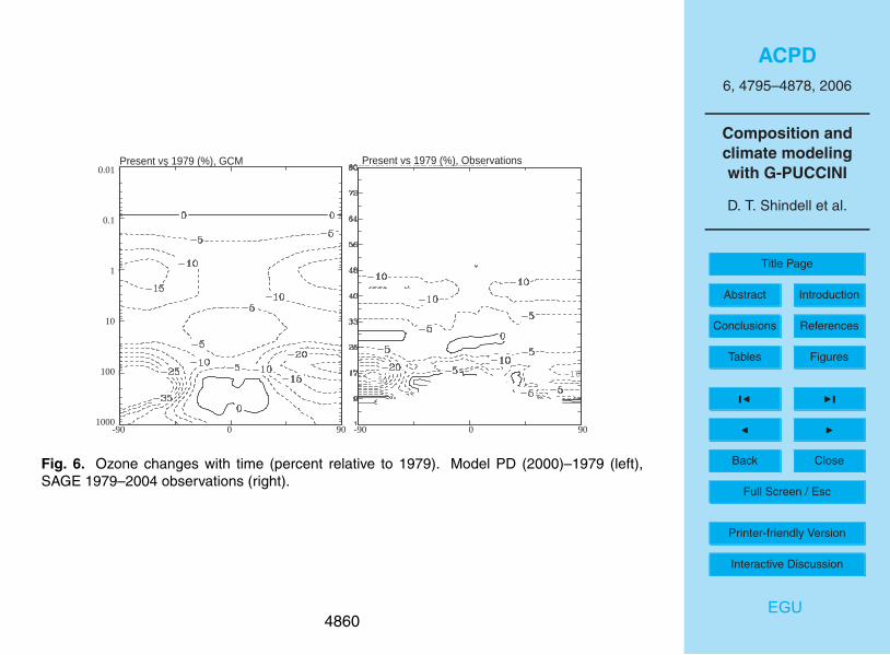
ACPD6, 4795–4878, 2006



Title Page



Tables Figures

J I

J I

Back Close

Full Screen / Esc



EGU

Present vs 1979 (%), GCM Present vs 1979 (%), Observations

-30-10

1000

100

10

1

0.1

0.01

-90 900 -90 900

Fig. 6. Ozone changes with time (percent relative to 1979). Model PD (2000)–1979 (left),SAGE 1979–2004 observations (right).

4860





ACPD6, 4795–4878, 2006



Title Page



Tables Figures

J I

J I

Back Close

Full Screen / Esc



EGU

1 2 3 4 5 6 7 8 9 10 11 12

200

400

600

800

1000

1200

1400

1600

1800Resolute, 125 hPa

Mon

th

1 2 3 4 5 6 7 8 9 10 11 12

100

250

400

550

700

850

1000

1150

Hohenpeissenberg, 125 hPa

Mon

th

1 2 3 4 5 6 7 8 9 10 11 12 0

50

100

150

200

250

300

350Hilo, 125hPa

Mon

th

1 2 3 4 5 6 7 8 9 10 11 12 0

100

200

300

400

500

600

700

800

900200 hPa

Mon

th

1 2 3 4 5 6 7 8 9 10 11 12 0

100

200

300

400

500

600200 hPa

Mon

th

1 2 3 4 5 6 7 8 9 10 11 12 0

25

50

75

100

125

150200 hPa

Mon

th

1 2 3 4 5 6 7 8 9 10 11 12 0

100

200

300

400300 hPa

Mon

th

1 2 3 4 5 6 7 8 9 10 11 12 0

50

100

150

200300 hPa

Mon

th

1 2 3 4 5 6 7 8 9 10 11 12 0

25

50

75

100

125

150300 hPa

Mon

th1 2 3 4 5 6 7 8 9 10 11 12

0

25

50

75

100

125

150500 hPa

Mon

th

1 2 3 4 5 6 7 8 9 10 11 12 0

25

50

75

100

125

150500 hPa

Mon

th

1 2 3 4 5 6 7 8 9 10 11 12 0

25

50

75

100

125

150500 hPa

Mon

th

1 2 3 4 5 6 7 8 9 10 11 12 0

25

50

75

100900 hPa

Ozone (ppbv)

Mon

th

1 2 3 4 5 6 7 8 9 10 11 12 0

25

50

75

100900 hPa

Ozone (ppbv)

Mon

th

1 2 3 4 5 6 7 8 9 10 11 12 0

25

50

75

100900 hPa

Ozone (ppbv)

Mon

th

Fig. 7. Comparison of ozone’s annual cycle in the model with an ozonesonde climatology(Logan, 1999) at the given locations and pressure levels. Solid lines give observed meanvalues, while filled circles and open triangles show results from the tropospheric chemistry-only and full chemistry simulations, respectively. Model values have been interpolated onto thegiven pressure levels.

4861





ACPD6, 4795–4878, 2006



Title Page



Tables Figures

J I

J I

Back Close

Full Screen / Esc



EGU

1 2 3 4 5 6 7 8 9 10 11 12 0

25

50

75

100

125

150

175

200Natal, 125 hPa

Mon

th

1 2 3 4 5 6 7 8 9 10 11 12 0

100

200

300

400

500

600

700

800Lauder, 125 hPa

Mon

th

1 2 3 4 5 6 7 8 9 10 11 12 100

200

300

400

500

600

700

800

900

1000Syowa, 125 hPa

Mon

th

1 2 3 4 5 6 7 8 9 10 11 12 0

50

100

150

200200 hPa

Mon

th

1 2 3 4 5 6 7 8 9 10 11 12 0

100

200

300

400

500200 hPa

Mon

th

1 2 3 4 5 6 7 8 9 10 11 12 0

100

200

300

400

500200 hPa

Mon

th

1 2 3 4 5 6 7 8 9 10 11 12 0

25

50

75

100

125

150300 hPa

Mon

th

1 2 3 4 5 6 7 8 9 10 11 12 0

25

50

75

100

125

150300 hPa

Mon

th

1 2 3 4 5 6 7 8 9 10 11 12 0

50

100

150

200300 hPa

Mon

th1 2 3 4 5 6 7 8 9 10 11 12

0

25

50

75

100500 hPa

Mon

th

1 2 3 4 5 6 7 8 9 10 11 12 0

25

50

75

100500 hPa

Mon

th

1 2 3 4 5 6 7 8 9 10 11 12 0

25

50

75

100500 hPa

Mon

th

1 2 3 4 5 6 7 8 9 10 11 12 0

10

20

30

40

50900 hPa

Ozone (ppbv)

Mon

th

1 2 3 4 5 6 7 8 9 10 11 12 0

10

20

30

40

50900 hPa

Ozone (ppbv)

Mon

th

1 2 3 4 5 6 7 8 9 10 11 12 0

10

20

30

40

50900 hPa

Ozone (ppbv)

Mon

th

Fig. 7. Continued.

4862





ACPD6, 4795–4878, 2006



Title Page



Tables Figures

J I

J I

Back Close

Full Screen / Esc



EGU

1 2 3 4 5 6 7 8 9 10 11 12 0

10

20

30

40

50

60Reykjavik (64N,22W)

Ozo

ne

(pp

bv)

1 2 3 4 5 6 7 8 9 10 11 12 0

10

20

30

40

50

60Hohenpeissenberg (48N,11E)

Ozo

ne

(pp

bv)

1 2 3 4 5 6 7 8 9 10 11 12 0

10

20

30

40

50

60

NYVTPAMA

PA NY VT MA

Ozo

ne

(pp

bv)

1 2 3 4 5 6 7 8 9 10 11 12 0

10

20

30

40

50

60Rockport IN (38N,87W)

Ozo

ne

(pp

bv)

1 2 3 4 5 6 7 8 9 10 11 12 0

10

20

30

40

50

60Bermuda (32N,64W)

Ozo

ne

(pp

bv)

1 2 3 4 5 6 7 8 9 10 11 12 0

10

20

30

40

50

60Venezuela (9N,63W)

Ozo

ne

(pp

bv)

1 2 3 4 5 6 7 8 9 10 11 12 0

10

20

30

40

50

60Brazzaville (4S,15E)

Month

Ozo

ne

(pp

bv)

1 2 3 4 5 6 7 8 9 10 11 12 0

10

20

30

40

50

60Cuiaba (16S,56W)

Month

Ozo

ne

(pp

bv)

1 2 3 4 5 6 7 8 9 10 11 12 0

10

20

30

40

50

60South Pole (90S,0E)

Month

Ozo

ne

(pp

bv)

Tropospheric chemistry-onlyObservationsFull chemsitry

Fig. 8. Annual cycles of surface ozone in the model and in observations. Solid lines give ob-served mean values, while filled circles and open triangles show results from the troposphericchemistry-only and full chemistry simulations, respectively. Note that observations at Brazzav-ille and Venezuela are averages of daily maximum values, so represent an upper bound.

4863





ACPD6, 4795–4878, 2006



Title Page



Tables Figures

J I

J I

Back Close

Full Screen / Esc



EGU

0 10 20 30 40 50 60 0

10

20

30

40

50

60

Observations (ppbv)

Mod

el (

ppbv

)r2=0.48

Fig. 9. Correlation diagram of observed and modeled annual average surface ozone at 40locations using the data of Logan (1999).

4864





ACPD6, 4795–4878, 2006



Title Page



Tables Figures

J I

J I

Back Close

Full Screen / Esc



EGU

0 200 400 600 800 1000

100

200

300

400

500

600

700

800

900

1000

Standard + dust chemobserved meanmaxmin

Standard runStandard - liquid tracers

Fiji (PEM Tropics B) MAR/APR

Pre

ssur

e (h

Pa)

0 200 400 600 800 1000

100

200

300

400

500

600

700

800

900

1000

Fiji (PEM Tropics A) SEP

0 200 400 600 800 1000

100

200

300

400

500

600

700

800

900

1000

Japan (PEM West B) FEB/MAR

Pre

ssur

e (h

Pa)

0 200 400 600 800 1000

100

200

300

400

500

600

700

800

900

1000

Philippine Sea (PEM West B) FEB/MAR

0 200 400 600 800 1000

100

200

300

400

500

600

700

800

900

1000

E-Brazil (TRACE A) OCT

HNO3 (pptv)

Pre

ssur

e (h

Pa)

0 200 400 600 800 1000

100

200

300

400

500

600

700

800

900

1000

S-Atlantic (TRACE A) OCT

HNO3 (pptv)

Fig. 10. Nitric acid profiles in observations and model simulations for the indicated locationsand seasons. Solid and dotted lines indicate measured mean values and standard deviations,respectively. Values from the model are show as lines with symbols, with solid triangles showingthe standard simulation, open squares showing the simulation with the liquid tracer budgetremoved, and filled circles showing the standard simulation but with heterogeneous chemistryon mineral dust included. Observations are from Emmons et al. (2000).

4865





ACPD6, 4795–4878, 2006



Title Page



Tables Figures

J I

J I

Back Close

Full Screen / Esc



EGU

Fig. 11. Observed and modeled seasonal lightning flash rates (flashes/km2/season). The leftcolumn shows observations from the Optical Transient Detector during 1995–1996 (other yearsare similar), while the right shows model results. The top row are June-August averages, whilethe bottom row are December-February averages. Note that there are no measurements athigh latitudes, and the scale used here is non-linear.

4866





ACPD6, 4795–4878, 2006



Title Page



Tables Figures

J I

J I

Back Close

Full Screen / Esc



EGU

1650

1700

1750

1800

1850

1900

1950

-90 -60 -30 0 30 60 90

Meth

ane (

ppbv)

Latitude

Fig. 12. Zonal mean surface methane in the NOAA GMD network (solid circles) for 2000–2004and in the model (solid line). Note that the model is a true zonal average while the observationsare averages over locations with observations.

4867





ACPD6, 4795–4878, 2006



Title Page



Tables Figures

J I

J I

Back Close

Full Screen / Esc



EGU

0 200 400 600 800 1000 1200 1400 0

200

400

600

800

1000

1200

1400

Observations (pptv)

Mod

el (

pptv

)r2=0.54

Fig. 13. Surface sulfate in observations and in the GCM simulations with coupled chemistryand aerosols. Observations are taken from the IMPROVE network (http://vista.cira.colostate.edu/improve), the EMEP network (http://www.emep.int), and J. M. Prospero and D. L. Savoie(unpublished data, 1999).

4868





http://vista.cira.colostate.edu/improve

http://vista.cira.colostate.edu/improve

http://www.emep.int

ACPD6, 4795–4878, 2006



Title Page



Tables Figures

J I

J I

Back Close

Full Screen / Esc



EGU

Present vs preindustrial

Temperature (C) Ozone (%)

1000

100

10

1

0.1

0.01

-90 900 -90 900

Fig. 14. Modeled differences between the present day and the preindustrial due to both emis-sions and climate changes in annual average zonal mean temperature (left, C) and ozone (right,% relative to PD). Note that plotting ozone changes relative to PD makes them comparable tothe results from the future simulations it can lead to very large values in regions where PDamounts are small.

4869





ACPD6, 4795–4878, 2006



Title Page



Tables Figures

J I

J I

Back Close

Full Screen / Esc



EGU

Change from PI to PD, climate and emissions

Change from PD to 2100, A2 climate only

Change from PD to 2100, A2 climate and emissions

Fig. 15. Changes in annual average surface ozone (ppbv) for the indicated climate or climateand emissions perturbations. Values in the upper right corner show the global mean change.Note change in scale between panels.

4870





ACPD6, 4795–4878, 2006



Title Page



Tables Figures

J I

J I

Back Close

Full Screen / Esc



EGU

ClO OH

H2O NO x

1000

100

10

1

0.1

0.01

1000

100

10

1

0.1

0.01

Present vs preindustrial

Fig. 16. Changes in water (tenths ppmv, top left), NOx (tens pptv, top right), ClO (tens pptv,bottom left) and OH (104 molecules/cm3 bottom right) between the present and the preindustrialin simulations forced by emissions and climate changes. Tropospheric changes in water havebeen blanked out for clarity.

4871





ACPD6, 4795–4878, 2006



Title Page



Tables Figures

J I

J I

Back Close

Full Screen / Esc



EGU

Future vs present, A2 emissions and climate

-90 900 -90 9001000

100

10

1

0.1

0.01Temperature (C) Ozone (%)

Fig. 17. Simulated changes between the 2100 A2 emissions and climate run and the present-day for annual average zonal mean temperature (left, C) and ozone (right, %).

4872





ACPD6, 4795–4878, 2006



Title Page



Tables Figures

J I

J I

Back Close

Full Screen / Esc



EGU

ClO OH

H2O NO x


1000

100

10

1

0.1

0.01

1000

100

10

1

0.1

0.01

-10 -20

Fig. 18. Changes in water (tenths ppmv, top left), NOx (tens pptv, top right), ClO (tens pptv,bottom left) and OH (104 molecules/cm3 bottom right) between the 2100 A2 emissions plusclimate run and the present-day simulation.

4873





ACPD6, 4795–4878, 2006



Title Page



Tables Figures

J I

J I

Back Close

Full Screen / Esc



EGU

Future vs present, A2 climate only


-90 900 -90 9001000

100

10

1

0.1

0.01

Fig. 19. Simulated changes between the 2100 A2 climate-only run and the present-day forannual average zonal mean temperature (left, C) and ozone (right, %).

4874





ACPD6, 4795–4878, 2006



Title Page



Tables Figures

J I

J I

Back Close

Full Screen / Esc



EGU

Future vs present, A2 climate only


Fig. 20. Differences in zonal mean ozone change (10 kg/s) due to dynamics (left column),moist convection (center column) and chemistry (right column) between the PD and the A2climate-only (top row) and A2 climate and emissions (bottom row) simulations.

4875





ACPD6, 4795–4878, 2006



Title Page



Tables Figures

J I

J I

Back Close

Full Screen / Esc



EGU

Future vs present, A1B emissions and climate


-90 900 -90 9001000

100

10

1

0.1

0.01

Fig. 21. Modeled future A1B 2100 emissions and climate change relative to the present-day inzonal mean annual average temperature (left, C) and ozone (right, %).

4876





ACPD6, 4795–4878, 2006



Title Page



Tables Figures

J I

J I

Back Close

Full Screen / Esc



EGU

ClO OH

H2O NO x

Future vs present, A1B emissions and climate

1000

100

10

1

0.1

0.01

1000

100

10

1

0.1

0.01

-20 -10

-20

-40

Fig. 22. Changes in water (tenths ppmv, top left), NOx (tens pptv, top right), ClO (tens pptv,bottom left) and OH (104 molecules/cm3 bottom right) between the 2100 A1B composition plusclimate run and the present-day simulation.

4877





ACPD6, 4795–4878, 2006



Title Page



Tables Figures

J I

J I

Back Close

Full Screen / Esc



EGU

Future vs present, A1B emissions only


-90 900 -90 9001000

100

10

1

0.1

0.01

Fig. 23. Impact of A1B composition change (Future vs PD) on annual average zonal meantemperature (left, C) and ozone (right, %).

4878





simulations of preindustrial, present-day, and 2100 conditions in … · 20 interactions important...

Documents