Simulation with System Dynamics Models

IE 680 Spring 2007

Po-Ching C. DeLaurentis

April 19, 2007

Outline Systems Thinking System Dynamics (SD) Paradigm Comparison Basics of System Dynamics Quantification Challenges Simulation with System Dynamics- An Example Summary System Dynamics Resources

Systems Thinking

Systems Thinking Early 20th century physicists began to

challenge Newtonian precepts; Werner Heisenberg, Norbert Weiner, Von Bertalanffy

“An approach for developing models to promote our understanding of events, patterns of behavior resulting in the events, and even more importantly, the underlying structure responsible for the patterns of behavior”*

* http://www.systems-thinking.org

System Dynamics

System Dynamics Introduced by Jay Forrester of MIT in 1958

“The study of information-feedback characteristics of industry activity to show how organizational structure, amplification (in policies), and time delays (in decisions and actions) interact to influence the success of the enterprise” (Forrest 1958 & 1961)

Paradigm Comparison of System Dynamics, Discrete Event & Agent Based

Borshchev A , Filippov A. From System Dynamics and Discrete Event to Practical Agent Based Modeling: Reasons, Techniques, Tools. Proceedings of the 22nd International Conference, July 25-29, 2004, Oxford, England, UK.

High Abstraction Less Details Macro Level

Strategic Level

Middle Abstraction Medium Details

Meso Level Tactical Level

Low Abstraction More Details

Micro Level Operational Level Individual objects, exact sizes, distances, velocities, timings, …

Agent Based Active objects

Individual behavior rules

Direct or indirect interaction

Environment models

Discrete Event Entities (passive

objects)

Flowcharts and/or transport networks

Resources

Aggregates, Global Casual Dependencies, Feedback Dynamics, …

Mainly discrete

System Dynamics Levels (aggregates)

Stock-and-Flow Diagrams

Feedback loops

Mainly continuous

Basics of System Dynamics

Stock A Stock B

Rate

Decision Rules

Stock-and-Flow

Casual Loops

Basics of System Dynamics (cont’d)

Brownies_in_Stomach(t) = Brownies_in_Stomach (t - dt) + (eating - digesting) * dt

INIT Brownies_in_Stomach = 0

DOCUMENT: Initially Andy’s stomach is empty.

UNITS: brownies

eating = 1

DOCUMENT: Andy eats a brownie every hour.

UNITS: brownies/hour

digesting = 1/2

DOCUMENT: Andy digests 1 brownie every 2 hours. He therefore digests a half a brownie every hour.

UNITS: brownies/hour

Basics of System Dynamics (cont’d)

Wide Range of System Dynamics Applications Corporate planning and policy design Economic behavior Public management and policy Biological and medical modeling Energy and the environment Supply chain management

Quantification ChallengesQuantification Challenges

Quantification Challenges System dynamics is strategic in orientation and it

is often seen to have ‘soft’ variables

Example (Coyle 2000): Consumer Satisfaction as an influence on

New_Order_Inflow_Rate = Basic_Inflow * Satisfaction_Multiplier

A variable that may range from 0 to an upper limit, and have a nonlinear relationship with Consumer Satisfaction

Quantification Challenges (Cont’d) If it becomesNew_Order_Inflow_Rate = Basic_Inflow * Satisfaction_Multiplier * Quality_Multiplier * Price_Multimplier * etc.

The number of uncertainties becomes very large;

Strong assumption that multipliers are multiplicative.

EX: 0.5 * 0.5 * 0.5 = 0.125 only 25% of 0.5

0.510 = 0.000977 only 1/500 of 0.5

Quantification Challenges- Example

Simulation Example

Police & Driver– A System Dynamics Model for a Mixed Strategy Game (Kim & Kim, 1997) System dynamics: dynamic fluctuations of a system Game Theory

Players; preferences & strategies; payoff/utility functions Players change decisions in response to other players’

actions Finding equilibrium states in game situation Dominant vs. mixed strategies

Police & Driver Game “You are driving your car in a hurry…there are two states

of the world: either the police are nearby or they are not. There are two actions to choose from: either to violate the speed limit or to abide by the law.” (Tsebelis 1989)

Police

Patrol Not Patrol

DriverSpeed a1, a2 b1, b2

Not Speed c1, c2 d1, d2

Note: c1 > a1 b1 > d1

a2 > b2d2 > c2

p

1-p

q 1-q

Police & Driver Game (Cont’d) Mixed strategy equilibrium results:

p = prob. with which the driver chooses to speed q = prob. with which the policeman decides to patrol Solved for:

p* = (d2-c2)/(a2-b2+d2-c2)q* = (b1-d1)/(b1-d1+c1-a1)

Observation The probability of the driver’s law violation is not

determined by the payoffs for the driver Increase in penalty ( a1)

Argument A contradiction to common sense: increase in penalty is

conceived as one the most effective tools for policy implementation

Police & Driver Game with System Dynamics

Why does game theory produce theorems inconsistent with common sense? Game theory applicability Equilibrium applicability

How to model this game with SD? Probability of players’ behaviors

Two independent players in the game Population mixed-strategy game

System Dynamics Diagram of the Game

parameters

Policemen in Office

Policemen in Patrolling

Drivers in Violation

Drivers in Conforming

Patrol to office

Quit Patrol

Go Patrol

Office to Patrol

Patrolling Time

Quitting Time

Difference eup eunp

euno

ppcnpppvnp

eupppvp

ppcp

prob v

Speed Down Time

Speed Down

Speed Up

Conform to ViolationSpeed Up

Time

Violation to Conform

Difference euv eunv

dpcnp

dpcp

eunv

prob p

euv

dpvp

dpvnp

System Dynamics Diagram of the Game (redrawn)

parameters

Simulation Results Oscillation Rather than Equilibrium

Tendency towards the equilibrium state

But it takes a long time!!

p*=0.25 (2:prob p)

q* = 0.5 (1:prob v)

Simulation Results (Cont’d) The Effectiveness of Penalty Increase

Increase in Penalty

p*=0.25 (2:prob p)

q* = 0.22 (1:prob v)

Tendency towards the equilibrium state

Prob. of violation reduced to < 0.25 for about 50 days

Simulation Results (Cont’d) Considering Information Delay Between the Police & the Driver

Larger amplitude

Not approaching steady state

10 days for Driver

5 days for Police

Simulation Results (Cont’d) The Effectiveness of Penalty Increase with Information Delay

Increase in Penalty

Prob. of violation is lightly reduced

Simulation Results (Cont’d) Effectiveness of Automatic Penalty Management (without info

delay) Police change the amount of penalty in line with probability of changes

in law violation

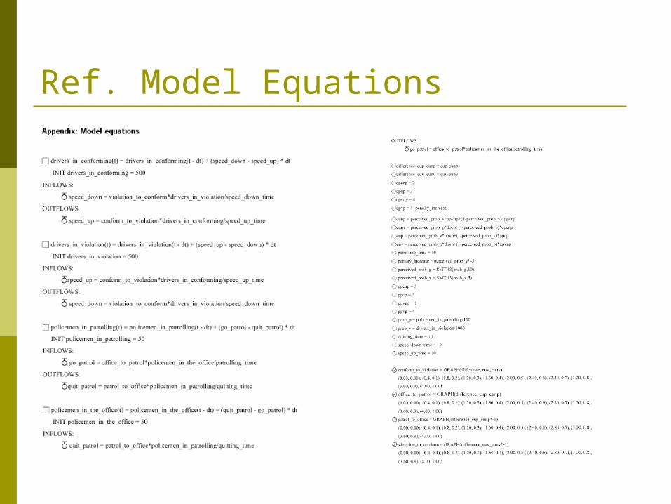
Equations

Equilibrium reached after a short period of fluctuation

Policy Implications

Simulation results suggest: Temporarily reduce the violation tendency of drivers by

changing the amount of penalty Penalty management can decrease the amplitude of

fluctuating behavior of drivers For policy makers

Temporary reductions of speed limit violation will be a sufficient incentive for introduction of penalty increase

Penalty management can reduce the amplitude of fluctuation violations

Max. level of violation probability of car accidents?

Insights

Information delay & policy interruptions exist in a dynamic system

Mixed-strategy equilibrium may be a poor guide Equilibrium vs. Steady State In the real world, players are usually myopic

System Dynamics: simulate evolutionary processes toward (non-)equilibrium states

Game Theory: a framework for modeling the world of competition and cooperation

Summary System Dynamics

Stock-and-flow Casual loops Higher, strategic level modeling Dynamic behaviors of a system Transient processes Challenges: quantification of influencing

factors; underlying effects

System Dynamics Resources

System Dynamics Society http://www.systemdynamics.org/

Sterman, Business Dynamics: Systems Thinking and Modeling for a Complex World, McGraw-Hill/Irwin, 2000

Software VenSim– http://www.vensim.com/ Stella– http://www.iseesystems.com/

Questions

Ref. Model Equations

System Dynamics Diagram of the Game (Cont’d)

Parameters