simulation techniques for cosmological simulations

Space Sci Rev (2008) 134: 229–268DOI 10.1007/s11214-008-9316-5

Simulation Techniques for Cosmological Simulations

K. Dolag · S. Borgani · S. Schindler · A. Diaferio ·A.M. Bykov

Received: 13 November 2007 / Accepted: 14 December 2007 / Published online: 15 February 2008© Springer Science+Business Media B.V. 2008

Abstract Modern cosmological observations allow us to study in great detail the evolu-tion and history of the large scale structure hierarchy. The fundamental problem of accurateconstraints on the cosmological parameters, within a given cosmological model, requiresprecise modelling of the observed structure. In this paper we briefly review the current mosteffective techniques of large scale structure simulations, emphasising both their advantagesand shortcomings. Starting with basics of the direct N -body simulations appropriate to mod-elling cold dark matter evolution, we then discuss the direct-sum technique GRAPE, particle-mesh (PM) and hybrid methods, combining the PM and the tree algorithms. Simulations ofbaryonic matter in the Universe often use hydrodynamic codes based on both particle meth-ods that discretise mass, and grid-based methods. We briefly describe Eulerian grid methods,and also some variants of Lagrangian smoothed particle hydrodynamics (SPH) methods.

K. Dolag (�)Max-Planck-Institut für Astrophysik, P.O. Box 1317, 85741 Garching, Germanye-mail: [email protected]

S. BorganiDepartment of Astronomy, University of Trieste, via Tiepolo 11, 34143 Trieste, Italye-mail: [email protected]

S. SchindlerInstitut für Astro- und Teilchenphysik, Universität Innsbruck, Technikerstr. 25, 6020 Innsbruck, Austriae-mail: [email protected]

A. DiaferioDipartimento di Fisica Generale “Amedeo Avogadro”, Università degli Studi di Torino, Turin, Italye-mail: [email protected]

A. DiaferioIstituto Nazionale di Fisica Nucleare (INFN), Sezione di Torino, via P. Giuria 1, 10125 Turin, Italy

A.M. BykovA.F. Ioffe Institute of Physics and Technology, 194021 St. Petersburg, Russiae-mail: [email protected]

230 K. Dolag et al.

Keywords Cosmology: theory · Large-scale structure of universe · Hydrodynamics ·Method: numerical, N -body simulations

1 Introduction

In the hierarchical picture of structure formation, small objects collapse first and then mergeto form larger and larger structures in a complex manner. This formation process reflects onthe intricate structure of galaxy clusters, whose properties depend on how the thousands ofsmaller objects that the cluster accretes are destroyed or survive within the cluster gravita-tional potential. These merging events are the source of shocks, turbulence and accelerationof relativistic particles in the intracluster medium, which, in turn, lead to a redistribution oramplification of magnetic fields, and to the acceleration of cosmic rays. In order to modelthese processes realistically, we need to resort to numerical simulations which are capa-ble of resolving and following correctly the highly non-linear dynamics. In this paper, webriefly describe the methods which are commonly used to simulate galaxy clusters within acosmological context.

Usually, choosing the simulation setup is a compromise between the size of the regionthat one has to simulate to fairly represent the object(s) of interest, and the resolution neededto resolve the objects at the required level of detail. Typical sizes of the simulated volume area megaparsec scale for an individual galaxy, tens to hundreds of megaparsecs for a galaxypopulation, and several hundreds of megaparsecs for a galaxy cluster population. The massresolution varies from ≈ 105 M� up to ≈ 1010 M�, depending on the object studied, while,nowadays, one can typically reach the resolution of a few hundred parsec for individualgalaxies and above the kiloparsec scale for cosmological boxes.

2 N -Body (Pure Gravity)

Over most of the cosmic time of interest for structure formation, the Universe is dominatedby dark matter. The most favourable model turned out to be the so-called cold dark matter(CDM) model. The CDM can be described as a collisionless, non-relativistic fluid of parti-cles of mass m, position x and momentum p. In an expanding background Universe (usuallydescribed by a Friedmann-Lemaître model), with a = (1 + z)−1 being the Universe scalefactor, x is the comoving position and the phase-space distribution function f (x,p, t) of thedark-matter fluid can be described by the collisionless Boltzmann (or Vlasov) equation

∂f

∂t+ p

ma2∇f − m∇�

∂f

∂p= 0 (1)

coupled with the Poisson equation

∇2�(x, t) = 4πGa2 [ρ(x, t) − ρ(t)] , (2)

where � is the gravitational potential and ρ(t) is the background density. The proper massdensity

ρ(x, t) =∫

f (x,p, t)d3p (3)

can be inferred by integrating the distribution function over the momenta p = ma2x.

Simulation Techniques for Cosmological Simulations 231

This set of equations represents a high-dimensional problem. It is therefore usuallysolved by sampling the phase-space density by a finite number N of tracer particles. Thesolution can be found through the equation of motion of the particles (in comoving coordi-nates),

dpdt

= −m∇� (4)

and

dxdt

= pma2

. (5)

Introducing the proper peculiar velocity v = ax these equations can be written as

dvdt

+ va

a= −∇�

a. (6)

The time derivative of the expansion parameter, a, can be obtained from the Friedmannequation

a = H0

√1 + �0(a−1 − 1) + ��(a2 − 1), (7)

where we have assumed the dark energy to be equivalent to a cosmological constant. For amore detailed description of the underlying cosmology and related issues, see for examplePeebles (1980) or others.

There are different approaches: to solve directly the motion of the tracer particles, or tosolve the Poisson equation. Some of the most common methods will be described briefly inthe following sections.

2.1 Direct Sum (GRAPE, GPU)

The most direct way to solve the N -body problem is to sum directly the contributions of allthe individual particles to the gravitational potential

�(r) = −G∑

j

mj

(|r − rj |2 + ε2)12

. (8)

In principle, this sum would represent the exact (Newtonian) potential which generates theparticles’ acceleration. As mentioned before, the particles do not represent individual darkmatter particles, but should be considered as Monte Carlo realisations of the mass distri-bution, and therefore only collective, statistical properties can be considered. In such sim-ulations, close encounters between individual particles are irrelevant to the physical prob-lem under consideration, and the gravitational force between two particles is smoothed byintroducing the gravitational softening ε. This softening reduces the spurious two-body re-laxation which occurs when the number of particles in the simulation is not large enoughto represent correctly a collisionless fluid. This situation however is unavoidable, becausethe number of dark matter particles in real systems is orders of magnitude larger than thenumber that can be handled in a numerical simulation. Typically, ε is chosen to be 1/20–1/50 of the mean inter-particle separation within the simulation. In general, this direct-sumapproach is considered to be the most accurate technique, and is used for problems wheresuperior precision is needed. However this method has the disadvantage of being alreadyquite CPU intensive for even a moderate number of particles, because the computing timeis ∝ N2, where N is the total number of particles.

232 K. Dolag et al.

Rather than searching for other software solutions, an alternative approach to solve theN2-bottleneck of the direct-sum technique is the GRAPE (GRAvity PipE) special-purposehardware (see e.g. Ito et al. 1993 and related articles). This hardware is based on customchips that compute the gravitational force with a hardwired Plummer force law (8). Thishardware device thus solves the gravitational N -body problem with a direct summationapproach at a computational speed which is considerably higher than that of traditionalprocessors.

For the force computation, the particle coordinates are first loaded onto the GRAPEboard, then the forces for several positions (depending on the number of individual GRAPEchips installed in the system) are computed in parallel. In practise, there are some technicalcomplications when using the GRAPE system. One is that the hardware works internallywith special fixed-point formats or with limited floating point precision (depending on theversion of the GRAPE chips used) for positions, accelerations and masses. This results ina reduced dynamic range compared to the standard IEEE floating point arithmetic. Further-more, the communication time between the host computer and the GRAPE system can bean issue in certain circumstances. However, newer versions of the GRAPE chips circumventthis problem, and can also be combined with the tree algorithms (which are described indetail in the next section), see Fukushige et al. (1991), Makino (1991), Athanassoula et al.(1998), Kawai et al. (2000).

By contrast, the graphic processing unit (GPU) on modern graphic cards now providesan alternative tool for high-performance computing. The original purpose of the GPU isto serve as a graphics accelerator for speeding up the image processing, thereby allowingone to perform simple instructions on multiple data. It has therefore become an active areaof research to use the GPUs of the individual members of computer clusters. Althoughvery specialised, many of those computational algorithms are also needed in computationalastrophysics, and therefore the GPU can provide significantly more computing power thanthe host system; thereby providing a high performance with typically large memory sizeand at relatively low cost, which represents a valid alternative to special purpose hardwarelike GRAPE. For recent applications to astrophysical problems see Schive et al. (2007) andreferences therein.

2.2 Tree

The primary method of solving the N -body problem is a hierarchical multipole expansion,commonly called a tree algorithm. This method groups distant particles into larger cells,allowing their gravity to be accounted for by means of a single multipole force. Instead ofrequiring N − 1 partial force evaluations per particle, as needed in a direct-summation ap-proach, the gravitational force on a single particle can be computed with substantially feweroperations, because distant groups are treated as “macro” particles in the sum. In this mannerthe sum usually reduces to N log(N) operations. Note however that this scaling is only truefor homogeneous particle distributions, whereas the scaling for strongly inhomogeneousdistributions, as present in evolved cosmological structures, can be less efficient.

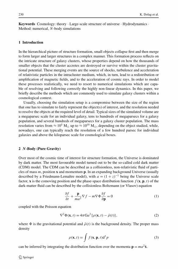
In practise, the hierarchical grouping that forms the basis of the multipole expansion ismost commonly obtained by a recursive subdivision of space. In the approach of Barnes andHut (1986), a cubical root node is used to encompass the full mass distribution; the cubeis repeatedly subdivided into eight daughter nodes of half the side-length each, until oneends up with ‘leaf’ nodes containing single particles (see Fig. 1). Forces are then obtainedby “walking” the tree. In other words, starting at the root node, a decision is made as towhether or not the multipole expansion of the node provides an accurate enough partial


Fig. 1 Schematic illustration of the Barnes and Hut (1986) oct-tree in two dimensions. The particles are firstenclosed in a square (root node). This square is then iteratively subdivided into four squares of half the size,until exactly one particle is left in each final square (leaves of the tree). In the resulting tree structure, eachsquare can be the progenitor of up to four siblings. Taken from Springel et al. (2001b)

force. If the answer is ‘yes’, the multipole force is used and the walk along this branch ofthe tree can be terminated; if the answer is ‘no’, the node is “opened”, i.e. its daughter nodesare considered in turn. Clearly, the multipole expansion is in general appropriate for nodesthat are sufficiently small and distant. Most commonly one uses a fixed angle (typically≈ 0.5 rad) as opening criteria.

It should be noted that the final result of the tree algorithm will in general only repre-sent an approximation to the true force. However, the error can be controlled convenientlyby modifying the opening criterion for tree nodes, because a higher accuracy is obtainedby walking the tree to lower levels. Provided that sufficient computational resources are in-vested, the tree force can then be made arbitrarily close to the well-specified correct force.Nevertheless evaluating the gravitational force via a tree leads to an inherent asymmetryin the interaction between two particles. It is worth mentioning that there are extensionsto the standard tree, the so-called fast multipole methods, which avoid these asymmetries,and therefore have better conservation of momentum. For an N -body application of such atechnique see Dehnen (2000) and references therein. However, these methods compute theforces for all the particles at every time step and can not take advantage of using individualtime steps for different particles.

2.3 Particle-Mesh Methods

The Particle-Mesh (PM) method treats the force as a field quantity by computing it on amesh. Differential operators, such as the Laplacian, are replaced by finite difference approx-imations. Potentials and forces at particle positions are obtained by interpolation on the arrayof mesh-defined values. Typically, such an algorithm is performed in three steps. First, thedensity on the mesh points is computed by assigning densities to the mesh from the parti-cle positions. Second, the density field is transformed to Fourier space, where the Poissonequation is solved, and the potential is obtained using Green’s method. Alternatively, the po-tential can be determined by solving Poisson’s equation iteratively with relaxation methods.In a third step the forces for the individual particles are obtained by interpolating the deriv-atives of the potentials to the particle positions. Typically, the amount of mesh cells N usedcorresponds to the number of particles in the simulation, so that when structures form, onecan have large numbers of particles within individual mesh cells, which immediately illus-trates the shortcoming of this method; namely its limited resolution. On the other hand, thecalculation of the Fourier transform via a Fast Fourier Transform (FFT) is extremely fast, as

234 K. Dolag et al.

it only needs of order N logN operations, which is the advantage of this method. Note thathere N denotes the number of mesh cells. In this approach the computational costs do notdepend on the details of the particle distribution. Also this method can not take advantage ofindividual time steps, as the forces are always calculated for all particles at every time step.

There are many schemes to assign the mass density to the mesh. The simplest method isthe “Nearest-Grid-Point” (NGP). Here, each particle is assigned to the closest mesh point,and the density at each mesh point is the total mass assigned to the point divided by the cellvolume. However, this method is rarely used. One of its drawbacks is that it gives forcesthat are discontinuous. The “Cloud-in-a-Cell” (CIC) scheme is a better approximation tothe force: it distributes every particle over the nearest 8 grid cells, and then weighs themby the overlapping volume, which is obtained by assuming the particle to have a cubicshape of the same volume as the mesh cells. The CIC method gives continuous forces, butdiscontinuous first derivatives of the forces. A more accurate scheme is the “Triangular-Shaped-Cloud” (TSC) method. This scheme has an assignment interpolation function thatis piecewise quadratic. In three dimensions it employs 27 mesh points (see Hockney andEastwood 1988).

In general, one can define the assignment of the density ρm on a grid xm with spacing δ

from the distribution of particles with masses mi and positions xi , by smoothing the particlesover n times the grid spacing (h = nδ). Therefore, having defined a weighting function

W(xm − xi ) =∫

W

(x − xm

h

)S(x − xi , h)dx, (9)

where W (x) is 1 for |x| < 0.5 and 0 otherwise, the density ρm on the grid can be written as

ρm = 1

h3

∑i

miW(xi − xm). (10)

The shape function S(x, h) then defines the different schemes. The aforementioned NGP,CIC and TSC schemes are equivalent to the choice of 1, 2 or 3 for n and the Dirac δ func-tion δ(x), W (x/h) and 1 − |x/h| for the shape function S(x, h), respectively.

In real space, the gravitational potential � can be written as the convolution of the massdensity with a suitable Green’s function g(x):

�(x) =∫

g(x − x′)ρ(x′)dx′. (11)

For vacuum boundary conditions, for example, the gravitational potential is

�(x) = −G∫

ρ(x′)|x − x′|dx′, (12)

with G being the gravitational constant. Therefore the Green’s function, g(x) =−G/|x|, represents the solution of the Poisson equation ∇2�(x) = 4πGρ(x), recalling that∇2

x (|x − x′|)−1 = 4πδ(x − x′). By applying the divergence theorem to the integral form ofthe above equation, it is then easy to see that, in spherical coordinates,

∫V

∇2

(1

r

)dV =

∫S

∇(

1

r

)dS =

∫ 2π

0

∫ π

0

∂

∂r

(1

r

)r2sin(θ)dθdφ = −4π. (13)

Periodic boundary conditions are usually used to simulate an “infinite universe”, howeverzero padding can be applied to deal with vacuum boundary conditions.


In the PM method, the solution to the Poisson equation is easily found in Fourier space,where (11) becomes a simple multiplication

�(k) = g(k) ρ(k). (14)

Note that g(k) has only to be computed once, at the beginning of the simulation.After the calculation of the potential via Fast Fourier Transform (FFT) methods, the force

field f(x) at the position of the mesh points can be obtained by differentiating the potential,f(x) = ∇�(x). This can be done by a finite-difference representation of the gradient. In asecond order scheme, the derivative with respect to the x coordinate at the mesh positionsm = (i, j, k) can be written as

f(x)i,j,k = −�i+1,j,k − �i−1,j,k

2h. (15)

A fourth order scheme for the derivative would be written as

f(x)i,j,k = −4

3

�i+1,j,k − �i−1,j,k

2h+ 1

3

�i+2,j,k − �i−2,j,k

4h. (16)

Finally, the forces have to be interpolated back to the particle positions as

f(xi ) =∑m

W(xi − xm)fm, (17)

where it is recommended to use the same weighting scheme as for the density assignment;this ensures pairwise force symmetry between particles and momentum conservation.

The advantage of such PM methods is the speed, because the number of operations scaleswith N +Nglog(Ng), where N is the number of particles and Ng the number of mesh points.However, the disadvantage is that the dynamical range is limited by Ng , which is usually lim-ited by the available memory. Therefore, particularly for cosmological simulations, adaptivemethods are needed to increase the dynamical range and follow the formation of individualobjects.

In the Adaptive Mesh Refinement (AMR) techniques, the Poisson equation on the re-finement meshes can be treated as a Dirichlet boundary problem for which the boundaryvalues are obtained by interpolating the gravitational potential from the parent grid. In suchalgorithms, the boundaries of the refinement meshes can have an arbitrary shape; this fea-ture narrows the range of solvers that one can use for partial differential equation (PDEs).The Poisson equation on these meshes can be solved using the relaxation method (Hockneyand Eastwood 1988; Press et al. 1992), which is relatively fast and efficient in dealing withcomplicated boundaries. In this method the Poisson equation

∇2� = ρ (18)

is rewritten in the form of a diffusion equation,

∂�

∂τ= ∇2� − ρ. (19)

The point of the method is that an initial solution guess � relaxes to an equilibrium solution(i.e., solution of the Poisson equation) as τ → ∞. The finite-difference form of (2) is:

�n+1i,j,k = �n

i,j,k + τ

2

(6∑

nb=1

�nnb − 6�n

i,j,k

)− ρi,j,k τ, (20)

236 K. Dolag et al.

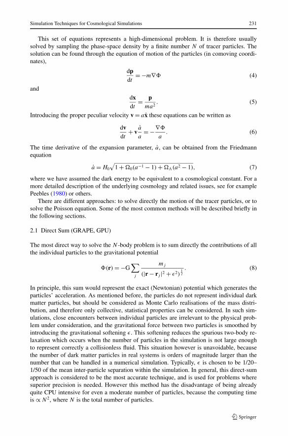
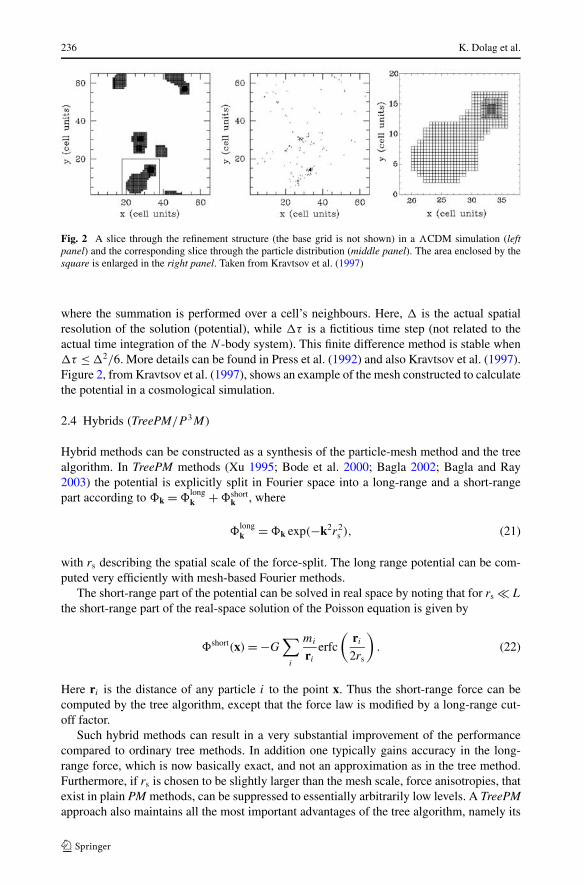
Fig. 2 A slice through the refinement structure (the base grid is not shown) in a �CDM simulation (leftpanel) and the corresponding slice through the particle distribution (middle panel). The area enclosed by thesquare is enlarged in the right panel. Taken from Kravtsov et al. (1997)

where the summation is performed over a cell’s neighbours. Here, is the actual spatialresolution of the solution (potential), while τ is a fictitious time step (not related to theactual time integration of the N -body system). This finite difference method is stable when τ ≤ 2/6. More details can be found in Press et al. (1992) and also Kravtsov et al. (1997).Figure 2, from Kravtsov et al. (1997), shows an example of the mesh constructed to calculatethe potential in a cosmological simulation.

2.4 Hybrids (TreePM/P 3M)

Hybrid methods can be constructed as a synthesis of the particle-mesh method and the treealgorithm. In TreePM methods (Xu 1995; Bode et al. 2000; Bagla 2002; Bagla and Ray2003) the potential is explicitly split in Fourier space into a long-range and a short-rangepart according to �k = �

longk + �short

k , where

�longk = �k exp(−k2r2

s ), (21)

with rs describing the spatial scale of the force-split. The long range potential can be com-puted very efficiently with mesh-based Fourier methods.

The short-range part of the potential can be solved in real space by noting that for rs L

the short-range part of the real-space solution of the Poisson equation is given by

�short(x) = −G∑

i

mi

ri

erfc

(ri

2rs

). (22)

Here ri is the distance of any particle i to the point x. Thus the short-range force can becomputed by the tree algorithm, except that the force law is modified by a long-range cut-off factor.

Such hybrid methods can result in a very substantial improvement of the performancecompared to ordinary tree methods. In addition one typically gains accuracy in the long-range force, which is now basically exact, and not an approximation as in the tree method.Furthermore, if rs is chosen to be slightly larger than the mesh scale, force anisotropies, thatexist in plain PM methods, can be suppressed to essentially arbitrarily low levels. A TreePMapproach also maintains all the most important advantages of the tree algorithm, namely its


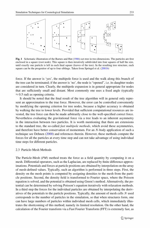
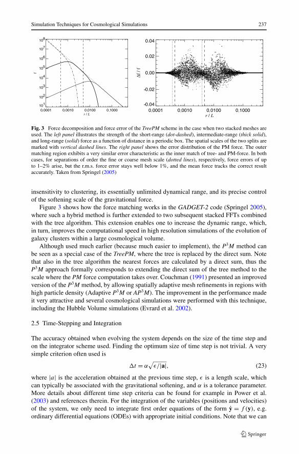
Fig. 3 Force decomposition and force error of the TreePM scheme in the case when two stacked meshes areused. The left panel illustrates the strength of the short-range (dot-dashed), intermediate-range (thick solid),and long-range (solid) force as a function of distance in a periodic box. The spatial scales of the two splits aremarked with vertical dashed lines. The right panel shows the error distribution of the PM force. The outermatching region exhibits a very similar error characteristic as the inner match of tree- and PM-force. In bothcases, for separations of order the fine or coarse mesh scale (dotted lines), respectively, force errors of upto 1–2% arise, but the r.m.s. force error stays well below 1%, and the mean force tracks the correct resultaccurately. Taken from Springel (2005)

insensitivity to clustering, its essentially unlimited dynamical range, and its precise controlof the softening scale of the gravitational force.

Figure 3 shows how the force matching works in the GADGET-2 code (Springel 2005),where such a hybrid method is further extended to two subsequent stacked FFTs combinedwith the tree algorithm. This extension enables one to increase the dynamic range, which,in turn, improves the computational speed in high resolution simulations of the evolution ofgalaxy clusters within a large cosmological volume.

Although used much earlier (because much easier to implement), the P3M method canbe seen as a special case of the TreePM, where the tree is replaced by the direct sum. Notethat also in the tree algorithm the nearest forces are calculated by a direct sum, thus theP3M approach formally corresponds to extending the direct sum of the tree method to thescale where the PM force computation takes over. Couchman (1991) presented an improvedversion of the P3M method, by allowing spatially adaptive mesh refinements in regions withhigh particle density (Adaptive P3M or AP3M). The improvement in the performance madeit very attractive and several cosmological simulations were performed with this technique,including the Hubble Volume simulations (Evrard et al. 2002).

2.5 Time-Stepping and Integration

The accuracy obtained when evolving the system depends on the size of the time step andon the integrator scheme used. Finding the optimum size of time step is not trivial. A verysimple criterion often used is

t = α√

ε/|a|, (23)

where |a| is the acceleration obtained at the previous time step, ε is a length scale, whichcan typically be associated with the gravitational softening, and α is a tolerance parameter.More details about different time step criteria can be found for example in Power et al.(2003) and references therein. For the integration of the variables (positions and velocities)of the system, we only need to integrate first order equations of the form y = f (y), e.g.ordinary differential equations (ODEs) with appropriate initial conditions. Note that we can

238 K. Dolag et al.

first solve this ODE for the velocity v and then treat x = v as an independent ODE, atbasically no extra cost.

One can distinguish implicit and explicit methods for propagating the system from step n

to step n+1. Implicit methods usually have better properties, however they need to solve thesystem iteratively, which usually requires inverting a matrix which is only sparsely sampled,and has the dimension of the total number of the data points, namely grid or particle points.Therefore, N -body simulations mostly adopt explicit methods.

The simplest (but never used) method to perform the integration of an ODE is calledEuler’s method; here the integration is just done by multiplying the derivatives with thelength of the time step. The explicit form of such a method can be written as

yn+1 = yn + f(yn) t, (24)

whereas the implicit version is written as

yn+1 = yn + f(yn+1) t. (25)

Note that in the latter equation yn+1 appears on the left and right side, which makes it clearwhy it is called implicit. Obviously the drawback of the explicit method is that it assumesthat the derivatives (e.g. the forces) do not change during the time step.

An improvement to this method can be obtained by using the mean derivative during thetime step, which can be written with the implicit mid-point rule as

yn+1 = yn + f[0.5(yn + yn+1)] t. (26)

An explicit rule using the forces at the next time step is the so-called predictor-correctormethod, where one first predicts the variables for the next time step

y0n+1 = yn + f(yn) t (27)

and then uses the forces calculated there to correct this prediction (the so-called correctorstep) as

yn+1 = yn + 0.5[f(yn) + f(y0n+1)] t. (28)

This method is accurate to second order.In fact, all these methods are special cases of the so-called Runge-Kutta method (RK),

which achieves the accuracy of a Taylor series approach without requiring the calculation ofhigher order derivatives. The price one has to pay is that the derivatives (e.g. forces) have tobe calculated at several points, effectively splitting the interval t into special subsets. Forexample, a second order RK scheme can be constructed by

k1 = f(yn) (29)

k2 = f(yn + k1 t) (30)

yn+1 = yn + 0.5(k1 + k2) t. (31)

In a fourth order RK scheme, the time interval t also has to be subsampled to calculate themid-points, e.g.

k1 = f(yn, tn) (32)


k2 = f(yn + k1 t/2, tn + t/2) (33)

k3 = f(yn + k2 t/2, tn + t/2) (34)

k4 = f(yn + k3 t/2, tn + t) (35)

yn+1 = yn +(

k1

6+ k2

3+ k3

3+ k4

6

) t. (36)

More details on how to construct the coefficient for an n-th order RK scheme are given ine.g. Chapra and Canale (1997).

Another possibility is to use the so-called leap-frog method, where the derivatives (e.g.forces) and the positions are shifted in time by half a time step. This feature can be used tointegrate directly the second order ODE of the form x = f(x). Depending on whether onestarts with a drift (D) of the system by half a time step or one uses the forces at the actualtime to propagate the system (kick, K), one obtains a KDK version

vn+1/2 = vn + f(xn) t/2 (37)

xn+1 = xn + vn+1/2 t (38)

vn+1 = vn+1/2 + f(xn+1) t/2 (39)

or a DKD version of the method

xn+1/2 = xn + vn t/2 (40)

vn+1 = vn + f(xn+1/2) t (41)

xn+1 = xn+1/2 + vn+1 t/2. (42)

This method is accurate to second order, and, as will be shown in the next paragraph, alsohas other advantages. For more details see Springel (2005).

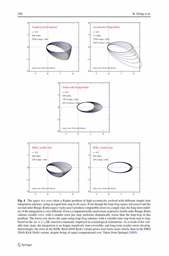
It is also clear that, depending on the application, a lower order scheme applied withmore, and thus smaller, time steps can be more efficient than a higher order scheme, whichenables the use of larger time steps. In the upper rows of Fig. 4, we show the numeri-cal integration of a Kepler problem (i.e. two point-like masses with large mass differencewhich orbit around each other like a planet-sun system) of high eccentricity e = 0.9, us-ing second-order accurate leap-frog and Runge-Kutta schemes with fixed time step. Thereis no long-term drift in the orbital energy for the leap-frog result (left panel); only a smallresidual precession of the elliptical orbit is observed. On the other hand, the second-orderRunge-Kutta integrator, which has formally the same error per step, fails catastrophicallyfor an equally large time step (middle panel). After only 50 orbits, the binding energy hasincreased by ∼ 30%. If we instead employ a fourth-order Runge-Kutta scheme using thesame time step (right panel), the integration is only marginally more stable, now giving adecline of the binding energy of ∼ 40% over 200 orbits. Note however that such a higherorder integration scheme requires several force evaluations per time step, making it compu-tationally much more expensive for a single step than the leap-frog, which requires only oneforce evaluation per step. The underlying mathematical reason for the remarkable stabilityof the leap-frog integrator lies in its symplectic properties. For a more detailed discussion,see Springel (2005).

240 K. Dolag et al.

Fig. 4 The upper two rows show a Kepler problem of high eccentricity evolved with different simple timeintegration schemes, using an equal time step in all cases. Even though the leap-frog (upper left panel) and thesecond order Runge-Kutta (upper right panel) produce comparable errors in a single step, the long term stabil-ity of the integration is very different. Even a computationally much more expensive fourth order Runge-Kuttascheme (middle row), with a smaller error per step, performs dramatically worse than the leap-frog in thisproblem. The lower row shows the same using leap-frog schemes with a variable time step from step to step,based on the t ∝ 1/

√|a| criterion commonly employed in cosmological simulations. As a result of the vari-able time steps, the integration is no longer manifestly time reversible, and long term secular errors develop.Interestingly, the error in the KDK (Kick-Drift-Kick) variant grows four times more slowly than in the DKD(Drift-Kick-Drift) variant, despite being of equal computational cost. Taken from Springel (2005)


In cosmological simulations, we are confronted with a large dynamic range in timescales.In high-density regions, like at the centres of galaxies, the required time steps are orders ofmagnitude smaller than in the low-density regions of the intergalactic medium, where a largefraction of the mass resides. Hence, evolving all the particles with the smallest required timestep implies a substantial waste of computational resources. An integration scheme withindividual time steps tries to cope with this situation more efficiently. The principal idea isto compute forces only for a certain group of particles in a given kick operation (K), with theother particles being evolved on larger time steps being usually just drifted (D) and ‘kicked’more rarely.

The KDK scheme is hence clearly superior once one allows for individual time steps, asshown in the lower row of Fig. 4. It is also possible to try to recover the time reversibilitymore precisely. Hut et al. (1995) discuss an implicit time step criterion that depends bothon the beginning and on the end of the time step, and, similarly, Quinn et al. (1997) discussa binary hierarchy of trial steps that serves a similar purpose. However, these schemes arecomputationally impractical for large collisionless systems. Fortunately, however, in thiscase, the danger of building up large errors by systematic accumulation over many periodicorbits is much smaller, because the gravitational potential is highly time-dependent and theparticles tend to make comparatively few orbits over a Hubble time.

2.6 Initial Conditions

Having robust and well justified initial conditions is one of the key points of any numericaleffort. For cosmological purposes, observations of the large–scale distribution of galaxiesand of the CMB agree to good precision with the theoretical expectation that the growthof structures starts from a Gaussian random field of initial density fluctuations; this field isthus completely described by the power spectrum P (|k|) whose shape is theoretically wellmotivated and depends on the cosmological parameters and on the nature of Dark Matter.

To generate the initial conditions, one has to generate a set of complex numbers with arandomly distributed phase φ and with amplitude normally distributed with a variance givenby the desired spectrum (e.g. Bardeen et al. 1986). This can be obtained by drawing tworandom numbers φ in ]0,1] and A in ]0,1] for every point in k-space

δk = √−2P (|k|)ln(A)ei2πφ. (43)

To obtain the perturbation field generated from this distribution, one needs to generate thepotential �(q) on a grid q in real space via a Fourier transform, e.g.

�(q) =∑

k

δk

k2eikq. (44)

The subsequent application of the Zel’dovich approximation (Zel’dovich 1970) enables oneto find the initial positions

x = q − D+(z)�(q) (45)

and velocities

v = D+(z)∇�(q) (46)

of the particles, where D+(z) and D+(z) indicate the cosmological linear growth factorand its derivative at the initial redshift z. A more detailed description can be found in e.g.Efstathiou et al. (1985).

242 K. Dolag et al.

Fig. 5 Shown is a slice to the particle distribution with the imposed displacement, taken from the samecosmological initial conditions, once based on an originally regular grid (left panel) and once based on anoriginally glass like particle distribution (right panel)

There are two further complications which should be mentioned. The first is that one cantry to reduce the discreteness effect that is induced on the density power spectrum by theregularity of the underlying grid of the particle positions q that one has at the start. This canbe done by constructing an amorphous, fully relaxed particle distribution to be used, insteadof a regular grid. Such a particle distribution can be constructed by applying negative gravityto a system and evolving it for a long time, including a damping of the velocities, until itreaches a relaxed state, as suggested by White (1996). Figure 5 gives a visual impression onthe resulting particle distributions.

A second complication is that, even for studying individual objects like galaxy clusters,large-scale tidal forces can be important. A common approach used to deal with this problemis the so-called “zoom” technique: a high resolution region is self-consistently embedded ina larger scale cosmological volume at low resolution (see e.g. Tormen et al. 1997). This ap-proach usually allows an increase of the dynamical range of one to two orders of magnitudewhile keeping the full cosmological context. For galaxy simulations it is even possible toapply this technique on several levels of refinements to further improve the dynamical rangeof the simulation (e.g. Stoehr et al. 2003). A frequently used, publicly available package tocreate initial conditions is the COSMICS package by Bertschinger (1995).

2.7 Resolution

There has been a long standing discussion in the literature to understand what is the optimalsetup for cosmological simulations, and how many particles are needed to resolve certainregions of interest. Note that the number of particles needed for convergence also dependson what quantity one is interested in. For example, mass functions, which count identifiedhalos, usually give converging results at very small particle numbers per halo (≈30–50),whereas structural properties, like a central density or the virial radius, converge only atsignificantly higher particle numbers (≈ 1000). As we will see in a later chapter, if onewants to infer hydrodynamical properties like baryon fraction or X-ray luminosity, valuesconverge only for halos represented by even more particles (≈ 10 000).


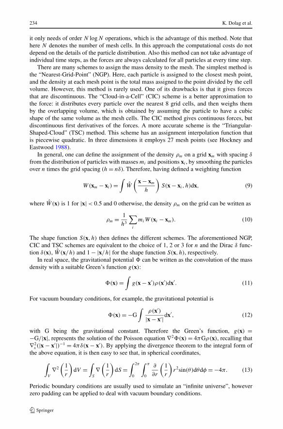
Fig. 6 Mean inner densitycontrast as a function of theenclosed number of particles in4 series of simulations varyingthe number of particles in thehigh-resolution box, from 323

to 2563. Each symbolcorresponds to a fixed fraction ofthe virial radius, as shown by thelabels on the right. The numberof particles needed to obtainrobust results increases withdensity contrast, roughly asprescribed by the requirementthat the collisional relaxationtimescale should remain longerthan the age of the Universe.According to this, robustnumerical estimates of the massprofile of a halo are only possibleto the right of the curve labelledtrelax ∼ 0.6t0. Taken from Poweret al. (2003)

Recently, Power et al. (2003) performed a comprehensive series of convergence tests de-signed to study the effect of numerical parameters on the structure of simulated CDM halos.These tests explore the influence of the gravitational softening, the time stepping algorithm,the starting redshift, the accuracy of force computations, and the number of particles in thespherically-averaged mass profile of a galaxy-sized halo in the CDM cosmogony with anon-null cosmological constant (�CDM). Power et al. (2003), and the references therein,suggest empirical rules that optimise the choice of these parameters. When these choicesare dictated by computational limitations, Power et al. (2003) offer simple prescriptions toassess the effective convergence of the mass profile of a simulated halo. One of their mainresults is summarised in Fig. 6, which shows the convergence of a series of simulations withdifferent mass resolution on different parts of the density profile of a collapsed object. Thisfigure clearly demonstrates that the number of particles within a certain radius needed toobtain converging results depends on the enclosed density.

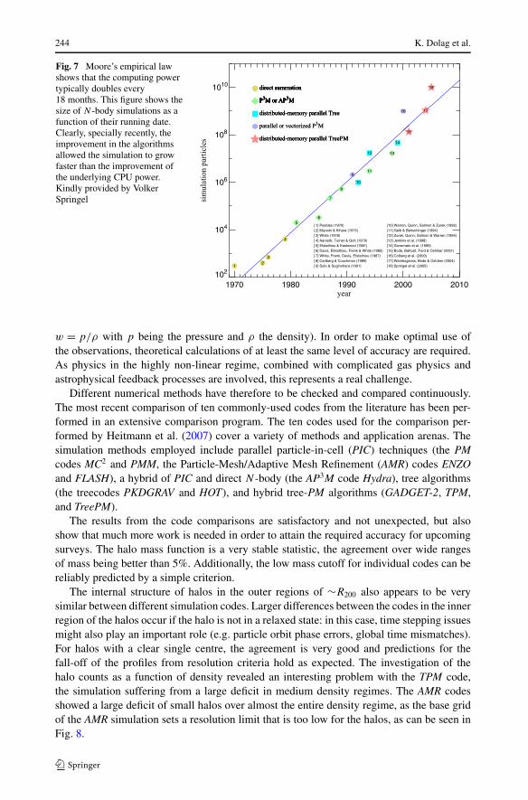
In general, both the size and the dynamical range or resolution of the simulations havebeen increasing very rapidly over the last decades. Figure 7 shows a historical compilationof large N -body simulations: their size growth, thanks to improvements in the algorithms,is faster than the underlying growth of the available CPU power.

2.8 Code Comparison for Pure Gravity

In the last thirty years cosmology has turned from a science of order-of-magnitude estimatesto a science with accuracies of 10% or less in its measurements and theoretical predictions.Crucial observations along the way were the measurement of the cosmic microwave back-ground radiation, and large galaxy surveys. In the future such observations will yield evenhigher accuracy (1%) over a much wider dynamical range. Such measurements will provideinsight into several topics, e.g. the nature of dark energy (expressed by the equation of state

244 K. Dolag et al.

Fig. 7 Moore’s empirical lawshows that the computing powertypically doubles every18 months. This figure shows thesize of N -body simulations as afunction of their running date.Clearly, specially recently, theimprovement in the algorithmsallowed the simulation to growfaster than the improvement ofthe underlying CPU power.Kindly provided by VolkerSpringel

w = p/ρ with p being the pressure and ρ the density). In order to make optimal use ofthe observations, theoretical calculations of at least the same level of accuracy are required.As physics in the highly non-linear regime, combined with complicated gas physics andastrophysical feedback processes are involved, this represents a real challenge.

Different numerical methods have therefore to be checked and compared continuously.The most recent comparison of ten commonly-used codes from the literature has been per-formed in an extensive comparison program. The ten codes used for the comparison per-formed by Heitmann et al. (2007) cover a variety of methods and application arenas. Thesimulation methods employed include parallel particle-in-cell (PIC) techniques (the PMcodes MC2 and PMM, the Particle-Mesh/Adaptive Mesh Refinement (AMR) codes ENZOand FLASH), a hybrid of PIC and direct N -body (the AP3M code Hydra), tree algorithms(the treecodes PKDGRAV and HOT), and hybrid tree-PM algorithms (GADGET-2, TPM,and TreePM).

The results from the code comparisons are satisfactory and not unexpected, but alsoshow that much more work is needed in order to attain the required accuracy for upcomingsurveys. The halo mass function is a very stable statistic, the agreement over wide rangesof mass being better than 5%. Additionally, the low mass cutoff for individual codes can bereliably predicted by a simple criterion.

The internal structure of halos in the outer regions of ∼R200 also appears to be verysimilar between different simulation codes. Larger differences between the codes in the innerregion of the halos occur if the halo is not in a relaxed state: in this case, time stepping issuesmight also play an important role (e.g. particle orbit phase errors, global time mismatches).For halos with a clear single centre, the agreement is very good and predictions for thefall-off of the profiles from resolution criteria hold as expected. The investigation of thehalo counts as a function of density revealed an interesting problem with the TPM code,the simulation suffering from a large deficit in medium density regimes. The AMR codesshowed a large deficit of small halos over almost the entire density regime, as the base gridof the AMR simulation sets a resolution limit that is too low for the halos, as can be seen inFig. 8.


Fig. 8 A recent comparison of the predicted number of halos as a function of density for ten differentcosmological codes. Left panel: halos with 10–40 particles, right panel: halos with 41–2500 particles. Thelower panels show the residuals with respect to GADGET-2. Both panels show the deficit of small halos inENZO and FLASH over most of the density region—only at very high densities do the results catch up. Thebehaviour of the TPM simulation is interesting: not only does this simulation have a deficit of small halosbut the deficit is very significant in medium density regions, in fact falling below the two Adaptive MeshRefinement codes. The slight excess of small halos shown in the TreePM run vanishes completely if the halocut is raised to 20 particles per halo and the TreePM results are in that case in excellent agreement withGADGET-2. Adapted from Heitmann et al. (2007)

The power spectrum measurements revealed definitively more scatter among the differentcodes than expected. The agreement in the nonlinear regime is at the 5–10% level, evenon moderate spatial scales around k = 10h Mpc−1. This disagreement on small scales isconnected to differences of the codes in the inner regions of the halos. For more detaileddiscussion see Heitmann et al. (2007) and references therein.

In a detailed comparison of ENZO and GADGET, O’Shea et al. (2005) already pointedout that to reach reasonable good agreement, relatively conservative criteria for the adaptivegrid refinement are needed. Furthermore, choosing a grid resolution twice as high as themean inter-particle distance of the dark matter particles is recommended, to improve thesmall scale accuracy of the calculation of the gravitational forces.

3 Hydro Methods

The baryonic content of the Universe can typically be described as an ideal fluid. There-fore, to follow the evolution of the fluid, one usually has to solve the set of hydrodynamicequations

dvdt

= −∇P

ρ− ∇�, (47)

246 K. Dolag et al.

dρ

dt+ ρ∇v = 0 (48)

and

du

dt= −P

ρ∇ · v − �(u,ρ)

ρ, (49)

which are the Euler equation, continuity equation and the first law of thermodynamics, re-spectively. They are closed by an equation of state, relating the pressure P to the internalenergy (per unit mass) u. Assuming an ideal, monatomic gas, this will be

P = (γ − 1)ρu (50)

with γ = 5/3. In the next sections, we will discuss how to solve this set of equations, ne-glecting radiative losses described by the cooling function �(u,ρ); in Sect. 4.1 we will giveexamples of how radiative losses or additional sources of heat are included in cosmologicalcodes. We can also assume that the ∇� term will be solved using the methods described inthe previous section.

As a result of the high nonlinearity of gravitational clustering in the Universe, thereare two significant features emerging in cosmological hydrodynamic flows; these featurespose more challenges than the typical hydrodynamic simulation without self-gravity. Onesignificant feature is the extremely supersonic motion around the density peaks developed bygravitational instability, which leads to strong shock discontinuities within complex smoothstructures. Another feature is the appearance of an enormous dynamic range in space andtime, as well as in the related gas quantities. For instance, the hierarchical structures in thegalaxy distribution span a wide range of length scales, from the few kiloparsecs resolved inan individual galaxy to the several tens of megaparsecs characterising the largest coherentscale in the Universe.

A variety of numerical schemes for solving the coupled system of collisional baryonicmatter and collisionless dark matter have been developed in the past decades. They fall intotwo categories: particle methods, which discretise mass, and grid-based methods, whichdiscretise space. We will briefly describe both methods in the next two sections.

3.1 Eulerian (Grid)

The set of hydrodynamical equations for an expanding Universe reads

∂v∂t

+ 1

a(v · ∇)v + a

av = − 1

aρ∇P − 1

a∇�, (51)

∂ρ

∂t+ 3a

aρ + 1

a∇ · (ρv) = 0 (52)

and

∂

∂t(ρu) + 1

av · ∇(ρu) = −(ρu + P )

(1

a∇ · v + 3

a

a

)(53)

respectively, where the right term in the last equation reflects the expansion in addition tothe usual P dV work.

The grid-based methods solve these equations based on structured or unstructured grids,representing the fluid. One distinguishes primitive variables, which determine the thermody-namic properties, (e.g. ρ, v or P ) and conservative variables which define the conservation


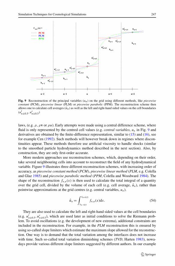
Fig. 9 Reconstruction of the principal variables (un) on the grid using different methods, like piecewiseconstant (PCM), piecewise linear (PLM) or piecewise parabolic (PPM). The reconstruction scheme thenallows one to calculate cell averages (un) as well as the left and right-hand sided values on the cell boundaries(ul

n±0.5, urn±0.5)

laws, (e.g. ρ, ρv or ρu). Early attempts were made using a central difference scheme, wherefluid is only represented by the centred cell values (e.g. central variables, un in Fig. 9 andderivatives are obtained by the finite-difference representation, similar to (15) and (16), seefor example Cen (1992). Such methods will however break down in regimes where discon-tinuities appear. These methods therefore use artificial viscosity to handle shocks (similarto the smoothed particle hydrodynamics method described in the next section). Also, byconstruction, they are only first-order accurate.

More modern approaches use reconstruction schemes, which, depending on their order,take several neighbouring cells into account to reconstruct the field of any hydrodynamicalvariable. Figure 9 illustrates three different reconstruction schemes, with increasing order ofaccuracy, as piecewise constant method (PCM), piecewise linear method (PLM, e.g. Colellaand Glaz 1985) and piecewise parabolic method (PPM, Colella and Woodward 1984). Theshape of the reconstruction fn,u(x) is then used to calculate the total integral of a quantityover the grid cell, divided by the volume of each cell (e.g. cell average, un), rather thanpointwise approximations at the grid centres (e.g. central variables, un).

un =∫ xn+0.5

xn−0.5

fn,u(x)dx. (54)

They are also used to calculate the left and right-hand sided values at the cell boundaries(e.g. ul

n±0.5, urn±0.5), which are used later as initial conditions to solve the Riemann prob-

lem. To avoid oscillations (e.g. the development of new extrema), additional constraints areincluded in the reconstruction. For example, in the PLM reconstruction this is ensured byusing so-called slope limiters which estimate the maximum slope allowed for the reconstruc-tion. One way is to demand that the total variation among the interfaces does not increasewith time. Such so-called total variation diminishing schemes (TVD, Harten 1983), nowa-days provide various different slope limiters suggested by different authors. In our example

248 K. Dolag et al.

illustrated by Fig. 9, the so called minmod slope limiter

ui = minmod (�(ui+1 − ui), (ui+1 − ui−1)/2, θ(ui − ui−1)) , (55)

where ui is the limiter slope within the cell i and θ = [1,2], would try to fix the slopef ′

n−1,u(xn−1) and f ′n,u(xn), such as to avoid that ul

n−0.5 becomes larger than urn−0.5. The so

called Aldaba-type limiter

ui = 2(ui+1 − ui)(ui − ui−1) + ε

(ui+1 − ui)2 + (ui − ui−1)2 + ε2

1

2(ui+1 − ui−1), (56)

where ε is a small positive number to avoid problems in homogeneous regions, would tryto avoid that ul

n−0.5 is getting larger than un and that urn−0.5 is getting smaller than un−1, e.g.

that a monotonic profile in ui is preserved.In the PPM (or even higher order) reconstruction this enters as an additional condition

when finding the best-fitting polynomial function. The additional cells which are involvedin the reconstruction are often called the stencil. Modern, high order schemes usually havestencils based on at least 5 grid points and implement essentially non-oscillatory (ENO;Harten et al. 1987) or monoticity preserving (MP) methods for reconstruction, which main-tain high-order accuracy. For every reconstruction, a smoothness indicator Sm

n can be con-structed, which is defined as the integral over the sum of the squared derivatives of thereconstruction over the stencil chosen, e.g.

Smn =

2∑l=1

∫ xn+m

xn−m

( x)2l−1(∂l

xfmn,u(x)

)2dV. (57)

In the ENO schemes, a set of candidate polynomials pmn with order 2m + 1 for a set of sten-

cils based on different numbers of grid cells m are used to define several different recon-struction functions f m

n,u. Then, the reconstruction with the lowest smoothness indicator Smn

is chosen. In this way the order of reconstruction will be reduced around discontinuities, andoscillating behaviour will be suppressed.

To improve on the ENO schemes in robustness and accuracy one can, instead of selectingthe reconstruction with the best smoothness indicator Sm

n , construct the final reconstructionby building the weighted reconstruction

fu(x) =∑m

wmf mn,u(x), (58)

where the weights wm are a proper function of the smoothness indicators Smn . This procedure

is not unique. Jiang and Shu (1996) proposed defining

wm = αm∑l αl

(59)

with

αl = Cl

(ε + Sln)

β, (60)

where Cl , ε and β are free parameters, which for example can be taken from Levy et al.(1999). This are the so-called weighted essentially non-oscillatory (WENO) schemes. These


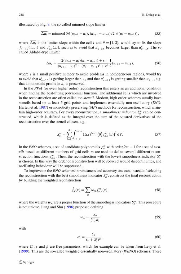
Fig. 10 The Riemann problem:The upper panel shows the initialstate, the lower panel shows theevolved problem for the case ofno relative motion between thetwo sides (u1 = u5 = 0). Thesolid lines mark the pressure P ,the dashed dotted lines thedensity ρ and the dotted line thevelocity v. Kindly provided byEwald Müller

schemes can simultaneously provide a high-order resolution for the smooth part of the solu-tion and a sharp, monotonic shock or contact discontinuity transition. For a review on ENOand WENO schemes, see e.g. Shu (1998).

After the left and right-hand values at the cell boundaries (e.g. interfaces) are recon-structed, the resulting Riemann problem is solved, e.g. the evolution of two constant statesseparated by a discontinuity. This can be done either analytically or approximately, usingleft and right-handed values at the interfaces as a jump condition.

With the solution one obtains, the fluxes across these boundaries for the time step can becalculated and the cell averages un can be updated accordingly. In multiple dimensions, allthese steps are performed for each coordinate direction separately, taking only the interfacevalues along the individual axes into account. There are attempts to extend the reconstruc-tion schemes, to directly reconstruct the principal axis of the Riemann problem in multipledimensions, so that then it has to be solved only once for each cell. However the complexityof reconstructing the surface of shocks in three dimensions has so far seen to be untraceable.

How to solve the general Riemann problem, e.g. the evolution of a discontinuity initiallyseparating two states, can be found in text books (e.g. Courant and Friedrichs 1948). Herewe give only the evolution of a shock tube as an example. This corresponds to a systemwhere both sides are initially at rest. Figure 10 shows the initial and the evolved system. Thelatter can be divided into 5 regions. The values for regions 1 and 5 are identical to the initialconfiguration. Region 2 is a rarefaction wave which is determined by the states in regions 1and 3. Therefore we are left with 6 variables to determine, namely ρ3, P3, v3 and ρ4, P4, v4,where we have already eliminated the internal energy ui in all regions, as it can be calculatedfrom the equation of state. As there is no mass flux through the contact discontinuity, andas the pressure is continuous across the contact discontinuity, we can eliminate two of thesix variables by setting v3 = v4 = vc and P3 = P4 = Pc. The general Rankine-Hugoniotconditions, describing the jump conditions at a discontinuity, read

ρlvl = ρrvr (61)

250 K. Dolag et al.

ρlv2l + Pl = ρrv

2r + Pr (62)

vl

(ρl(v

2l /2 + ul) + Pl

) = vr

(ρr(v

2r /2 + ur) + Pr

), (63)

where we have assumed a coordinate system which moves with the shock velocity vs.Assuming that the system is at rest in the beginning, e.g. v1 = v5 = 0, the first Rankine-Hugoniot condition for the shock between region 4 and 5 moving with a velocity vs (notethe implied change of the coordinate system) is in our case

m = ρ5vs = ρ4(vs − vc) (64)

and therefore the shock velocity becomes

vs = ρ4vc

ρ4 − ρ5. (65)

The second Rankine-Hugoniot condition is

mvc = ρ4(vs − vc)vc = Pc − P5, (66)

which, combined with the first, can be written as

ρ4

(ρ4vc

ρ4 − ρ5− vc

)vc = Pc − P5, (67)

which, slightly simplified, leads to a first condition

(P5 − Pc)

(1

ρ5− 1

ρ4

)= −v2

c . (68)

The third Rankine-Hugoniot condition is

m

(ε4 + v2

c

2− ε5

)= Pcvc, (69)

which, by eliminating m, can be written as

ε4 − ε5 = Pc + P5

Pc − P5

v2c

2. (70)

Using the first condition (68) and assuming an ideal gas for the equation of state, one gets

1

γ − 1

(Pc

ρ4− P5

ρ5

)= Pc + P5

2ρ4ρ5, (71)

which leads to the second condition

Pc − P5

Pc + P5= γ

ρ4 − ρ5

ρ4 + ρ5. (72)

The third condition comes from the fact that the entropy (∝ ln(P/ργ ) stays constant in therarefaction wave, and therefore one can write it as

P1

Pc=

(ρ1

ρ3

)γ

. (73)


The fourth condition comes from the fact that the Riemann Invariant

v +∫

c

ρdρ (74)

is a constant, which means that

vc +∫

c3

ρ3dρ = v1 +

∫c1

ρ1dρ, (75)

where c = √γP/ρ denotes the sound velocity, with which the integral can be written as

∫c

ρdρ = 2

γ − 1

√γP

ρ. (76)

Therefore, the fourth condition can be written as

vc + 2

γ − 1

√γPc

ρ3= 2

γ − 1

√γP1

ρ1. (77)

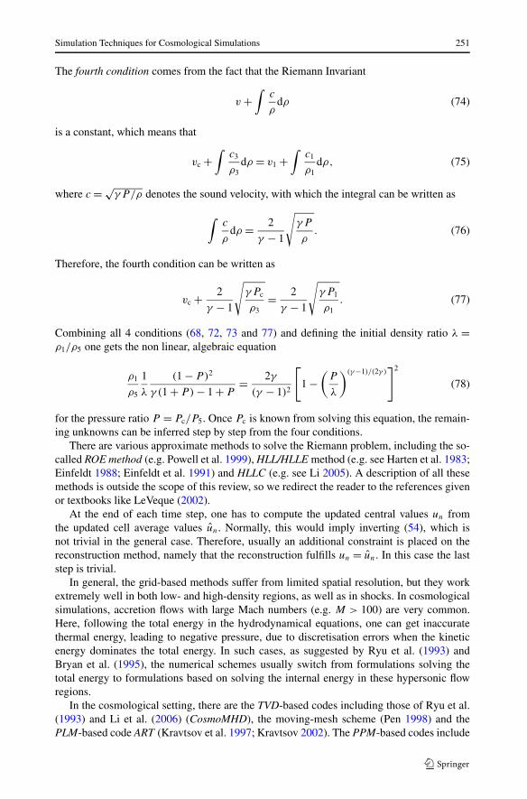
Combining all 4 conditions (68, 72, 73 and 77) and defining the initial density ratio λ =ρ1/ρ5 one gets the non linear, algebraic equation

ρ1

ρ5

1

λ

(1 − P )2

γ (1 + P ) − 1 + P= 2γ

(γ − 1)2

[1 −

(P

λ

)(γ−1)/(2γ )]2

(78)

for the pressure ratio P = Pc/P5. Once Pc is known from solving this equation, the remain-ing unknowns can be inferred step by step from the four conditions.

There are various approximate methods to solve the Riemann problem, including the so-called ROE method (e.g. Powell et al. 1999), HLL/HLLE method (e.g. see Harten et al. 1983;Einfeldt 1988; Einfeldt et al. 1991) and HLLC (e.g. see Li 2005). A description of all thesemethods is outside the scope of this review, so we redirect the reader to the references givenor textbooks like LeVeque (2002).

At the end of each time step, one has to compute the updated central values un fromthe updated cell average values un. Normally, this would imply inverting (54), which isnot trivial in the general case. Therefore, usually an additional constraint is placed on thereconstruction method, namely that the reconstruction fulfills un = un. In this case the laststep is trivial.

In general, the grid-based methods suffer from limited spatial resolution, but they workextremely well in both low- and high-density regions, as well as in shocks. In cosmologicalsimulations, accretion flows with large Mach numbers (e.g. M > 100) are very common.Here, following the total energy in the hydrodynamical equations, one can get inaccuratethermal energy, leading to negative pressure, due to discretisation errors when the kineticenergy dominates the total energy. In such cases, as suggested by Ryu et al. (1993) andBryan et al. (1995), the numerical schemes usually switch from formulations solving thetotal energy to formulations based on solving the internal energy in these hypersonic flowregions.

In the cosmological setting, there are the TVD-based codes including those of Ryu et al.(1993) and Li et al. (2006) (CosmoMHD), the moving-mesh scheme (Pen 1998) and thePLM-based code ART (Kravtsov et al. 1997; Kravtsov 2002). The PPM-based codes include

252 K. Dolag et al.

those of Stone and Norman (1992) (Zeus), Bryan et al. (1995) (ENZO), Ricker et al. (2000)(COSMOS) and Fryxell et al. (2000) (FLASH). There is also the WENO-based code by Fenget al. (2004).

3.2 Lagrangian (SPH)

The particle methods include variants of smoothed particle hydrodynamics (SPH; Gingoldand Monaghan 1977; Lucy 1977) such as those of Evrard (1988), Hernquist and Katz (1989),Navarro and White (1993), Couchman et al. (1995) (Hydra), Steinmetz (1996a) (GRAPE-SPH), Owen et al. (1998), and Springel et al. (2001a), Springel (2005) (GADGET). TheSPH method solves the Lagrangian form of the Euler equations and can achieve good spa-tial resolutions in high-density regions, but it works poorly in low-density regions. It alsosuffers from degraded resolution in shocked regions due to the introduction of a sizable arti-ficial viscosity. Agertz et al. (2007) argued that whilst Eulerian grid-based methods are ableto resolve and treat dynamical instabilities, such as Kelvin-Helmholtz or Rayleigh-Taylor,these processes are poorly resolved by existing SPH techniques. The reason for this is thatSPH, at least in its standard implementation, introduces spurious pressure forces on particlesin regions where there are steep density gradients, in particular near contact discontinuities.This results in a boundary gap of the size of an SPH smoothing kernel radius, over whichinteractions are severely damped. Nevertheless, in the cosmological context, the adaptivenature of the SPH method compensates for such shortcomings, thus making SPH the mostcommonly used method in numerical hydrodynamical cosmology.

3.2.1 Basics of SPH

The basic idea of SPH is to discretise the fluid by mass elements (e.g. particles), rather thanby volume elements as in the Eulerian methods. Therefore it is immediately clear that themean inter-particle distance in collapsed objects will be smaller than in underdense regions;the scheme will thus be adaptive in spatial resolution by keeping the mass resolution fixed.For a comprehensive review see Monaghan (1992). To build continuous fluid quantities, onestarts with a general definition of a kernel smoothing method

〈A(x)〉 =∫

W(x − x′, h)A(x′)dx′, (79)

which requires that the kernel is normalised (i.e.∫

W(x, h)dx = 1) and collapses to a deltafunction if the smoothing length h approaches zero, namely W(x, h) → δ(x) for h → 0.

One can write down the continuous fluid quantities (e.g. 〈A(x)〉) based on the discretisedvalues Aj represented by the set of the individual particles mj at the position xj as

〈Ai〉 = 〈A(xi )〉 =∑

j

mj

ρj

AjW(xi − xj , h) , (80)

where we assume that the kernel depends only on the distance modulus (i.e. W(|x − x′|, h))and we replace the volume element of the integration, dx = d3x, with the ratio of the massand density mj/ρj of the particles. Although this equation holds for any position x in space,here we are only interested in the fluid representation at the original particle positions xi ,which are the only locations where we will need the fluid representation later on. It is im-portant to note that for kernels with compact support (i.e. W(x, h) = 0 for |x| > h) thesummation does not have to be done over all the particles, but only over the particles within


the sphere of radius h, namely the neighbours around the particle i under consideration.Traditionally, the most frequently used kernel is the B2-spline, which can be written as

W(x,h) = σ

hν

⎧⎪⎪⎪⎪⎪⎨⎪⎪⎪⎪⎪⎩

1 − 6(x

h

)2 + 6(x

h

)3, 0 ≤ x

h< 0.5,

2(

1 − x

h

)3, 0.5 ≤ x

h< 1,

0, 1 ≤ x

h,

(81)

where ν is the dimensionality (e.g. 1, 2 or 3) and σ is the normalisation

σ =

⎧⎪⎪⎪⎪⎪⎨⎪⎪⎪⎪⎪⎩

16

3, ν = 1,

80

7π, ν = 2,

8

π, ν = 3.

(82)

Sometimes, spline kernels of higher order are used for very special applications; howeverthe B2 spline kernel turns out to be the optimal choice in most cases.

When one identifies Ai with the density ρi , ρi cancels out on the right hand side of (80),and we are left with the density estimate

〈ρi〉 =∑

j

mjW(xi − xj , h), (83)

which we can interpret as the density of the fluid element represented by the particle i.Now even derivatives can be calculated as

∇ 〈Ai〉 =∑

j

mj

ρj

Aj∇iW(xi − xj , h), (84)

where ∇i denotes the derivative with respect to xi . A pairwise symmetric formulation ofderivatives in SPH can be obtained by making use of the identity

(ρ∇) · A = ∇(ρ · A) − ρ · (∇A), (85)

which allows one to re-write a derivative as

∇ 〈Ai〉 = 1

ρi

∑j

mj (Aj − Ai)∇iW(xi − xj , h). (86)

Another way of symmetrising the derivative is to use the identity

∇A

ρ= ∇

(A

ρ

)+ A

ρ2∇ρ, (87)

which then leads to the following form of the derivative:

∇ 〈Ai〉 = ρi

∑j

mj

(Aj

ρ2j

+ Ai

ρ2i

)∇iW(xi − xj , h). (88)

254 K. Dolag et al.

3.2.2 The Fluid Equations

By making use of these identities, the Euler equation can be written as

dvi

dt= −

∑j

mj

(Pj

ρ2j

+ Pi

ρ2i

+ �ij

)∇iW(xi − xj , h). (89)

By combining the above identities and averaging the result, the term −(P/ρ)∇ · v from thefirst law of thermodynamics can similarly be written as

dui

dt= 1

2

∑j

mj

(Pj

ρ2j

+ Pi

ρ2i

+ �ij

)(vj − vi

)∇iW(xi − xj , h). (90)

Here we have added a term �ij which is the so-called artificial viscosity. This term isusually needed to capture shocks and its construction is similar to other hydro-dynamicalschemes. Usually, one adopts the form proposed by Monaghan and Gingold (1983) and Bal-sara (1995), which includes a bulk viscosity and a von Neumann-Richtmeyer viscosity term,supplemented by a term controlling angular momentum transport in the presence of shearflows at low particle numbers (Steinmetz 1996b). Modern schemes implement a form ofthe artificial viscosity as proposed by Monaghan (1997) based on an analogy with Riemannsolutions of compressible gas dynamics. To reduce this artificial viscosity, at least in thoseparts of the flows where there are no shocks, one can follow the idea proposed by Morrisand Monaghan (1997): every particle carries its own artificial viscosity, which eventuallydecays outside the regions which undergo shocks. A detailed study of the implications onthe ICM of such an implementation can be found in Dolag et al. (2005).

The continuity equation does not have to be evolved explicitly, as it is automaticallyfulfilled in Lagrangian methods. As shown earlier, density is no longer a variable but canbe, at any point, calculated from the particle positions. Obviously, mass conservation isguaranteed, unlike volume conservation: in other words, the sum of the volume elementsassociated with all of the particles might vary with time, especially when strong densitygradients are present.

3.2.3 Variable Smoothing Length

Usually, the smoothing length h will be allowed to vary for each individual particle i andis determined by finding the radius hi of a sphere which contains n neighbours. Typically,different numbers n of neighbours are chosen by different authors, ranging from 32 to 80.In principle, depending on the kernel, there is an optimal choice of neighbours (e.g. seeSilverman 1986 or similar books). However, one has to find a compromise between a largenumber of neighbours, leading to larger systematics but lower noise in the density esti-mates (especially in regions with large density gradients) and a small number of neigh-bours, leading to larger sample variances for the density estimation. In general, once everyparticle has its own smoothing length, a symmetric kernel W(xi − xj , hi, hj ) = Wij hasto be constructed to keep the conservative form of the formulations of the hydrodynami-cal equations. There are two main variants used in the literature: one is the kernel averageWij = (W(xi − xj , hi)+W(xi − xj , hj ))/2, the other is an average of the smoothing lengthWij = W(xi − xj , (hi + hj )/2). The former is the most commonly used approach.

Note that in all of the derivatives discussed above, it is assumed that h does not de-pend on the position xj . Thus, by allowing the smoothing length hi to be variable for each


particle, one formally neglects the correction term ∂W/∂h, which would appear in all thederivatives. In general, this correction term cannot be computed trivially and therefore manyimplementations do not take it into account. It is well known that such formulations are poorat conserving numerically both internal energy and entropy at the same time, independentlyof the use of internal energy or entropy in the formulation of the first law of thermodynam-ics, see Hernquist (1993). In the next subsection, we present a way of deriving the equationswhich include these correction terms ∂W/∂h; this equation set represents a formulationwhich conserves numerically both entropy and internal energy.

3.2.4 The Entropy Conservation Formalism

To derive a better formulation of the SPH method, Springel and Hernquist (2002) startedfrom the entropic function A = P/ργ , which will be conserved in adiabatic flows. Theinternal energy per unit mass can be inferred from this entropic function as

ui = Ai

γ − 1ρ

γ−1i (91)

at any time, if needed. Entropy will be generated by shocks, which are captured by theartificial viscosity �ij and therefore the entropic function will evolve as

dAi

dt= 1

2

γ − 1

ργ−1i

∑j

mj�ij

(vj − vi

)∇iWij . (92)

The Euler equation can be derived starting by defining the Lagrangian of the fluid as

L(q, q) = 1

2

∑i

mi x2i − 1

γ − 1

∑i

miAiργ−1i (93)

which represents the entire fluid and has the coordinates q = (x1, . . . ,xN,h1, . . . , hN). Thenext important step is to define constraints, which allow an unambiguous association of hi

for a chosen number of neighbours n. This can be done by requiring that the kernel volumecontains a constant mass for the estimated density,

φi(q) = 4π

3h3

i ρi − nmi = 0. (94)

The equation of motion can be obtained as the solution of

d

dt

∂L

∂qi

− ∂L

∂qi

=∑

j

λj

∂φj

∂qi

, (95)

which—as demonstrated by Springel and Hernquist (2002)—can be written as

dvi

dt= −

∑j

mj

(fj

Pj

ρ2j

∇iW(xi − xj , hj ) + fi

Pi

ρ2i

∇iW(xi − xj , hi) + �ij∇iWij

), (96)

where we already have included the additional term due to the artificial viscosity �ij , whichis needed to capture shocks. The coefficients fi incorporate fully the variable smoothing

256 K. Dolag et al.

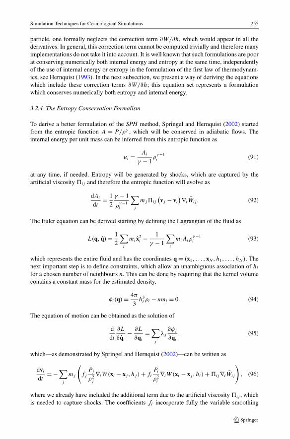
Fig. 11 One-dimensional velocity dispersion profile (left panel) and gas temperature profile (right panel) ofthe cluster at z = 0 of the Santa Barbara Comparison Project (Frenk et al. 1999). The solid line is the profileaveraged over the 12 simulations. The symbols correspond to individual simulations. The crosses in the leftpanel correspond to a dark-matter only simulation. The top panels show the residual from the mean profile.Taken from Frenk et al. (1999)

length correction term and are defined as

fi =(

1 + hi

3ρi

∂ρi

∂hi

)−1

. (97)

Note that in addition to the correction terms, which can be easily calculated together withthe density estimation, this formalism also avoids all the ambiguities we saw in the deriva-tions of the equations in the previous section. This formalism defines how the kernel av-erages (symmetrisation) have to be taken, and also fixes hi to unambiguous values. For adetailed derivation of this formalism and its conserving capabilities see Springel and Hern-quist (2002).

3.3 Code Comparison

The Eulerian and Lagrangian approaches described in the previous sections should providethe same results when applied to the same problem, like the interaction of multi-phase fluids(Agertz et al. 2007). To verify that the code correctly solves the hydrodynamical set ofequations, each code is usually tested against problems whose solution is known analytically.In practise, these are shock tubes or spherical collapse problems. In cosmology, a relevanttest is to compare the results provided by the codes when they simulate the formation ofcosmic structure, when finding an analytic solution is impractical; for example O’Shea et al.(2005) compare the thermodynamical properties of the intergalactic medium predicted bythe GADGET (SPH-based) and ENZO (grid-based) codes. Another example of a comparisonbetween grid-based and SPH-based codes can be found in Kang et al. (1994).

A detailed comparison of hydrodynamical codes which simulate the formation and evo-lution of a cluster was provided by the Santa Barbara Cluster Comparison Project (Frenk


et al. 1999). Frenk et al. (1999) comprised 12 different groups, each using a code eitherbased on the SPH technique (7 groups) or on the grid technique (5 groups). Each simulationstarted with identical initial conditions of an individual massive cluster in a flat CDM modelwith zero cosmological constant. Each group was free to decide resolution, boundary condi-tions and the other free parameters of their code. The simulations were performed ignoringradiative losses and the simulated clusters were compared at z = 0.5 and z = 0.

The resulting dark matter properties were similar: it was found a 20% scatter around themean density and velocity dispersion profiles (left panel of Fig. 11). A similar agreementwas also obtained for many of the gas properties, like the temperature profile (right panel ofFig. 11) or the ratio of the specific dark matter kinetic energy and the gas thermal energy.

Somewhat larger differences are present for the inner part of the temperature or entropyprofiles and more recent implementations have not yet cured this problem. The largest dis-crepancy was in the total X-ray luminosity. This quantity is proportional to the square ofthe gas density, and resolving the cluster central region within the core radius is crucial:the simulations resolving this region had a spread of 2.6 in the total X-ray luminosity,compared to a spread of 10 when all the simulations were included. Frenk et al. (1999)also concluded that a large fraction of the discrepancy, when excluding the X-ray lumi-nosity result, was due to differences in the internal timing of the simulations: these dif-ferences produce artificial time shifts between the outputs of the various simulations evenif the outputs are formally at the same cosmic time. This reflects mainly the underly-ing dark matter treatment, including chosen force accuracy, different integration schemesand choice of time steps used, as described in the previous sections. A more worrisomedifference between the different codes is the predicted baryon fraction and its profilewithin the cluster. Here modern schemes still show differences (e.g. see Ettori et al. 2006;Kravtsov et al. 2005), which makes it difficult to use simulations to calibrate the systematicsin the cosmological test based on the cluster baryon fraction.

To date, the comparisons described in the literature show a satisfactory agreement be-tween the two approaches, with residual discrepancies originating from the known weak-nesses which are specific to each scheme. A further limitation of these comparisons is that,in most cases, the simulations are non-radiative. However, at the current state of the art, per-forming comparisons of simulations including radiative losses is not expected to provide ro-bust results. As described in the next section, the first relevant process that needs to be addedis radiative cooling: however, depending on the square of the gas density, cooling increaseswith resolution without any indication of convergence, see for example Fig. 13, taken fromBorgani et al. (2006). At the next level of complexity, star formation and supernova feed-back occur in regions which have a size many orders of magnitude smaller than the spatialresolution of the cosmological simulations. Thus, simulations use phenomenological recipesto describe these processes, and any comparison would largely test the agreement betweenthese recipes rather than identify the inadequacy of the numerical integration schemes.

4 Adding Complexity

In this section, we will give a brief overview of how astrophysical processes, that go beyondthe description of the gravitational instability and of the hydrodynamical flows are usuallyincluded in simulation codes.

4.1 Cooling

We discuss here how the �(u,ρ) term is usually added in the first law of thermodynamics,described by (49), and its consequences.

258 K. Dolag et al.

Fig. 12 The top panel shows thetotal cooling curve (solid line)and its composition fromdifferent processes for aprimordial mixture of H and He.The bottom panel shows how thetotal cooling curve will change asa function of different metallicity,as indicated in the plot(in absolute values). The partbelow 104 K also takes intoaccount cooling by molecules(e.g. HD and H2) and metal lines.Taken from Maio et al. (2007)

In cosmological applications, one is usually interested in structures with virial tempera-tures larger than 104 K. In standard implementations of the cooling function �(u,ρ), oneassumes that the gas is optically thin and in ionisation equilibrium. It is also usually as-sumed that three-body cooling processes are unimportant, so as to restrict the treatment totwo-body processes. For a plasma with primordial composition of H and He, these processesare collisional excitation of H I and He II, collisional ionisation of H I, He I and He II, stan-dard recombination of H II, He II and He III, dielectric recombination of He II, and free-freeemission (Bremsstrahlung). The collisional ionisation and recombination rates depend only


Fig. 13 The fraction of cooledbaryons fc as a function of themass of the gas particle, for4 different clusters at differentresolutions is shown. Filledsymbols are for the runs includingkinetic feedback (e.g. winds), theopen circles are re-simulations ofone of the clusters with windfeedback turned off. The asteriskis for one of the clusters run atvery high resolution using fewer,but 8 times heavier, gas particlesthan normal, so that the gasparticle mass is similar to that ofthe DM particles in thehigh-resolution region. Takenfrom Borgani et al. (2006)

on temperature. Therefore, in the absence of ionising background radiation one can solvethe resulting rate equation analytically. This leads to a cooling function �(u)/ρ2 as illus-trated in the top panel of Fig. 12. In the presence of ionising background radiation, therate equations can be solved iteratively. Note that for a typical cosmological radiation back-ground (e.g. UV background from quasars, see Haardt and Madau 1996), the shape of thecooling function can be significantly altered, especially at low densities. For a more de-tailed discussion see for example Katz et al. (1996). Additionally, the presence of metalswill drastically increase the possible processes by which the gas can cool. As it becomescomputationally very demanding to calculate the cooling function in this case, one usuallyresorts to a pre-computed, tabulated cooling function. As an example, the bottom panel ofFig. 12, at temperatures above 105 K, shows the tabulated cooling function by Sutherlandand Dopita (1993) for different metallicities of the gas, keeping the ratios of the differentmetal species fixed to solar values. Note that almost all implementations solve the aboverate equations (and therefore the cooling of the gas) as a “sub time step” problem, decou-pled from the hydrodynamical treatment. In practise this means that one assumes that thedensity is fixed across the time step. Furthermore, the time step of the underlying hydrody-namical simulation are in general, for practical reasons, not controlled by or related to thecooling time-scale. The resulting uncertainties introduced by these approximations have notyet been deeply explored and clearly leave room for future investigations.

For the formation of the first objects in halos with virial temperatures below 104 K, theassumption of ionisation equilibrium no longer holds. In this case, one has to follow the non-equilibrium reactions, solving the balance equations for the individual levels of each speciesduring the cosmological evolution. In the absence of metals, the main coolants are H2 andH+

2 molecules (see Abel et al. 1997). HD molecules can also play a significant role. Whenmetals are present, many more reactions are available and some of these can contributesignificantly to the cooling function below 104 K. This effect is clearly visible in the bottompanel of Fig. 12, for T < 104 K. For more details see Galli and Palla (1998) or Maio et al.(2007) and references therein.

260 K. Dolag et al.

4.2 Star Formation and Feedback

Including radiative losses in simulations causes two numerical problems. Firstly, coolingis a runaway process and, at the typical densities reached at the centres of galaxy clusters,the cooling time becomes significantly shorter than the Hubble time. As a consequence, alarge fraction of the baryonic component can cool down and condense out of the hot phase.Secondly, since cooling is proportional to the square of the gas density, its efficiency is quitesensitive to the presence of the first collapsing small halos, where cooling takes place, andtherefore on numerical resolution.

To deal with these issues, one has to include in the code a suitable recipe to convert thereservoir of cold and dense gas into collisionless stars. Furthermore, this stellar componentshould represent the energy feedback from supernova explosions, which ideally would heatthe cold gas, so as to counteract the cooling catastrophe.

As for star formation, a relatively simple recipe is that originally introduced by (Katzet al. 1996), which is often used in cosmological simulations. According to this prescription,for a gas particle to be eligible to form stars, it must have a convergent flow,

∇vi < 0 , (98)

and have density in excess of some threshold value, e.g.

ρi > 0.1 atoms cm−3. (99)

These criteria are complemented by requiring the gas to be Jeans unstable, that is

hi

ci

>1√

4πGρi

, (100)

where hi is either the SPH smoothing length or the mesh size for Eulerian codes and ci is thelocal sound speed. This indicates that the individual resolution element gets gravitationallyunstable. At high redshift, the physical density can easily exceed the threshold given in (99),even for particles not belonging to virialised halos. Therefore one usually applies a furthercondition on the gas overdensity,

ρi

ρmean> 55.7, (101)

which restricts star formation to collapsed, virialised regions. Note that the density criterionis the most important one. Particles fulfilling it in almost all cases also fulfill the other twocriteria.

Once a gas particle is eligible to form stars, its star formation rate can be written as

dρ∗dt

= −dρi

dt= c∗ρi

t∗, (102)

where c∗ is a dimensionless star formation rate parameter and t∗ the characteristic timescalefor star formation. The value of this timescale is usually taken to be the maximum of thedynamical time tdyn = (4πGρi)

−0.5 and the cooling time tcool = ui/(dui/dt). In principle,to follow star formation, one would like to produce continuously collisionless star parti-cles. However, for computational and numerical reasons, one approximates this process bywaiting for a significant fraction of the gas particle mass to have formed stars accordingto the above rate; when this is accomplished, a new, collisionless “star” particle is created


from the parent star-forming gas particle, whose mass is reduced accordingly. This processtakes place until the gas particle is entirely transformed into stars. In order to avoid spuri-ous numerical effects, which arise from the gravitational interaction of particles with widelydiffering masses, one usually restricts the number of star particles (so called generations)spawned by a gas particle to be relatively small, typically 2–3. Note that it is also commonto restrict the described star-formation algorithm to only convert a gas particle into a starparticle, which correspond to the choice of only one generation. In this case star and gasparticles have always the same mass.

To get a more continuous distribution of star particle masses, the probability of forminga star can be written as

p = 1 − exp

(−c∗

t

tg

)(103)

and a random number is used to decide when to form a star particle.According to this scheme of star formation, each star particle can be identified with a

Simple Stellar Population (SSP), i.e. a coeval population of stars characterised by a givenassumed initial mass function (IMF). Further, assuming that all stars with masses larger than8 M� will end as type-II supernovae (SN II), one can calculate the total amount of energy(typically 1051 erg per supernova) that each star particle can release to the surrounding gas.Under the approximation that the typical lifetime of massive stars which explode as SN IIdoes not exceed the typical time step of the simulation, this is done in the so-called “instan-taneous recycling approximation”, with the feedback energy deposited in the surroundinggas in the same step.

Improvements with respect to this model include an explicit sub-resolution descriptionof the multi-phase nature of the interstellar medium, which provides the reservoir of starformation. Such a sub grid model tries to model the global dynamical behaviour of theinterstellar medium in which cold, star-forming clouds are embedded in a hot medium.

One example is the multi-phase sub-grid model suggested by Springel and Hernquist(2003), in which a star-forming gas particle has a multi-phase nature, with a cold phasedescribing cold clouds embedded in pressure equilibrium within a hot medium. Accordingto this model, star formation takes place in a self-regulated way. Within this model (as withinother models), part of the feedback energy is channelled back into kinetic energy, effectivelyleading to a quasi self-consistent modelling of galactic outflows, driven by the star-formingregions. Once an efficient form of kinetic feedback is included, the amount of stars formedin simulations turns out to converge when resolution is varied. An example of the predictedstellar component in different galaxy clusters for varying spatial resolutions, taken fromBorgani et al. (2006) is shown in Fig. 13.

A further direction for improvement is provided by a more accurate description of stel-lar evolution, and of the chemical enrichment associated with star forming particles. Moreaccurate models require that energy feedback and metals are released not just by SN II, butalso by SN Ia and low and intermediate mass stars, thereby avoiding the instantaneous recy-cling approximation (e.g., see Borgani et al. 2008—Chap. 18, this issue, for a more detaileddiscussion of this point).

4.3 Additional Physics

A number of other physical processes, besides those related to star formation and SN feed-back, are in general expected to play a role in the evolution of the cosmic baryons and, assuch, should be added into the treatment of the hydrodynamical equations. For instance,

262 K. Dolag et al.

Fig. 14 Maps for the SZ decrement for a simulated galaxy cluster. The original map extracted from thehydrodynamic simulation, and the same map in the simulated observation (t = 34 h) which assumes the AMIinterferometric response, are shown in the left and right panel, respectively. The side of each map correspondsto 16 arcmin. The colour scale is shown at the bottom of each panel. Taken from Bonaldi et al. (2007)

magnetic fields or the effect of a population of relativistic particles as described in detailin the review by Dolag et al. (2008)—Chap. 12, this issue. Other processes, whose effecthas been studied in cosmological simulations of galaxy clusters include thermal conduction(Jubelgas et al. 2004; Dolag et al. 2004), radiative transfer to describe the propagation ofphotons in a medium (e.g. Iliev et al. 2006 and references therein), growth of black holesand the resulting feedback associated with the extracted energy (e.g. Sijacki et al. 2007 andreferences therein). A description of these processes is far outside the scope of this reviewand we point the interested reader to the original papers cited above.

5 Connecting Simulations to Observations

Both the recent generation of instruments and an even more sophisticated next generationof instruments (at various wavelengths) will allow us to study galaxy clusters in rich detail.Therefore, when comparing observations with simulations, instrumental effects like resolu-tion and noise, as well as more subtle effects within the observational processes, have to betaken into account to separate true features from instrumental effects and biases. Therefore,the building up of synthetic instruments to “observe” simulations becomes more and moreimportant.

As an example, Fig. 14 shows the difference between a Sunyaev-Zel’dovich map ob-tained from a simulated galaxy cluster, and how it would be observed with the AMI1 in-strument, assuming the response according to the array configuration of the radio dishesand adding the appropriate noise. Here a 34 hours observation has been assumed, and theCLEAN deconvolution algorithm applied. For details see Bonaldi et al. (2007).

1http://www.mrao.cam.ac.uk/telescope/ami


Fig. 15 Compositeugr + riz + izy image of asimulated galaxy clusterincluding its simulated lensingsignal, having its imprint inseveral strong lensing features.To construct the surfacebrightness distributions of boththe cluster members and of thebackground galaxies, shapeletdecompositions were used. Foreach cluster galaxy themorphological classifications andspectral energy distributioninferred from the semi-analyticmodelling based on the mergertrees from the underlying clustersimulation were used torealistically model the opticalappearance of the cluster. Thefield of view is 100′′ × 100′′ andan exposure of 1000 s for eachband was assumed. Taken fromMeneghetti et al. (2007)

Another example of a synthetic observation by a virtual telescope is shown in Fig. 15,which shows an optical image of a simulated galaxy cluster with several strong lensingfeatures. Here, Meneghetti et al. (2007) investigated the capability of the planned DUNEmission to measure the properties of gravitational arcs, including instrumental effects aswell as the disturbance by light from the cluster galaxies. Shapelet decompositions—basedon galaxy images retrieved from the GOODS-ACS archive—were used to describe the sur-face brightness distributions of both the cluster members and the background galaxies. Forthe cluster members the morphological classifications inferred from the semi-analytic mod-elling, based on the merger tree of the underlying cluster simulations were used to assign aspectral energy distribution to each. Several sources of noise like photon noise, sky back-ground, seeing, and instrumental noise are included. For more details see Meneghetti et al.(2007).

Thanks to its high temperature (around 108 K) and its high density (up to 10−3 parti-cles per cm3) the intra-cluster medium is an ideal target to be studied by X-ray telescopes.Therefore, so far, most effort towards understanding systematic in the observational processof galaxy clusters has been spent interpreting X-ray observations.

For a direct comparison of the simulations with X-ray observations one has to calculatefrom the simulated physical quantities (density, temperature, . . .) the observed quantities(e.g. surface brightness). The other way—going from observations to physical quantities—is much more difficult and would require a number of assumptions. Fortunately, the ICM isusually optically thin, so that absorption of photons within the ICM does not have to be takeninto account. Hence to obtain an X-ray image of the modelled cluster, one has to choose aprojection direction and integrate over all the emission of the elements along the line of sightfor each pixel in the image. The X-ray emission at each element is usually approximated asthe product of the square of the density and the cooling function. As X-ray detectors areonly sensitive in a certain energy range, one must be careful to take the correct range. Forvery realistic images one needs to taken into account also the effects of the X-ray telescopesand detectors (e.g. the limited resolution of the X-ray telescope (point spread function) or

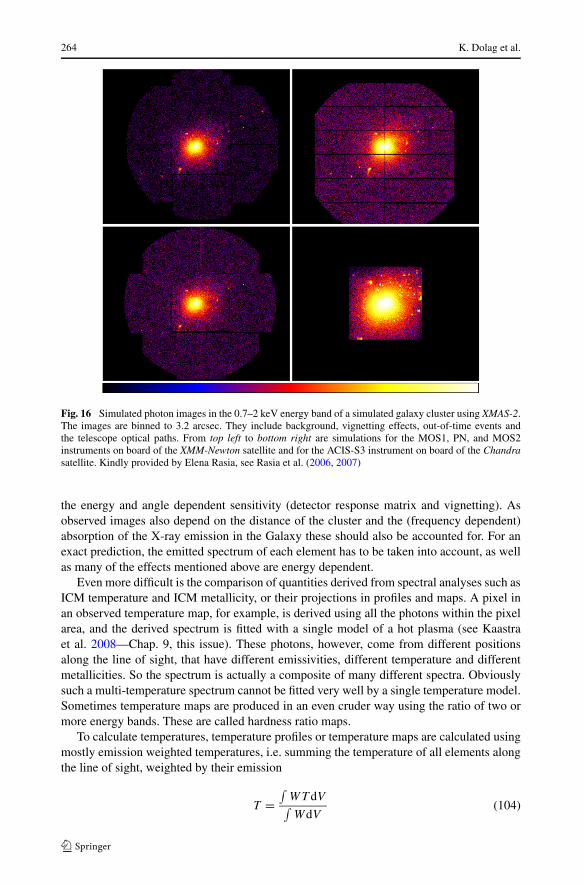
264 K. Dolag et al.

Fig. 16 Simulated photon images in the 0.7–2 keV energy band of a simulated galaxy cluster using XMAS-2.The images are binned to 3.2 arcsec. They include background, vignetting effects, out-of-time events andthe telescope optical paths. From top left to bottom right are simulations for the MOS1, PN, and MOS2instruments on board of the XMM-Newton satellite and for the ACIS-S3 instrument on board of the Chandrasatellite. Kindly provided by Elena Rasia, see Rasia et al. (2006, 2007)

the energy and angle dependent sensitivity (detector response matrix and vignetting). Asobserved images also depend on the distance of the cluster and the (frequency dependent)absorption of the X-ray emission in the Galaxy these should also be accounted for. For anexact prediction, the emitted spectrum of each element has to be taken into account, as wellas many of the effects mentioned above are energy dependent.

Even more difficult is the comparison of quantities derived from spectral analyses such asICM temperature and ICM metallicity, or their projections in profiles and maps. A pixel inan observed temperature map, for example, is derived using all the photons within the pixelarea, and the derived spectrum is fitted with a single model of a hot plasma (see Kaastraet al. 2008—Chap. 9, this issue). These photons, however, come from different positionsalong the line of sight, that have different emissivities, different temperature and differentmetallicities. So the spectrum is actually a composite of many different spectra. Obviouslysuch a multi-temperature spectrum cannot be fitted very well by a single temperature model.Sometimes temperature maps are produced in an even cruder way using the ratio of two ormore energy bands. These are called hardness ratio maps.

To calculate temperatures, temperature profiles or temperature maps are calculated usingmostly emission weighted temperatures, i.e. summing the temperature of all elements alongthe line of sight, weighted by their emission

T =∫

WT dV∫WdV

(104)


with T being the gas temperature and W a weighting factor. Usually W is proportional tothe emissivity of each gas element,

W = �(T )n2 (105)

where �(T ) is the cooling curve and n the gas density.This simple procedure does not of course take into account the shape of the spectra

corresponding to gas of different temperatures. It therefore gives only a rough estimate ofthe actual temperature. With numerical simulations it was investigated how accurate theseemission weighted temperatures are, by comparing them with temperatures obtained by ac-tually adding spectra, so-called spectroscopic temperatures. It was found that the emission-weighted temperatures are systematically higher than the spectroscopic temperatures (Math-iesen and Evrard 2001; Gardini et al. 2004; Mazzotta et al. 2004). To overcome this prob-lem, Mazzotta et al. (2004) suggested an approximation to the spectroscopic temperature,the “spectroscopic-like” temperature Tsl

Tsl =∫

n2T α/T 1/2dV∫n2T α/T 3/2dV

(106)

which yields for α = 0.75 a good estimate of the spectroscopic temperature. In addition thesimulated M–T relation is strongly affected, if the emission-weighted temperature is used(Rasia et al. 2005).

The inhomogeneous temperature and metal distribution was also found to be responsiblealso for inaccurate metallicity measurements. Rasia et al. (2007) studied with numericalsimulations, together with the programme X-MAS2, how well the elements Fe, O, Mg andSi can be measured in clusters of different temperature. They find that Fe and Si are generallymeasurable with good accuracy, while O and Mg can be considerably overestimated in hotclusters. Using simulations and the programme SPEX (see Kaastra et al. 2008—Chap. 9, thisissue) Kapferer et al. (2007) found that due to the metal inhomogeneities the metal mass inclusters is systematically underestimated—in extreme cases by up to a factor of three.

An example of synthetic X-ray observations is shown in Fig. 16. Here XMAS-2 is usedto produce photon images from a simulated galaxy cluster. Shown are simulations for theMOS1, PN, and MOS2 instruments on board the XMM-Newton satellite, and for the ACIS-S3 instrument on board the Chandra satellite. They include instrumental effects like back-ground, vignetting and response for the individual instruments. For more details see Rasiaet al. (2006) and Rasia et al. (2007).

6 Outlook

In the future, the demand on precision in both simulation techniques and captured com-plexity of the physical processes within the simulations will be quite challenging. Recentleading simulations are already extremely difficult to analyse due to their enormous sizeand complexity, and they will surely continue to grow. In fact, the next generation of su-percomputers will grow more in the number of accessible CPUs than on the speedup of theindividual CPUs and this fact will make the analysis of the simulations as challenging asperforming the simulations itself. To keep a comparable level of accuracy, the interpretationof a simulation of the next generation of high precision experiments will need to massivelyinvolve virtual telescopes as described in the previous section. This will increase the need

266 K. Dolag et al.

of involving complex analysis pipelines for “observing” simulations, and might lead to anew branch of virtual observers in the astrophysics community, similar to the already, newformed branch of computational astrophysicists.

Acknowledgements The authors thank ISSI (Bern) for support of the team “Non-virialised X-ray com-ponents in clusters of galaxies”. Special thanks to Volker Springel for helping to improve the manuscriptand providing Fig. 7 to Anna Watts for carefully reading the manuscript, to Martin Obergaulinger for veryhelpful discussions on Eulerian schemes, to Ewald Müller for the lecture notes on the Riemann problem andproviding Fig. 10, to Elena Rasia for providing Fig. 16 and to Umberto Maio for providing Fig. 12. A.D. alsogratefully acknowledges partial support from the PRIN2006 grant “Costituenti fondamentali dell’Universo”of the Italian Ministry of University and Scientific Research and from the INFN grant PD51.

References

T. Abel, P. Anninos, Y. Zhang, M.L. Norman, New Astron. 2, 181 (1997)O. Agertz, B. Moore, J. Stadel et al., Mon. Not. R. Astron. Soc. 380, 963 (2007)E. Athanassoula, A. Bosma, J.-C. Lambert, J. Makino, Mon. Not. R. Astron. Soc. 293, 369 (1998)J.S. Bagla, J. Astrophys. Astron. 23, 185 (2002)J.S. Bagla, S. Ray, New Astron. 8, 665 (2003)D.S. Balsara, J. Comput. Phys. 121, 357 (1995)J.M. Bardeen, J.R. Bond, N. Kaiser, A.S. Szalay, Astrophys. J. 304, 15 (1986)J. Barnes, P. Hut, Nature 324, 446 (1986)E. Bertschinger, COSMICS: Cosmological initial conditions and microwave anisotropy codes. astro-

ph/9506070 (1995)P. Bode, J.P. Ostriker, G. Xu, Astrophys. J. Suppl. Ser. 128, 561 (2000)A. Bonaldi, G. Tormen, K. Dolag, L. Moscardini, Mon. Not. R. Astron. Soc. 378, 1248 (2007)S. Borgani, K. Dolag, G. Murante et al., Mon. Not. R. Astron. Soc. 367, 1641 (2006)S. Borgani, D. Fabjan, L. Tornatore et al., Space Sci. Rev. (2008). doi:10.1007/s11214-008-9322-7G.L. Bryan, M.L. Norman, J.M. Stone, R. Cen, J.P. Ostriker, Comput. Phys. Commun. 89, 149 (1995)R. Cen, Astrophys. J. Suppl. Ser. 78, 341 (1992)S.C. Chapra, R.P. Canale, Numerical Methods for Engineers: With Programming and Software Applications

(McGraw–Hill, New York, 1997)P. Colella, H.M. Glaz, J. Comput. Phys. 59, 264 (1985)P. Colella, P.R. Woodward, J. Comput. Phys. 54, 174 (1984)H.M.P. Couchman, Astrophys. J. 368, L23 (1991)H.M.P. Couchman, P.A. Thomas, F.R. Pearce, Astrophys. J. 452, 797 (1995)R. Courant, K.O. Friedrichs, Supersonic Flow and Shock Waves (Interscience, New York, 1948)W. Dehnen, Astrophys. J. 536, L39 (2000)K. Dolag, M. Jubelgas, V. Springel, S. Borgani, E. Rasia, Astrophys. J. Lett. 606, L97 (2004)K. Dolag, F. Vazza, G. Brunetti, G. Tormen, Mon. Not. R. Astron. Soc. 364, 753 (2005)K. Dolag, A.M. Bykov, A. Diaferio, Space Sci. Rev. (2008). doi:10.1007/s11214-008-9319-2G. Efstathiou, M. Davis, S.D.M. White, C.S. Frenk, Astrophys. J. Suppl. Ser. 57, 241 (1985)B. Einfeldt, SIAM J. Numer. Anal. 25, 294 (1988)B. Einfeldt, P.L. Roe, C.D. Munz, B. Sjogreen, J. Comput. Phys. 92, 273 (1991)S. Ettori, K. Dolag, S. Borgani, G. Murante, Mon. Not. R. Astron. Soc. 365, 1021 (2006)A.E. Evrard, Mon. Not. R. Astron. Soc. 235, 911 (1988)A.E. Evrard, T.J. MacFarland, H.M.P. Couchman et al., Astrophys. J. 573, 7 (2002)L.-L. Feng, C.-W. Shu, M. Zhang, Astrophys. J. 612, 1 (2004)C.S. Frenk, S.D.M. White, P. Bode et al., Astrophys. J. 525, 554 (1999)B. Fryxell, K. Olson, P. Ricker et al., Astrophys. J. Suppl. Ser. 131, 273 (2000)T. Fukushige, T. Ito, J. Makino et al., Publ. Astron. Soc. Jpn. 43, 841 (1991)D. Galli, F. Palla, Astron. Astrophys. 335, 403 (1998)A. Gardini, E. Rasia, P. Mazzotta et al., Mon. Not. R. Astron. Soc. 351, 505 (2004)R.A. Gingold, J.J. Monaghan, Mon. Not. R. Astron. Soc. 181, 375 (1977)F. Haardt, P. Madau, Astrophys. J. 461, 20 (1996)A. Harten, J. Comput. Phys. 49, 357 (1983)A. Harten, P.D. Lax, B. van Leer, SIAM Rev. 25, 35 (1983)A. Harten, B. Engquist, S. Osher, S.R. Chakravarthy, J. Comput. Phys. 71, 231 (1987)

http://dx.doi.org/10.1007/s11214-008-9322-7

http://dx.doi.org/10.1007/s11214-008-9319-2


K. Heitmann, Z. Lukic, P. Fasel et al., astro-ph/0706.1270 (2007). Report LA-UR-07-1953L. Hernquist, Astrophys. J. 404, 717 (1993)L. Hernquist, N. Katz, Astrophys. J. Suppl. Ser. 70, 419 (1989)R.W. Hockney, J.W. Eastwood, Computer Simulation Using Particles (Hilger, Bristol, 1988)P. Hut, J. Makino, S. McMillan, Astrophys. J. 443, L93 (1995)I.T. Iliev, B. Ciardi, M.A. Alvarez et al., Mon. Not. R. Astron. Soc. 371, 1057 (2006)T. Ito, J. Makino, T. Fukushige et al., Publ. Astron. Soc. Jpn. 45, 339 (1993)G.-S. Jiang, C.-W. Shu, J. Comput. Phys. 126, 202 (1996)M. Jubelgas, V. Springel, K. Dolag, Mon. Not. R. Astron. Soc. 351, 423 (2004)J.S. Kaastra, F.B.S. Paerels, F. Durret, S. Schindler, P. Richter, Space Sci. Rev. (2008). doi:10.1007/

s11214-008-9310H. Kang, J.P. Ostriker, R. Cen et al., Astrophys. J. 430, 83 (1994)W. Kapferer, T. Kronberger, J. Weratschnig, S. Schindler, Astron. Astrophys. 472, 757 (2007)N. Katz, D.H. Weinberg, L. Hernquist, Astrophys. J. Suppl. Ser. 105, 19 (1996)A. Kawai, T. Fukushige, J. Makino, M. Taiji, Publ. Astron. Soc. Jpn. 52, 659 (2000)A. Kravtsov, in APS Meeting Abstracts (2002). http://flux.aps.org/meetings/YR02/APR02/baps/abs/S820004.

htmlA.V. Kravtsov, A.A. Klypin, A.M. Khokhlov, Astrophys. J. Suppl. Ser. 111, 73 (1997)A.V. Kravtsov, D. Nagai, A.A. Vikhlinin, Astrophys. J. 625, 588 (2005)R. LeVeque, Finite Volume Methods for Hyperbolic Problems. Cambridge Texts in Applied Mathematics

(Cambridge University Press, Cambridge, 2002)D. Levy, G. Puppo, G. Russo, Berkeley CPAM 762 (1999). arXiv:math/9911089S. Li, J. Comput. Phys. 203, 344 (2005)S. Li, H. Li, R. Cen, Astrophys. J. Suppl. Ser. 174, 1–12 (2008). astro-ph/0611863L.B. Lucy, Astron. J. 82, 1013 (1977)U. Maio, K. Dolag, B. Ciardi, L. Tornatore, Mon. Not. R. Astron. Soc. 379, 963 (2007)J. Makino, Publ. Astron. Soc. Jpn. 43, 621 (1991)B.F. Mathiesen, A.E. Evrard, Astrophys. J. 546, 100 (2001)P. Mazzotta, E. Rasia, L. Moscardini, G. Tormen, Mon. Not. R. Astron. Soc. 354, 10 (2004)M. Meneghetti, P. Melchior, A. Grazian et al., Astron. Astrophys. (2008, in press). astro-ph/0711.3418J.J. Monaghan, Annu. Rev. Astron. Astrophys. 30, 543 (1992)J.J. Monaghan, J. Comput. Phys. 136, 298 (1997)J.J. Monaghan, R.A. Gingold, J. Comput. Phys. 52, 374 (1983)J.P. Morris, J.J. Monaghan, J. Comput. Phys. 136, 41 (1997)J.F. Navarro, S.D.M. White, Mon. Not. R. Astron. Soc. 265, 271 (1993)B.W. O’Shea, K. Nagamine, V. Springel, L. Hernquist, M.L. Norman, Astrophys. J. Suppl. Ser. 160, 1 (2005)J.M. Owen, J.V. Villumsen, P.R. Shapiro, H. Martel, Astrophys. J. Suppl. Ser. 116, 155 (1998)P.J.E. Peebles, The Large-Scale Structure of the Universe (Princeton University Press, Princeton, 1980)U.-L. Pen, Astrophys. J. Suppl. Ser. 115, 19 (1998)K.G. Powell, P.L. Roe, T.J. Linde, T.I. Gombosi, D.L. de Zeeuw, J. Comput. Phys. 154, 284 (1999)C. Power, J.F. Navarro, A. Jenkins et al., Mon. Not. R. Astron. Soc. 338, 14 (2003)W.H. Press, S.A. Teukolsky, W.T. Vetterling, B.P. Flannery, Numerical Recipes in FORTRAN. The Art of

Scientific Computing, 2nd edn. (Cambridge University Press, Cambridge, 1992)T. Quinn, N. Katz, J. Stadel, G. Lake, Astrophys. J. (1997). Submitted but not published, astro-ph/9710043E. Rasia, P. Mazzotta, S. Borgani et al., Astrophys. J. 618, L1 (2005)E. Rasia, S. Ettori, L. Moscardini et al., Mon. Not. R. Astron. Soc. 369, 2013 (2006)E. Rasia, P. Mazzotta, H. Bourdin et al., Astrophys. J. (2007, in press). astro-ph/0707.2614P.M. Ricker, S. Dodelson, D.Q. Lamb, Astrophys. J. 536, 122 (2000)D. Ryu, J.P. Ostriker, H. Kang, R. Cen, Astrophys. J. 414, 1 (1993)H.-Y. Schive, C.-H. Chien, S.-K. Wong, Y.-C. Tsai, T. Chiueh, New Astron. (2007, in press). astro-

ph/0707.2991C.-W. Shu, in Advanced Numerical Approximate of Nonlinear Hyperbolic Equations, ed. by A. Quarteroni.

Lecture Notes in Mathematics, vol. 1697 (Springer, Berlin, 1998), p. 285D. Sijacki, V. Springel, T. di Matteo, L. Hernquist, Mon. Not. R. Astron. Soc. 380, 877 (2007)B.W. Silverman, Density Estimation for Statistics and Data Analysis. Monographs on Statistics and Applied

Probability (Chapman & Hall, London, 1986)V. Springel, Mon. Not. R. Astron. Soc. 364, 1105 (2005)V. Springel, L. Hernquist, Mon. Not. R. Astron. Soc. 333, 649 (2002)V. Springel, L. Hernquist, Mon. Not. R. Astron. Soc. 339, 289 (2003)V. Springel, M. White, L. Hernquist, Astrophys. J. 549, 681 (2001a)V. Springel, N. Yoshida, S.D.M. White, New Astron. 6, 79 (2001b)

http://dx.doi.org/10.1007/s11214-008-9310

http://dx.doi.org/10.1007/s11214-008-9310

268 K. Dolag et al.

M. Steinmetz, Mon. Not. R. Astron. Soc. 278, 1005 (1996a)M. Steinmetz, in IAU Symp. 171: New Light on Galaxy Evolution (1996b), p. 259F. Stoehr, S.D.M. White, V. Springel, G. Tormen, N. Yoshida, Mon. Not. R. Astron. Soc. 345, 1313 (2003)J.M. Stone, M.L. Norman, Astrophys. J. Suppl. Ser. 80, 753 (1992)R.S. Sutherland, M.A. Dopita, Astrophys. J. Suppl. Ser. 88, 253 (1993)G. Tormen, F.R. Bouchet, S.D.M. White, Mon. Not. R. Astron. Soc. 286, 865 (1997)S.D.M. White, in Cosmology and Large Scale Structure, ed. by R. Schaeffer, J. Silk, M. Spiro, J. Zinn-Justin

(1996) p. 349G. Xu, Astrophys. J. Suppl. Ser. 98, 355 (1995)Y.B. Zel’dovich, Astron. Astrophys. 5, 84 (1970)

simulation techniques for cosmological simulations

Documents