simulation of the heater test room defined by en...

i

SIMULATION OF THE HEATER TEST ROOM DEFINED BY EN 442 STANDARD AND VIRTUAL TESTING OF DIFFERENT TYPE OF HEATERS

A Thesis Submitted to the Graduate School of Engineering and Sciences of

İzmir Institute of Technology in Partial Fulfillment of the Requirements for the Degree of

DOCTOR OF PHILOSOPHY

in Mechanical Engineering

by Abdullah Berkan ERDOĞMUŞ

January 2011

İZMİR

ii

We approve the thesis of Abdullah Berkan ERDOĞMUŞ __________________________________ Prof. Dr. Zafer İLKEN Supervisor __________________________________ Prof. Dr. Barış ÖZERDEM Co-Supervisor __________________________________ Assoc. Prof. Dr. Selahattin YILMAZ Committee Member __________________________________ Assoc. Prof. Dr. Moghtada MOBEDİ Committee Member __________________________________ Assist. Prof.Dr. Hüseyin GÜNERHAN Committee Member __________________________________ Assist. Prof. Dr. Ünver ÖZKOL Committee Member 07 January 2011 __________________________ ___________________________ Prof. Dr. Metin TANOĞLU Prof. Dr. Durmuş Ali DEMİR Head of the Department of Dean of the Graduate School of Mechanical Engineering Engineering and Sciences

iii

ACKNOWLEDGMENTS

First of all, I would like to express my sincere gratitude and deepest respect to

my supervisor Prof. Dr. Zafer İLKEN for his support throughout PhD program.

Working under the supervision of Prof. Dr. Zafer İLKEN is a great honor for me. I am

heartily thankful to my co-supervisor, Prof. Dr. Barış ÖZERDEM, whose constant

encouragement; friendly personality enabled me to complete this study. He gave me

invaluable recommendations throughout my academic studies.

I would like to thank Assoc. Prof. Dr. Moghtada MOBEDİ for giving insightful

feedback to improve the contents of this study. He helped me to understand

fundamental concepts and shows me applying different approaches to accomplish a

research problem. I would like to thank Assoc. Prof. Dr. Selahattin YILMAZ for giving

valuable recommendations. His constructive comments led to substantial improvements

of the study. I would like to thank thesis committee members. Their suggestions helped

me to clarify my ideas and strengthen my research.

It is my great pleasure to thank the management board of ELBA Inc. for

permission to use radiator test room and collaboration. Their supports to scientific

works are admirable. I am extremely thankful to Okan EROĞLU, the production

manager of ELBA Inc., and Serdar ELÇE. Their endless supports were unforgettable. I

would like to show my gratitude to Cihan ŞAHİN and Ümit AYANDIN. Their

experiences shortened the test period and accelerate this study.

I would like to thank İhsan ÖZSOY, Dr. Ali M. ÇOLAKOĞLU, and Birol

ERENTURK for giving a chance to deal with related problems in ASELSAN Inc.

Researches increased my experiences in computational heat transfer and fluid dynamics

applications. It is a pleasure to thank my colleagues Erkin GEZGİN, A. Cem

GÖZÜKARA, Mustafa OCAK, A. Levent AVŞAR and Murat ŞAHİN for

understanding and contributions in various stages of this study. I would like to express

my gratitude to my other colleagues working in MGEO Division of ASELSAN Inc.,

sincere and scientific atmosphere and their motivations increased my concentration. I

am also grateful to Emre OZTURK and ANOVA Company for giving supports

whenever I required.

Finally, I would like to thank my family for their endless and complimentary

support especially in distressful times.

iv

ABSTRACT

SIMULATION OF THE HEATER TEST ROOM DEFINED BY EN 442 STANDARD AND VIRTUAL TESTING OF DIFFERENT TYPE OF

HEATERS

Heat outputs of radiators are determined experimentally in specific conditions.

Many standards have been developed to identify test conditions. EN442 standard

specifies test room properties, temperature measurements and heat output calculations

for radiators. In this study, the heat dissipation capabilities of three different panel

radiators were determined by using numerical methods. The height and length of the

tested radiators were 600 mm and 1000 mm, respectively. An experimental study was

conducted in the standard test room in order to determine boundary conditions for

computational study and verify numerical results. Tests were carried out in three

different operating conditions. Twelve measurements were performed in each condition

when test room reached steady state. Turbulent typed air flow in the test room and water

flow inside the tested radiators were simulated. Temperature and velocity contours in

virtual test room are also investigated in this study. Non uniform temperature

distribution on the front surface of tested radiators was observed. It is seen that the

symmetricity in velocity contours is distorted by using more complex radiator models

and increasing excess temperature. The difference between experimental and

computational heat output fluctuates between 0.4% and 13.6% for the simplest model,

3.4% and 11.1% for the second radiator, 4.5% and 12.9% for most complicated model

investigated in this study. Good results are obtained for the excess temperature of 50oC

and 60oC. For the lowest excess temperature, results are also in acceptable range. The

study shows that computational methods can be applicable in the design of new heater

types.

v

ÖZET

EN 442 STANDARDI İLE TANIMLANMIŞ ISITICI TEST ODASININ SİMULASYONU VE DEĞİŞİK TİPTEKİ

ISITICILARIN SANAL TESTLERİ

Radyatörlerin ısı yayma kapasiteleri belirli koşullar için deneysel çalışmalar ile

belirlenir. Test koşullarını belirlemek için birçok standart geliştirilmiştir. EN 442

standardı ile radyatörler için test odasının özellikleri, sıcaklık ölçümleri ve ısı yayma

kapasitelerini hesaplanma detayları tanımlanmıştır. Test edilen radyatörlerin yükseklik

ve uzunlukları sırayla 600 mm ve 1000 mm dir. Bu çalışmada üç farklı panel radyatörün

ısı yayma kapasitesi sayısal yollarla hesaplanmıştır. Nümerik çalışmada kullanılacak

sınır şartlarını belirlemek ve nümerik yollarla elde edilen sonuçları doğrulamak için

deneysel bir çalışma gerçekleştirilmiştir. Testler üç farklı aşırı sıcaklık çalışma şartına

dayanarak yapılmıştır. Her bir aşırı sıcaklık testi için kararlı hal durumuna erişildiğinde

oniki sıcaklık ölçümü yapılmıştır. Türbülanslı hava akışı ve radyatör içindeki suyun

akışı birlikte simüle edilmiştir. Bu çalışmada aynı zamanda test odası içindeki sıcaklık

ve hız dağılımlarıda incelenmiştir. Test edilen radyatör yüzeylerindeki sıcaklığın her

bölgede aynı olmadığı gözlenmiştir. Karmaşık radyatör modellerinde ve yüksek aşırı

sıcaklıklarda çizdirilen hız eğrilerinin radyatör eksenine simetrikliklerinin bozulduğu

görülmüştür. Deneysel ve nümerik yollarla hesaplanan ısı yayma kapasiteleri arasındaki

farkın radyatör I için %0.4 ile %13.6 arasında, radyatör II için %3.4 ile %11.1 arasında,

radyatör III için %4.5% ile %12.9 değiştiği bulunmuştur. 50oC ve 60oC aşırı sıcaklıklar

için nümerik yollarla elde edilen sonuçların oldukça iyi, 30oC aşırı sıcaklıkta ise kabul

edilebilir bir aralıkta olduğu değerlendirilmiştir. Bu çalışma yeni ısıtıcı tiplerinin

geliştirilmesinde sayısal metotların kullanımının uygulanabilir olduğunu

göstermektedir.

vi

TABLE OF CONTENTS

LIST OF FIGURES .......................................................................................................... x

LIST OF TABLES......................................................................................................... xiv

LIST OF SYMBOLS....................................................................................................xvii

CHAPTER 1. INTRODUCTION ..................................................................................... 1

1.1. Central Heating ....................................................................................... 1

1.2. Heating Devices in Central Heating Systems ......................................... 2

1.3. Types of Radiators .................................................................................. 3

1.3.1. Stainless Steel Radiators................................................................... 4

1.3.1.1. Panel Radiators........................................................................ 6

1.3.1.1.1. Single Panel Radiators................................................ 7

1.3.1.1.2. Double Panel Radiators .............................................. 7

1.3.1.1.3. Panel Radiators with Extended Surfaces.................... 8

1.4. Heat Transfer from Radiators ................................................................. 9

1.5. Heat Requirement of Buildings ............................................................ 10

1.6. Heat Output of Radiators ...................................................................... 10

1.7. Unique Contribution and Parts of the Study ......................................... 12

CHAPTER 2. THEORY................................................................................................. 14

2.1. Convective Heat Transfer .................................................................... 14

2.2. Radiative Heat Transfer ....................................................................... 17

2.3. Flow Types and Properties................................................................... 18

2.4. Governing Equations ........................................................................... 19

2.4.1. Continuity Equation ....................................................................... 20

2.4.2. Momentum Equations.................................................................... 20

2.4.3. Energy Equation............................................................................. 22

2.5. Boussinessq Approximation ................................................................. 23

2.6. Turbulent Flows .................................................................................... 24

2.6.1. Continuity Equation for Turbulent Flows....................................... 25

vii

2.6.2. Reynolds Average Navier Stokes Equations .................................. 25

2.7. Boussinesq Hypothesis ......................................................................... 27

2.8. Turbulence Modeling............................................................................ 27

2.8.1. Two Equation Turbulence Models.................................................. 28

2.8.1.1. The k- ε Turbulence Model.................................................... 28

2.8.1.1.1. Standard k- ε Turbulence Model................................ 29

2.8.1.1.2. Realizable k- ε Turbulence Model ............................. 30

2.8.2. Energy Equation in the k- ε Models................................................ 32

2.9. Modeling Near Wall Regions ............................................................... 32

2.10. Radiative Transfer Equation .............................................................. 35

2.10.1. The Discrete Ordinates Radiation Model ................................... 37

2.11. Basics of Computational Fluid Dynamics .......................................... 37

2.11.1. Geometry Preparation ................................................................. 38

2.11.2. Mesh Generation......................................................................... 39

2.11.3. Selection of Numerical Method .................................................. 41

2.11.3.1. Finite Difference Method................................................. 42

2.11.3.2. Finite Volume Method..................................................... 44

2.11.4. Identification of Flow Conditions and Properties....................... 46

2.11.5. Defining Initial and Boundary Conditions.................................. 47

2.11.6. Solver Selection .......................................................................... 49

2.12.7. Selection of Numerical Scheme.................................................. 54

2.11.8. Under-Relaxation Factor Settings............................................... 56

2.11.9. Termination Criteria and Convergence....................................... 57

2.11.10. CFD Errors................................................................................ 59

2.11.11. Post-Processing ......................................................................... 59

CHAPTER 3. STANDARDS ON DETERMINATION OF RADIATORS HEAT

OUTPUT ................................................................................................. 60

3.1. Previous Standards................................................................................ 60

3.2. European Standard EN 442 Part 2 ........................................................ 60

3.2.1. The Characteristics of Heater Test Room Specified in

EN 442 ........................................................................................... 61

3.2.2. The Determination of Standard Characteristic Equation and

EN 442 Heat Output ..................................................................... 62

viii

CHAPTER 4. LITERATURE REVIEW........................................................................ 66

4.1. Studies on Two Dimensional Heat Transfer and Fluid Flows............. 67

4.2. Studies on Three Dimensional Heat Transfer and Fluid Flows........... 80

CHAPTER 5. EXPERIMENTAL STUDY .................................................................... 85

5.1. Test Procedure ...................................................................................... 85

5.2. Measured Values................................................................................... 88

5.3. Calculation of Experimental Heat Outputs ........................................... 92

5.4. Calculation of EN 442 Standard Heat Outputs ..................................... 95

CHAPTER 6. VERIFICATION OF TWO DIMENSIONAL NATURAL

CONVECTION IN CAVITY ................................................................. 97

6.1. Two Dimensional Differential Heating ............................................... 97

CHAPTER 7. BOUNDARY CONDITIONS AND COMPUTATIONAL DETAILS 118

7.1. Pre-Analysis....................................................................................... 118

7.1.1. Natural Convection in Cavity with Three Cold and One

Hot Sides...................................................................................... 118

7.1.2. Cavity with Three Cold and One Partially Heated Sides............. 121

7.1.3. Natural Convection in the Cavity with Internal Heated Body..... 123

7.1.4. Natural Convection in a Three Dimensional Enclosure with an

Internal Heated Body................................................................... 125

7.2. CFD Analysis of Tested Radiators ..................................................... 130

7.2.1. ICEPAK Models for Tested Radiators ......................................... 130

7.2.2 Mesh Details .................................................................................. 132

7.2.3. Boundary Conditions .................................................................... 135

7.2.4. Assumptions and Solver Settings.................................................. 137

7.2.5. Convergence Criteria .................................................................... 138

7.2.6. Comparison of Results.................................................................. 140

CHAPTER 8. RESULTS AND DISCUSSION............................................................ 141

8.1. CFD Results for Radiator I ................................................................ 141

8.2. CFD Results for Radiator II ............................................................... 148

8.3. CFD Results for Radiator III.............................................................. 155

ix

CHAPTER 9. CONCLUSION ..................................................................................... 162

REFERENCES ............................................................................................................. 166

APPENDICES

APPENDIX A. TABLES FROM EN 442 STANDARD ............................................. 170

APPENDIX B . MEASURED DATA........................................................................... 171

APPENDIX C. ADDITIONAL CODE USED IN FLUENT ....................................... 180

x

LIST OF FIGURES

Figure Page

Figure 1.1. Different connection styles of radiators....................................................... 3

Figure 1.2. Sectional view from panel radiators. ........................................................... 6

Figure 1.3. Schematic view of single and double panel radiators.................................. 7

Figure 1.4. Schematic view of different type of panel radiators which include fins. .... 9

Figure 2.1. Cell shapes used in 2D geometries (a) Triangle (b) Quadrilateral ............ 39

Figure 2.2. Cells used in 3D geometries (a) Cube (b) Rectangular Prism (c)

Tetrahedron (d) Hexahedron (e) Prism (f) Pyramid .................................. 40

Figure 2.3. Discrete grid points for finite difference method ...................................... 42

Figure 2.4. A finite volume in one dimension. ............................................................ 45

Figure 2.5. Segregated solution procedure................................................................... 49

Figure 2.6. Coupled solution procedure....................................................................... 49

Figure 2.7. Unsteady solution procedure ..................................................................... 50

Figure 2.8. Overwiew of the density-based solution methods..................................... 50

Figure 2.9. Overwiew of the pressure-based solution methods. .................................. 51

Figure 2.10. SIMPLE algorithm in steady state............................................................. 53

Figure 2.11. SIMPLE algorithm in transient solutions .................................................. 53

Figure 2.12. Upwind, central differencing, power law and quick schemes. .................. 55

Figure 3.1. Water channels in test room panels. .......................................................... 61

Figure 3.2. Cooling of test room panels....................................................................... 62

Figure 3.3. Schematic view of test set up when weighting method is applied. ........... 64

Figure 4.1. Temperature contours (isotherms) at different Rayleigh numbers............ 69

Figure 4.2. Stream functions at different Rayleigh numbers. ...................................... 70

Figure 4.3. Experimental set up performed by Tian and Karaannis. ........................... 73

Figure 4.4. The Principle of a laser doppler anemometer. ........................................... 74

Figure 4.5. Local Nusselt numbers on vertical and horizontal walls........................... 75

Figure 4.6. Wall temperatures found by Ampofo and Karaannis. ............................... 76

Figure 4.7. Vertical velocity profile near the hot wall. ................................................ 77

Figure 4.8. Experimental set up performed by Beck. .................................................. 78

Figure 4.9. Configurations investigated by Beck......................................................... 79

Figure 4.10. Velocity profiles with no, one and two sheets in the gap. ......................... 80

xi

Figure 4.11. Wall temperatures of the fully coupled radiator models. .......................... 82

Figure 5.1. View from tested radiators. ....................................................................... 85

Figure 5.2. Placement of a radiator during a test procedure. ....................................... 86

Figure 5.3. Measuring of air temperature inside the test room. ................................... 86

Figure 5.4. Thermal camera view from the flexible connections. ............................... 87

Figure 5.5. Flow rates in tests of radiator I. ................................................................. 89

Figure 5.6. Reference air temperatures in tests of radiator I........................................ 89

Figure 5.7. Mean water temperatures in tests of radiator I. ......................................... 89

Figure 5.8. Flow rates in tests of radiator II................................................................. 90

Figure 5.9. Reference air temperatures in tests of radiator II. ..................................... 90

Figure 5.10. Mean water temperatures in tests of radiator II. ........................................ 90

Figure 5.11. Flow rates in tests of radiator III. .............................................................. 91

Figure 5.12. Reference air temperatures in tests of radiator III. .................................... 91

Figure 5.13. Mean water temperatures in tests of radiator III........................................ 91

Figure 5.14. Temperature distributions on the front surface of radiator I. .................... 92

Figure 5.15. Experimental heat outputs of radiator I (W).............................................. 93

Figure 5.16. Experimental heat outputs of radiator II (W). ........................................... 93

Figure 5.17. Experimental heat outputs of radiator III (W). .......................................... 93

Figure 5.18. Enhancement in the heat transfer rates when radiator II is compared

with radiator I (in percantage). .................................................................. 94

Figure 5.19. Enhancement in the heat transfer rates when radiator III is compared

with radiator I (in percantage). .................................................................. 94

Figure 6.1. Contours obtained for Ra=102. ................................................................ 100




Figure 6.7. Change in middle point temperature for Ra=108..................................... 106


Figure 6.9. Velocity vectors for Ra=108. ................................................................... 107

Figure 6.10. Contours obtained for Ra=1010................................................................ 108

Figure 7.1. Contours obtained for the cavity whose three side is cold and the

other side is hot........................................................................................ 120

Figure 7.2. Contours obtained for the cavity which has three cold and one partially

heated side. .............................................................................................. 122

xii

Figure 7.3. The schematic view of cavity with internal heated body. ....................... 123

Figure 7.4. Contours for cavity with internal heated body. ....................................... 124

Figure 7.5. The sectional view of grid created for 3D domain (Grid II). .................. 126

Figure 7.6. The temperature contour (oC) at vertical plane (II-II) whose normal is

in the z direction (Grid II)........................................................................ 126

Figure 7.7. The velocity contour (oC) at vertical plane (II-II) whose normal is in

the z direction (Grid II)............................................................................ 127

Figure 7.8. The temperature contour (oC) at vertical plane (III-III) whose normal

is in the x direction (Grid II).................................................................... 127

Figure 7.9. The temperature contour at vertical plane (I-I) whose normal is in

the x direction (Grid II and x=2.398) ...................................................... 128

Figure 7.10. Y velocity contours at vertical plane (I-I) whose normal is in x

direction (Grid II). ................................................................................... 128

Figure 7.11. Velocity vectors (Grid II). ....................................................................... 129

Figure 7.12. ICEPAK models of tested radiators......................................................... 131

Figure 7.13. Details of CFD model of single panel. .................................................... 131

Figure 7.14. Comparison of real and CFD models. ..................................................... 132

Figure 7.15. A cross sectional view of grid created in the virtual test room which

includes radiator I. ................................................................................... 133

Figure 7.16. The grid density around radiator I. .......................................................... 133

Figure 7.17. A cross sectional view of grid created for the test room includes

radiator II. ................................................................................................ 134

Figure 7.18. The grid density around radiator II.......................................................... 134

Figure 7.19. A cross sectional view of grid created for the test room includes

radiator III................................................................................................ 135

Figure 7.20. The grid density around radiator III. ....................................................... 135

Figure 7.21. Residuals in the final CFD run for radiator II (Case 1). .......................... 139

Figure 7.22. Reference point temperature in the final CFD run for radiator II

(Case 1).................................................................................................... 139

Figure 7.23. Air velocities in the final CFD run for radiator II (Case 1). .................... 139

Figure 8.1. Temperature distribution on vertical mid plane of radiator I

(z=0.4559 m). .......................................................................................... 142

Figure 8.2. Temperature distributions at three different horizontal cross sections

of radiator I. ............................................................................................. 143

xiii

Figure 8.3. Temperature contours on the vertical mid plane of virtual test room

whose normal is in z direction (z=2.405 m). ........................................... 144

Figure 8.4. Temperature contours on the vertical mid plane of virtual test room

whose normal is in x direction (x=2.398 m)............................................ 145

Figure 8.5. Temperature contours on the horizontal mid plane of virtual test room

whose normal is in y direction (y=1.867 m)............................................ 146

Figure 8.6. Velocity contours on the vertical mid plane of virtual test room whose

normal is in z direction (z=2.405 m). ...................................................... 147

Figure 8.7. Temperature distribution on vertical mid plane of panel used in

radiator II. ................................................................................................ 149

Figure 8.8. Temperature distribution on a horizontal cross section of radiator II. .... 150

Figure 8.9. Temperature contours on the vertical mid plane whose normal is in z

direction (z=2.405 m). ............................................................................. 151

Figure 8.10. Temperature contours on the vertical mid plane whose normal is in x

direction (x=2.398 m). ............................................................................. 152

Figure 8.11. Velocity contours on the vertical mid plane whose normal is in z

direction (z=2.405 m). ............................................................................. 153

Figure 8.12. Path lines for the air motion in virtual test of radiator II......................... 154

Figure 8.13. Pathlines for the air motion in virtual test of radiator III......................... 155

Figure 8.14. Temperature distribution on radiator III in case 1................................... 156



Figure 8.17. Velocity contours on the vertical mid plane whose normal is in z

direction (z=2.405 m). ............................................................................. 159

Figure 8.18. Temperature contours on the vertical mid plane whose normal is in z

direction (z=2.405 m). ............................................................................. 160

xiv

LIST OF TABLES

Table Page

Table 1.1. Proportion of heat emitted as radiation and convection (in an

isothermal cooled surface-enclosure). ......................................................10

Table 1.2. Factors affect the heat output of radiators. ................................................11

Table 2.1. The ratio of the emissivity in accordance with surface

characteristics.............................................................................................18

Table 2.2. Default under relaxation factors in FLUENT and ICEPAK......................57

Table 4.1. Results of simulation performed by Gritzki for the first radiator

model. ........................................................................................................83

Table 4.2. Results of simulation performed by Gritzki for the second radiator

model. ........................................................................................................83

Table 5.1. Mean experimental heat outputs (Φexp) of investigated

radiators(W). ..............................................................................................95

Table 5.2. The radiated heat output factor (Sk), the exponent np and test

pressure for investigated radiators. ............................................................95

Table 5.3. Coefficients used in Equation (3.7) and (3.8) for tested radiators. ............95

Table 5.4. Standard characteristic equations for tested radiators................................96

Table 5.5. EN 442 heat outputs (Φ) of tested radiators (W). ......................................96

Table 5.6. Comparison of experimental and EN 442 heat outputs of tested

radiators in three cases (in percentage)......................................................96

Table 6.1. Details about two dimensional domains in investigated Rayleigh

numbers......................................................................................................98

Table 6.2. Coefficients used for the calculation of Rayleigh numbers. ......................98

Table 6.3. Air properties in two dimensional computational runs..............................98

Table 6.4. Discretization scheme employed in the computational runs of two

dimensional problems. ...............................................................................99

Table 6.5. Heat transfer rates and mean Nusselt number on hot and cold walls

for different number of elements and Ra=102 ...........................................99


for different number of elements and Ra=103. ........................................100

xv


for different number of elements and Ra=104 .........................................101


for different number of elements and Ra=105 .........................................102


for different number of elements and Ra=106. ........................................103

Table 6.10. Heat transfer rates and average Nusselt number on hot and cold

walls for different number of elements and Ra=107. ...............................104

Table 6.11. Comparison of the predicted mean Nusselt number on the hot or

cold walls of a cavity ...............................................................................105

Table 6.12. Total heat transfer rates and mean Nusselt number on hot and cold

walls for Ra=108. .....................................................................................106

Table 6.13. Total heat transfer rates and mean Nusselt number on hot and cold

walls for Ra=1010. ....................................................................................108

Table 6.14. Total heat transfer rates on hot and cold walls for different number

of cells (W). .............................................................................................111

Table 7.1. Total heat transfer rates from the walls and reference temperatures

in different number of elements for two dimensional cavity which

has three cold and one hot sides (W). ......................................................119

Table 7.2. Total heat transfer rates (W) from the walls and reference

temperatures for two dimensional domain which has three cold and

one partially heated side. .........................................................................121

Table 7.3. Total heat transfer rates from the walls (W) and reference

temperatures for cavity with internal heated body..................................123

Table 7.4. Number of elements in two different grid structures generated for

3D enclosure with internal body..............................................................126

Table 7.5. Total heat transfer rates in different grid structures.................................129

Table 7.6. Mesh details for Radiator I. .....................................................................132

Table 7.7. Mesh details for three cases of Radiator II. .............................................134

Table 7.8. Mesh details for three cases and Radiator III. .........................................135

Table 7.9. Boundary conditions at radiator inlet.......................................................136

Table 7.10. Boundary conditions for the walls of virtual tests room (except

wall behind tested radiators) ...................................................................137

xvi

Table 8.1. Computational heat outputs of radiator I in different grid

structures (W). .........................................................................................148

Table 8.2. Compared heat outputs for radiator I (W). ..............................................148

Table 8.3. Computational heat outputs (W) of radiator II in two different grid

structures..................................................................................................154

Table 8.4. Compared heat outputs for radiator II......................................................154

Table 8.5. Computational heat outputs of radiator III in two different grid

structures (W). .........................................................................................161

Table 8.6. Experimental heat outputs of radiator III (W). ........................................161

Table 8.7. Comparison of heat outputs of tested radiators. ......................................161

xvii

LIST OF SYMBOLS

a :Absorption coefficient

ap :Coefficient

anb :Coefficient

C :Specific heat (J/kgK)

Cμ , C2 , C1ε :Constants of turbulence models

ΔTe :Excess temperature

E :Total energy

fx, fy, fz :Source terms

fp :Correction factor

g :Gravitational acceleration

Gb :Generation of turbulence kinetic energy due to buoyancy

Gk :Generation of turbulence kinetic energy due to mean velocity

Gradients

Gr :Grashof number

h :Heat transfer coefficient (W/m2K)

hext :External heat transfer coefficient defined by users

hf :Fluid-side local heat transfer coefficient

i :Enthalpy

I :Radiation intensity

Iλ :Spectral intensity

k :Thermal conductivity (W/mK) or Turbulence kinetic energy

(m2/s2)

kt :Turbulent thermal conductivity

Km :The radiator output constant

L :Length (m)

m :Mass flow rate (kg/s)

n :Refractive index

N :Number of test points

Nu :Nusselt number

p :Static pressure (kPa)

Pe :Peclet number

xviii

Pr :Prandtl number

Q :Heat output (W)

r :Position vector

R :Universal gas constant

Rp :Imbalance

Ra :Rayleigh number

q :Heat flux (W/m2)

qrad :Radiative heat flux

s :Path length for Radiation transport equation

Sh :Source term (volumetric)

Sk :User defines source term or radiated heat output factor

Sε :User-defined source terms.

s :Direction vector

's :Scattering direction vector

T :Temperature (oC or K)

T∞ :Ambient temperature (oC or K)

Trom :Reference air temperature (oC or K)

u, v, w :Velocity components (m/s)

UT :The friction velocity

V :Velocity (m/s) or Volume (m3)

V :Velocity vector

yp :The distance between first cell and wall

YM :Contribution of the fluctuating dilatation incompressible

turbulence to the overall dissipation rate

Greek Symbols

α :Thermal diffusivity or under relaxation factor

β :Expansion coefficient (K-1)

υ :Kinematic viscosity (m2s-1)

∆n :Distance between wall surface and cell center

ε :Energy dissipation rate (m2/s3)

λ :Bulk viscosity coefficient

Ø :Any flow property

xix

φ :Average value of any flow property

φ′ :Instantaneous value of any flow property

μ :Dynamic viscosity (kg/ms)

tμ :Turbulent (eddy) viscosity

ρ :Density (kg/m3)

sσ :Scattering coefficient

г :Diffusion coefficient

τ :Shear stress

(τij)eff :Deviatoric stress tensor

Φ :Dissipation function or corrected (EN 442 standard) heat output

Φ me :Uncorrected heat output (W)

′Ω :Solid angle

Subscripts

c :Cold

comp :Computational

eff :Effective

exp :Experimental

f :Fluid

h :Hot

in :Inlet

out :Outlet

x, y, z :Spatial coordinate directions

o :Operating temperature and standard test conditions.

i,j, k :Suffix notation for x, y and z directions

k :Turbulence kinetic energy

nb :Neighbor cells

s :Solid

w :Water or wall

∞ :Fluid sufficiently far from the hot or cold surfaces.

1

CHAPTER 1

INTRODUCTION

Human beings feel comfortable in buildings in case of specific indoor

temperature; relative humidity and air velocities are maintained. In cold seasons,

thermal comfort is mainly provided with different kind of heating devices in buildings.

Local or joint heat sources are used for heating process. In local heating applications,

spaces are separately heated by using different appliances like electric heaters, radiative

heaters, heat pumps, electrically heated oil-filled radiators and gas-fired or wood fueled

stoves. In central heating applications, joint heat sources are used. Heat generated in one

place is distributed to all spaces of buildings in those applications. Although the

investment cost of a central heating is higher than the cost of local heating, desired or

uniform temperatures can be ensured in whole building and people feel more

comfortable.

1.1. Central Heating

A medium is required in order to carry the heat generated as a result of

combustion of fossil fuel in a joint heat source. Steam or hot water can be utilized as a

primary medium in such applications. When a medium carries the heat, long pipes or

some special devices can be used in order to transfer heat.

Air can also be used as a secondary medium in buildings which have many zones

and different thermal conditions are required like shopping centers, sport centers or

airports. In such systems, air is conditioned first by using previously conditioned water

and then distributed to each zone by insulated ductwork.

Generally, hot water is used as a medium in heating systems of dwellings. In those

systems, tap water is used directly without exposed to any treatment process. Water

treatment can be employed to prevent scaling or corrosion caused by dissolved gasses,

freezing of the water, the growth of mold in complicated heating systems.

2

1.2. Heating Devices in Central Heating Systems

Heat can be discharged to indoor environment by using different equipment from

straight or finned pipes to special heating appliances like radiators. Straight pipes can be

assumed as basic heat exchangers. However heat transfer rates from straight pipes are

very low when they are in contact with stir air. Therefore, the length of piping line

becomes crucial to overcome the required energy.

The heat emitted from the pipe surface can be increased by using finned pipes.

Finned pipes are generally used in convectors or air handling units in which speed of air

is high.

Because of relatively lower investment cost and easy installation, radiators are

widespread heating devices in households when a joint heat source is used. In case

radiators which do not used any external force are utilized in the heating system, air

circulation in indoor environment occurs without using external force.

Radiators are installed to areas such as under windows, along cold walls, or at

doorways where great heat losses occur. Generally, freestanding radiators or radiators in

decorative enclosures are placed symmetrically below the windows or on the external

walls. Different researches show that enclosures affect their effectiveness (Ashrae 2000)

The size of radiator, connection style of supply and return lines, and places can be

different in each project. However radiator dimensions are standard and correct one is

selected from the producers catalogues according to required energy amount. Height of

radiators usually changes between 200 mm and 900 mm while length changes between

400 mm and 3000 mm. The size of a radiator is not important for HVAC engineers

only. Building engineers and architects want to use smaller heaters since smaller ones

use less wall space.

Different supply and return connections can be applied as seen in Figure 1.1

(Radiator Connection 2010). Hot water can enter the radiator from the top and exits

from the bottom of the same side as shown in Figure 1.1 a.) which is one of the

frequently seen connection type. Connection shown in Figure 1.1 b.) is generally

applied when long radiators whose length is 4 or 5 times more than its height are used in

the system. When a radiator is connected from bottom opposite ends as shown in Figure

1.1 c.), the performance of the radiator can decrease depending on the height of the

radiator.

3

Figure 1.1. Different connection styles of radiators.

In Figure 1.1 d.), radiators are connected to circuit constructed from single pipe

line. The surface temperatures of radiators are different from each other in this type of

connection. In the last figure, serial connection is schematically shown. It should be

noted that this connection is not frequently used (Radiator Connection 2010).

1.3. Types of Radiators

Design, material, size and colors of radiators can be different. Comparisons

between different radiators are based on volume and projection area, weight, thermal

inertia, ease of installation, water volume, life, corrosion, aesthetic, security, the

required amount of heating surface, pressure resistance and price. It is possible to

classify radiators according to construction material as cast iron radiators, steel radiators

and aluminum radiators. Panel radiators, panel radiators with extended surfaces,

convectors, low surface temperature radiators and towel radiators are examples of steel

radiators.

Even though steel is the more common material in radiators, aluminum is also

used in the production of radiators. Better heat conductivity properties of aluminum

4

improves heat dissipation rate. Short heat-up period and immediate response to desired

temperature make In addition, better corrosion resistance is achieved by using

aluminum item since formation of surface layer of aluminum oxide when exposed to

air. Reduced load of aluminum radiators ease to place them.

Cast iron is the first material used for radiators. It contains 3-4.5 wt % C and

other alloying elements (Callister 1985). The heat can be kept for longer time by using

cast iron in the construction of radiators. As compared with aluminum radiators, longer

time is required for initial heating and slow response is given to sudden changes in

temperature. For this reason, they are especially proper for continuous heating

requirement. On the other hand, they are extremely heavy and cannot be placed on a

wall easily. Their lives are approximately fifty years.

Hot water and steam can be used as a medium in cast iron radiators. Their large

sizes increase the overall water content of a heating system and the operating cost. Also,

oversized pipes can be required in addition to large capacities of boilers, pumps and

expansion tanks. As a consequence, the investment cost will be higher when cast iron

radiators are used.

Column type cast iron radiators which is the main type of cast iron radiators is

made from separate sections since number of sections is important in the heat

dissipation capability of a radiator. Sections are connected to each other. Therefore

there is a wide range of length option. The length is selected according to the required

heating output. The number of columns identifies the type of column radiators like 2

column, 3 column or 4 column radiators.

Only panel radiator which is one type of stainless steel radiators are taken into

consideration in this study. In the following section, stainless steel radiators are briefly

introduced.

1.3.1. Stainless Steel Radiators

Steel alloy with a concentration of at least 11% Chromium (Cr) is called

stainless steel. A passive film of chromium oxide which is created by chromium

prevents corrosion in stainless steels. Corrosion resistance of steels may also be

enhanced by addition of nickel and molybdenum (Callister 1985). Rapid heating periods

for stainless steel radiators increase the usage of stainless steel radiators. Several

5

designs can be seen for those types of radiators. Commonly used stainless steel radiators

are column type radiators. They are similar to column type cast iron radiators. They are

produced from welded sections of tubular steel. The advantages of using tubular steel

column radiators are lightness, inexpensiveness and esthetical appearance. Their

different colors enable to use them all in various conditions and prevent corrosion.

Convectors are one type of stainless steel radiators. They can be classified in two

groups: natural convective convectors and fan assisted convectors. In the natural

convective convectors, the air movement occurs as a result of chimney effect. They are

made from finned pipes which are placed inside a cabinet in order to create a chimney

effect. Cold air enters from the bottom of cabinet and heated by finned pipes. Chimney

effect increases the air velocity. The rising hot air flows from the upper tray. As a result

of air velocity increment, the proportion of convection heat transfer increases. In these

types, air outlet openings and the height of the layout are very important for thermal

efficiency. Heating power is adjusted by air valves used to control the airflow or valves

used to control the amount of water entering to convectors. Fan assisted convectors use

centrifugal fans to provide air movement. A fan speed control unit is also installed on a

wall. Because of their relatively smaller size, they are suitable where wall space is

limited. However, their electricity consumption increases the operating cost in the

heating system. In this arrangement the fan is located in the below while the heater is

placed above. In some types, outside air is connected to air inlet to fulfill the function of

ventilation. Low surface temperature radiators include a protective casing which limits

the surface temperature to prevent injuries. They release heat to the room via grills at

the top of the casing while cooler air enters the casing through grills at the bottom. They

are used in special buildings where vulnerable people at risk of burning themselves lives

or where the maximum operating temperature must be controlled such as hospitals,

clinics, and schools. A towel radiator consists of steel tubular pipes. They are used to

serve a double function in the bathrooms: drying of towels and heating. The water

passing through a towel radiator flows in a separate loop from the heating circle. Both

loops are connected to a boiler separately. Heat is dissipated even the central heating is

off. By this way, the bathroom can be kept warm.

6

1.3.1.1. Panel Radiators

Panel radiators are common type of stainless steel radiators and used in heating

of buildings. They are made of steel sheets which are bended by using machine press to

shape water flow channels. There are different types of panel radiators. Basically they

include only one or more panels. Some configurations have extended surfaces (fins) to

increase convection heat transfer on the surface as shown in Figure 1.2.

Figure 1.2. Sectional view from panel radiators.

Generally, the surface of a radiator panel is cleaned by degreasing iron

phosphate coating and passivation process in accordance with DIN 55900. Then

radiators are primed with water-based paint and dried in the oven. At the last stage, they

are painted with Epoxy-Polyester electrostatic powder coating method and kiln dried

again. By this way, panel radiators become resistant to the corrosion and all weather

conditions. As a standard application, panel radiators are painted with white (RAL

9016) color.

Low water content of panel radiators decrease the overall water content of

heating systems. Therefore, the operating cost of panel radiators is lower than the

operating cost of cast iron column radiators. Their lives change between 15 and 20

years. Different number of panels can be used in the design of panel radiators. They are

named according to number of panels like single-panel radiators or double-panel

radiators. Increasing number of panel reduces the size of the required device but

increases the heat output.

Gap fiiled by water

Inlet collector

Outlet collector

Extended surfaces (fins)

Outflow connection

Top grille

7

1.3.1.1.1. Single Panel Radiators

Single panel radiators are comprised from one panel. There are not any extended

surfaces attached to the rear surface of the radiator. Radiation is dominant heat transfer

mechanism in single panel radiator. A schematic view of a single panel radiator is

shown in Figure 1.3 a.) The symbol P or the number 10 stands for single panel radiators.

In numeric notation, the first digit shows the number of panels. Since it is the simplest

type of radiator, the panel radiators are selected as a beginning point in this study.

1.3.1.1.2. Double Panel Radiators

Double panel radiators are composed of two panels. Those single panels are

welded together and work in tandem. The gap between the panels increases the

convection heat transfer. The symbol PP or the number 20 stands for double panel

radiators. Schematic view of a double panel radiator is shown in Figure 1.3 b.) This

type is not investigated in this study.

Figure 1.3. Schematic view of single and double panel radiators.

8

1.3.1.1.3. Panel Radiators with Extended Surfaces

Radiators with extended surfaces or fins are similar with single and double panel

radiators in front view. They differ from single and double panel radiators only by the

fact that they equipped with extended surfaces to improve the heat output. Fins

produced from steel sheets and attached to the rear side to form vertical chimneys in

order to draw up and warm the air. Extended surfaces increase the surface area of heat

dissipation and increase the convection heat transfer rate. These types of radiators emit

most of heat via convection, with a small amount radiation direct from the steel panel.

Common types of radiators with extended surfaces: single panel with single fin, double

panel with single fin, double panel with double fin, and triple panel with triple fin.

Radiators with single panel and single fin are made from one panel covered with

fin. The symbol PC or the number 11 stands for single convector radiators. In numeric

notation, the first digit shows the number of panel as in panel radiators while the second

one indicates the number of extended surface attached to panels. Schematic view of a

radiator with single panel and single fin is shown in Figure 1.4-a (Dağsöz 1998).

Radiators with double panel and single fin consist of double panel and single convector.

The symbol PCP or the number 21 stands. Their schematic view is given Figure 1.4-b

(Dağsöz 1998). As it is seen in Figure 1.4 c.) (Dağsöz 1998), radiators with double

panel and double fin contain two single-panel radiators with two sets of convectors

between them. They can be called as PCCP or type 22, simply. Radiators with triple

panel and triple fin are constructed from the combination of a radiator with single panel

and single fin and a radiator with double panel and double fin. They can be called as

PCPCCP or type 33, simply. A schematic view of a radiator with triple panel and triple

fin is given in Figure 1.4 d.).

9

a.) b.)

c.) d.)

Figure 1.4. Schematic view of different type of panel radiators which include fins.

(Source: Dağsöz 1998)

1.4. Heat Transfer from Radiators

Heat is transferred by the combination of conduction, convection and radiation

from radiators. Radiators have two surfaces: wet heating and dry heating surfaces. Wet

heating surface is always in contact with the medium. As medium flows through the

hollow sections of radiators, heat is emitted from the medium. Wet heating surface

conducts heat to dry heating surface which is in contact with air only. Then, the heat is

emitted by the dry heating surface. As heat emitted from the dry heating surface, heat is

discharged over the surface to ambient, hot water becomes colder and surrounding air

10

circulates. Although the radiative heat transfer is important in this phenomenon, natural

convection plays crucial role. It is illustrated that the proportion of convective heat

transfer changes between 50% - 90% by Peach (Peach 1972). Maximum convection

heat transfer occurs by using a convector type radiator as seen in Table 1.1.

Table 1.1. Proportion of heat emitted as radiation and convection (in an isothermal cooled surface-enclosure) (Source: Peach 1972).

Average proportion of total emission Type

Radiation (%) Convection (%) Single panel 50 50 Double panel 30 70 Triple panel 25 75

2-column 30 70 3-column 22 78 4 column 19 81 6-column 17 83

Convector/radiator 15-10 85-90

1.5. Heat Requirement of Buildings

The energy requirement of a space is determined by heat loss calculations. Heat

loss from a space includes fabric and ventilation heat losses. Fabric heat loss involves

heat flow through walls, floors, roofs, windows, and between rooms of dissimilar

temperatures. Because of air quality concerns, there is an air replacement in spaces.

Replaced air brings an extra load to heating systems. Accurate radiator size is selected

with regard to heat loss calculations.

1.6. Heat Output of Radiators

The heat output of radiators depends on excess temperature (ΔTe) which is the

difference between mean water and the indoor temperatures as expressed in Equation

(1.1).

( )1

2e in out roomT T T TΔ = + − (1.1)

11

The Equation (1.2) is used to express the heat output of a radiator (Ward 1991).

. n

m eQ K T= Δ (1.2)

where Km is the radiator output constant. Values of Km and n are usually

established from experimental measurements.

It is known that radiators are sold according to their lengths in Turkey. However,

their prices are determined according to their heating capabilities in many countries. For

this reason, correct determination of heat output of radiators is quite important for

producers. They try to improve heating capabilities of their products.

As a result of the first law of Thermodynamics, the heat output of radiators

depends on the heat input directly in steady state conditions. Some parameters which

affect heat output of radiators (Beck et al 2004) are shown in Table 1.2. In the first

column (I), factors increase the heat output are given. In the second column (II), factors

decrease the heat output are summarized.

Table 1.2. Factors affect the heat output of radiators.

I II

• Decreasing the distance between the radiator and the ground

• Increasing the space between radiator and back side wall

• Attachment of fins • Connecting support line to the top of the

radiator • Applying a reflector to the wall behind the

radiator

• Decreasing the water flow rate • Fouling • Facing the wall adjacent to the radiator with

insulated reflector can lower the heat loss through the wall by 70%. However it decrease the heat output from the radiator as the heated wall acts as another convecting surface

• Use of metallic paint can reduce the radiant component of radiator heat outputs by up to 10%

Although heat output is very important characteristics of radiators, it is generally

taken into consideration only in the selection of proper radiator. However, the price

level of radiators is determined according to their unit heat outputs in many countries.

Therefore attempts to increase heat outputs become crucial.

Radiators dissipating heat further than the requirement can increase the overall

cost of a heating system. For this reason, selecting proper sized radiators which directly

depends on the correctness of heating output values listed in catalogues becomes very

12

important. Publishing comparable and repeatable values for the heat dissipation

capabilities of radiators is only possible with using standard measurement techniques. In

order to determine heat output of radiators, different legal frameworks like BSI in the

UK, DIN in Germany, TS 4310 in Turkey had been used. In the countries of European

union, EN 442 part 2 has been used since 1997.

1.7. Unique Contribution and Parts of the Study

In this investigation, flow occurs in a radiator and buoyancy induced flow during

the test of a radiator in a test room had been investigated. The aim of this study is to

find the heat dissipation capability of radiators and simulation of air flow around them

by using computational methods. The results obtained from computational methods

were compared with experimental results and results of characteristic equations derived

in accordance to EN 442 part 2 standard.

Because of the difficulties encountered in the computational analysis of

turbulent type of natural convection problems, some two dimensional natural

convection problems were solved by commercial software initially. Two dimensional

problems were solved directly in FLUENT. GAMBIT software was used to create two

dimensional CFD models and computational grids. The results are validated with the

results of benchmark solutions published in literature.

Then, natural convection heat transfers from a three dimensional object whose

surface temperatures were constant was found computationally. The surface

temperature was assumed by using the average water temperature measured in test of

single panel radiator. This three dimensional problem was solved with two different grid

structures. Different turbulence models were tried. The velocity and temperature

distributions were examined in each case.

Next, single panel radiator whose dimensions were 600 mm (height) and 1000

mm (length) had been investigated by using numerical methods. The problem was

solved by using three different operating conditions as mentioned in EN 442 part 2.

Finally the heat outputs of other two types of radiators (single panel with single

extended surface and double panels with double extended surfaces) with same

dimensions (high and wide) were determined. Although the height and length of the

investigated models are same, widths differ since different configurations.

13

ICEPAK software is used to create the CFD models and the computational grids

in the CFD simulations of these radiators. Also ICEPAK software is used for the

numerical solutions. Numerical findings are verified by an experimental study

performed in the test room suitable to EN 442 part 2 standard. The standard thermal

outputs calculated with regard to the least squares regression method mentioned in the

standard and measured temperature data.

Fundamental knowledge on heat transfer and an overview on computational

fluid dynamics (CFD) are presented in the second chapter to clarify the subject.

In chapter 3, EN 442 part 2 standard is introduced.

Literature review is presented in chapter 4.

The experimental studies performed in a test room constructed according to EN

442 part 2 are explained in chapter 5. The measured values are tabulated and catalogue

values are calculated with regard to the least squares regression method. Comparisons

between experimental and standard results are also presented in this chapter.

In chapter 6, the results for verification of two dimensional natural convection

solutions are presented in details.

In chapter 7, the two and three dimensional pre-analysis and ICEPAK models of

tested radiators are given. Details of generated meshes, boundary conditions used in the

analysis, and computational details are explained.

Results obtained by computational methods are given in chapter 8.

The study is concluded with chapter 9.

14

CHAPTER 2

THEORY

2.1. Convective Heat Transfer

Temperature distribution is critical information in many engineering design. The

motion of fluid plays an important role in heat transfer process since the determination

of temperature field in fluid flow requires knowledge of velocity distribution. In

addition to temperature distribution, the rate of heat transfer is another important

criterion for decision makers.

Newton law of cooling is used for finding convection heat transfer from surface

at uniform temperature. Local or mean heat transfer coefficients are used in Newton law

of cooling. Dimensionless parameter that characterizes the intensity of convective heat

exchange between the surface of a body and a fluid flow is expressed by Equation (2.1).

It represents the ratio of convection heat transfer for fluid in motion to conduction heat

transfer for a motionless layer of fluid (Cengel 2006).

f

hLNuk

= (2.1)

where kf is the thermal conductivity of the fluid and h is the convective heat

transfer coefficient.

Heat flux can be derived from the temperature field. When a flow of hot fluid

with a temperature of T∞ over a cold plate whose surface temperature is Ts is

considered, the fluid layer in contact with the solid surface sticks to the surface. There is

a very thin layer of fluid whose velocity is zero. The heat transfer from a wall surface to

adjacent fluid layer is governed by pure conduction. The conduction heat flux at the

wall surface from fluid to wall is defined by Equation (2.2).

15

0

( , )( ) fy

T x yq x ky =

∂= −

∂ (2.2)

where 0y

Ty =

∂∂

is temperature gradient at the surface

Local and average Nusselt numbers on walls can be determined by using the

measured temperature data in the thermal conductive boundary layer where the heat

flux is constant.

Heat transfer coefficient can be computed only on the surface of objects not for

plane cuts or iso-surfaces by Equation (2.3).

ref

qhT T

=−

(2.3)

where q is the heat flux for the surface and Tref is a reference temperature

As a result of continual replacement of the heated and cooler fluid, natural

convection currents occur. This current improves the heat transferred from a heated

surface and the heat transfer mechanism is known as natural convection heat transfer

(Cengel 2006) and faced in many practical applications like in design of efficient

heating devices, the cooling of electronic equipment (Balaji and Venkateshan 1993).

Many experimental and numerical studies on natural convection heat transfer have been

performed and reported in the literature.

In heating applications, buoyancy force and natural convection current are

expected due to the temperature difference between the air adjacent to heated surface

and the air away from it. Light air places with heavier air because of varying density of

air. Buoyancy force is proportional to the density difference of air.

When the flow around a radiator is examined, it is seen that the air velocity will

increase from the bottom to the top. As the velocity increases, flow becomes unstable

and enters the transition region. When the velocity further increases, eddies form and

the flow becomes turbulent (Peach 1972).

The magnitude of the natural convection heat transfer between the heated

surface and ambient depends on the flow rate of the fluid. However, the flow rate

16

cannot be controlled from outside since it occurs dynamically by buoyancy and friction

effects.

The flow regime in natural convection heat transfer is usually expressed in terms

of Rayleigh number. Rayleigh number is found by multiplication of the Grashof (Gr)

and Prandtl (Pr) numbers (Özışık 1997).

The flow regime in natural convection heat transfer is usually expressed in terms

of Rayleigh number. Rayleigh number is found by multiplication of the Grashof (Gr)

and Prandtl (Pr) numbers (Özışık 1997).

The Grashof number is the ratio of the buoyancy and viscous force acting on a

fluid (Özışık 1997). For vertical flat plates, it is calculated by using Equation (2.4).

( ) 32 LTTgGr s ∞−=

υβ (2.4)

where L is the length scale and β is the volume expansion coefficient of the fluid.

Volume expansion represents the variation of the density of a fluid with temperature at

constant pressure and it is defined by Equation (2.5).

pT⎟⎠⎞

⎜⎝⎛∂∂

−=ρ

ρβ 1

(2.5)

At constant pressure, the volume expansion coefficient can be calculated from Equation

(2.6).

TTT −−

−=ΔΔ

−≈∞

∞ ρρρ

ρρ

β 11 (2.6)

The density difference can be found by Equation (2.7).

( )TT −=− ∞∞ ρβρρ (2.7)

Prandtl number which is found by Equation (2.8) describes the relationship

between momentum and thermal diffusivities. It depends on fluid state and controls the

17

relative thickness of the momentum and thermal boundary layers. When it is small, heat

diffuses fast compared to the velocity.

kc pμ

αυ==Pr (2.8)

The Rayleigh can be found by Equation (2.9) for vertical flat plate.

μαβρ 3TLgRa Δ

= (2.9)

where ρ is the fluid density, g is the gravitational acceleration, ∆T is the difference

between the surface and free stream temperature, μ is the dynamic viscosity and α is the

thermal diffusivity.

2.2. Radiative Heat Transfer

Heat can be emitted as electromagnetic waves in the wavelength range of 0.1 to

100 microns. Heat emittance as electromagnetic waves is called radiative heat transfer

and depends on the surface characteristics of objects like surface conditions (roughness,

finish, etc.) and composition.

The radiation flux incident on a surface from all directions over all wavelengths

is named irradiation. Irradiated heat can be reflected, absorbed, and sometimes

transmitted.

Radiative energy transferred per unit time, solid angle, spectral variable, and

area normal to the pencil of rays is called the radiative intensity (I). The spectral

radiative intensity Iλ, is the total radiative intensity per unit wavelength interval about λ.

The emission characteristics of surfaces can be described by blackbodies which

are perfect emitter or absorber of radiative energy. The emissivity of a surface is the

ratio of the radiation emitted by the surface at a given temperature to the radiation

emitted by a blackbody at the same temperature. It shows the closeness to a blackbody

and varies with the temperature of surface, wavelength and the direction of the emitted

radiation (Cengel 2006).

18

The emissivity of surface increases with the surface temperature for metallic

surfaces. The emissivity values (Peach 1972) in accordance with surface characteristics

are given in Table 2.1.

Table 2.1. The ratio of the emissivity in accordance with surface characteristics. (Source: Peach 1972)

Surface characteristic EmissivityNon-metalling coatings 0.8 – 0.95 Metallic paints 0.4 – 0.7 Oxidized metals 0.8 – 0.9 Clean metals 0.1 -0.4 Polished metals 0.1

2.3. Flow Types and Properties

When the fluid friction has significant effects, the flow is referred as viscous.

When the viscous forces are dominant, the flow is smooth and adjacent layers of fluid

slide over each other orderly. When the inertial forces govern the flow instead of

viscous forces, the flow is turbulent. The turbulent flow is one of the complicated

phenomena encountered in the nature. Most natural convection flows in the engineering

applications are turbulent.

Under constant temperature conditions, Reynolds number which is the ratio of

inertia to viscous forces determines the flow characteristic. Above the critical value of

the Reynolds number, there are variations in flow characteristics. When the ratio

between Grashof and Reynold numbers surpasses unity, strong buoyancy is expected. In

pure natural convection, the strength of the buoyancy-induced flow is measured by the

dimensionless Rayleigh number as expressed in section 2.1. The Rayleigh number is

around 106 and 108 in most engineering applications.

Critical Rayleigh number determines the transition from laminar to turbulent

flow in pure natural convection flow and depends on the geometry and boundary

conditions. Rayleigh numbers less than 108 indicate a buoyancy-induced laminar flow.

Turbulent flow occurs when Rayleigh number is greater than 108 (Ansys Fluent 2009).

In turbulent flow, particles exhibit additional transverse motion which enhances the rate

of energy and momentum exchange between them thus increasing the heat transfer and

the friction coefficient.

19

A fluid flow is said to be compressible when the pressure variation in the flow

field is large enough to cause substantial changes in the density of fluid.

Many flows are naturally time-dependent. Because of instability, flows with

stationary boundaries become time-dependent.

In most studies, distributions of pressure, velocity or temperature through flow

fields are wanted to predict (Kakac 1997). For a long time, correlations, tables and

nomograms have been used to find flow properties. Because of limitations in

applicability of such tools, geometric, kinematic and dynamics similarities between

models have been used to achieve empirical information (Bilir 2009).

There are three approaches used in the determination of flow properties:

analytical, experimental, and numerical methods. Analytical methods are limited to

highly simplified problems especially with simple geometries. The entire surface of the

geometry should be described mathematically in a coordinate system by setting

variables equal to constant. Also, thermal conditions should be sufficiently simple in

addition to simple geometry (Bilir 2009).

Reliable results can be obtained by conducting experiments. In experimental

methods, one variable is changed while trying to keep all other variables

constant. Replicability of experiments with the same results is important since

generalization from the results of a single experiment is not healthy. In some instances,

because of impossibility of conducting experiments or costly setups of experiments

computational methods are preferred.

Computational methods enable to see unobtainable properties during

experiments. Comparing numerical results with theoretical or experimental results data

is used in verification. Development in computer speed and memory capacity increases

the usage of computational methods in practice. Parallel to the development of

algorithm more realistic simulations can be performed.

2.4. Governing Equations

Governing equations in CFD include continuity, momentum and energy

equations. In this section, the governing equations for an unsteady, three-dimensional,

compressible, viscous flow are introduced.

20

2.4.1. Continuity Equation

Since mass is conserved within the control volume or infinitesimal fluid

element, the rate of increase of mass within a volume is equal to the net rate at which

mass crosses its bounding surface. The conservation of mass can be defined by a scalar

equation. Velocity components in x, y and z directions are represented by u, v, and w.

The components of velocity vector are functions of space and time. The continuity

equation is given in Equation (2.10) (Von Karman Institute 2010).

0Vtρ ρ∂+ ∇ =

∂i (2.10)

where ρ is the density and V is the velocity field in three dimensional

rectangular Cartesian coordinate system.

The second term is divergence of the velocity and named as convective term. It

represents the difference between the mass flows into and the mass flows out from

boundaries. It must be balanced with the first term which describes the accumulation. If

the fluid is incompressible, then density is constant in both location and time.

2.4.2. Momentum Equations

Even in steady flow field, particles of fluid may be accelerated. Their velocity

can change as they move to new positions. Momentum Equation (Navier-Stokes

equations) is obtained by the application of conservation of momentum principle. It

describes the relationship between velocity, pressure, and density of a moving fluid.

Since it is a vector equation, there are separate scalar equations for each coordinate

direction. In these equations, changes in momentum of particles of a fluid are equal to

the sum of two kinds of forces acting on fluid: body and surface forces. Body forces like

gravitational, electrical, and magnetic act directly on the volumetric mass of the fluid

element and defined as a source term. Surface forces act directly on the surface of the

fluid element. The momentum equations in Cartesian coordinates are expressed by

Equations (2.11), (2.12), and (2.13).

21

( )( ) yxxx zxx

u puV ft x x y z

ττ τρ ρ ρ∂∂ ∂∂ ∂

+ ∇ ⋅ = − + + + +∂ ∂ ∂ ∂ ∂

(2.11)

( )( ) xy yy zyy

v pvV ft y x y z

τ τ τρ ρ ρ∂ ∂ ∂∂ ∂

+ ∇ ⋅ = − + + + +∂ ∂ ∂ ∂ ∂

(2.12)

( )( ) yzxz zzz

w pwV ft z x y z

ττ τρ ρ ρ∂∂ ∂∂ ∂

+∇ ⋅ = − + + + +∂ ∂ ∂ ∂ ∂

(2.13)

For Newtonian fluids in which shear stress components are proportional to

velocity gradients, Equations (2.14) and (2.15) can be used (Von Karman Institute

2010).

2 , 2 , 2xx yy zzu v wV V Vx y z

τ λ μ τ λ μ τ λ μ∂ ∂ ∂= ∇⋅ + = ∇⋅ + = ∇⋅ +

∂ ∂ ∂ (2.14)

, ,xy yx xz zx yz zyv u u w w vx y z x y z

τ τ μ τ τ μ τ τ μ⎛ ⎞ ⎛ ⎞∂ ∂ ∂ ∂ ∂ ∂⎛ ⎞= = + = = + = = +⎜ ⎟ ⎜ ⎟⎜ ⎟∂ ∂ ∂ ∂ ∂ ∂⎝ ⎠⎝ ⎠ ⎝ ⎠

(2.15)

where µ is the molecular viscosity coefficient and λ is the bulk viscosity coefficient. For

most gases, bulk viscosity coefficient is found by using Equation (2.16).

23

λ μ= − (2.16)

Momentum equations can be expressed by vector form by Equation (2.17).

2DV P V gDt

ρ μ ρ= −∇ + ∇ + (2.17)

Momentum equations are second order, non-homogenous, non-linear partial

differential equations. The nonlinearity is due to acceleration associated with the change

in velocity over position. Acceleration associated with the change in velocity is present

22

in most flows except creeping flow and incompressible flow in one dimension.

Therefore any convective flow, whether laminar or turbulent, involves nonlinearity.

2.4.3. Energy Equation

The energy of a fluid is defined as the sum of internal energy (u), kinetic energy,

and gravitational potential energy. The energy equation which is scalar represents that

the rate of change of energy inside the fluid element is equal to the sum of the rate of

heat transfer (ignoring radiation effects) to the element and the rate of work by the fluid

element against to body and surface forces. The conservation form of the energy

equation written in terms of the internal energy (e) is given by Equation (2.18).

( )2

2 2 22 2 2

2 2 2

De u v wq k T p VDt x y z

u v w u v u w v wx y z y x z x z y

ρ ρ λ

μ

⎛ ⎞∂ ∂ ∂= ⋅ +∇⋅ ∇ − ∇⋅ + + + +⎜ ⎟∂ ∂ ∂⎝ ⎠

⎡ ⎤⎛ ⎞ ⎛ ⎞ ⎛ ⎞∂ ∂ ∂ ∂ ∂ ∂ ∂ ∂ ∂⎛ ⎞ ⎛ ⎞ ⎛ ⎞⎢ ⎥+ + + + + + + +⎜ ⎟ ⎜ ⎟ ⎜ ⎟⎜ ⎟ ⎜ ⎟ ⎜ ⎟∂ ∂ ∂ ∂ ∂ ∂ ∂ ∂ ∂⎢ ⎥⎝ ⎠ ⎝ ⎠ ⎝ ⎠⎝ ⎠ ⎝ ⎠ ⎝ ⎠⎣ ⎦

(2.18)

The conservation form of the energy equation written in terms of the total energy 2

( )2

VE e= + is given by Equation (2.19).

( ) ( ) ( ) ( )

( ) ( ) ( ) ( ) ( ) ( ) ( )

yxxx zx

xy yy zy yzxz zzx y z

uu uDE q k T p VDt x y z

v v v ww wuf uf uf

x y z x y z

ττ τρ ρ

τ τ τ ττ τρ

∂∂ ∂= ⋅ +∇⋅ ∇ − ∇⋅ + + + +

∂ ∂ ∂

∂ ∂ ∂ ∂∂ ∂+ + + + + + + +

∂ ∂ ∂ ∂ ∂ ∂

(2.19)

The energy equation can be also written in terms of enthalpy ( )pi eρ

= + . Ideal gas

assumption can be used for incompressible gas flow. The ideal gas equation (Equation

(2.20)) is the sixth equation in addition to continuity, Navier Stokes and energy

equations in case ideal gas assumption is used.

RTp ρ= (2.20)

23

Six unknown flow-field variables in the governing equations: u, v, w, p, ρ, T can be

solved by using six equation given above.

2.5. Boussinessq Approximation

Buoyant flows differ from subsonic forced convective flows in some significant

aspects. In subsonic forced convective flows, the coupling between the momentum and

energy equations tends to be one way with momentum affecting the advection term in

the energy equation. The energy equation typically does not feed back into the

momentum equation directly. In buoyant flows, the coupling is direct and two-way with

the density gradient in a gravity field appearing in the momentum equations (Kakaç

1997).

Several approximations like Boussinessq or the boundary layer are used to

simplify equations given above since solving process of natural convection is quite

difficult.

In the boundary-layer approximation in natural convection, the flow and the

energy transfer are predominantly restricted to a thin region close to the surface.

Beyond this region, the fluid is stationary. The main consequences of the boundary-

layer approximations are that the axial diffusion terms in momentum and energy

equations are neglected. The transverse momentum balance is neglected, since it is

found to be of negligible importance compared to the axial balance (Kakaç 1997).

Boussinesq approximation states that in a flow where the density changes (not

by compressibility effects, but by temperature differences) are small but not zero, the

density change is important only in relation to the body force. This body force is usually

gravity, and is typically important only in the vertical momentum equation All other

density gradients and fluctuations may be neglected. The density difference is estimated

by Equation (2.6). When a vertical hot flat plate located in y axis is taken into the

consideration in two dimensional rectangular coordinate systems,

In the outside of the boundary layer: u=0 and P

gy

ρ∞∞

∂= −

∂

In the boundary layer region, ( ) ( )P P x P x∞= = and PP g

y yρ∞∞

∂∂= = −

∂ ∂

The momentum equation in vertical direction can be expressed by Equation (2.21).

24

( )Dv v v v g T TDt x x y y z z

ρ μ ρβ ∞⎡ ⎤⎛ ⎞∂ ∂ ∂ ∂ ∂ ∂⎛ ⎞ ⎛ ⎞= + + + −⎢ ⎥⎜ ⎟⎜ ⎟ ⎜ ⎟∂ ∂ ∂ ∂ ∂ ∂⎝ ⎠ ⎝ ⎠⎝ ⎠⎣ ⎦

(2.21)

For many natural-convection flows, using Boussinesq approximation provide

faster convergence according to setting up the problem with fluid density as a function

of temperature. The constant density assumption reduces the nonlinear nature of the

governing equations. Boussinessq approximation is accurate as long as temperature

variations are small.

While pressure variations are small but temperature variations are large, the

incompressible ideal gas law can also be used in Fluent. The incompressible ideal gas

option for density treats the fluid density of a fluid is a function of temperature only. It

is claimed that the incompressible ideal gas law generally gives better convergence

compared to the ideal gas law.

2.6. Turbulent Flows

Because of irregular movement of particles of the fluid, the velocity,

temperature, and pressure fluctuate in turbulent flow. Therefore, turbulent flows can be

described by time-averaged values and fluctuations. Time average values are found by

integrating the local instantaneous value of particular quantity at a given point over a

sufficiently long time interval. For steady turbulence, time averaged quantities do not

vary with time. For unsteady turbulence, the time averaged quantities vary with time.

Most engineering models of turbulent flow assume that the velocity at a given point in

space and a given time can be made up of the superposition of mean velocity, which

may vary slowly with time, and a random component which varies rapidly.

Turbulent flows are computed either by solving the Reynolds-averaged Navier-

Stokes equations with suitable models for turbulent fluxes or by computing the

fluctuating quantities directly. Linear eddy-viscosity models (EVM), Non-linear eddy-

viscosity models (NLEVM) and Differential stress models (DSM) are Reynolds-

averaged Navier-Stokes (RANS) models. With Large-eddy simulation (LES) and Direct

numerical simulation (DNS) fluctuating quantities are computed. In Reynolds

averaging, the solution variables are decomposed into mean and fluctuating

components. If Ø is any flow variable like u, v, w, p, T, the instantaneous value can be

25

constituted from two components: time average values of the quantity (φ ) and

fluctuations ( ( )tφ′ ) as written in Equation (2.22).

( ) ( )t tφ φ φ′= + (2.22)

The mean values are predictable variables while the turbulent fluctuations are

stochastic variables. Governing equations are written in terms of time average values

alone in below sections.

2.6.1. Continuity Equation for Turbulent Flows

For incompressible turbulent flow, the continuity equation is given by Equation

(2.23). In the continuity, instantaneous velocity components are replaced by the time-

averaged ones.

0u v wx y z∂ ∂ ∂

+ + =∂ ∂ ∂ (2.23)

2.6.2. Reynolds Average Navier Stokes Equations

Reynolds Averaged Navier-Stokes (RANS) equations have the same general

form as the instantaneous Navier-Stokes equations. Additional terms appear arise due to

the presence of the fluctuating velocity components in RANS equations. These terms

are often named as turbulent or Reynolds stress terms and represent the effects of

turbulence. The Reynolds Averaged Navier-Stokes Equation for the turbulent flow is

given by Equation (2.24) for the x direction.

( ) ( ) ( )2

1u u u pu v wx y z x

u u u uv u w ux y y x x y y z z

ρ

υ

∂ ∂ ∂ ∂+ + = − −

∂ ∂ ∂ ∂

⎡ ⎤ ⎛ ⎞′ ⎛ ⎞ ⎛ ⎞ ⎛ ⎞∂ ∂ ∂ ∂ ∂ ∂ ∂ ∂ ∂⎢ ⎥′ ′ ′ ′+ + + ⋅ + +⎜ ⎟⎜ ⎟ ⎜ ⎟ ⎜ ⎟⎜ ⎟ ⎜ ⎟ ⎜ ⎟⎜ ⎟⎢ ⎥∂ ∂ ∂ ∂ ∂ ∂ ∂ ∂ ∂⎝ ⎠ ⎝ ⎠ ⎝ ⎠⎝ ⎠⎣ ⎦

(2.24)

26

The Reynolds Averaged Navier-Stokes Equation for the turbulent flow is given

by Equation (2.25) for the y direction.

( ) ( ) ( )2

1v v v pu v wx y z y

v v v vu v w vx y z x x y y z z

ρ

υ

∂ ∂ ∂ ∂+ + = − −

∂ ∂ ∂ ∂

⎡ ⎤ ⎛ ⎞′ ⎛ ⎞ ⎛ ⎞ ⎛ ⎞∂∂ ∂ ∂ ∂ ∂ ∂ ∂ ∂⎢ ⎥′ ′ ′ ′+ + + ⋅ + +⎜ ⎟⎜ ⎟ ⎜ ⎟ ⎜ ⎟⎜ ⎟∂ ∂ ∂ ∂ ∂ ∂ ∂ ∂ ∂⎢ ⎥ ⎝ ⎠ ⎝ ⎠ ⎝ ⎠⎝ ⎠⎣ ⎦

(2.25)

The Reynolds Averaged Navier-Stokes Equation for the turbulent flow is given

by Equation (2.26) for the z direction.

( ) ( ) ( )2

1w w w pu v wx y z z

w w w wu w v wx y z x x y y z z

ρ

υ

∂ ∂ ∂ ∂+ + = − −

∂ ∂ ∂ ∂

⎡ ⎤ ⎛ ⎞′ ⎛ ⎞ ⎛ ⎞ ⎛ ⎞∂∂ ∂ ∂ ∂ ∂ ∂ ∂ ∂′ ′ ′ ′+ + + ⋅ + +⎢ ⎥ ⎜ ⎟⎜ ⎟ ⎜ ⎟ ⎜ ⎟⎜ ⎟∂ ∂ ∂ ∂ ∂ ∂ ∂ ∂ ∂⎢ ⎥ ⎝ ⎠ ⎝ ⎠ ⎝ ⎠⎝ ⎠⎣ ⎦

(2.26)

In tensor notation, momentum equation is given by Equation (2.27).

1 1vij Riji ij i

j j j

u u pu gt x x x x

τ τρ ρ ∂

∂ ∂∂ ∂ ∂+ = − + + +

∂ ∂ ∂ ∂ ∂ (2.27)

where τvij and τRij are viscous stress tensor and Reynold stress tensors, respectively.

i jvij

j i

u ux x

τ ν⎛ ⎞∂ ∂

= +⎜ ⎟⎜ ⎟∂ ∂⎝ ⎠ (2.28)

Rij i ju uτ ρ ′ ′= − (2.29)

Reynolds stress which are time-averaged products of fluctuating velocity

components and are responsible for considerable momentum exchange in turbulent

flow. Reynolds stresses are usually large compared to the viscous stresses.

27

2.7. Boussinesq Hypothesis

Many turbulence models are based upon the Boussinesq hypothesis since

Reynolds stresses are modeled easily (Equation (2.30)). Reynolds stress tensor

expressed in terms of the time-averaged velocity gradients and the turbulent viscosity. A

new quantity the turbulent viscosity (eddy viscosity) µt (Pa.s) appears in the Equation

(2.30). The turbulent viscosity is used to close the momentum equations.

j ii j eff

i j

u uu ux x

ρ μ⎛ ⎞∂ ∂′ ′− = +⎜ ⎟⎜ ⎟∂ ∂⎝ ⎠

(2.30)

The turbulent viscosity is not homogeneous. However, it can be assumed to be

isotropic. This assumption is valid for many flows.

2.8. Turbulence Modeling

Typically boundary layer flow relies on the mixing length model for analytical

solutions. Computer turbulence modeling often relies on complicated models, but they

are difficult to solve analytically. The solution of unknowns in turbulent flow depends

on the turbulence model employed which includes additional equations to simulate

turbulence effect. The following models can be used to predict the turbulent viscosity:

• Zero-equation/algebraic models like mixing length, Cebeci-Smith, Baldwin-

Lomax, Johnson-King, a roughness-dependent

• One-equation models like Wolfstein, Baldwin-Barth, Spalart-Allmaras, k-model,

etc.

• Two-equation model like k- ε, k- ω, k-t, k-L, etc.

• Three-equation models like k-e-A

• Four-equation models (Ansys Fluent).

28

2.8.1. Two Equation Turbulence Models

Two equation turbulence models (k–ε and k-ω) are used frequently in

applications. Convection and diffusion of turbulent energy effects are taken into

consideration by using two extra partial differential equations which describe the

relationship between the turbulent viscosity and the tangible flow quantities (Ansys

Fluent 2009).

2.8.1.1. The k- ε Turbulence Model

Two extra equations are utilized in this semi-empirical turbulence model:

transport equations for the turbulent kinetic energy (k) and the dissipation rate or the

rate of k destruction (ε). Turbulent kinetic energy is defined by Equation (2.31).

( )2 2 212

k u v w′ ′ ′= + + (2.31)

Turbulent kinetic energy is complemented by a model for the momentum eddy

diffusivity.

1/ 2

M c k Lμε = (2.32)

Cµ is an experimentally determined constant and L is a length scale similar to the

mixing length. The dissipation rate of turbulent kinetic energy is defined by Equation

(2.33).

3/ 2

DkC

Lε = (2.33)

The length scale can be eliminated by using these two equations and setting CD to be 1.

29

2

MkCμεε

= (2.34)

This model is only valid in fully developed turbulent regions. Three different k-ε

models can be used in FLUENT: standard, RNG and realizable (Ansys Fluent 2009). In

the following section, some information on standard and realizable k-ε models is

summarized. Detailed knowledge about turbulence models can be found in FLUENT

Theory Guide (Ansys Fluent 2009).

2.8.1.1.1. Standard k- ε Turbulence Model

In this model, the Reynolds stresses are linked to the mean flow and coefficient

for turbulent viscosity depends on the turbulent kinetic energy k and dissipation ε. The

standard k- ε model calculates the turbulent viscosity from Equation (2.35).

t Mμ ρ ε= ⋅ (2.35)

Where μc is a constant and equal to 0.09.

The governing differential equations are given in Equation (2.36) and (2.37).

tk b M k

k

Dk k G G Y SDt y y

μμ ρεσ

⎡ ⎤⎛ ⎞∂ ∂= + + + − − +⎢ ⎥⎜ ⎟∂ ∂⎢ ⎥⎝ ⎠⎣ ⎦

(2.36)

( )

2

1 3 2t

e k e b ee

D C G C G C St y y k k ε

με ε ε εμ ρσ

⎡ ⎤⎛ ⎞∂ ∂= + + + − +⎢ ⎥⎜ ⎟∂ ∂ ∂⎢ ⎥⎝ ⎠⎣ ⎦

(2.37)

where Gk represents the generation of turbulent kinetic energy due to the mean velocity

gradients and it calculated from Equation (2.38), Gb is the generation of turbulent

kinetic energy due to buoyancy and found by using Equation (2.39), YM is found by

Equation (2.40) represents the contribution of the fluctuating dilatation in compressible

turbulence to the overall dissipation rate, C1ε ,C2ε and C3ε are constants, σk and σb are

30

Prandtl numbers for turbulent kinetic energy and turbulent dissipation, Sk and Sε are

user-defined source terms.

jk i j

i

uG u u

xρ

∂′ ′= −

∂ (2.38)

Prt

b it i

TG gx

μβρ

∂= −

∂ (2.39)

Where tPr is turbulent Prantl number and equal to 0.85

22 tM MY βε= (2.40)

Where tM is turbulent mach number and defined by Equation (2.41).

2αkMt = (2.41)

where α is the speed of sound

Model constants are

3.1,0.1,09.0,92.1,44.1 21 ===== ekee CCC σσμ

2.8.1.1.2. Realizable k- ε Turbulence Model

Certain mathematical constraints on the Reynolds stresses are satisfied in this

model. Previously expressed k-ε models do not use such kind of constraints. The

realizable k-ε turbulence model based on governing equations given in Equations (2.42)

and (2.43), respectively (Ansys Fluent 2009)

31

( ) ( ) kMbkjk

t

jj

jSYGG

xk

xku

xk

t+−−++

⎥⎥⎦

⎤

⎢⎢⎣

⎡

∂∂

⎟⎟⎠

⎞⎜⎜⎝

⎛+

∂∂

=∂∂

+∂∂ ρε

σμ

μρρ (2.42)

( ) ( ) kbjk

t

jj

jSGC

kC

kCSC

xxu

xt εεεεε

υεερρε

σμ

μρερε +++

−+⎥⎥⎦

⎤

⎢⎢⎣

⎡

∂∂

⎟⎟⎠

⎞⎜⎜⎝

⎛+

∂∂

=∂∂

+∂∂

31

2

21 (2.43)

where

ijSC ij1 2SS ,kS ,5

,43.0max ==⎥⎦

⎤⎢⎣

⎡+

=ε

ηηη

(2.44)

Sij is the mean strain rate and defined by Equation (2.45).

⎟⎟⎠

⎞⎜⎜⎝

⎛

∂∂

+∂

∂=

j

i

i

jij x

VxV

S21 (2.45)

The k equation is the same as that in the standard k- ε model except for the

model constants. The form of the ε equation is quite different from those in the standard

k- ε model. The model constants are:

2.1 ,0.1 ,9.1C ,44.1 k21 ==== εε σσC

The degree to which ε is affected by the buoyancy is determined by the constant C3ε. In

FLUENT, C3ε is not specified, and calculated according to Equation (2.46).

uvC tanh3 =ε (2.46)

where v is the component of the flow velocity parallel to the gravitational vector and u

is the component of the flow velocity perpendicular to the gravitational vector.

32

2.8.2. Energy Equation in the k- ε Models

The energy equation is given in Equation (2.47).

( ) ( )[ ] ( ) heffijij

effj

ii

SuxTk

xpEu

xE

t+⎟

⎟⎠

⎞⎜⎜⎝

⎛+

∂∂

∂∂

=+∂∂

+∂∂ τρρ (2.47)

Where E is the total energy, keff is the effective thermal conductivity, Sh, is the source

term contains contributions from radiation, as well as any other volumetric heat sources

and (τij)eff is the deviatoric stress tensor, defined by Equation (2.48).

( ) 23

kij eff eff ijeff

i j k

v u Vx x x

τ μ μ δ⎛ ⎞∂ ∂ ∂

= + −⎜ ⎟⎜ ⎟∂ ∂ ∂⎝ ⎠

(2.48)

For the standard and realizable k-ε models, the effective thermal conductivity is

calculated by Equation (2.49).

t

tpeff

ckk

Prμ

+= (2.49)

Where k in this case, is the thermal conductivity. The default value of the turbulent

Prandtl number is 0.85.

2.9. Modeling Near Wall Regions

The turbulent boundary layer can be divided into three regions: laminar sub-

layer, buffer region and turbulent layer.

Viscous shear stress is dominant and flow retains its viscous flow character in

the laminar sub-layer which is very thin and located next to wall. The viscosity plays a

dominant role in momentum and heat or mass transfer. The mean axial velocity rapidly

increases with the distance from the wall. The buffer region is adjacent to the laminar

sub-layer and an interior region between the laminar and the fully turbulent layers.

33

Viscous and turbulence shear stresses are equally important in this layer. The velocity

changes relatively little with the distance from the wall. The outer layer in which

turbulence plays a major role is known as the fully - turbulent layer. Turbulent shear

stress is dominant.

Y plus (y+) which is a mesh-dependent dimensionless distance and determines

the region solved. It is defined by the Equation (2.50).

TU yy ρμ

+ ⋅ ⋅= (2.50)

where UT is the friction velocity which is found by Equation (2.51), y is the distance

between first cell and wall, ρ is the fluid density, and μ is the dynamic viscosity of fluid.

wTU τ

ρ= (2.51)

where

wτ is the wall shear stress.

The wall shear stress is based on the velocity gradient in the direction normal to the

surface of the wall and found by Equation (2.52).

0w

y

Uy

τ μ=

∂≅ ⋅

∂ (2.52)

where U is the fluid velocity along the wall.

The laminar sub-layer is valid when y+<5. The height of the first cell is

generally taken to be approximately y+ = 1. In the range of 5<y+<30, there exists a

buffer region. If the boundary layer is meshed sufficiently fine so that the first cells are

placed entirely in the laminar sub-layer of the boundary layer, the approach used is

generally referred to as Low-Re Modeling. For meshes with a y+>30, wall function

theory may be applied. Wall functions are generally described as having two regions:

the laminar sub-layer and the log-law layer. For the dimensionless velocity and

34

temperature within the laminar sub-layer region, Equations (2.53) and (2.54) can be

used.

u y+ += (2.53)

PrT y+ += (2.54)

Dimensionless velocity can be described as a function of the fluid velocity and the

friction velocity and found by Equation (2.55).

T

UuU

+ = (2.55)

The dimensionless temperature may be calculated by Equation (2.56).

*wT TTT

+ −= (2.56)

Where Tw is the wall temperature at a certain point, T is the fluid temperature, and T* is

defined by Equation (2.57).

* w

T

qTk Uα ⋅

≡⋅

(2.57)

Where α is the thermal diffusivity, qw is the wall heat flux and k is the thermal

conductivity.

The region above the laminar sub-layer (y+ > 30) is the log-law layer is generally

described by Equation (2.58).

lnn a y B+ += + (2.58)

35

where n is either the dimensionless velocity or temperature. Constants A and B are

usually found experimentally.

FLUENT provides enhanced wall treatment options for modeling turbulence

near to wall. Enhanced wall treatment combines a two-layer model with enhanced wall

functions and can be used to deal with the resolution of the boundary layer. The domain

is subdivided into a viscosity affected region and a fully-turbulent region The two-layer

approach is an integral part of the enhanced wall treatment and is used to specify both ε

and the turbulent viscosity in the near-wall cells (Ansys Fluent 2009)

2.10. Radiative Transfer Equation

The radiative intensity field within the enclosure as a function of location )(r ,

direction )(s and spectral variable (wave number, )η is expressed by Radiative transfer

equation.

Net radiative heat flux is radiative energy irradiating from all possible directions

and wave numbers. A light beam which is traveling through a participating medium in

the direction of s loses energy by absorption and by scattering away from the direction

of travel and gains energy by emission (Modest 2003). The absolute amount of

absorption is directly proportional to the magnitude of the incident energy and travelling

distance through the medium and calculated by Equation (2.59).

( )absdI K I dsη η η= − (2.59)

where the proportionality constant ηK is known as the (linear) absorption coefficient.

Scattered energy is calculated by Equation (2.60) (Modest 2003).

( ) sscadI I dsη η ησ= − (2.60)

where the proportionality constant ησ S is the (linear) scattering coefficient

The emitted intensity (which is the rate of emitted energy per unit area) along

any path is proportional to the length of the path, and local energy content in the

medium. It is calculated by Equation (2.61) (Modest 2003).

36

( ) dsIKdI bem ηηη −= (2.61)

The proportionality constant for emission ηK is the same as for absorption.

Augmentation due to scattering has contributions from all directions and, therefore,

must be calculated by integration over all solid angles. The energy flux scattered into

the direction s from all incoming directions is can be find by using Equation (2.62).

( ) ( )∫ Ω=π ηη

ηη φ

πσ

4ˆ,ˆ)ˆ(

4)ˆ( iii

ssca

dsssIdssdI (2.62)

The change in intensity can be found by using Equation (2.63) in which the

emission, absorption, scattering away from the direction s , and scattering into the

direction of s are summed (Modest 2003).

( ) ( ) ( ) ( )

( ) dsdsssIdstssI

dstssIKdstsIKtssIdttsdssI

iiis

s

b

Ω+

−−=−++

∫ )ˆ,ˆ()ˆ(4

,,

,,,,ˆ,,ˆ,

4η

π

ηηη

ηηηηηη

φηπ

σσ

(2.63)

The outgoing intensity is calculated from Equation (2.64).

( ) ( )

sI

dst

IdttssIdttsdssI

∂

∂+

∂

∂+=++ ηη

ηη ,ˆ,,ˆ, (2.64)

Equation (2.62) can be written as in Equation (2.65).

4

1 ˆ ˆ ˆ( ) ( , )4

snb s i i i

I IK I K I I I s s s d

c t sη η

η η η η η η η ηπ

σσ φ

π∂ ∂

+ = − − + Ω∂ ∂ ∫

(2.65)

All quantities in Equation (2.64) may vary with location in space, time and wave

number, while the intensity and the phase function also depend on direction s and is .

The radiative transfer equation solved by Fluent solver is given in Equation (2.66)

(Ansys Fluent 2009)

37

442

0

( , ) ( ) ( , ) ( , ) ( )4

ss

dI r s Ta I r s an I r s ss dds

πσσσ φπ π

′+ + = + Ω∫ (2.66)

Following radiation models can be used in Fluent solver (Ansys Fluent 2009):

Discrete Ordinates Model, Discrete Transfer Radiation Model, P-1 Radiation Model,

Rosseland Radiation Model and Surface to Surface Radiation Model. Only Surface to

Surface Radiation and Discrete Ordinates Models can be selected in ICEPAK.

2.10.1. The Discrete Ordinates Radiation Model

The discrete ordinates radiation model solves the radiative transfer equation for a

finite number of discrete solid angles. The integral over direction in Equation (2.66) is

replaced by numerical quadratures. Detailed information can be found in Radiative Heat

Transfer Books. Two implementations of the discrete ordinates model are available in

FLUENT: uncoupled and (energy) coupled.

2.11. Basics of Computational Fluid Dynamics

Detailed information about flow is always required in design stage of

engineering systems which include fluid flow. One way to find flow properties like

velocity, temperature and pressure field is solving governing equations.

Since those equations are nonlinear in the acceleration term (convection term),

have singularities for high Reynolds Numbers CFD, and the pressure difference terms

are difficult to solve in combination with the fluid’s motion, computational tool is used.

Computational Fluid Dynamics (CFD) is the simulation of systems by using modeling

(mathematical form of physical problems) and numerical methods. It can be utilized in

various fields like the design of aircrafts, land vehicles, study of blood flow, the analysis

of the effects of pollution, the design of electronic circuits, and the design of buildings.

Special codes are generally used in specific problems and two dimensional cases

in industrial applications. Generally writing reliable codes require longer time durations

and this is not competitive.

In complex geometries, commercial software like FLUENT, CFX, ICEPAK,

FLOTHERM, FloEFD, STAR-CD, FLOW-3D, COMSOL and CFDESIGN is

38

frequently used. Different disciplines like mathematics, computer science, engineering

and physics are utilized in developing stage of that software.

Software reduces the development cost of new products and time between

design and marketing. Relatively lower cost of a computer run and shorter run times

with regard to time required for experiments are advantageous of CFD methods.

Understanding calculations performed by CFD solvers develops awareness of the

process involved and their usage limitations.

It should be emphasized numerical results must be verified by experimental

study realized, since only validated numerical results are meaningful. In applications,

numerical results are generally used after verification of one case. Then, modifications

on a model with regard to CFD results can be assumed more reliable.

In this research, FLUENT and ICEPAK software packages have been used.

FLUENT is a computer program written in the C computer language for modeling fluid

flow and heat transfer in complex geometries. It provides complete mesh flexibility,

including the ability to solve flow problems using unstructured meshes that can be

generated about complex geometries with relative ease. ICEPAK software uses

FLUENT solver for thermal and fluid flow calculations. FLUENT solver provides

complete mesh flexibility, and allows solving complex geometries using unstructured

meshes. CFD Analysis contains some sub-processes. In this section, those processes are

introduced. All process takes place before the run time is called as pre-processing.

2.11.1. Geometry Preparation

The geometry may result from measurements of an existing configuration or

may be associated with a design study. In a design procedure, a set of objectives and

constraints are specified instead geometry. In CFD applications, some pre-processors

like GAMBIT can be utilized in the preparation of CFD models. Such tools are also

used for mesh generation and assignation of zones.

Also geometries generated in external sources can be read as standard geometric

files like IGES, PARASOLID, ACIS, STEP files by GAMBIT. But in such

circumstances, components not exposed to the flow, duplicated entities, small details

should be eliminated and geometrical connectivity between parts must be rebuilt in

39

GAMBIT. ANSYS design modeler or other CAD software can also be used for the

model generation.

ICEPAK uses own environment for model generation. It should be noted that

ICEPAK can be used for only three dimensional problems. Also model generation is

quite different in ICEPAK when it is compared by GAMBIT. Although there are some

limitations in modeling stage, simpler mesh generation process makes ICEPAK

software practical in applications.

2.11.2. Mesh Generation

Since algebraic form of partial differential equations is solved in sub domains,

the computational field should be divided into subdomains (cells, elements) which is

called as mesh or grid generation. Structured (hexahedral), unstructured meshes

(tetrahedral), or Hybrid grids (some portions of flow field are structured (viscous

regions) and others are unstructured) can be used. Two and three dimensional domains

can be divided into sub-domains by using different mesh types given in Figures 2.1 and

2.2.

(a) (b )

Figure 2.1. Cell shapes used in 2D geometries (a) Triangle (b) Quadrilateral

(Source: Ansys Fluent 2009).

40

(a)

(b)

(c)

(d)

( e )

( f )

Figure 2.2. Cells used in 3D geometries (a) Cube (b) Rectangular Prism (c) Tetrahedron

(d) Hexahedron (e) Prism (f) Pyramid (Source: Ansys Fluent 2009).

Cells can be defined in two principal methods: Grid based (staggered) and cell

centered. In grid based cells, nodal value stored at intersection of grid lines and control

volume surfaces defined midway between grid lines. In cell centered method, control

volume is constructed first, and then central nodes are assigned.

Generally, solution or run time of nonlinear and coupled equations is not short

since all equations are solved repeatedly until converge solution is obtained in every

element. The type and quality of grid structure are important for the accurate and stable

solutions.

When the number of element in a domain is small, the departure of the discrete

solution from the exact solution is expected to be large. On the other hand, high number

of elements increases the solution time. Therefore computation time and geometry are

the main parameters in selection of mesh type. The shape of the flow domain or

complexity of the geometry affects the time consumed for grid generation. Usually, the

regular grids in which the grid lines are orthogonal to each other are preferred in CFD

analysis. When the shape of a domain is regular like a rectangle, it can be meshed by

regular grids. Mesh density effects run times in analysis. Coarse meshes are generally

preferred in solid regions. Mesh density can be increased in flow regions. A special

interest should be taken at walls which are faced to flow region since wall quantities

(temperature and heat flux) are very sensitive to the modeling of near-wall turbulence.

The number of cells near to walls is generally increased to obtain correct solution. It can

be fulfilled by different ways in GAMBIT. Boundary layer tool is one way to create

41

dense grid and used to increase the number of cells near to wall in this study. Three

parameters are defined in order to create dense mesh. First one is first row value (a)

which specifies the distance between the first row and wall. The second parameter is

growth factor value (G) which is the ratio b/a. “b” is the distance between the first and

second rows. The height of any row in the boundary layer (other than the first row) is

equal to the height of the previous row times the growth factor (b/a) value. The last

parameter is the rows value which specifies the total number of rows to be included in

the boundary layer. The second way in order to create dense mesh in special regions is

using size function. When size function toolbar is used, one source is defined for

starting point of mesh generation. Source can be a point, an edge or a surface. Then the

target which is desired to mesh is defined. Meanwhile, the growth rate and maximum

sizes are entered. The third way which requires long time is manual grid generation. It

can be fulfilled by meshing lines and faces separately.

CFD modeling in ICEPAK is based on block creation. Models can be generated

from solid blocks which are generally rectangular prisms, cylinders and spheres. But

using rectangular prisms make mesh generation process easy. After creation of blocks,

the properties of the region can be corrected. The priority is very important in mesh

generation. The last created items or objects having higher priorities are meshed at the

beginning. Priority is important for objects having special side properties. The most

important difference in ICEPAK modeling is that all objects are generated in an

environment which is called as a cabinet. The empty space inside the cabinet is defined

as a default fluid in the analysis. If there is more than one fluid region in the model, all

fluid regions represented by blocks should be defined as fluid and fluid properties

should be settled. Mesh generation and run settings are made in the same interface.

Hexa structured and unstructured grids can be created. It is important to know that grid

density affects the mesh density in the other part of the cabinet.

2.11.3. Selection of Numerical Method

Governing equations can be only solved numerically. Analytical solution gives a

function (continuous) while numerical solution gives a set of numbers (discrete). Three

different numerical solution techniques can be used: finite difference, finite volume and

finite element methods. Finite element and volume methods are more flexible according

42

to finite difference. They can be formulated to use both structured and unstructured

grids. Finite element method is mostly used in structural mechanics. The finite volume

method is popular in CFD. Since it ensures that the discretization is conservative and

does not require a coordinate transformation in order to be applied on irregular meshes.

Flexibility is the great advantage in generating grids in arbitrary geometries (Bilir

2009).

2.11.3.1. Finite Difference Method

Finite difference methods approximate the solutions of differential equations by

replacing derivative expressions with approximately equivalent difference quotients.

Unknowns are calculated at node points of a grid of coordinate lines (Figure 2.3).

Therefore, finite difference method requires a structured grid arrangement and based on

the Taylor series expansion about a point.

Figure 2.3. Discrete grid points for finite difference method

For two points having a small distance ∆x from the central point ((i+1,j) and (i-

1,j)), unknowns can be expressed in terms of Taylor series expansion about point (i) by

Equations (2.67) and (2.68) respectively (Ashgriz and Mostaghimi 2010).

2 32 3

1, 2 3

1 12 6i j i

i

x x xx x xφ φ φφ φ+

⎛ ⎞ ⎛ ⎞∂ ∂ ∂⎛ ⎞= + Δ + Δ + Δ +⎜ ⎟ ⎜ ⎟⎜ ⎟∂ ∂ ∂⎝ ⎠ ⎝ ⎠ ⎝ ⎠… (2.67)

2 32 3

1, 2 3

1 12 6i j i

i

x x xx x xφ φ φφ φ−

⎛ ⎞ ⎛ ⎞∂ ∂ ∂⎛ ⎞= − Δ + Δ − Δ +⎜ ⎟ ⎜ ⎟⎜ ⎟∂ ∂ ∂⎝ ⎠ ⎝ ⎠ ⎝ ⎠…

(2.68)

43

Central difference equations for the first and the second derivatives can be found by

subtracting and adding of Equations (2.67) and (2.68). Equations (2.69) and (2.70) are

obtained.

( )231 1

3 -2 6

i i

i

xx x x

φ φφ φ+ − Δ⎛ ⎞−∂ ∂= ⎜ ⎟∂ Δ ∂⎝ ⎠

(2.69)

221 1

2 2

2 +O( x ) i i i

ix xφ φ φφ + −− +∂

= Δ∂ Δ

(2.70)

The first-order derivative can be defined by Equation (2.71) in the forward difference.

( ) ( )2

12

12

i i

i

xx x x

φ φφ φ+ − ⎛ ⎞∂ ∂⎛ ⎞ = − Δ⎜ ⎟⎜ ⎟∂ Δ ∂⎝ ⎠ ⎝ ⎠ (2.71)

Equation (2.72) is called backward difference.

( ) ( )2

12

12

i i

i

xx x x

φ φφ φ−− ⎛ ⎞∂ ∂⎛ ⎞ = − Δ⎜ ⎟⎜ ⎟∂ Δ ∂⎝ ⎠ ⎝ ⎠ (2.72)

Difference formulae are classified in two ways: (1) by the geometrical

relationship of the points, namely, central, forward, and backward differencing; or (2)

by the accuracy of the expressions, for instance, central difference is second-order

accurate, whereas, both forward and backward differences are first-order accurate, as

the higher order terms are neglected (Ashgriz and Mostaghimi 2010).

Those equations are used to produce partial differential equations describing the

flow. General scalar transport equation is given by Equation (2.73).

( ) ( )V Stρφ

ρ φ φ∂

+∇⋅ =∇⋅ Γ∇ +∂

(2.73)

Where г is diffusion coefficient and S is the source term (generation per unit volume

W/m3).

44

For steady one dimensional convection/diffusion problems without any

generation, the governing equation is given by Equation (2.74).

( )ux x xρ φ φ∂ ∂ ∂⎛ ⎞= Γ⎜ ⎟∂ ∂ ∂⎝ ⎠

(2.74)

From the Taylor series expansion net flux of Ø due to diffusion into control volume can

be written as in Equation (2.75).

1 12 2 1 11i i i i i i

i

x xx x x x x x

φ φφ φ φ φφ + − + −

∂ ∂⎛ ⎞ ⎛ ⎞Γ − Γ⎜ ⎟ ⎜ ⎟∂ ∂⎝ ⎠ ⎝ ⎠⎡ ⎤ − −∂ ∂ ⎛ ⎞⎛ ⎞Γ ≈ − = − Γ −Γ⎜ ⎟ ⎜ ⎟⎢ ⎥∂ ∂ Δ Δ Δ Δ⎝ ⎠ ⎝ ⎠⎣ ⎦ (2.75)

( ) 1 1

2i iu

ux xρ φ φ φρ + −∂ −

≈∂ Δ

(2.76)

By using equations (2.75) and (2.76), Equation (2.74) can be written as Equation (2.77).

1 1

22 2i i iu u

x x xρ ρφ φ φ+ −

Γ Γ Γ⎛ ⎞ ⎛ ⎞= − + + +⎜ ⎟ ⎜ ⎟Δ Δ Δ⎝ ⎠ ⎝ ⎠ (2.77)

2.11.3.2. Finite Volume Method

Each node is surrounded by a small volume on a mesh in finite volume method.

For this reason, a flow domain is subdivided into a finite number of small control

volumes. The grid defines to boundaries of the control volumes while the computational

node lies at the center of the control volume. The advantage of FVM is that the integral

conservation is satisfied exactly over the control volume. The finite volume method

(FVM) uses the integral form of the conservation equations over the control volume.

Traditionally the finite volume methods have used regular grids for the efficiency of the

computations. However, recently, irregular grids have become more popular for

simulating flows in complex geometries. Obviously, the computational effort is more

when irregular grids are used, since the algorithm should use a table to lookup the

45

geometrical relationships between the volumes or element faces. The neighboring

volumes are denoted as, W, volume to the west side, and E, the volume to the east side

of the volume P. For the one-dimensional finite volume shown in Figure 2.4, the

volume with centroid P, has four boundary faces at w, e, n, and s (Ashgriz and

Mostaghimi 2010).

Figure 2.4. A finite volume in one dimension.

For steady two dimensional convection/diffusion problems, the governing equation is

given by Equation (2.78).

( )i

i i is S

uS

x x xρ φ φ∂ ⎛ ⎞∂ ∂

= Γ +⎜ ⎟∂ ∂ ∂⎝ ⎠∫ ∫ (2.78)

e e e w w w n n n s s s e w n s Pe w n s

d d d dA u A u A v A v A A A A Sdx dx dy dyφ φ φ φφ φ φ φ− + − = Γ −Γ +Γ −Γ +

(2.79)

[ ] [ ] [ ] [ ] ( ) ( )

( ) ( )e E P w P We w n s

n N P s P S P

G G G G D D

D D S

φ φ φ φ φ φ φ φ

φ φ φ φ

− + − = − − − +

− − − + (2.80)

46

The values of Ø at the faces e, w, n and s are needed. The value of the integrand

is not available at the control volume faces and is determined by interpolation. Using a

piecewise-linear interpolation between control volume centers give

( ) ( ) ( ) ( )( ) ( ) ( ) ( )

1 1 1 12 2 2 2e E P w P W n N P s P S

e E P w P W n N P s P S P

G G G G

D D D D S



+ − + + + − + =

− − − + − − − + (2.81)

This equation can now be simplified to

P P E E W W N N S S P nb nb

nbA A A A A S a bφ φ φ φ φ φ= + + + + = +∑

(2.82)

where

In Equation (2.82), the neighboring cells are represented by the subscript “nb”.

The coefficients anb and b will be different for every cell in the domain at every

iteration. For one dimensional convection problems and upwind differencing, Equations

(2.83) and (2.84) can be written.

, 0, 0

W ww

P w

GG

φφ

φ>⎧

= ⎨ <⎩ (2.83)

( ) ( )max max,0 , ,0E e e W w wA D G A D G= + = + (2.84)

2.11.4. Identification of Flow Conditions and Properties

Usually, dimensional flow conditions are used in industrial applications. Rapid

but accurate solutions are needed. Such solutions are generally obtained by commercial

CFD software. Solutions with non-dimensional variables are preferred in research

codes.

, , , , ( )2 2 2 2

e w n sE e W w N n S s P E W e w

G G G GA D A D A D A D A A A G G= − = + = − = + = + + −

47

Flow conditions (inviscid, viscous, laminar, or turbulent, etc.), zone types (fluid

or solid zones) are defined at the beginning of the computational runs. A fluid zone is

the group of cells in which all equations are solved. While a solid zone is a group of

cells for which only heat conduction equation is solved. The material being treated as

solid may be fluid, but it is assumed that no convection takes place. Fluid or material

properties (density, specific heat, thermal conductivity and for fluid viscosity) are

required data for solid and fluid zones.

2.11.5. Defining Initial and Boundary Conditions

The state of pressure (p) or initial velocity (u,v,w) at all points in the flow is

specified by initial conditions. Boundary conditions describe how the simulation will

behave at the edges of the computational domain and specified variables about the

physical model like velocity, pressure and temperature. Appropriate boundary

conditions are required in order to obtain an accurate CFD solution. Following

boundary conditions can be used to define the flow conditions on the computational

domain.

– No slip or wall boundary condition

– Inflow boundary condition (velocity inlet, mass flow rate, constant pressure, etc.)

– Outflow boundary condition

– Periodic boundary condition

No slip or wall boundary condition defines the borders of solid regions or

obstacles. Velocity is set to zero on the wall boundaries. Several heat transfer conditions

can be also defined at wall boundaries such as specified heat flux, specified

temperature, convective heat transfer coefficient and free stream temperature etc (Bilir

2009)

For fixed temperature boundary condition, the heat flux from a fluid cell to the

wall is computed by Equation (2.85).

( )f w f radq h T T q= − + (2.85)

48

Where

hf :fluid-side local heat transfer coefficient

Tw: wall surface temperature

Tf: local fluid temperature

qrad :radiative heat flux

When the heat flux at the wall surface is specified, Equation (2.86) is used to

find the wall surface temperature adjacent to a fluid cell.

radw f

f

q qT Th−

= + (2.86)

The heat flux is computed by using Equation (2.87) if the convective heat

transfer coefficient boundary condition at a wall and external heat sink temperature are

specified. The wall is assumed as having zero thickness.

( )f w f radq h T T q= − + (2.87)

( )ext ext wq h T T= − (2.88)

where

hext: external heat transfer coefficient defined by users

Ts: external heat-sink temperature defined by users

Inflow boundary conditions can be used for sources and positive normal velocity

is specified. Outflow boundary condition can be used for sinks and negative normal

velocity is specified. Symmetry boundary conditions can be used when symmetry has

been expected from the solution. A zero flux of all quantities across a symmetry

boundary is defined, so no input is required at symmetry boundaries. Periodic boundary

conditions are used when the periodic solutions are expected. The last row and column

of cells are copied to first row and column when periodic boundary condition is used. It

is proper for simulating an infinite domain (Bilir 2009).

49

2.11.6. Solver Selection

Fluent solves the governing integral equations for the conservation of mass and

momentum, energy and other scalars such as turbulence by using a control-volume-

based technique. Since pressure term is seen in each momentum equation and velocity

components appears in all equations, equations are tightly coupled. Equations can be

solved one after another, sequentially (segregated algorithm) or in one step

simultaneously (coupled algorithm) in FLUENT.

Figure 2.5. Segregated solution procedure.


Figure 2.6. Coupled solution procedure.


The segregated algorithm uses less memory since the discretized equations are

stored in the memory once at a time. The segregated solver gives better results at low

50

speed flows. Coupled one is preferred when the velocity and pressure are strongly

coupled (high pressures and high velocities). It gives better results in supersonic flows.

But calculation times will be longer (Ansys Fluent 2009).

Unsteady and steady solvers can be applied in FLUENT. The unsteady solver is

used for dynamic simulations where time is being concerned. The steady solver is

designed to get steady flow solutions. Segregated and coupled algorithms can be used in

both solvers.

Figure 2.7. Unsteady solution procedure


Two numerical methods are available in FLUENT solver: pressure based and

density based methods. Density based formulation applicable for compressible flows.

Density based algorithms are summarized in Figure 2.8 (Ansys Fluent 2009).Continuity

equation is used to obtain the density field. The pressure field is determined from the

equation of state.

Figure 2.8. Overwiew of the density-based solution methods.


51

In the momentum equation, pressure forces appear as a source of momentum.

The force terms in the momentum equation provide a link between velocity and

pressure. Since there is a pressure gradient term in momentum equation, velocity

depends on the pressure gradient. The momentum equation gives a link between

velocity and pressure which, when substituted into the continuity equation, gives an

equation for pressure. Changing pressure can be used to enforce mass conservation. Net

mass flux in must increase cell pressure while net mass flux out must decrease cell

pressure. The pressure field is found by solving a pressure or pressure correction

equation in pressure - based solver. Pressure based algorithms are summarized in Figure

2.9 (Ansys Fluent 2009). Pressure correction equation is obtained by manipulating

continuity and momentum equations. The pressure - based solver uses a solution

algorithm where the governing equations are solved sequentially. It is used for

incompressible flows to keep the pressure field from oscillation which may arise due to

difficulties in preserving the conservation of mass or incompressibility condition as the

sound speed becomes so much higher than convection velocity components.

Figure 2.9. Overwiew of the pressure-based solution methods.


52

Pressure-correction algorithms are: Semi-Implicit Method for Pressure Linked

Equations (SIMPLE), SIMPLE-Consistent (SIMPLEC), SIMPLER, SIMPLEX and

Pressure-Implicit with Splitting of Operators (PISO).

SIMPLE algorithm uses a relationship between velocity and pressure corrections

to enforce mass conservation and to obtain the pressure field. The pressure is unknown

and the equations are solved according to the difference between assumed and exact

pressures. Since the corrected fields are good for updating velocity (since a mass-

consistent flow field is produced) but not pressure (because of the inaccuracy of

the approximation connecting velocity and pressure corrections), SIMPLE scheme can

be inefficient and requires considerable pressure under-relaxation. SIMPLE algorithms

in steady and time dependent calculations are summarized in Figure 2.10 and 2.11

(Ansys Fluent 2009).

SIMPLER acknowledges that the correction equation is good for updating

velocity but not pressure and precedes the momentum and pressure-correction equations

with an equation for the pressure itself. SIMPLEC seeks a more accurate approximation

to correct velocity and pressure changes. For relatively uncomplicated problems in

which convergence is limited by the pressure-velocity coupling, a converged solution

can be obtained more quickly by using SIMPLEC. For complicated flows involving

turbulence and/or additional physical models, SIMPLEC will improve convergence

only if it is being limited by the pressure-velocity coupling.

Pressure Implicit with Splitting of Operators (PISO) was originally proposed as

a time-dependent, non-iterative pressure-correction. It can be more efficient for time

depended calculations on highly skewed meshes. For flows having high Rayleigh

number or flows in strongly curved domains, pressure staggering option (PRESTO)

scheme can be selected. It uses the discrete continuity balance for a "staggered'' control

volume about the face to compute the "staggered'' pressure. Central difference is used to

approximate diffusion terms and relies on PRESTO scheme to find the pressure values

at the cell faces. For triangular, tetrahedral, hybrid, and polyhedral meshes, comparable

accuracy is obtained using a similar algorithm. The PRESTO scheme is available for all

meshes.

53

Figure 2.10. SIMPLE algorithm in steady state.


Figure 2.11. SIMPLE algorithm in transient solutions.


Initialise u, v, P and Φ

Set time step Δt

Let t=t+ Δt uo=u , vo=v , po=p , Φo=Φ

Solve discretised momentum equations

Convergence

u, v, p and Φ Solve pressure correction equation

Correct pressure and velocities

Solve all other discretised transport equations

STOP

YES

NO

Start

Solve momentum equations

Solve pressure correction equations

Correct velocity and pressure

Convergence

End

NO

YES

54

2.12.7. Selection of Numerical Scheme

Face values of Ø and ∂Ø/∂x are found by making assumptions about variation of

Ø between cell centers. Different numerical schemes can be used as given below.

– Central differencing scheme

– First-order upwind scheme

– Power-law scheme

– Second-order upwind scheme.

– QUICK scheme.

In central differencing scheme, the value of Ø at the face is determined by linear

interpolation between the cell centered values as shown in Figure 2.12-a (Bakker 2010).

First order upwind schemes assumes that the cell center values of the variables represent

the cell-average value and the face values of the control volume have the same value as

illustrated in Figure 2.12-b.

The main advantages are that it is easy to implement and that it results in very

stable calculations, but it also very diffusive. This scheme provides stability for the

discretization of the pressure-correction equation. The first-order scheme is the default

scheme for compressible flows. Second order upwind schemes include the second order

term of a Taylor series expansion of the PDE’s, and they are more accurate. The value

of Ø from the cell values in the two cells upstream of the face as shown in Figure 2.12-c

(Bakker 2010).

Although the first-order discretization generally yields better convergence than

the second-order scheme, the first-order discretization generally yields less accurate

results. Second-order upwind is available in both pressure-based and density-based

solvers. When second-order accuracy is desired, quantities at cell faces are computed

using a multidimensional linear reconstruction approach. Power law scheme is based on

the analytical solution of the one-dimensional convection-diffusion equation. The face

value is determined from an exponential profile through the cell values as shown in

Figure 2.12-d (Bakker 2010). The exponential profile is approximated by the following

power law equation:

( )51 0.1( )e P E P

PePe

φ φ φ φ−

= − − (2.89)

55

where Pe is the Peclet number.

In QUICK (Quadratic Upwind Interpolation for Convective Kinetics) scheme, a

quadratic curve is fitted through two upstream nodes and one downstream node as given

in Figure 2.12-e (Bakker 2010).

a.) b.)

c.) d.)

e.)

Figure 2.12. Upwind, central differencing, power law and quick schemes. (Source: Bakker 2010).

FLUENT uses an upwind/central differencing scheme, in which the convection

terms are solved using upwinding, and the diffusion terms are centrally differenced.

56

2.11.8. Under-Relaxation Factor Settings

As a result of using nonlinear equations, some problems converge very slowly or

not. First of all, it should be checked that all boundary conditions should be reflect real

case. In spite of using correct boundary conditions and correct algorithms, convergence

cannot be observed; new grid structure should be tried in such circumstances.

Controlling the change in unknowns is one of the frequently used solution technique.

The new value of a variable (Ønew) within a cell depends on the old value, Øold, the

computed change in Ø, (∆Ø= Øpredicted- Øold). The new value of variable Ø in a cell P is

calculated from Equation (2.90) at each iteration for any cell (Ansys Fluent 2009).

, ( )new used old predicted old

P P P Pφ φ α φ φ= + ⋅ − (2.90)

Where α is used for under-relaxation factor.

Under-relaxation factors slow down the change of Ø produced in each iteration.

The value of α does not influence the predictions obtained in the final converged

solution.

• α < 1 is under-relaxation. This may slow down speed of convergence but

increases the stability of the calculation, i.e. it decreases the possibility of

divergence or oscillations in the solutions.

• α = 1 corresponds to no relaxation. One uses the predicted value of the variable.

• α > 1 is over-relaxation. Sometimes it accelerates convergence but will decrease

the stability of the calculation.

The default under-relaxation factors used in FLUENT and ICEPAK are given in Table

2.2 (Ansys Fluent 2009).

57

Table 2.2. Default under relaxation factors in FLUENT and ICEPAK.

FLUENT ICEPAK

Pressure 0.3 0.3

Density 1 1

Body Forces 1 1

Momentum 0.7 0.7

Turbulent Kinetic Energy 0.8 0.5

Turbulent Dissipation Rate 0.8 0.5

Turbulent Viscosity 1 1

Energy 1 1

Quick convergence can be experienced with higher under-relaxation factors,

therefore they should be changed carefully. Lower under-relaxation factors (between 0.8

- 1.0) for temperature can be used when energy field impacts the fluid flow. ICEPAK

make an automatic adjustment of under-relaxation factors for robust and fast

convergence.

2.11.9. Termination Criteria and Convergence

In case unknowns in the entire flow field do not change significantly from one to

the next iteration, “converged” solution is obtained. The iterative process is finished

when a converged solution is found. Transport equation for φ can be presented in

simple form as in Equation (2.91).

p p nb nbnb

a a bφ φ= +∑ (2.91)

Coefficients ap, anb depend on the solution and are updated in each iteration. At

the start of each iteration, the above equality will not hold. The imbalance is called the

residual (R). Residual at point p is calculated by Equation (2.92).

p p p nb nbnb

R a a bφ φ= − −∑ (2.92)

58

Rp becomes negligible as iterations increase. The residuals can be written as a

sum off all cells as shown in Equation (2.93).

pcells

R R= ∑ (2.93)

Residuals are usually scaled relative to the local value of the property φ in order to

obtain a relative error.

,

p p nb nbnb

P scaledp p

a a bR

a

φ φ

φ

− −=

∑ (2.94)

They can also be normalized, by dividing them by the maximum residual that was found

at any time during the iterative process. An overall residual in the domain is found by

Equation (2.95).

cells

cells

p p nb nball nb

p pall

a a bR

aφ

φ φ

φ

− −=

∑ ∑

∑ (2.95)

All discrete conservation equations are obeyed in all cells to a specified

tolerance at convergence. The solution no longer changes with additional iterations.

Convergence is controlled by tracking the change in scaled residuals. The converged

solution is ensured for residuals less than 10-3 for all variables, except for the energy

equation, in which the residuals have to be less than 10-6. Depending on the model

chosen, the necessary residual level for convergence varies (Ansys Fluent 2009).

From experiences of FLUENT users, first order schemes generally converged

adequately when the residual level was set at 0.001. While the second order schemes

required a lower residual value. If the initial conditions are close to the final solution,

residuals will be small. If the initialization is very different from the final solution, there

will be a larger drop in residuals. Generally convergence was monitored by the slope of

the residuals and the change of value in monitored point. When the monitored point is

stabilized, the solution is accepted converged.

59

2.11.10. CFD Errors

CFD simulations contain errors or uncertainties. Errors are given below.

• Numerical errors: They result from the differences between the exact

equations and the discretised equations solved by the CFD

code. Solution error, spatial discretisation error, time

discretisation error, iteration error, round-off error is

typical numerical errors face in CFD calculations.

• Model errors: They result from models which are used to describe

phenomena like turbulence.

• User errors: They result from inadequate use of CFD software.

• Software errors: They are the result of an inconsistency between the

documented equations and the actual implementation in

the CFD software.

• Application uncertainties:They are related to insufficient information to define a

CFD simulation (Menter 2002).

2.11.11. Post-Processing

Visualization of three-dimensional complex geometries, unsteady and turbulent

flows can be quite difficult. For such cases, powerful workstations make easy the post

processing procedure. In addition, some special software can also be used for generation

of velocity vectors, streamlines, pressure or velocity contours, and animation of

transient calculations.

60

CHAPTER 3

STANDARDS ON DETERMINATION OF

RADIATORS HEAT OUTPUT

Heat outputs of radiators are determined experimentally. Measurements and

special conditions are specified in different standards. However different heat outputs

can be obtained by applying different standards even for the same radiator.

3.1. Previous Standards

Up to July 1997, standards named BS 3528, ISO 3146, 3147, 3150, DIN 4722

had been used throughout the world (Ward 1991). According to those standards,

radiators had been tested for fixed supply temperature of 90oC. The mass flow rate

adjusted until the return temperature is 70oC with the room temperature of 20oC (Ward

1991).

3.2. European Standard EN 442 Part 2

Starting from July 1st 1997, the heat emission of radiators manufactured in

countries of European union have been determined in accordance with the EN 442 part

2 standard in which test methods, accuracy of testing and design of the test room are

specified. EN 442-2 can be applied only for the heating devices use water or steam at

temperatures below 120oC as a medium and supplied with by a remote heat source

(European Standard EN442-2).

The standard thermal output of a radiator is defined for reference air temperature

of 20oC and an inlet water temperature of 75oC and an outlet water temperature of 65oC

in this standard (European Standard EN442-2).

Properties of test room which is a special test set up used for determination of

heating capabilities of radiators and calculations are introduced in this section.

61

3.2.1. The Characteristics of Heater Test Room Specified in EN 442

Heat output of radiators are determined in special test rooms whose dimensions

are 4 m (length) X 4 m (width) X 3 m (height). The outer walls are made from sandwich

panels whose internal surface temperatures can be controlled. Panels include four

components. Two of them (undulating shaped steel sheet and smooth steel sheet) forms

water flow channels as shown in Figure 3.1 (European Standard EN442-2). The

thickness of smooth and undulating shaped steel sheets are 2 mm and 1 mm,

respectively.

Figure 3.1. Water channels in test room panels.

(Source: European Standard EN442-2)

Smooth sheet faces with the interior of the test room. There is an insulation

material around the undulating shaped steel sheet. The thickness of the insulating foam

layer is 80 mm. At the outside, there is an external sheet whose thickness is 0.6 mm.

The minimum overall thermal resistances of each wall, floor and ceiling are 2.5 m2K/ W


The temperatures of internal surfaces are controlled by water which flows

through the gaps as shown in Figure 3.2 (European Standard EN442-2). Despite, there

is a flow channel inside the outer wall located behind the tested radiator; the water is not

circulated through this channel.

62

Figure 3.2. Cooling of test room panels. (Source: European Standard EN442-2)

The test room should be independent from the environment. The only opening is

entrance door which is located at the front wall and opposite to the tested radiator. The

door is also insulated as described above.

The outside of the test room is not conditioned. In the standard, it is stated that

the emissivity of the paint used inside surfaces is to be greater than 0.9 (European

Standard EN442-2).

Radiators are placed symmetric and parallel to the wall which is not cooled. The

distance between the nearest heat emitting surface of the radiator and the outer wall

which is not cooled is 0.05 m. Tested radiator is positioned at a height of 0.110 m above

the floor (European Standard EN442-2). Supply and return lines are connected at the

same end. Water flows from the top to the bottom of the tested radiator.

3.2.2. The Determination of Standard Characteristic Equation and EN 442 Heat Output The heat output is calculated from temperature data collected in steady state test

room conditions. Therefore the main consideration in the measurements is that whether

or not the temperature of a selected point in the room reaches the steady state condition.

To make each measurement in equal conditions, the point on the central vertical axis of

insulated wall behind the tested radiator

63

the test room, and 0.75 m, above the floor is used as a reference point according to the

standard. Also temperatures measured from 0.05 m and 1.50 m above the floor and 0.05

m below the ceiling are used to control whether the steady state conditions are reached


The temperature of reference point is used to calculate excess temperature which

is used in the determination of characteristic equation of a radiator. Excess temperature

is the difference between the average water temperature and reference air temperature.

Since mass flow rate remains constant in the measurements, the heating output of a

radiator depends on only excess temperature. Equation (1.1) is used as a standard

characteristic equation for any type of panel radiator in EN 442 part 2 standard.

There are two options to determine thermal output of a radiator: weighting

method or electric method. Weighting method contains the measuring of the water flow

rate through the heating device and determining the enthalpy difference between inlet

and outlet water passed through the radiator. The uncorrected thermal output ( meΦ ) is

calculated by using Equation (3.1).

( )me w in outm i iΦ = ⋅ − (3.1)

where wm is the water flow rate, iin is the enthalpy of inlet flow, and iout is the enthalpy

of the outlet flow. Figure 3.3 shows a schematic illustration of the experimental set up

used for weighting method (European Standard EN442-2).

64

Figure 3.3. Schematic view of test set up when weighting method is applied.

(Source: European Standard EN442-2)

Thermal output depends on the ambient pressure. When it deviates from

standard atmospheric pressure, the corrected thermal output (Φ ) can be found by

Equation (3. 2) (European Standard EN442-2).

( )[ ]pkkme fSS ⋅−+⋅Φ=Φ 1 (3.2)

Correction factor is calculated by Equation (3.3).

pn

op P

Pf ⎟

⎠⎞

⎜⎝⎛= (3.3)

The radiated heat output factor (Sk) depends only on the type of the radiator

while the exponent np changes with radiator type and height of the radiator. Exponent np

is almost independent from the excess temperature. Their values of radiated heat output

factor and the exponent np are taken from the Table A.1 (European Standard EN442-2).

65

Values are based on the excess temperature of 50oC, but they can be used for any excess

temperature.

Corrected heat outputs are calculated by Equation (3.2) and the excess

temperatures (ΔTe) are used in the determination of standard characteristic equations.

The coefficients of standard characteristic equations are calculated from the least

squares regression method. First, the characteristic equation can be written in

logarithmic coordinates by Equation (3.4) (European Standard EN442-2).

log log logMK n TΦ = + ⋅ Δ (3.4)

Where log KM and n values are calculated from Equations (3.5) and (3.6) or Equations

(3.7) and (3.8).

( ) ( )[ ] ( ) ( )( )[ ] ( )∑ ∑

∑ ∑ ∑ ∑Δ−Δ

Δ⋅Φ⋅Δ−Δ⋅Φ=

22

2

loglog

loglogloglogloglog

TTN

TTTKM (3.5)

( )[ ] ( ) ( )( )[ ] ( )∑ ∑

∑ ∑ ∑Δ−Δ

Φ⋅Δ−Φ⋅Δ=

22 loglog

loglogloglog

TTN

TTNn (3.6)

where

210 DBNDCBA

MK −⋅

⋅−⋅

= (3.7)

DBNADCNn

−⋅⋅−⋅

= (3.8)

where N is the number of test points,

( )∑ Φ= logA , ( )[ ]∑ Δ= 2log TB , ( )∑ Φ⋅Δ= loglog TC and ( )∑ Δ= TD log

66

CHAPTER 4

LITERATURE REVIEW

Internal natural convection is frequently faced phenomena in thermal

engineering. In those applications, heated surfaces which dissipate energy dominate air

flow in an enclosed space.

Computational fluid dynamics (CFD) methods are useful for the prediction of

flow parameters in domains from small enclosures includes electronic equipment to

large building spaces in practice. Although some problems require fine grids especially

at near wall regions and long run times, computational solutions verified by

experimental studies give meaningful results.

Many numerical studies about internal natural convection have been performed

and reported with different attentions. Simpler form is two dimensional cavity

problems. In computational studies, natural convection along a vertical, heated, flat

plate or differentially heated, air-filled, square or rectangular tall cavities with different

Rayleigh numbers are explored (Xu et al. 1998). Researches focused on the effects of

aspect ratio, oriented angle, conjugated wall, radiation heat transfer, different boundary

conditions in two dimensional laminar natural convection problems.

Turbulent natural convection investigated experimentally and computationally in

the literature. Conducted experiments and numerical investigations on turbulent flow

can be divided into two major categories: turbulent boundary layer flows and turbulent

cavity flows. Although, in most cases the flow is three dimensional, two dimensional

results are often satisfactory. In many of the analyses interaction of surface radiation

and free convection is omitted (Balaji and Venkateshan 1993).

In this section, some important studies which assist for the accomplishment of

presented study are summarized.

67

4.1. Studies on Two Dimensional Heat Transfer and Fluid Flows

Two dimensional natural convection heat transfer problems have been

investigated experimentally, analytically, or numerically extensively since 1930 (Leong

1996). Even though many different boundary conditions have been faced in practice,

researches dealing with complex boundary conditions are limited in the literature.

Natural convection in two dimensional closed cavities was classified into three

groups by Mohamad et al: heating from below and cooling from above (Rayleigh–

Benard problem), differentially heating, problems having cross thermal boundary

conditions (Mohamad et al. 2006).

Numeric benchmark solutions for two-dimensional laminar natural convection in

square and rectangular enclosures with differentially heated vertical walls and insulated

horizontal walls were reported in details by Vahl Davis for air and Rayleigh numbers

(Ra) of 103, 104,105, and 106 in 1968 (Davis 1968). Maximum Rayleigh number were

2 x l05 for a square cavity and 1.25 x l06 for rectangular cavity whose aspect ratio

(height/thickness ratio) is 5. It was assumed that all thermodynamic properties were

independent of temperature, and compressibility and dissipation effects were

negligible. It was found that at sufficiently high Rayleigh number, the strong vorticity

near the walls was able to sustain a weak return motion in the outer part of the boundary

layer because of the well established boundary-layer flow. In this region of return flow

(near the mid-height of the cavity), the opposite boundary layer was less able to

influence that flow.

Markatos and Pericleous (Markatos and Pericleous 1984) solved two

dimensional buoyancy-driven laminar and turbulent flows computationally. In that

study, the heat transfer in a square cavity with differentially heated side walls with

insulated horizontal walls was examined. Horizontal walls were insulated while vertical

wall on the left hand side was hot. Rayleigh numbers changed between l03 and l016. The

flow was assumed laminar for Ra ≤ l06 or turbulent for Ra>l06. Radiation and variable

property effects were neglected. Reference fluid properties were calculated at the

ambient temperature of 20oC. A uniform 30 x 30 grids was found adequate for Ra= 103,

but not for higher values. An improved 30 x 30 grid was used for all Rayleigh number

cases up to Ra=106, with closer spacing near the walls, to increase boundary layer

resolution. 40 x 80, 60 x 120 and 100 x 160 grids were used and grid-independent

68

results were obtained using 60 x 120 grid for all Ra≥108. For Rayleigh numbers above

l06, a two-equation turbulence model k- ε was applied. The ‘SIMPLEST’ algorithm was

used instead of “SIMPLE” algorithm in the solution of momentum equations. Heat flux

at the wall was calculated by using wall-functions. The three and five point formulae

were used for resolving the wall temperature gradient in order to calculate Nu number.

According to their study, the five-point formula gave very close results to calculated

results for Ra up to l08, but it became erroneous, for the high Rayleigh numbers.

Velocity and temperature distributions were also compared in addition to heat flux and

Nusselt numbers to understand whether the solution is correct or not. The maximum

velocity was seen closer to the wall and its amplitude increased as Rayleigh number

increased while the velocity between the two maxima becomes progressively smaller.

At Rayleigh numbers greater than l06, reverse flow was observed immediately outside

the boundary layers (Markatos and Pericleous 1984). Temperature contours (isotherms)

and stream functions found in different Rayleigh numbers are presented in Figure 4.1

and Figure 4.2, respectively (Markatos and Pericleous 1984).

69

Figure 4.1. Temperature contours (isotherms) at different Rayleigh numbers. (Source: Markatos and Pericleous 1984)

Within the thermal boundary layers, the temperature profiles had very steep

slope for high Ra numbers, and become steeper as increasing Rayleigh numbers. For

those flows, the temperature profiles are almost horizontal at the outside of the

boundary layers.

70

a.) Ra=103

b.) Ra=104

c.) Ra=105

d.) Ra=106

e.) Ra=108

f.) Ra=1010

g.) Ra=1012

h.) Ra=1016

Figure 4.2. Stream functions at different Rayleigh numbers. (Source: Markatos and Pericleous 1984).

November and Nansteel studied the natural convective flow in a water filled

square enclosure partially heated from below and cooled from one of the vertical wall in

1987 (November and Nansteel 1987). Remaining walls were insulated. Since the small

temperature difference between hot and cold walls, Boussinesq approximation was

used. Time dependent governing equations were used in dimensionless form. They

compared their solutions with the solutions obtained for the enclosure cooled below and

heated one of the vertical sides by Kimura and Bejan. They found that high rate of heat

transfer occurred even though a substantial portion of the lower surface was insulated. It

was also mentioned that Nusselt number reached a maximum when the insulation spans

slightly more than half of the lower surface (November and Nansteel 1987)..

71

Balaji and Venkateshan carried out a numerical investigation of free convection

coupled with surface radiation in a rectangular enclosure. They concluded that

calculations that include radiation are more realistic, since it is impossible in practice to

have a surface with zero emissivity (Balaji and Venkateshan 1993).

In 1995, steady state natural convection analysis in an enclosure heated from

below and symmetrically cooled from the sides was conducted by Ganzarolli and

Milanez (Ganzarolli and Milanez 1995). The boundary condition for the floor was

uniform temperature or uniform heat flux while the side walls were cooled at a uniform

temperature. Nusselt number and maximum value of the stream function are related to

the Rayleigh number and the influence of the Prantl number was verified. Ra numbers

was changed by using the aspect ratio between 1 and 9. By this way, cases with Ra

numbers between 103 and 106 were obtained. Author showed a little influence of the

Prantl number on the heat transfer and on the flow circulation inside the cavity. They

found that the boundary condition at the cavity floor, uniform surface temperature or

uniform heat flux, does not strongly affect the flow or isotherm contours in square

cavity.

Steady natural convection of air in a two dimensional enclosure isothermally

heated from one side and cooled from the ceiling was analyzed numerically by Aydin et

al in 1999. Based on numerical predictions, the effects of Rayleigh number and aspect

ratio on flow pattern and energy transport are investigated for Rayleigh numbers

ranging from 103 to 107, and for five different aspect ratios of 0.25, 0.50, 1, 2, and 4.

The effect of Rayleigh number on heat transfer is found to be more significant when the

enclosure is shallow and the influence of aspect ratio stronger when the enclosure is tall

and the Rayleigh number is high (Aydin et al. 1999).

Hyun and Lee researched transient natural convection in a square cavity with

differentially heated side at large Rayleigh number (between 104 and 106).

Dimensionless forms of equations were used (Hyun and Lee 1989). The time

dependence of the Nusselt number was determined. It is stated that when Rayleigh

number is greater than Pr4A-4, where A is the aspect ratio (height/width), a oscillatory

behavior was observed for Pr number greater than 1.When Pr<l, an oscillatory approach

to the steady state is detected only when Ra is sufficiently high to render a strongly

boundary-layer-type flow.

Chang and Tsai examined differentially heated two dimensional square cavity

with Ra numbers of 104 and 1010 by using PHOENICS CFD software in 1997 (Chang

72

and Tsai 1997, 1023). Air was modeled as an ideal gas. Boussinesq approximation and

steady state form of governing equations were used. Hot and cold walls were remained

isothermal at 250 and 300K, respectively. The standard k-ε turbulence model associated

with wall function boundary conditions was used. First, 77x77 grid was used to

compare calculated results for flow at Ra=104 and Ra=1010 with the results published by

Markatos et al. and Davis. They mentioned that their results matched well in maximum

velocities and their locations. By using 95x95 grids, almost similar results were found.

They solved problem with constant wall temperature and constant heat transfer

coefficient cases. With constant heat transfer coefficient at the hot wall, the average

wall temperature was used to calculate heat transfer rate. They found a relation equation

between mean Nusselt number and Rayleigh number for 9 1110 10Ra≤ ≤ and

2 21 / 10 /W m K h W m K≤ ≤

( )0.5020.1460.176 / fNu Ra hW k= (4.1)

When their results are compared with the results of Markatos, average Nusselt

numbers found in both researches were similar at small heat transfer coefficients. The

difference increases with the increasing value of heat transfer coefficients. It was

observed that the temperature gradient at the hot wall was smaller for constant h case.

Peng and Davidson used k- ε and k-ω turbulence models to solve turbulent

natural convection in a tall cavity numerically at Ra number of 5 x 1010 (Peng and

Davidson 1999). They found that these models exhibit strong sensitivity to number of

grids in predicting the transitional boundary layer flow along the vertical wall. They

also detected that the grid sensitivity originates from the buoyant source term of the

turbulent kinetic energy equation.

An experimental study was published by Tian and Karayiannis in 2000 (Tian

and Karayiannis 2000).The dimension of the cavity used in this study was 0.75 m high x

0.75 m wide x 1.5 m deep as shown in Figure 4.3. The hot and cold walls were kept

isothermal at 10 and 50oC, respectively. The Rayleigh number was 1.58 x 109. At this

Ra number, low level turbulent flow exists in the cavity. The room (surrounding air)

temperature was controlled at 30oC. The hot and cold walls of the cavity were made of 6

mm mild steel plate. The top and bottom walls were made from 1.5 mm mild steel sheet

and provided highly conducting boundaries.

73

Figure 4.3. Experimental set up performed by Tian and Karaannis.

(Source: Tian and Karayiannis 2000)

The result of this study is given below.

• The flow was limited in a narrow strip along the walls where the velocity and

temperature changed sharply.

• In the vertical boundary layer, the velocity reached its maximum value between the

buoyant sub-layer and the outer layer and decreased to negative values at the outer edge

of the boundary.

• The negative values are the result of four vortices one on each wall lying outside the

boundary layer flow.

• Two additional, much smaller vortices were obtained at the hot top and cold bottom

corners.

• The fluid in the cavity core was stationary and stratified.

• The temperature distribution in the cavity was nearly anti symmetrical about the

cavity centre.

• The local Nu was anti-symmetrical and the agreement between the average value at

the hot and cold walls was excellent.

Ampofo and Karayiannis (Ampofo and Karayiannis 2003) carried out same

experiment and pointed out that the two dimensional approximation of experimental

natural convection in cavities should be valid if the horizontal aspect ratio (ARz) of the

cavity is greater than 1.8. Because aspect ratio on the surface whose normal is z

74

direction (ARz) was 2 in their study, they mentioned that the flow was two-dimensional

at the mid-section. The local velocity and temperature were simultaneously measured at

different locations in the cavity by using a laser doppler anemometer (LDA) and a

micro-diameter thermocouple.

LDA system consists of a laser, fiber optics, frequency shifter, signal processor, traversing system and a computer as seen in Figure 4.4. Velocity of a point is measured by using LDA system. Probe is moved after each measurement to next position. By moving the probe spatial distributions can be created. In LDA the laser beam is first divided into two beams with equal intensities. The beams are then directed to optical fibers which deliver them to the probe optics. The focal length of the probes front lens determines both the size and position of the crossing point of the two beams. Optics is used to guide the two laser beams into the measurement point where the beams cross each other. Thus the measurement volume formed by the laser beams is an ellipsoid. The beams crossing with each other form interference fringes, so that there are high intensity planes of light and between them low intensity planes which are perpendicular to the laser beam plane. The spacing between the planes is determined purely by optical parameters of the setup, namely the laser light wavelength, and the angle between the beams. The flow is seeded with small particles, which can follow the turbulent motion of the fluid. When these particles pass by the measurement volume they scatter light. The intensity fluctuation of the scattered light depends on the velocity of the particle. The time dt can relative easily be measured and then it is very simple to calculate the velocity of the particle by dividing the traveled distance df by the spent time dt (Laser Doppler Anemometry 2010).

Figure 4.4. The Principle of a laser doppler anemometer. (Source: Laser Doppler Anemometry 2010)

The authors performed an energy balance for the cavity. On the whole, heat

transferred from the hot and bottom walls into the cavity were 98.12 and 21.67 W,

respectively. The net heat losses from the cold and top walls were 97.77 and 22.53 W,

respectively. The dimensionless temperature at the core of the cavity was 0.52, which is

nearly equal to the mean temperature of vertical walls and the ambient temperature

(30.7oC).

75

The average Nusselt numbers were 62.9, 62.6, 13.9 and 14.4 for the hot, cold,

bottom and top walls, respectively. The change in Nusselt number is given in Figure 4.5

(Ampofo and Karayiannis 2003). The result of this study was used in verification of two

dimensional natural convection.

Figure 4.5. Local Nusselt numbers on vertical and horizontal walls found by Peng and

Davidson (Source:Ampofo and Karayiannis 2003)

76

a.) Top wall

b.) Bottom wall

Figure 4.6. Wall temperatures found by Ampofo and Karaannis.

The local Nusselt numbers on each wall in the cavity were compared with the

numerical results of Peng and Davidson for the same parameters (Peng and Davidson

1999). The numerical results of Peng and Davidson yields lower heat transfer rates than

the experimental results. The agreement between the experimental results and numerical

results presented by Peng and Davidson for the local Nusselt numbers along both the

bottom and top walls of the cavity was acceptable. Vertical velocity near the hot wall

was also examined in that study. Their finding is illustrated in Figure 4. As shown in

this figure, vertical velocity increases steeply from the isothermal hot wall to a peak at

x=5 mm and then decreases rapidly to zero at about x=80 mm from the hot wall. The

profile of vertical velocity near the cold wall was almost anti-symmetrical at mid-height

of the cavity.

77

Figure 4.7. Vertical velocity profile near the hot wall.

(Source:Ampofo and Karayiannis 2003)

Ampofo and Karayiannis stated that mean quantities in the cavity was estimated

by the k– ε model reasonably but the fluctuation and turbulence quantities cannot be

predicted.

Zitzmann et al performed a numerical and experimental study on a cavity whose

dimensions were 0.75 m height x 0.75 m width x 0.01 m depth, Rayleigh number of

1.56 x 109 and the results of the experimental study were compared with numerical

solution (Zitzmann et al. 2005). They used k- ω turbulence model in their numerical

analysis. For the k-ω model, velocity and temperature profiles were in good agreement

with experiments and deviated only for the peak velocity and temperatures.

Another numerical study was performed by using ANSYS CFX software by

Rundle and Lightstone (Rundle and Lightstone, 2007). The dimensions and temperature

difference were chosen to yield the Rayleigh number of 1.58 x109. An expanding 80x80

and 140x140 grids were used. Uniform grids of 20x20 to 320x320 were also used but

converged solutions were not obtained. Three different turbulence models (k-epsilon,

Wilcox k-ω model, Shear Stress Transport k-ω model) were tried. It was stated that by

using k-ε turbulence model a converged solution was not gathered. They found that

vertical velocity field outside of the boundary layer correctly predicted by using

standard models. The Wilcox k-ω model’s velocity profile had a similar width and peak

velocity to the benchmark solution within the boundary layer. The peak velocity

difference was smaller than the experimental uncertainty, less than 0.01%. The Stress

Transport k-ω model’s boundary layer was significantly thinner and had a peak velocity

78

that was 19% larger than the benchmark. They concluded that Wilcox k-ω model

predicted the velocity profile accurately.

Beck (Beck et al. 2004) studied on the enhancement of the heat transfer by use

of either one or two high emissivity sheets placed between the interior surfaces of a

double radiator in 2004. They conducted experiments and two models were compared

by using CFD software Fluent with the experiments. Due to time and space constraints,

only two dimensional models having non-linear grid with a higher mesh concentration

behind the radiator solved. Two radiators connected in series were used in the

experimental set up shown in Figure 4.8 (Beck et al. 2004). Radiators were 600 mm

high by 600 mm wide. Different distances between single radiators were taken into

consideration.

Figure 4.8. Experimental set up performed by Beck. (Source: Beck et al. 2004)

Since only the heat transfer between the inside surfaces of the radiators was

investigated, the outside surfaces of the panels were insulated to a thickness of 50 mm

with expanding foam insulation with a thermal conductivity of 0.04 Wm-1K-1. The three

different configurations shown in Figure 4.10 were tested using different spacing of

panels and sheets (Beck et al. 2004).

79

Figure 4.9. Configurations investigated by Beck. (Source: Beck et al. 2004)

A two dimensional model of a 4 x 3 m environment was created by using a non-

uniform grid structure. The grid density is higher around the radiator and the wall areas.

The grid contains 56 124 cells, 112 981 faces and 58 856 nodes. Panel surfaces were

remained at 70oC while room walls were held at 20oC. The surface of sheets located

between panels were kept at 50oC which was the temperature measured at experiments.

The k–epsilon turbulence model and the standard wall function were used (Beck et al.

2004). The near wall treatment used the standard wall function model with buoyancy

terms. The discrete transfer radiation model was implemented. Because of difficulty in

converging, a laminar model was used until the residuals were all below 10–2 and then

turning on the turbulence meant that the models converged in between 25 and 30 000

iterations. Decreasing the under-relaxation helped to stabilize the convergence and

ultimately, all of the residuals were brought below 3x10–4. At the end of this study, it

was seen that the heat output vary very little for different panel spacing. It was also

presented that a single sheet raises the heat output by almost 40 % and that two sheets

raise the output by 60 %. The peak velocities near the original panels were increased by

the buoyancy effect of the added panels (Figure 4.10). Increased velocity decreased the

thickness of the boundary layer on the heated panel and increased the heat transfer to

the air (Beck et al. 2004).

80

Figure 4.10. Velocity profiles with no, one and two sheets in the gap. (Source: Beck et al. 2004)

Two separated sheets of a high emissivity placed between the panels can

produce between 71 % and 88 % of the heat output of a radiator with double panel and

double fin. Since they heat up by radiation and then transfer this heat to the air by free

convection. In effect, the surface area that can transfer heat to the air is increased.

4.2. Studies on Three Dimensional Heat Transfer and Fluid Flows

Computational solutions of three dimensional fluid flows began with the

simulation of ventilation of rooms or buildings. Also there are researches performed for

other three dimensional enclosures.

Air flows in conventional turbulent type clean rooms were simulated by

Murakami and Kato in 1989 (Murakami and Kato 1989).Three types of room were

examined in that study. Room models, 1/6 of full scale, were used for experiments. The

width of the supply outlet was 0.1 m. The height of all types of room was dimensions of

the model were 0.1 m and 0.45 m (height). The velocity of the jet from the supply outlet

is set to 6 ms-1.Air velocity was measured and the airflow in the room model was also

visualized. In numerical study, a staggered mesh system was applied. Velocity

components were defined at the centre of the cell surfaces and scalar quantities were set

in the centre of the cell. For momentum equations, the central difference scheme was

81

adopted for both the convective terms as well as other terms. The QUICK scheme, a

second order up-wind scheme for convective terms, was partially adopted only near the

exhaust inlets in order to remove the numerical instability. For transport equations of

scalar quantities, the QUICK scheme is adopted (Murakami and Kato 1989).

Awbi (Awbi 1989) predicted the velocity and temperature distribution for a test

room which was designed for evaluating the performance of ceiling diffusers in 1998.

The air flow and heat transfer in two dimensional enclosures and the three dimensional

flow of a wall jet over surface mounted obstacles were observed. The room had a square

floor of length 4.2 and height 2.8 m. The air was supplied from a 24 mm continues slot

diffuser in the ceiling spanning the width of the room and at a distance 1.2 m from the

wall. A uniform load distribution occurs over the floor area. Two equation turbulence

model (k-ε) was used. For the two dimensional case, a non-uniform grid was used to

produce very fine grid near the internal surface and a coarse grid in the central region.

The size of the grid in the x and y directions was 42x38, respectively. In 3-D case, non-

uniform grids were used in the x and y directions and a uniform grid in the z direction

(20x20x11). The velocity and temperature distributions in the occupied zone of the

room for different air flow rates and supply temperature is given in the study. The

predicted velocity profiles are close to the experimental profiles except near the floor

where the predicted values are higher particularly for the isothermal tests.

A CFD simulation of airflow and temperature field in a heated room which

includes a cold surface (window) is located above a hot surface (radiator) was

investigated by Weizen Lu et al in 1997 (Weizen 1997). The dimensions of room,

window and ceiling were 4.74 m x 2.7 m x 3.45 m (LxHxW), 1.6 m x 2.2 m (hxw), and

0.6 m x 1.1 m, respectively. The room was not well insulated and heat losses existed.

The effective heat flux from the hot surface was 440 W/m2. The flow domain was

divided into 33 x 20 x 23 cells. The outside environmental temperature and average

room temperature were -3oC and 22oC. The standard k-epsilon turbulence model was

applied. Computations were carried out by using a commercial CFD code, CFDS-

FLOW3D. The airflow and temperature distributions in several planes were presented.

They compared their results with the experimental data from the literature. They

observed that some of the hot air flows along the ceiling surface and some disperses

downwards due to heat exchange. A large circulation is formed under the ceiling due to

the mixing of hot and cold air. A downdraught flow is formed at the cold surface to the

radiator. The flow was axisymmetrical about the centre line plane. The air movement in

82

examined planes was separated into two main regions: the upper warm

counterclockwise circulation and the lower cool clockwise circulation. The flow

between these two regions was mainly towards the hot wall jet.

A transient simulation was performed by using three software simultaneously in

order to model heating systems and radiators by Gritzki (Gritzki 2007). Thermal

building simulation code TRNSYS was used for the heat transfer from the surrounding

walls by radiation and heat conduction. The indoor air flow simulation code ParallelNS

was used for the air flow calculation and Fluent was used in order to simulate the

interior flow of the radiator. Two different radiator types, a multi-section radiator and a

simple fluted radiator were modeled. For the discretization of the boundary condition

exchange and the radiation exchange the test chamber walls are divided into small tiles

(0.5 m x 0.5 m). In case of the fully coupled simulations the radiators are also divided

into a large amount of very small tiles. Based on the Reynolds-averaged Navier - Stokes

equations for incompressible non-isothermal fluids two different turbulence models

(which include two and four extra equations) were used for calculating the effects of

turbulence in air flow calculation. In the case of the k-ε model developed boundary

layer approximations was applied to rigid walls to calculate the heat transfer. The

discrete model was created by means of Finite Element method, based on linear

tetrahedron elements. The radiator was completely modeled and simulated by use of the

commercial CFD code FLUENT. The simulations were performed unsteady until steady

state conditions were reached. Results regarding the thermal behavior of the radiator,

especially the value of the thermal output are in very good agreement with the standard

values given by the manufacturer. The differences between measured and simulated

thermal output in all investigated cases were less than 5 %. Wall temperatures of fully

coupled radiator models are presented in Figure 4.11 (Gritzki 2007).

Figure 4.11. Wall temperatures of the fully coupled radiator models. (Source: Gritzki 2007)

83

Simulation results are summarized in Tables 4.1 and 4.2 (Gritzki 2007).

Table 4.1. Results of simulation performed by Gritzki for the first radiator model.

Tinlet (oC)

Toutlet (oC)

Mass flow rate

(kg/h)

Thermal output (W)

Simulation 75 65 70.02 815 Reference 75 65 69.68 810

Table 4.2. Results of simulation performed by Gritzki for the second radiator model.

Tinlet (oC)

Toutlet (oC)

Mass flow rate

(kg/h)

Thermal output (W)

Simulation 75 65 81.10 945 Reference 75 65 80.64 938

Some experimental studies had been performed according to previous standards.

Schlapmann (Ward 1991) calculated the heat outputs of radiators for conditions other

than the standard conditions by using Equation (4.1).

n

m

o mo

Q TQ T

⎛ ⎞= ⎜ ⎟⎝ ⎠

(4.1)

where o denotes the standard test condition.

The heat output of a panel radiator measured by Schlapmann over a range of

temperature differences and flow rates (Ward 1991). It was concluded that the heat

output could be expressed for all radiators by Equation (4.2).

n

m

o mo

Q TQ T

Ψ⎛ ⎞Δ

= Φ ⎜ ⎟Δ⎝ ⎠ (4.2)

Where the exponent n is 1.3.

84

The correction factors Φ and Ψ are dependent on the flow rate and connection

type. The changes of Φ and Ψ were presented by Schlapmann in different type of

connections.

Schlandlong and Barraud (Balaji and Venkasteshan 1993) expressed heat output

of radiators by Equation (4.3).

( )1

n nQ B T m= Δ (4.3)

With regard to their study, the value of m is change according to radiator type.

As an example for convectors, it is 0.2. The value of n is 1.3 for most cases (Ward

1991). Ward tested a single panel radiator and a double convector type radiator with

top-bottom opposite end and bottom opposite end connections in a test facility similar to

recommended in BS 3528. Each radiator was tested for the six flow rates 10, 20, 30, 40,

50 and 60 lh-1 and for the three different water flow temperatures 80, 60, 40oC in at

steady state conditions (Ward 1991). He gave diagrams for the heat outputs for each

radiator type. By using these diagrams, the heat output ratios can be calculated for mass

flow ratios, temperature difference between supply line and room and temperature

difference between return line and room. It was concluded that at low mass flow rates

and low temperature differentials, the output characteristics change from those at higher

values (Ward 1991).

85

CHAPTER 5

EXPERIMENTAL STUDY

Heat outputs of radiators in different operating conditions are determined after

tests performed for three different excess temperatures in standard test rooms specified

by EN 442 part 2. Heat output of radiators with regard to test performed for the excess

temperature of 50oC is called standard heat output of radiator. In this chapter,

experimental studies performed in the standard test room are explained.

5.1. Test Procedure

Three types of radiators whose height and length are 600 mm and 1000 mm,

respectively were tested in the experiments. Tested radiators shown in Figure 5.1 did

not include top grilles and side panels. Therefore tested values were different from the

catalog values of same radiators which include those additional parts.

a.) Radiator I b.) Radiator II c.) Radiator III

Figure 5.1. View from tested radiators.

At the beginning of each test, radiator which was being tested were fixed to

proper place as illustrated in Figure 5.2 and described in EN 442 part 2 standard.

86

Figure 5.2. Placement of a radiator during a test procedure.

All measurements were conducted in the steady state condition. The steady state

condition was followed with controlling the reference point temperature. Holding the

test room on desired conditions was notoriously difficult because of number of

parameters controlled simultaneously during tests. Figure 5.3 shows the measurement of

reference point.

Figure 5.3. Measuring of air temperature inside the test room.

Tested radiators were attached to the circuit by using flexible connections having

two temperature sensors on them. Additional temperature measuring devices connected

to inlet and outlet of the radiator was used to show the reliability of the measurements.

The thermal outputs of radiators were determined according to weighting method

defined through the standard in this study. Water circulated in the system was heated by

an immersion heater placed in the tap water tank. Water flow rate was adjusted

manually by a valve which was installed outside of the test room.

Flexible connections were insulated. Therefore, all energy was transferred only

from the tested radiator in the test room. The quality of these insulations was controlled

87

by using a thermal camera during test periods. The view which shows that there is not

any heat loss is presented in Figure 5.4.

Figure 5.4. Thermal camera view from the flexible connections.

The accuracy in air pressure measuring was ± 0.2 kPa (2 mbar). The uncertainty

for the excess temperature was ± 0.1 K. A weighing machine with a maximum error of

2 g at 10 kg was used to measure the water collected in the measuring vessel.

The temperature around the test room was 20oC during the tests. Three different

tests for the excess temperatures of 50oC, 60oC and 30oC are required to find the

characteristic equation of a radiator. Tests are named as Case 1, Case 2 and Case 3,

respectively in this study. Twelve measurements were carried out in each case with

regard to EN 442 part 2.

First the radiator inlet temperature was set into 75oC in the test realized for the

excess temperature of 50oC (Case 1). The outlet temperature and temperature of

reference point were followed. When steady state temperature had been obtained,

twelve measurements were performed. The difficulty of the experiment arisen from the

efforts to maintain the stability of measured values. In these twelve measurements, the

excess temperature changed only 50.2± oC. It is also stated that the temperature of

reference air shall not change more than 1oC from one measurement to next. After

accomplishment of test for the excess temperature of 50oC, tests for the excess

temperatures of 60oC (Case 2) and 30oC (Case 3) were performed, respectively. The

water flow rate measured in the first test was used in the remaining tests with the

tolerance of 50.0± % .

In this research, the tolerance value of 50.0± was used for the excess,

reference, inlet and outlet temperatures in the measurements. Water inlet temperature

was set only at the first test (Case 1). During the tests carried out for the excess

88

temperatures of 60oC 50.0± (Case 2) and 30oC 50.0± (Case 3), the inlet and outlet

temperatures were not set in to any values.

5.2. Measured Values

Continuously controlled parameters were mass water flow rate, reference air

temperature, inlet and outlet water temperatures in the tests performed with regard to

standard. They were kept in certain tolerance values. The flow rates read in steady state

conditions are presented in Figure 5.5, 5.8 and 5.11. The reference air temperatures in

steady state conditions for three different cases are presented in Figure 5.6, 5.9 and 5.12.

Mean water temperatures in steady state conditions are given in Figures 5.7, 5.10 and

5.13.

89

Figure 5.5. Flow rates in tests of radiator I.

Figure 5.6. Reference air temperatures in tests of radiator I.

Figure 5.7. Mean water temperatures in tests of radiator I.

90

Figure 5.8. Flow rates in tests of radiator II.

Figure 5.9. Reference air temperatures in tests of radiator II.

Figure 5.10. Mean water temperatures in tests of radiator II.

91

Figure 5.11. Flow rates in tests of radiator III.

Figure 5.12. Reference air temperatures in tests of radiator III.

Figure 5.13. Mean water temperatures in tests of radiator III.

The surface temperatures of front faces of tested radiators were also observed by

a thermal camera during the tests. The screen views which were taken during tests of

radiator I are given in Figure 5.14. The temperature distribution was not uniform on the

92

front surface of the radiator I and the temperature was decreasing to the lower part of

the front surface. Similar temperature distributions are observed in radiator II and

radiator III.

a.)

b.)

c.)

Figure 5.14. Temperature distributions on the front surface of radiator I.

5.3. Calculation of Experimental Heat Outputs

Mass flow rate found in the first case was settled at the beginning of Case 2 and

Case 3. Experimental heat outputs of tested radiators were found by using Equation

(5.1). Results are given in Tables 5.15, 5.16 and 5.17.

exp wm c TΦ = Δ (5.1)

Values of mass flow rate, specific heat and temperature differences are presented in

Tables B.4, B7 and B10 for Case 1; Tables B.5, B.8 and B.11 for Case 2; and Tables

B.6, B.9,and B.11 for Case 3 in Appendix B.

93

0

100

200

300

400

500600

700

800

900

1000

1 2 3 4 5 6 7 8 9 10 11 12

Measurement No

Hea

t Out

put (

W)

Case 1 Case 2 Case 3 Figure 5.15. Experimental heat outputs of radiator I (W).

0

200

400

600

800

1000

1200

1400

1 2 3 4 5 6 7 8 9 10 11 12Measurement No

Hea

t Out

put (

W)

Case 1 Case 2 Case 3 Figure 5.16. Experimental heat outputs of radiator II (W).

0

500

1000

1500

2000

2500

1 2 3 4 5 6 7 8 9 10 11 12

Measurement No

Hea

t Out

put (

W)

Case 1 Case 2 Case 3 Figure 5.17. Experimental heat outputs of radiator III (W).

As seen from figures given above, experimental heat outputs is increased as

addition of extended surface and panel. Enhancement in percentage is shown in Figure

94

5.18 and Figure 5.19. The enhancement is between 30%-35% when extended surfaces

are attached to single panel for Case1.

Figure 5.18. Enhancement in the heat transfer rates when radiator II is compared with

radiator I (in percantage).

Enhancement in experimental heat output when double panel with double

extended surface is used instead of single panel is nearly 95% as shown in Figure 5.19

for Case 1.

Figure 5.19. Enhancement in the heat transfer rates when radiator III is compared with

radiator I (in percantage).

To compare the computational results found in this study, the mean values of

experimental heat outputs given in Table 5.1.are used.

95

Table 5.1. Mean experimental heat outputs (Φexp) of investigated radiators (W).

Radiator Case 1 Case 2 Case 3I 736.51 902.13 346.05II 968.42 1 210.25 489.87III 1 898.58 2 213.56 883.25

5.4. Calculation of EN 442 Standard Heat Outputs

Standard characteristic equations were found by using excess temperatures for

each tested radiator. Factors used in the formulations are presented in Table 5.2. These

values were taken from Table A.1 given in Appendix A. Coefficients used for finding

standard characteristic equations are given in Table 5.3.

Table 5.2. The radiated heat output factor (Sk), the exponent np and test pressure for investigated radiators.

Radiator Sk np I 0.50 0.50 II 0.35 0.60 III 0.20 0.70

Table 5.3. Coefficients used in Equation (3.7) and (3.8) for tested radiators.

Radiator A B C D I 100.35 99.10 166.83 59.55 II 105.12 98.70 174.31 59.43 III 114.85 99.22 190.91 59.60

Standard characteristic equations for tested radiators are given in Table 5.4. EN

442 heat outputs of tested radiators (Φ) are presented in Table 5.5. Pressure is integrated

to experimental heat outputs to find EN 442 heat output as explained in Chapter 3.

Pressure was 100.8 kPa during experiments.

96

Table 5.4. Standard characteristic equations for tested radiators.

Radiator Characteristic Equation I 1.41522.795Q T= • Δ

II 1.31675.5751Q T= • Δ

III 1.38467.908Q T= • Δ

Table 5.5. EN 442 heat outputs (Φ) of tested radiators (W).

CASE Radiator I Radiator II Radiator III 1 709.22 962.24 1780.45 2 917.99 1223.32 2291.75 3 344.20 491.11 877.71

EN 442 heat outputs of tested radiators are compared with experimental heat

outputs by using Equation (5.2). The results are given in Table (5.6).

exp

exp

100%

QDifference

QΦ − ⋅

= (5.2)

Table 5.6. Comparison of experimental and EN 442 heat outputs of tested radiators in three cases (in percentage).

Radiator Case 1 Case 2 Case 3

I 3.7 1.8 0.5 II 0.6 1.1 0.3 III 6.2 3.5 0.6

EN 442 heat outputs are found relatively similar to experimental heat outputs.

The maximum difference between the compared values is 6.2%. Difference results from

integration of operating pressure into calculations.

97

CHAPTER 6

VERIFICATION OF TWO DIMENSIONAL

NATURAL CONVECTION IN CAVITY

Before the calculation of heat output of tested radiators by numerical methods,

some two dimensional cavity problems are solved by using FLUENT software. CFD

solutions are compared with the results of previous studies explained in Chapter 4.

Closeness of results is the main reason to use this finite volume solver in the CFD

analysis of virtual test room.

6.1. Two Dimensional Differential Heating

Initially, two dimensional natural convection problems with differentially

heating in various Rayleigh numbers (from laminar to turbulent flow) were investigated.

Rayleigh numbers depend on mainly the characteristic length and temperature

differences as mentioned in Chapter 2. Therefore, those parameters are changed as made

in literature to obtain predefined Rayleigh numbers.

Thermo-physical properties of air at the average wall temperature are used in

order to calculate Rayleigh numbers. Gravitational acceleration (g) is 9.806 ms-2 in each

case. The hot and cold wall temperatures and characteristic lengths give laminar flows

in investigated Rayleigh numbers are presented in Table 6.1. Coefficients used for the

calculation of Rayleigh numbers in those cases are given in Table 6.2. Thermo-physical

properties of air used in the computational runs are shown in Table 6.3.

Boundary conditions for two dimensional natural convection are given below.

Horizontal Walls:

0dydT 0;VV ,0 ,0 x ===<<= yLxy

0dydT 0;VV ,0 , x ===<<= yLxHy

98

Vertical Walls:

Coldx TT 0;VV ,0 ,0 ===≤≤= yLyx

hotx TT 0;VV ,0 , ===≤≤= yLyLx

The length (L) changes in each cases. They are given in Table 6.1.

Table 6.1. Details about two dimensional domains in investigated Rayleigh numbers.

Rayleigh Number 102 103 104 105 106

Thot (K) 305.0313 311.4066 337.0092 380.7926 395.46 Tcold (K) 300 300 300 300 300 Taverage (K) 302.5156 305.7033 318.5046 340.3963 347.73 ∆T 5.0313 11.4066 37.0092 80.7926 95.46 L (m) 0.006 0.01 0.0155 0.0285 0.06

Table 6.2. Coefficients used for the calculation of Rayleigh numbers.

Rayleigh

Number T

( K )

ß

( 1−K )

α

( 12 −⋅ sm )

υ

( 12 −⋅ sm )

102 302.5156 0.00343 2.2 x 10-5 1.602 x 10-5

103 305.7033 0.0033 2.243 x 10-5 1.632 x 10-5

104 318.5046 0.0031 2.421 x 10-5 1.753 x 10-5

105 340.3963 0.0029 2.739 x 10-5 1.968 x 10-5

106 347.7300 0.0029 2.849 x 10-5 2.042 x 10-5

Table 6.3. Air properties in two dimensional computational runs.

Rayleigh

Number

T

( K )

Density

(kg/m3)

Heat Conductivity

( /W mK )

Dynamic Viscosity

(kg / m s)

102 302.5156 1.1665 0.02583 1.87 x 10-5

103 305.7033 1.1544 0.02607 1.884 x 10-5

104 318.5046 1.1080 0.02701 1.943 x 10-5

105 340.3963 1.0367 0.02861 2.040 x 10-5

106 347.7300 0.0029 0.02914 2.072 x 10-5

99

Table 6.4. Discretization scheme employed in the computational runs of two dimensional problems.

Variable Scheme

Pressure Simple

Momentum First Order Upwind

Energy First Order Upwind

Different numbers of elements are used in x and y directions. The temperature of

middle point of the cavity is followed in addition to heat transfer balance to decide

whether or not steady state condition is reached. Heat transfer rates and Nusselt

numbers are presented for each mesh size (number of elements in x direction times

number of elements in y direction). Default under-relaxation factors are used in those

runs. The steady state conditions are observed at maximum 3000 iterations which can

be completed within two hours with a computer having Pentium 3 processor and 6 GB

Ram.

Table 6.5. Heat transfer rates and mean Nusselt number on hot and cold walls for different number of elements and Ra=102

a.) Heat transfer rate for Ra=102 (W)

Number of elements 25 x 25 50 x 50 75 x 75 150 x 150 250 x 250

Cold Wall -0.131 -0.131 -0.130 -0.130 -0.130 Hot Wall 0.131 0.131 0.130 0.130 0.130

b.)Nusselt number for Ra=102 Number of elements 25 x 25 50 x 50 75 x 75 150 x 150 250 x 250

Cold Wall 0.970 0.989 0.995 1.000 1.000 Hot Wall 0.970 0.989 0.995 1.000 1.000

100

a.)Contours of stream function

b.)Contours of temperature

Figure 6.1. Contours obtained for Ra=102.

Table 6.6. Heat transfer rates and mean Nusselt number on hot and cold walls for different number of elements and Ra=103.

a.) Heat transfer rate for Ra=103 (W)


Cold Wall -0.338 -0.334 -0.334 -0.333 -0.333

Hot Wall 0.338 0.334 0.334 0.333 0.333

b.) Mean Nusselt number for Ra=103 Number of elements 25 x 25 50 x 50 75 x 75 150 x 150 250 x 250

Cold Wall 1.0903 1.104 1.11444 1.1187 1.119

Hot Wall 1.0903 1.104 1.11444 1.1187 1.119

101



Figure 6.2. Contours obtained for Ra=103


a.) Heat transfer rates for Ra=104 (W)


Cold Wall -2.279 -2.252 -2.246 -2.242 -2.242

Hot Wall 2.2790 2.252 2.246 2.242 2.242


Cold Wall 2.207 2.222 2.230 2.239 2.240

Hot Wall 2.207 2.222 2.230 2.239 2.240

102





a.) Heat transfer rates for Ra=105 (W)


Cold Wall -11.035 -10.586 -10.503 -10.452 -10.452

Hot Wall 11.0345 10.586 10.503 10.452 10.452


Cold Wall 4.614 4.518 4.51 4.512 4.5123

Hot Wall 4.614 4.518 4.51 4.512 4.5123

103



Figure 6.4. Contours obtained for Ra=105. Table 6.9. Heat transfer rates and mean Nusselt number on hot and cold walls for

different number of elements and Ra=106.

a.) Heat transfer rates (W) for Ra=106

Number of elements 100 x 100 150 x 150 250 x 250 300 x 300

Cold Wall -24.707 -24.583 -24.528 -24.530 Hot Wall 24.707 24.583 24.528 24.530

b.) Mean Nusselt number for Ra=106 Number of elements 100 x 100 150 x 150 250 x 250 300 x 300

Cold Wall 8.836 8.827 8.812 8.813 Hot Wall 8.836 8.8217 8.812 8.813

104




Table 6.10. Heat transfer rates and average Nusselt number on hot and cold walls for different number of elements and Ra=107.

a.) Heat transfer rates (W) for Ra=107


Cold Wall -33.607 -33.3143 -33.2969 -33.2971 Hot Wall 33.607 33.3143 33.2969 33.2971

b.) Mean Nusselt number for Ra=107


Cold Wall 16.5837 16.5418 16.531 16.5304 Hot Wall 16.5837 16.5418 16.531 16.5304

105




Findings summarized in Tables 6.7-b,6.8-b, 6.9-b and 6.10-b are compared with

results published in literature (Xu et al. 1998), (Xundan et al. 2003). It is evaluated that

solutions obtained by FLUENT are similar and logical.

Table 6.11. Comparison of the predicted mean Nusselt number on the hot or cold walls of a cavity

Ra 104 105 106 107

De Vahl Davis 2.243 4.519 8.80 - Nag et al. 2.24 4.51 8.82 - J.M. Khodadadi 2.247 4.532 8.893 16.935 This Study 2.24 4.51 8.81 16.53

106

Table 6.12. Total heat transfer rates and mean Nusselt number on hot and cold walls for Ra=108.

a.) Heat transfer rate for Ra=108

Number of elements 150 x 150 250 x 250 350 x 350

Cold Wall -100.326 -99.872 -99.87 Hot Wall 100.326 99.872 99.87

b.) Nusselt number for Ra=108


Cold Wall 31.8215 31.7022 31.7 Hot Wall 31.8215 31.7022 31.7

In Figure 6.7, change in temperature is shown for Ra=108.

353.32

353.325

353.33

353.335

353.34

353.345

353.35

353.355

0 200 400 600 800 1000 1200

Flow Time (s)

Tem

pera

ture

(K)

Figure 6.7. Change in middle point temperature for Ra=108.

107

a.) Contours of stream function

b.) Contours of temperature


Figure 6.9. Velocity vectors for Ra=108.

108

Table 6.13. Total heat transfer rates and mean Nusselt number on hot and cold walls for Ra=1010.

a.) Heat transfer rate for Ra=1010


Cold Wall -766.494 -685.36 -684.94

Hot Wall 766.494 685.36 684.94

b.) Nusselt number for Ra=108


Cold Wall 149.997 134.4532 134.453

Hot Wall 149.997 134.4532 134.453




109

The second validation is realized for flow in a rectangular cavity with the aspect

ratio of 1 as shown in Figure 6.11. The vertical wall temperatures were 10oC and 50oC,

respectively. However, for horizontal walls different boundary conditions are applied.

First, horizontal walls are assumed adiabatic (BC 1). Next, overall heat transfer

coefficient is calculated with making an assumption for the thickness of wood block

used on horizontal walls (BC 2). Then heat gain from bottom wall and heat lost from the

top wall given by Ampofo and Karayiannis are used as a third boundary condition (BC

3).

Finally the temperature distributions (T1(x) and T2(x)) given by Ampofo and

Karayiannis (Chapter 4, and Appendix B) are identified as a fourth boundary condition

(BC 4) at the horizontal walls. Since only the definition of constant temperature wall

condition is possible in FLUENT, a code (user defined function –UDF) is used to define

temperature profiles along the horizontal walls. Those codes are presented in Appendix

I (Figure A-1).

Figure 6.11. The schematic view of problem solved numerically to verify computational results with experimental results.

Boundary conditions for this problem: dTBC 1) 0 dy

=

topBC 2) Q Q= 2BC 3) h 0.74 W/m K =

0, 0 , u v 0; y x W= < < = =

1BC 4) T T (x) =

dTBC 1) 0 dy

=

topBC 2) Q Q= 2BC 3) h 0.74 W/m K =

, 0 , u v 0y H x W= < < = = ;

24) T T (x) BC =

110

h0 and 0 , u v 0; T Tx y H= ≤ ≤ = = =

c, 0 , u v 0; T Tx W y H= ≤ ≤ = = =

where

T1(x)= -1371.6x5 + 2817.3x4-2296.2x3 + 930.16x2 - 210.92x + 321.03

T2(x)=-1243.5x5+2140.8x4-1494.7x3+520.91x2-107.73x+321.63

Temperature profiles (T1(x) and T2(x)) are taken from Figure 4.8. In the

simulations performed, the effect of radiation heat transfer is not included. The

enhanced wall treatment is used in order to make k - ε turbulence model suitable for

wall-bounded flow and solve flow near the wall accurately. Three different grid

structures are used as seen in Table 6.14. Near wall regions, number of grid is increased

in computational domain. The grid structure is illustrated in Figure 6.12. In Table 14,

the result of CFD runs are summarized. The central temperature and total heat transfer

rates from walls are taken into consideration during CFD runs in addition to residuals.

When total heat flux is equal to zero and central temperature is constant, it is decided

that the steady state solution is obtained.

Figure 6.12. Grid structure (when the number of elements is 22 500) for investigated

problem.

111

Table 6.14. Total heat transfer rates on hot and cold walls for different number of cells (W).

Number of Cells

Wall

Experimental

Heat transfer

Rate (W) 22 500 40 000 62 500

Bottom 21.67 0 0 0

Cold 97.77 -95.78 -95.9 -95.9

Hot 98.12 95.78 95.9 95.9

Top 22.53 0 0 0

In the second column of Table 6.14, the experimental heat transfer rates taken

from the article is presented.

In Figure 6.13, temperature and y velocity contours are presented. Similar

temperature contours are obtained in previous analysis in which Ra is equal to 108. Y

velocity contour shows that the flow moves up near the hot wall and down near the cold

wall. The velocity vectors seen in Figure 6.14 show that the velocity decreases towards

to walls and center axis. Y plus values are given drawn in Figure 6.15. Since they are

smaller than 1, enhanced wall treatment is used to solve the boundary layer.

112

Figure 6.13. Contours for adiabatic horizontal walls (the number of elements is 22500).

a.) Hot wall

b.) Cold wall

Figure 6.14.Velocity vectors near the vertical walls (the number of elements is 22500).

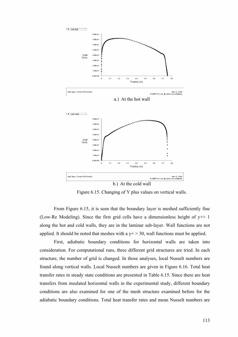
113

a.) At the hot wall

b.) At the cold wall

Figure 6.15. Changing of Y plus values on vertical walls.

From Figure 6.15, it is seen that the boundary layer is meshed sufficiently fine

(Low-Re Modeling). Since the first grid cells have a dimensionless height of y+≈ 1

along the hot and cold walls, they are in the laminar sub-layer. Wall functions are not

applied. It should be noted that meshes with a y+ > 30, wall functions must be applied.

First, adiabatic boundary conditions for horizontal walls are taken into

consideration. For computational runs, three different grid structures are tried. In each

structure, the number of grid is changed. In those analyses, local Nusselt numbers are

found along vertical walls. Local Nusselt numbers are given in Figure 6.16. Total heat

transfer rates in steady state conditions are presented in Table 6.15. Since there are heat

transfers from insulated horizontal walls in the experimental study, different boundary

conditions are also examined for one of the mesh structure examined before for the

adiabatic boundary conditions. Total heat transfer rates and mean Nusselt numbers are

114

given for different boundary conditions in Table 6.16 and Table 6.17, respectively. In

Figures 6.16, 6.17, 6.18 and 6.19, change of local Nusselt numbers are given for four

different boundary conditions. It is seen that nearly similar local Nusselt numbers are

obtained for vertical walls. However mean Nusselt numbers horizontal walls for BC 4

are closer to values obtained by experimental study. The source for the difference is

researched. It is thought that the difference can stem from the turbulence model used.

Since the heat flow rates and mean Nusselt numbers obtained by BC 4 are much closer

to values obtained by an experimental study. Therefore total heat transfer rates and

mean Nusselt numbers are compared in different turbulence models for BC4 and

number of elements of 40 000. The results are given in Table 6.18 and 6.19.

Table 6.15. Mean Nusselt numbers for three different grid sizes in adiabatic boundary conditioned horizontal walls.

Number of cells Wall Experimental

22 500 40 000 62 500

Hot 62.9 61.61 61.67 61.672

Cold 62.6 61.61 61.69 61.691

Figure 6.16. Local Nusselt numbers on the vertical walls for the adiabatic boundary

condition (Number of cell is 22 500).

115

Table 6.16. Total heat transfer rates (W) from the walls and reference temperatures for different boundary conditions (Number of cells is 40 000).

Boundary Conditions .

Experimental

BC 1 BC 2 BC 3 BC 4

Bottom wall 21.67 0 21.67 7.45 17.71

Cold wall 97.77 95.9 83.81 92.22 85.82

Hot wall 98.12 95.9 84.67 91.97 85.28

Top wall 22.53 0 -22.53 -7.2 -17.17

Table 6.17. Mean Nusselt numbers for three different grid sizes in different boundary conditions (Number of cells is 40 000).

Experimental BC 2 BC 3 BC 4

Cold wall 62.6 53.95 61.54 55.2

Hot wall 62.9 54.49 61.54 54.83

Bottom wall 13.9 13.95 0.015 11.45

Top wall 14.4 14.5 0.015 11.09

Figure 6.17. Nusselt numbers for the boundary condition 2.

116

Figure 6.18. Nusselt numbers for the boundary condition 3.

Figure 6.19. Nusselt numbers on the vertical walls (k-epsilon turbulence model and

viscous effects are neglected).

117

Table 6.18. Total heat transfer rates (W) from the walls for investigated turbulence models (for boundary condition IV and number of cells is equal to 40 000).

Wall k-ε Standard k-w SST k-w

Bottom 17.71 16.48 16.06

Cold 85.82 84.37 84.82

Hot 85.28 83.71 84.22

Top 17.17 15.81 15.46

Table 6.19. Mean Nusselt numbers for different turbulence models (for boundary condition 4).

Wall k-ε Standard k-w SST k-w

Bottom 11.45 10.66 10.39

Cold 55.2 54.27 54.55

Hot 54.83 53.82 54.15

Top 11.09 10.21 9.99

As a result of applying different two equation turbulence models, close values

are found for mean and local Nusselt number as seen in Table 6.19. The difference can

be sourced from 3D turbulent flow in experimental set up. They used cross sectional

area to find 2D flow as explained in Chapter 4. It is evaluated that using correct

boundary conditions in computational solutions gives realistic results.

118

CHAPTER 7

BOUNDARY CONDITIONS AND

COMPUTATIONAL DETAILS

The computational study is accomplished for the tested radiators by using

ICEPAK software. Before some preliminary analyses are realized to solve three

dimensional natural convection problem.

7.1. Pre-Analysis

Since, only one side which is located at the behind of the radiator is insulated in

the examined problem, two dimensional cavity whose one of the vertical sides is hot

and remaining three sides are colder is solved at the beginning. Then the hot wall is

replaced by partially heated wall. Finally, the hot wall is replaced by insulated wall and

there is a rectangular domain whose surface temperature is being constant. All two

dimensional cases are model in GAMBIT and solved by FLUENT. When two

dimensional results are found logical, three dimensional case with an internal object

having constant surface temperature is solved.

7.1.1. Natural Convection in Cavity with Three Cold and One Hot Sides

Three cases are examined. The boundary conditions of first case are given

below. Temperatures of cold sides are 293 K (20oC). The hot side temperature is 343 K

(70oC).

On vertical walls;

cy TLxy ===<<= T 0;VV ,0 ,0 x (L=4 000 mm),

cy TLxHy ===<<= T 0;VV ,0 , x (H=3 000 mm) At horizontal walls;

119

Cx TT 0;VV ,0 ,0 ===≤≤= yHyx

hx TT 0;VV ,0 , ===≤≤= yLyLx

Since one of the termination criteria is total heat transfer from the cavity, the

heat transfer rates at each wall are followed during analysis. At steady state, the net heat

transfer rates from the cavity is zero. The heat transfer rates at steady state are given in

Table 7.1. The heat transferred to outside of the cavity is denoted by minus sign.

Table 7.1. Total heat transfer rates from the walls and reference temperatures in different number of elements for two dimensional cavity which has three cold and one hot sides (W).

Number of cells 30 000 58 800 82 400

Bottom cold wall -21.78 -21.75 -21.765

Left Cold wall -183.32 -184.25 -184.28

Hot wall 545.3 547.59 547.56

Top cold wall -340.18 -341.57 -341.58

Reference Temp. (K) 306.28 306.29 306.293

Contours of stream function is given in Figure 7.1 a. Contours of y and x

velocities are plotted in Figure 7.1 b.) and 7.1 c.), respectively.

120

a.)

b.)

c.)

Figure 7.1. Contours obtained for the cavity whose three side is cold and the other side is hot.

121

7.1.2. Cavity with Three Cold and One Partially Heated Sides

The second case in which air is heated from some part of the one vertical wall

and cooled from three sides is solved next. The boundary conditions of the second case

are explained below. Temperatures of cold sides are 293 K (20 oC). The hot side

temperature is 343 K (70 oC).

Horizontal walls;

T 0;vu ,0 ,0 c===<<= TLxy

cT 0;vu ,0 , ===<<= TLxHy Vertical walls;

CTT 0;vu ,0 ,0 ===≤≤= Hyx

0dxdT 0;vu ,0 100 , ===≤≤= HyLx

L=4 000 mm, H=3 000 mm

In Table 7.2, total heat transfer rates from walls are summarized for the steady

state condition. Stream function, temperature and Y velocity contours are plotted in

Figure 7.2.

Table 7.2. Total heat transfer rates (W) from the walls and reference temperatures for two dimensional domain which has three cold and one partially heated side.

Number of cells 30 000 58 800 82 400

Bottom cold wall -22.4 -23.06 -23.08

Left cold wall -88.23 -86.56 -86.54

Hot wall 254.74 255.47 255.4

Top cold wall -144.07 -145.68 -145.63

Insulated Wall 0 0 0

h, 0 1 000, u v 0; T Tx L y= ≤ ≤ = = =

122

a.)

b.)

c.)

Figure 7.2. Contours obtained for the cavity which has three cold and one partially heated side.

123

7.1.3. Natural Convection in the Cavity with Internal Heated Body

The schematic view of the investigated case is given in Figure 7.3. In this case,

the internal body has constant surface temperature (343 K, 70 oC). The temperatures of

cold sides are 293 K (20 oC). The rectangular shaped body does not include any mesh

since only the flow around the body is solved. During the analysis the reference

temperature has been followed as heat transfer rates from walls. In Table 7.3, those

values are presented. Contours for the considered case are plotted in Figure 7.4.

Figure 7.3. The schematic view of cavity with internal heated body.

Table 7.3. Total heat transfer rates from the walls (W) and reference temperatures for cavity with internal heated body.

Number of cells 19 420 39 600 59 832 72 840 89 360

Bottom cold wall -47.76 -51.11 -50.60 -55.41 -53.4

Left cold wall -153.22 -152.94 -152.26 -155.45 -155.31

Right wall (insulated) 0 0 0 0 0

Top cold wall -247.49 -249.75 -253.78 -256.44 -257.68

Hot Wall 449.11 453.71 465.01 467.57 466.62

Reference Temp. (K) 305.22 305.61 305.33 305.66 305.69

gLeft cold wall

Top cold wall

Bottom cold wall L

H

x,u

y,v

L=4000 mm, H=3000 mm

Hot walls

Insulated wall

124

a.)

b.)

c.)

Figure 7.4. Contours for cavity with internal heated body.

It is evaluated that reasonable results are obtained for the flow in cavity with

high Rayleigh numbers. Air flows from bottom to top near the hot vertical wall while

125

from top to bottom horizontal walls near the cold vertical wall. Circular stream function

contours are deformed when they compared with the stream function contours obtained

for square cavities.

7.1.4. Natural Convection in a Three Dimensional Enclosure with an Internal Heated Body

A three dimensional object whose surface temperatures are being kept constant

is investigated in this section. Dimensions of this three dimensional geometry is similar

with the dimensions of single panel radiator. This problem is solved by using ICEPAK.

The surface temperature is assumed to be equal to the average of inlet and outlet water

temperature measured in the single panel test which is 75.22oC. The temperatures of test

room walls are 18.5oC except for the wall behind the radiator. Thermal impedance of

this wall is 2.5 oCm2W-1. Since there is an oscillation in residuals of some steady state

solution of natural convection problems, time marching approach is used to obtain

steady state solution in this problem. Analysis was realized for two different grid

structures. In the second grid structure, the number of elements is decreased by 35%.

Discrete ordinate radiation model was used with its default settings in the ICEPAK

interface. A two equation turbulence model was used for simulation of turbulent air

flow around the radiator. Body forced weighted pressure discretization is selected while

first order scheme is applied in equations of momentum, energy and turbulence.

Because of the natural convection heat transfer, under relaxation factors for pressure,

momentum and energy are 0.3 and 0.3, 0.96, respectively. Default values are used for

the other under relaxation factors (1.0 for viscosity, body forces and 0.5 for turbulent

kinetic energy and turbulent dissipation rate). Bousinessq approach (Chapter 2) and

double precision is used in the analysis.

Extra two termination criteria are applied during the analysis: reference air

temperature and air velocity near the top of the radiator. The stability in these criteria is

taken into consideration. When stability is seen in these factors, the analysis is stopped.

126

Table 7.4. Number of elements in two different grid structures generated for 3D enclosure with internal body.

GRID I GRID II GRID III GRID IV

Number of Elements 29 120 44 800 156 230 951 048

Number of Nodes 32 076 48 708 158 040 989 330

a.)

b.) Top view of grid

Figure 7.5. The sectional view of grid created for 3D domain (Grid II).

Figure 7.6. The temperature contour (oC) at vertical plane (II-II) whose normal is in the

z direction (Grid II).

II II

III III

Heater

127

Symetricity in temperature contours in the middle section of virtual test room

occurs as expected. Nearly horizontal lines are found at the bottom part of the virtual

test room.

Figure 7.7. The velocity contour (oC) at vertical plane (II-II) whose normal is in the z

direction (Grid II).

Velocity contours in the vertical plane where the temperature of reference point

is measured will be symmetrical when surface temperature is constant or uniform.

Figure 7.8. The temperature contour (oC) at vertical plane (III-III) whose normal is in

the x direction (Grid II)

128

Hot region occurs near the middle part of the top horizontal surface of the virtual

test room. Symetricity in temperature contours is seen in all sections of virtual test room

as occurs near the heated object.

Figure 7.9. The temperature contour at vertical plane (I-I) whose normal is in the x direction (Grid II and x=2.398)

The hot region occurs around the heater, the air temperature throughout the

virtual test room is approximately 20oC in the middle plane whose normal is in x

direction.

Figure 7.10. Y velocity contours at vertical plane (I-I) whose normal is in x direction (Grid II).

129

Hot air goes up around the heater while cold air flows to the bottom surface at

the opposite side of the heater.

a.) At vertical plane (I-I) whose normal is in the x direction (Grid II)

b.) Around the heater

Figure 7.11. Velocity vectors (Grid II).

Table 7.5. Total heat transfer rates in different grid structures.

GRID Turbulence Model Heat Transfer Rate (W)

k-ε 376.225 I

Realizable k-ε 376.30

II k-ε 377.823

III k-ε 377.821

IV k-ε 377.820

130

7.2. CFD Analysis of Tested Radiators

In this section the details of computational study for tested radiators are

presented.

7.2.1. ICEPAK Models for Tested Radiators

CFD models for the tested radiators (Radiator I, II and III) are shown in Figure

7.12. They are prepared in ICEPAK software. Because of the difficulties in radiator

geometries rounds are ignored. Dimensions are same except at the cross sectional area

of vertical water channels. Since cubical elements can be meshed properly in ICEPAK,

the water volume in gaps is simplified. A detailed view of CFD model of a single panel

is given in Figure 7.13.

In CFD models, air and water volumes are created from solid rectangular prisms

at the beginning. Their material properties are changed from solid to fluid, later. Water

is assigned as a default fluid while air is defined as a secondary fluid. Because priority

is important in ICEPAK modeling. When two intersecting blocks are drawn, the late

generated object whose priority is high is meshed before. Also boundary conditions and

material properties of the late generated object is used in the intersection. As a result of

pressing two steel sheets, a solid region is created as seen in Figure 7.14-b. Those parts

are modeled by solid blocks. All steel shells which located around water channels are

modeled by conducting thin plate whose thickness is zero. However thickness and

conductivity are taken into consideration in the calculations. Only steel sheets shown in

Figure 7.14-a are made from the solid blocks. The effective thickness and material of

the thin plates are determined.

131

a.) Radiator I

c.) Radiator II d.) Radiator III

Figure 7.12. ICEPAK models of tested radiators.

Figure 7.13. Details of CFD model of single panel.

132

Figure 7.14. Comparison of real and CFD models.

7.2.2. Mesh Details

Four different grid structures in which number of elements is changed are tried

in CFD analysis of Radiator I (case 1) as seen in Table 7.6. Since the results of last two

grid structures (C-I and D-I) are similar for Case 1, other cases (Case 2 and Case 3) are

solved with only C-I and D-I for Radiator I.

Table 7.6. Mesh details for Radiator I.

A-I B-I C-I D-I

Number of Elements 831 784 1 111 492 1 472 646 3 159 224

Number of Nodes 879 723 1 173 042 1 548 356 3 266 230

Uniform grid structure is preferred at the region represents the test room air in

CFD model of radiator I as shown in Figure 7. 14. The grid density had been increased

around the walls of the virtual test room and tested radiators as seen in Figure 7.15.

133

Figure 7.15. A cross sectional view of grid created in the virtual test room which includes radiator I.

Figure 7.16. The grid density around radiator I.

Similar strategy was used in the preparation of CFD models of radiator II and

III. The cross sectional views of grids are presented in Figure 7.17 and 7.19 for other

CFD models of investigated radiators. Also for those models, grid densities were

increased around the panel and extended surfaces as shown in Figure 7.18 and 7.20.

134

Figure 7.17. A cross sectional view of grid created for the test room includes radiator II.

Figure 7.18. The grid density around radiator II.

Table 7.7. Mesh details for three cases of Radiator II.

A-II B-II

Number of Elements 1 727 060 2 147 514

Number of Nodes 1 816 385 2 248 135

135

Figure 7.19. A cross sectional view of grid created for the test room includes radiator III.

Figure 7.20. The grid density around radiator III.

Table 7.8. Mesh details for three cases and Radiator III.

A-III B-III

Number of Elements 2 670 998 3 198 404

Number of Nodes 2 760 778 3 303 414

7.2.3. Boundary Conditions

Since three test conditions are defined in EN 442 part 2 standard for tested

radiators, the computational study is performed with applying different boundary

136

conditions. In each case, the inlet water velocity is defined with its temperature. Inlet

velocity is calculated by using Equation (7.1).

win

w

mVAρ

=⋅

(7.1)

Where ρw is density of water circulated through the hollow section of radiator

and A is the cross-sectional area of inlet section. For the considered problem,

rectangular water channels whose hydraulic diameters are equal to circular connection

pipes are used in the computational study. These channels are assumed insulated as in

real tests. Their cross sectional areas are 169 mm2. Water density is assumed 1 000

kg/m3 for the calculation of inlet velocity. The temperature values are taken from real

tests. Average values are used to determine inlet boundary conditions. Velocity and

temperature of inlet water are defined as summarized in Table 7.9, in the analysis.

Table 7.9. Boundary conditions at radiator inlet.

Radiator Case Tin (oC) Vin (m/s)

1 75.22 0.1028

2 86.56 0.1031 I

3 52.48 0.1029

1 74.81 0.1354

2 86.15 0.1348 II

3 52.70 0.1353

1 75.41 0.2539

2 89.97 0.2545 III

3 53.21 0.2548

Since several steady runs are performed for all models and each case. The steady

state results are attained in those computational performances. At the beginning runs

wall temperatures are kept at 20oC. When reference temperature is constant, the wall

temperatures are changed and new iteration is initiated.

In the final runs, constant temperature boundary conditions with no slip

conditions are specified at all horizontal and vertical walls of virtual test room as given

in Table 7.10.

137

Table 7.10. Boundary conditions for the walls of virtual tests room (except wall behind tested radiators).

Radiator Case Temp(oC)

1 19.5

2 19 I

3 20

1 19

2 18.5 II

3 19.5

1 18.5

2 18 III

3 19

7.2.4. Assumptions and Solver Settings

Certain assumptions as given below are made in order to facilitate the analyses.

• Air flow is assumed incompressible turbulent.

• Ambient air is assumed 20oC.

• Boussinesq approximation is used.

• The gravity is set to 9.806 ms-2.

• Steady state analysis are performed.

• Very small velocity on y direction (0.001 m/s) is put as an initial value at the

beginning of runs.

• Because the mesh is not coarse and existence of small cells, double precision is

preferred.

• SIMPLE algorithm is used to model the interaction between pressure and

velocity.

• In order to speed up the solution times, first-order upwind scheme is applied for

continuity, momentum and energy equations in first runs. Last runs when the

first order solution approaches convergence, the second order discretisation

scheme is enabled.

• k-ε turbulence model is used.

138

7.2.5. Convergence Criteria

Computational run for one case of a radiator was completed in 7 days by using a

computer having 12 GB Ram and 3GHz Processor. Trial periods are not included to

computational run times. One of the reasons for long run times is using only one

processor because of the restriction when shell conduction is used in the analysis.

In this study, change in temperature of reference point and velocity near the

virtually tested radiator are controlled by assignment of several points during analyses.

It is observed that oscillations in temperature can be seen when coarse mesh is used.

Several runs are performed for one radiator type to find steady state conditions in the

virtual test room. It is evaluated that when the temperature of reference point and

residuals are being controlled only, specious results can be obtained. Velocities cannot

be reached steady state values although controlled temperature is being constant. In this

study, the CFD runs were stopped as velocities near the tested radiator becomes. To

shortened run times, several runs were performed for each radiator and case. One run

was stopped when the reference air temperature became constant. The next run was

initiated with last solution data and stopped when velocities were constant. Changing of

scaled residuals in continuity, u velocity, v velocity, w velocity, energy, k, ε and

discrete ordinate intensity as explained in Chapter 2 are also followed.

Changing of parameters which are followed are given in Figures 7.21, 7.22 and

7.23 for Radiator II and Case 1 as an example. In all runs, same controlling mechanism

is used to understand whether the flow is reached the steady state condition.

Convergence criteria for residuals of flow, energy, turbulent kinetic energy and

turbulent dissipation rate are 0.0001, 10-7, 10-7, and 10-7, respectively.

139

1.E-08

1.E-07

1.E-06

1.E-05

1.E-04

1.E-03

1.E-02

1.E-01

1.E+00

0 500 1000 1500 2000

Number of Iterations

Solu

tion

Res

idua

ls

continuity u v w energy k ε do-intensity Figure 7.21. Residuals in the final CFD run for radiator II (Case 1).

292.60

292.80

293.00

293.20

293.40

293.60

293.80

294.00

0 500 1000 1500 2000

Number of Iteration

Ref

eren

ce P

oint

Tem

pera

ture

(K)

Figure 7.22. Reference point temperature in the final CFD run for radiator II (Case 1).

0.3

0.4

0.5

0.6

0 500 1000 1500 2000Number of Iteration

Vel

ocity

(m/s)

Air velocity at bottom part of radiator II (case 1)Air velocity at middle part of radiator II (Case 1)Air velocity at top of the radiator II (Case 1)

Figure 7.23. Air velocities in the final CFD run for radiator II (Case 1).

140

7.2.6. Comparison of Results

Computational and experimental results are compared by using Equation (7.2).

By this way, the closeness of computational and experimental results is determined.

exp

exp

100% compQ Q

DifferenceQ− ⋅

= (7.2)

141

CHAPTER 8

RESULTS AND DISCUSSION

Heat outputs of tested three radiators were determined by using a commercial

finite volume solver in this study. Temperature distributions at front dry surfaces and

horizontal cross sections of investigated radiators were examined in the post processing

part. Also velocity and temperature distributions in selected sections of the virtual test

room were investigated apart from the experimental study.

Finally, experimental and computational heat outputs of tested radiators were

compared to find correctness of numerical results. Since three operating conditions were

taken into consideration in the experimental part, computational study was also

accomplished for considered conditions. Results are presented for all examined cases.

8.1. CFD Results for Radiator I

CFD model of radiator I is the simplest model examined in this study.

Temperature distributions on vertical mid plane of CFD model of radiator-I are shown

in Figure 8.1. It is detected that the hot water passes from the channels near to support

line mostly. The bottom opposite side to the inlet section is the coolest part of radiator.

Unfortunately, the temperature measurements from radiator surfaces are not specified in

EN 442 standard. If temperature from the dry surfaces of the radiator is measured in the

experimental study, it will be non equal in different points throughout the surface. The

thermal camera views presented in Chapter 5 show non equal temperatures at the front

surface. From the CFD results the non-uniform temperature distribution occurs at the

front surface are also seen. Figure 8.2 in which temperature distribution at three

different horizontal cross sections are drawn also illustrates that coolest water is

collected at the bottom end of the radiator. Temperature distributions at two vertical mid

planes are given in Figure 8.3 and Figure 8.4. Symmetric temperature contour lines are

noticed in Figure 8.3. Effect of heating is shown in Figure 8.4. Temperature contours at

the horizontal mid plane of virtual test room is given in Figure 8.5. The propagation of

142

temperature fields are demonstrated clearly in this figure. The symmetric lines are also

observed above the radiator.

a.)Case 1

b.)Case 2

c.)Case 3

Figure 8.1. Temperature distribution on vertical mid plane of radiator I (z=0.4559 m).

143

a.)Case 1

b.)Case 2

c.)Case 3

Figure 8.2. Temperature distributions at three different horizontal cross sections of radiator I.

144

a.) Case 1

b.) Case 2

c.) Case 3

Figure 8.3. Temperature contours on the vertical mid plane of virtual test room whose normal is in z direction (z=2.405 m).

145

a.) Case 1

b.) Case 2

c.) Case 3

Figure 8.4. Temperature contours on the vertical mid plane of virtual test room whose normal is in x direction (x=2.398 m).

146

a.) Case 1

b.) Case 2

c.) Case 3

Figure 8.5. Temperature contours on the horizontal mid plane of virtual test room whose normal is in y direction (y=1.867 m).

Hot region occurs the near to radiator in the virtual test room. In Figure 8.6,

velocity contours are drawn with regard to velocity magnitude.

147

a.) Case 1

b.) Case 2

c.) Case 3

Figure 8.6. Velocity contours on the vertical mid plane of virtual test room whose normal is in z direction (z=2.405 m).

148

From Figure 8.6, it is seen that the velocity in the midde section is quite low.

Velocity increases up to horizontal surfaces of virtual test room. Although there is a

symetricty in velocity contours, it becomes to change.

Computational heat outputs in three different operating conditions are presented

in Table 8.1. Computational (obtained from C-I grid structure) and experimental heat

outputs are given together in Table 8.2.

Table 8.1. Computational heat outputs of radiator I in different grid structures (W).

Table 8.2. Compared heat outputs for radiator I (W).

Case I Case II Case III

Computational (QD-I) 739.8 953.8 393 Experimental (Qexp) 736.5 902.1 346.0

8.2. CFD Results for Radiator II

CFD model of radiator II includes fins attached to panel as described in Chapter

7. Temperature distributions on vertical mid plane of panel of radiator II are shown in

Figure 8.7. Effect of extended surfaces is seen in Figure 8.7. The coolest region is closer

to bottom part of the radiator. The temperature distribution on horizontal cross section is

given in Figure 8.8. When those illustrations are taken into consideration same problem

seen for radiator I is observed. The surface temperatures are not uniform for radiator II.

Temperature distributions at several sections of the virtual test room are given in

Figures 8.9 and 8.10. Velocity contours at the middle plane of the virtual test room are

presented in Figure 8.11. The motion of air is shown in Figure 8.12 for radiator II. The

beginning section is selected as the rear side of the radiator. Velocities are higher above

the radiator. Particles move to radiator from all side of the test room

Case QA-I QB-I QC-I QD-I 1 962.33 821.15 743.27 739.8 2 - - 964.87 953.8 3 - - 391.15 393

149

a.)Case 1

b.)Case 2

c.)Case 3

Figure 8.7. Temperature distribution on vertical mid plane of panel used in radiator II.

150

a.)Case 1

b.)Case 2

c.)Case 3

Figure 8.8. Temperature distribution on a horizontal cross section of radiator II.

151

a.)Case 1

b.)Case 2

c.)Case 3

Figure 8.9. Temperature contours on the vertical mid plane whose normal is in z direction (z=2.405 m).

152

a.) Case 1

b.) Case 2

c.) Case 3

Figure 8.10. Temperature contours on the vertical mid plane whose normal is in x direction (x=2.398 m).

153

a.) Case 1

b.) Case 2

c.) Case 3

Figure 8.11. Velocity contours on the vertical mid plane whose normal is in z direction (z=2.405 m).

154

Figure 8.12. Path lines for the air motion in virtual test of radiator II.

Heat outputs in three different cases for radiator II are presented in Table 8.3.

The comparisons between computational heat outputs obtained from the second grid

structure with experimental heat output are given in Table 8.4.

Table 8.3. Computational heat outputs (W) of radiator II in two different grid structures.

Table 8.4. Compared heat outputs for radiator II.

Case 1 Case 2 Case 3

Computational (QA-ıı) 1 001.56 1 302.38 544.07 Experimental (Qexp) 968.42 1 210.25 489.87

Case QA-II QB-II I 1 004.18 1 001.56

II 1 307.93 1 302.38

III 546.80 544.07

155

8.3. CFD Results for Radiator III

Path lines are given in Figure 8.13 for radiator III. As it is seen from the figure,

the flow of air becomes more complicated in the virtual test of radiator III. Temperature

distributions on vertical mid plane of panel used in radiator III and in Case 1, Case 2

and Case 3 are shown in Figure 8.14, Figure 8.15 and Figure 8.16, respectively. Since

there are two panels in radiator III, the temperature distributions on front and back

panels are given separately. Velocity and temperature contours obtained for radiator III

are given in Figure 8.17 and 8.18, respectively. As it is seen from Figure 8.17, the

symmetricity is broken down in excess temperature of 60oC. The computational heat

outputs in three different cases are presented in Table 8.5. Experimental and

computational heat outputs are given in Table 8.6. Comparison of results is given in

Table 8.7.

Figure 8.13. Pathlines for the air motion in virtual test of radiator III.

156

a.)Vertical mid plane on back panel.

b.)Vertical mid plane on front panel.

c.)Horizontal cross section.

Figure 8.14. Temperature distribution on radiator III in case 1.

157

a.)Vertical mid plane on back panel

b.)Vertical mid plane on front panel

c.)Horizontal cross section


158

a.)Vertical mid plane on back panel.

b.)Vertical mid plane on front panel.

c.)Horizontal cross section.


159

a.)Case 1

b.)Case 2

c.)Case 3

Figure 8.17. Velocity contours on the vertical mid plane whose normal is in z direction (z=2.405 m).

160

a.) Case 1

b.) Case 2

c.) Case 3

Figure 8.18. Temperature contours on the vertical mid plane whose normal is in z direction (z=2.405 m).

161

Table 8.5. Computational heat outputs of radiator III in two different grid structures (W).

Table 8.6. Experimental heat outputs of radiator III (W).

Case 1 Case 2 Case 3

Computational 1 983.46 2 395.15 997.34

Experimental 1 898.58 2 213.56 883.25

In Table 8.8, experimental and computational heat outputs are compared by using

Equation (7.2) for all tested radiators.

Table 8.7. Comparison of heat outputs of tested radiators.

Radiator Case 1 Case 2 Case 3

I 0.4 5.7 13.6

II 3.4 7.6 11.1

III 4.5 8.2 12.9

From the steady state analyses performed for the tested radiators, relatively

closer results are obtained for the first case. It should be noted that the standard heat

output of radiators are determined according to Case 1. The difference between

experimental and computational heat output in percentage fluctuate between 0.4 and

13.6 for the simplest model (radiator I), 3.4 and 11.1 for the second CFD model radiator

(radiator II), 4.5 and 12.9 for most complicated model investigated in this study. Quite

good results are obtained for the excess temperature of 50oC and 60oC. For the lowest

excess temperature, results are also in acceptable range. It is considered that difference

can be sourced from turbulence model, radiation model, using Boussinessq

approximation and errors seen in CFD process as mentioned in Chapter 2.

Case QA-II QB-II 1 1 990.05 1 983.46

2 2 399.37 2 395.15

3 1 003.11 997.34

162

CHAPTER 9

CONCLUSION

The aim of this study is investigating whether numerical methods are applicable

in the determination of heat output of radiators. One of the important advantages of

using CFD software in this problem is that it enables to control flow properties like

temperature and velocity at more than one point in the virtual test room. On the other

hand, measuring of temperature and velocity is not easy and measuring devices require

calibration. CFD solutions need experimental validation.

At the beginning, experimental heat output of radiators was determined in the

test room designed with regard to EN 442 part 2 standard. Three operating conditions

are taken into consideration in the test period: excess temperature of 50oC, 60oC and

30oC. The measurements specified in the standard are notoriously difficult because of

the number of limitations controlled simultaneously during tests. One test for a radiator

was completed approximately in six hours in this study. All tests were completed in four

days. Test duration can be longer when inexperienced test operators perform tests.

First computational study was investigation of correctness of solution obtained

by selected commercial software for natural convection in cavity. Since numerical

results obtained by using FLUENT software well match with results given in Literature,

finite volume solver of FLUENT was accepted to use in the study. Since ICEPAK uses

same solver with FLUENT, it was preferred for the determination of computational heat

output of radiators.

It is evaluated that the quality of the numerical predictions depends on the

accurate modeling of problems and fine grid structure. One of the important advantages

of using ICEPAK is that the generation of CFD models and grids are relatively simpler

in ICEPAK. Although automatic mesh generation is an advantage in ICEPAK, the

skewness of elements in grid structure must be checked. Manual grid generation is

always advised. In addition, using different under relaxation factors automatically in

ICEPAK facilitates convergence. Properties of the problem given below complicate the

solution with numerical methods:

163

– two fluid flows,

– large solution domain,

– difficulty of mesh generation for thin walls used in the radiator geometry,

– shell conduction,

– turbulent type of natural convection

– radiation

– changing wall temperature boundary condition for virtual test room

– not applying symmetric boundary conditions

It should be mentioned that three dimensional CFD models are computationally

expensive than two dimensional models. As an example, the CFD model of a single

panel radiator (radiator I) was prepared in two week. The solving time was nearly one

week.

CFD model of single panel radiator with single extended surface (radiator II)

and double panel with double extended surface (radiator III) prepared faster since CFD

model of single panel radiator has existed.

Convergence of solutions in natural convection is generally difficult with regard

to forced convection applications. In the solution of natural convection problems,

oscillations and difficulties in convergence can be faced. In such situations, different

strategies can be applied. One approach is using time marching approximation. In this

study, the steady state solver is used. The velocity of air at some points near the tested

radiator is controlled in addition to change in residuals and temperature of reference air

during the analysis. When the constant reference air temperature is obtained and

convergence criteria for residuals are realized, it is decided that the steady state solution

is obtained. However computational runs are restarted several times with previous data

file and terminate up to getting constant velocities. Therefore stopping criteria are

reference air temperature, residuals and velocity near tested radiators.

Controlling reference air temperature with changing wall temperatures makes

CFD analysis quite difficult. Since such control mechanism is not used in commercial

CFD software. Wall temperatures are settled manually and this brings about loss of time

and labor.

Unknown standard mass flow rate is another difficulty faced in virtual test room.

Without having mass flow rate knowledge, the CFD analysis can also be made. Number

of iterations to find the proper mass flow rate can increase the solution time.

164

From the steady state analyses performed for the tested radiators, relatively

closer results are obtained for the simplest model (radiator I). However closeness of

experimental and computational heat outputs is decreased with complexity of CFD

model. In spite of using non real geometries for radiators, the deviation between

experimental and computational results is maximum 13.6%. The difference between

experimental and computational heat output in percentage fluctuate between 0.4 and

13.6 for the simplest model (radiator I), 3.4 and 11.1 for the second CFD model

(radiator II), 4.5 and 12.9 for most complicated model investigated in this study. Quite

good results are obtained for the excess temperature of 50oC and 60oC. For the lowest

excess temperature, results are also in acceptable range.

The results indicate that determination of heat output by numerical methods is

possible and reliable but not adequate. Especially the closeness of computational and

experimental standard heat output of a radiator which is determined at the excess

temperature of 50oC (Case 1) is attractive. However increment in difference between

experimental and numerical heat output for Case 3 is found unsatisfying. The results

also show that using simpler geometries in which rounds are ignored did not affect the

heat output of radiators in CFD analysis.

Non uniform temperature distribution on the front surface of tested radiators was

observed in the experimental study. Similar temperature distributions were also seen at

the end of the computational study as given in Chapter 8. It is considered that the

uniform cross sections of vertical channels in the radiator should be reassessed in the

design of new radiators.

When temperature and velocity contours are examined throughout the test room.

It is seen that velocity and temperature contours in the vertical plane where the

temperature of reference point is measured will be symmetrical when the heater surface

has constant or uniform temperature.

Almost symmetric velocity and temperature contours are also seen when single

panel radiator is used in the virtual test room. Since non uniform temperature

distribution occurs in the front and back surfaces of radiator, the symmetricity in

velocity contours is broken down by using more complicated radiators. Especially with

increasing excess temperature difference, the structure of velocity contours is extremely

changed.

165

According to findings in this study, it is evaluated that the numerical solution of

this problem can be useful in design of new types of heaters in future works. However,

long solving time is accepted as a serious problem for the real life.

It is thought that the difficulties sourced from the preparation of CFD model and

mesh generation will not be seen in future, parallel to development in CFD software and

computers specifications. Instead of measuring only reference air temperature,

measurements of velocity and temperature from more points in the real test room are

planned as a future study to compare the basic characteristics of flow in the enclosure.

Determination of surface emissivity of test room will be useful in the future analysis.

Controlling of temperature boundary conditions of test room panels with regard to

change in reference point temperature can decrease the solving time in future analysis.

166

REFERENCES

Ampofo F, Karayiannis TG. 2003. Experimental benchmark data for turbulent natural

convection in an air filled square cavity. International Journal of Heat and Mass Transfer 46: 3551-3572.

André B. Computational Fluid Dynamics Course Notes. Dartmouth College; [cited 2010 June 10]. Available from: http://www.bakker.org/dartmouth06/engs150.

ANSYS FLUENT 12.0 User and Theory Guides, April 2009.

Ashgriz N, Mostaghimi J. An Introduction to Computational Fluid Dynamics, Chapter 20, Fluid Flow Handbook, Department of Mechanical & Industrial Eng. University of Toronto.

ASHRAE Systems and Equipment Handbook (SI). Hydronic Heat-Distributing Units and Radiators. 2000.

Aydin O, Unal A, Ayhan T. 1999. Natural convection in rectangular enclosures heated from one side and cooled from the ceiling. International Journal of Heat and Mass Transfer 42: 2345-2355.

Awbi HB. 1989. Application of Computational Fluid Dynamics in Room Ventilation. Building and Environment, 24(1),73-84.

Balaji C , Venkateshan SP. 1993. Interaction of surface radiation with free convection in a square cavity. Int. J. Heat and Fluid Flow 14 (3): 260-267.

Beck SMB, Grinsted SC, Blakey SG, Worden K. 2004. A novel design for panel radiators. Applied Thermal Engineering 24: 1291–1300.

Bilir L. 2009. Numerical Optimization of a Finned Tube Gas to Liquid Heat Exchanger. PhD diss., Izmir Institute of Technology.

Callister W. 1985. Materials Science and Engineering An Introduction. John Wiley & Sons.

Cengel Y. 2006. Heat and Mass Transfer A Practical Approach, McGraw Hill, CRC PRESS.

Chang YP, Tsai R. 1997. Natural Convection in a Square Enclosure with a Cold

Surface. Int. Comm. Heat and Mass Transfer. 24 (7): 1019-1027.

167

Dağsöz, AK. 1998. Sıcak Sulu Kalorifer Tesisatı, Demirdöküm Teknik Yayınları No:6.

Davis V. 1968. Laminar Natural Convection in an Enclosed Rectangular Cavity. Int.J. Heat Mass Transfer 11:1675-1693.

European Standard EN 442-2. 1997. Radiators and convectors- Part 2: Test methods and rating.

Hyun J, Lee JW. 1989. Numerical solutions for transient natural convection in a square cavity with different sidewall temperatures. Int. J. Heat and Fluid Flow. 10 (2).

Ganzarolli M, Milanez LF. 1995. Natural Convection in rectangular enclosures heated from below and symmetrically cooled from the sides. Int. J Heat Mass Transfer. 38 (6): 1063-1073.

Gritzki R, Perschk A., Rösler M., Richter W. 2007. Modelling of Heating Systems and Radiator in Combined Simulations. Proceedinngs of Clima 2007 WellBeing Indoors.

Kakac S, Shah RK, Aung W. 1997. Handbook of Single –Phase Convective Heat Transfer. John Wiley&Sons. Inc.

Laser Doppler Anemometry [Internet]. Tampere University of Technology; [cited 2010 June 10]. Available from: http://www.tut.fi/units/me/ener/laitteistot/EFD/LDA.html.

Markatos NC, Pericleous KA. 1984. Laminar and turbulent natural convection in an enclosed cavity. International Journal of Heat and Mass Transfer. 27(5): 755-772.

Menter F. EUROPEAN COMMISSION. 2002. CFD Best Practice Guidelines for CFD Code Validation for Reactor Safety Applications, 5th EURATOM FRAMEWORK PROGRAMME 1998-2002.

Modest, M.F. 2003. Radiative Heat Transfer, Second Edition. Academic Pres.

Mohamad AA, Sicard J, Bennacer R. 2006. Natural convection in enclosures with floor cooling subjected to a heated vertical wall. International Journal of Heat and Mass Transfer. 49: 108-121

Murakami S., Kato S. 1989. “Numerical and Experimental Study on Room Airflow-3D

Predictions using the k-epsilon Turbulence Model.” Building and Environment, 24 (1): 85-97.

168

November M, Nansteel MW. 1987 Natural convection in rectangular enclosures heated from below and cooled along one side, International Journal of Heat and Mass Transfer. 30: 2433-2440.

Özışık MN. 1997. Basic Heat Transfer, Mc Graw Hill.

Peach J. 1972. Radiators and other convectors, J.I.H.V.E. 39: 239-253.

Peng SH, Davidson L. 1999. Computation of turbulent buoyant flows in enclosures with low-Reynolds-number k-ω models. International Journal of Heat of Fluid Flow. 20: 172-184.

Radiator Connection [Internet]. ChestofBooks; [cited 2010 June 10]. Available from: http://chestofbooks.com/homeimprovement/repairs/Mechanics-Household/Radiator-Connection.html.

Rundle CA, Lightstone MF. 2007. Validation of turbulent natural convection in a square cavity for application of CFD modeling to heat transfer and fluid flow in atria geometries; 2007 June 10–14; 2nd Canadian Solar Buildings Conference, Calgary.

Tian YS, Karayiannis TG. 2000. Low turbulence natural convection in an air filled square cavity Part I: the thermal and fluid flow fields. International Journal of Heat and Mass Transfer 43: 849-866.

Von Karman Institute. Introduction to Computational Fluid Dynamic. 2010.

Ward IC. 1991. Domestic radiators: Performance at lower mass flow rates and lower temperature differentials than those specified in standard tests. Building Serv. Eng. Res. Technol. 12 (3): 84-87.

Weizen L, Howarth AT. 1997. Prediction of air flow and temperature field in a room with convective heat source. Building and Environment, 32(6): 541-550.

Leong WH. 1996. Benchmark Experiments on natural convection heat transfer across a cubical cavity. PhD diss., Waterloo, Ontario, Canada.

Xu W, Chen Q, Nieuwstadt FTM. 1998. A new turbulence model for near-wall natural. Int. J. Heat Transfer. 41: 3161-3176.

Xundan S, Khodadadi JM. 2003. Laminar Natural Convection Heat Transfer in a

Differentially Heated Square Cavity Due to a Thin Fin on the Hot Wall. Journal of Heat Transfer, 125.

169

Zitzmann Y, Cook M, Pfrommer P, Rees S, Marjanovic L. 2005. “Simulation of steady state natural convection using CFD.” Ninth International IBPSA Conference; 2005 August 15-18; Montreal, Canada.

170

APPENDIX A

TABLES FROM EN 442 STANDARD

Table A.1. Sk, np values for different radiator types.

Radiator Type Exponent np

Height of the Radiator

Radiated Heat Output Factor

(Sk) <400 mm ≥400 mm

Sectional Radiator Vertical

Depth b≤110 mm 0.30 0.40 0.50

Depth b≥110 mm 0.25 0.45 0.65

Sectional Radiator Horizontal

Depth b≤110 mm 0.27 0.36 0.40

Depth b≥110 mm 0.25 0.40 0.45

Sectional Radiator Front Closed 0.25 0.55 0.65

Deep Profile Panel Radiators 0.25 0.55 0.70

Pipe Grill Radiators 0.20 0.65 0.75

Panel Radiators Without Convectors 0.50 0.40 0.50

Panel Radiators with 1 Convector

Pitch of the Fins b≤25mm 0.35 0.60 0.70

Pitch of the Fins b>25mm 0.35 0.55 0.60

Panel Radiators with 2 Convectors



2 Panel Radiators Without Convectors 0.35 0.60 0.75 2 Panel Radiators With 1 Convector or with 2 convectors between the panels


Pitch of the Fins b>25mm 0.20 0.55 0.70 2 Panel Radiators With 3 Convector or with 2 convectors behind each panel



3 Panel and Radiators and Multi Panel Radiators without Convectors 0.20 0.40 0.55

3 Panel and Radiators and Multi Panel Radiators with 1 Convector


Pitch of the Fins b>25mm 0.15 0.50 0.65 3 Panel and Radiators and Multi Panel Radiators with more than 1 Convector



171

APPENDIX B

MEASURED DATA

Table B.1. Collected data in the first test of radiator I (Case 1).

No Flow Rate (kg/s)

Reference Temp (oC)

Radiator Inlet Temp (oC)

Radiator Outlet Temp

(oC) Mean Temp.

(oC)

Excess Temp (oC)

1 0.01730 19.86 75.21 65.04 70.13 50.27

2 0.01733 19.89 75.21 65.06 70.14 50.25

3 0.01740 19.89 75.23 65.10 70.17 50.28

4 0.01733 19.92 75.22 65.11 70.17 50.25

5 0.01737 19.94 75.21 65.12 70.17 50.23

6 0.01742 19.97 75.22 65.12 70.17 50.20

7 0.01743 19.99 75.23 65.13 70.18 50.19

8 0.01745 19.98 75.23 65.14 70.19 50.21

9 0.01740 19.98 75.22 65.13 70.18 50.20

10 0.01738 19.97 75.24 65.13 70.19 50.22

11 0.01735 19.96 75.23 65.10 70.17 50.21

12 0.01732 19.94 75.23 65.09 70.16 50.22

Table B.2. Collected data in the second test of radiator I (Case 2).

No Flow Rate (kg/s)

Reference Temp (oC)



(oC) Mean Temp.

(oC)

Excess Temp (oC)

1 0.01738 20.09 86.55 74.19 80.37 60.28

2 0.01742 20.06 86.55 74.19 80.37 60.31

3 0.01743 20.06 86.56 74.16 80.36 60.30

4 0.01743 20.07 86.53 74.20 80.37 60.30

5 0.01737 20.09 86.54 74.20 80.37 60.28

6 0.01743 20.08 86.51 74.22 80.37 60.29

7 0.01747 20.09 86.55 74.18 80.37 60.28

8 0.01742 20.10 86.59 74.19 80.39 60.29

9 0.01743 20.05 86.61 74.20 80.41 60.36

10 0.01742 20.07 86.55 74.23 80.39 60.32

11 0.01740 20.02 86.51 74.26 80.39 60.37

12 0.01738 20.05 86.54 74.27 80.41 60.36

172

Table B.3. Collected data in the third test of radiator I (Case 3).

No Flow Rate (kg/s)

Reference Air Temp

(oC) Inlet Temp

(oC) Outlet Temp

(oC) Mean Temp.

(oC)

Excess Temp (oC)

1 0.01747 19.78 52.48 47.75 50.12 30.34

2 0.01745 19.79 52.46 47.72 50.09 30.30

3 0.01738 19.79 52.48 47.70 50.09 30.30

4 0.01742 19.81 52.51 47.70 50.11 30.30

5 0.01745 19.80 52.50 47.70 50.10 30.30

6 0.01745 19.84 52.47 47.71 50.09 30.25

7 0.01742 19.85 52.46 47.72 50.09 30.24

8 0.01742 19.86 52.50 47.73 50.12 30.26

9 0.01728 19.75 52.42 47.67 50.05 30.30

10 0.01730 19.75 52.52 47.75 50.14 30.39

11 0.01730 19.75 52.49 47.75 50.12 30.37

12 0.01728 19.75 52.46 47.72 50.09 30.34

Table B.4. Collected data in the first test of radiator II (Case 1).

No Flow Rate (kg/s)

Reference Temp (oC)



(oC) Mean Temp.

(oC)

Excess Temp (oC)

1 0.02295 19.92 74.83 64.71 69.77 49.85

2 0.02285 19.93 74.80 64.73 69.77 49.84

3 0.02285 19.98 74.76 64.71 69.74 49.76

4 0.02287 19.99 74.85 64.68 69.77 49.78

5 0.02292 19.99 74.86 64.67 69.77 49.78

6 0.02283 19.97 74.83 64.73 69.78 49.81

7 0.02283 19.97 74.79 64.75 69.77 49.80

8 0.02288 19.97 74.76 64.73 69.75 49.78

9 0.02293 19.96 74.78 64.70 69.74 49.78

10 0.02287 19.95 74.80 64.68 69.74 49.79

11 0.02295 19.94 74.80 64.69 69.75 49.81

12 0.02293 19.94 74.78 64.68 69.73 49.79

173

Table B.5. Collected data in the second test of radiator II (Case 2).

No Flow Rate (kg/s)

Reference Temp (oC)



(oC) Mean Temp.

(oC)

Excess Temp (oC)

1 0.02282 19.91 86.12 73.52 79.82 59.91

2 0.02280 19.90 86.18 73.48 79.83 59.93

3 0.02280 19.88 86.22 73.47 79.85 59.97

4 0.02275 19.86 86.14 73.52 79.83 59.97

5 0.02277 19.83 86.11 73.50 79.81 59.98

6 0.02278 19.83 86.16 73.49 79.83 60.00

7 0.02270 19.83 86.18 73.46 79.82 59.99

8 0.02272 19.83 86.14 73.48 79.81 59.98

9 0.02283 19.82 86.14 73.50 79.82 60.00

10 0.02277 19.80 86.15 73.50 79.83 60.03

11 0.02278 19.81 86.12 73.49 79.81 60.00

12 0.02278 19.81 86.20 73.51 79.86 60.05

Table B.6. Collected data in the third test of radiator II (Case 3).

No Flow Rate (kg/s)

Reference Temp (oC)



(oC) Mean Temp.

(oC)

Excess Temp (oC)

1 0.02293 20.11 52.70 47.55 50.13 30.02

2 0.02288 20.11 52.70 47.59 50.15 30.04

3 0.02287 20.12 52.71 47.60 50.16 30.04

4 0.02287 20.12 52.71 47.60 50.16 30.04

5 0.02293 20.12 52.71 47.60 50.16 30.04

6 0.02285 20.13 52.70 47.61 50.16 30.03

7 0.02288 20.12 52.70 47.59 50.15 30.03

8 0.02282 20.11 52.70 47.57 50.14 30.03

9 0.02287 20.13 52.71 47.59 50.15 30.02

10 0.02287 20.10 52.70 47.56 50.13 30.03

11 0.02285 20.09 52.70 47.56 50.13 30.04

12 0.02285 20.06 52.70 47.55 50.13 30.07

174

Table B.7. Collected data in the first test of radiator III (Case 1).

No Flow Rate (kg/s)

Reference Temp (oC)

Radiator Inlet Temp

(oC)


(oC) Mean Temp.

(oC)

Excess Temp (oC)

1 0.04295 19.89 75.39 64.81 70.10 50.21 2 0.04285 19.94 75.44 64.88 70.16 50.22 3 0.04283 19.97 75.47 64.83 70.15 50.18 4 0.04298 19.98 75.41 64.85 70.13 50.15 5 0.04278 19.98 75.38 64.86 70.12 50.14 6 0.04288 19.97 75.42 64.84 70.13 50.16 7 0.04285 19.99 75.40 64.85 70.13 50.14 8 0.04292 19.99 75.43 64.82 70.13 50.14 9 0.04283 19.98 75.37 64.81 70.09 50.11

10 0.04300 19.97 75.42 64.86 70.14 50.17 11 0.04300 19.97 75.43 64.88 70.16 50.19 12 0.04295 19.97 75.38 64.91 70.15 50.18

Table B.8. Collected data in the second test of radiator III (Case 2).

No Flow Rate (kg/s)

Reference Temp (oC)

Radiator Inlet Temp

(oC)


(oC) Mean Temp.

(oC)

Excess Temp (oC)

1 0.04307 20.32 86.93 74.67 80.80 60.48 2 0.04303 20.33 86.96 74.66 80.81 60.48 3 0.04313 20.34 86.96 74.66 80.81 60.47 4 0.04313 20.35 86.95 74.71 80.83 60.48 5 0.04303 20.42 86.94 74.73 80.84 60.42 6 0.04305 20.44 86.93 74.74 80.84 60.40 7 0.04270 20.40 87.00 74.75 80.88 60.48 8 0.04280 20.43 86.94 74.72 80.83 60.40 9 0.04315 20.44 86.98 74.68 80.83 60.39

10 0.04295 20.39 87.02 74.73 80.88 60.49 11 0.04300 20.38 87.04 74.72 80.88 60.50 12 0.04300 20.37 87.02 74.75 80.89 60.52

175

Table B.9. Collected data in the third test of radiator III (Case 3).

No Flow Rate (kg/s)

Reference Temp (oC)

Radiator Inlet Temp

(oC)


(oC) Mean Temp.

(oC)

Excess Temp (oC)

25 0.04313 20.24 53.24 48.33 50.79 30.55 26 0.04292 20.26 53.15 48.25 50.70 30.44 27 0.04312 20.26 53.25 48.35 50.80 30.54 28 0.04302 20.21 53.18 48.26 50.72 30.51 29 0.04295 20.22 53.15 48.28 50.72 30.50 30 0.04308 20.27 53.22 48.26 50.74 30.47 31 0.04313 20.26 53.21 48.28 50.75 30.49 32 0.04303 20.24 53.23 48.29 50.76 30.52 33 0.04313 20.24 53.25 48.31 50.78 30.54 34 0.04312 20.25 53.23 48.35 50.79 30.54 35 0.04307 20.25 53.20 48.36 50.78 30.53 36 0.04302 20.25 53.22 48.34 50.78 30.53

Table B.10. Experimental heat outputs for the first test data of radiator I (Case 1).

No Flow rate (kg/s)

Specific heat (J(kg/K) ∆T (K) Qexp

(W) 1 0.01730 4 190.08 10.17 737.21

2 0.01733 4 190.08 10.15 737.03

3 0.01740 4 190.10 10.13 738.56

4 0.01733 4 190.10 10.11 734.13

5 0.01737 4 190.10 10.09 734.37

6 0.01742 4 190.10 10.10 737.21

7 0.01743 4 190.11 10.10 737.64

8 0.01745 4 190.11 10.09 737.76

9 0.01740 4 190.11 10.09 735.64

10 0.01738 4 190.11 10.11 736.25

11 0.01735 4 190.10 10.13 736.43

12 0.01732 4 190.10 10.14 735.88

176

Table B.11. Experimental heat outputs for the second test data of radiator I (Case 2).

No Flow rate (kg/s)


(W) 1 0.01738 4 197.30 12.36 901.65

2 0.01742 4 197.30 12.36 903.72

3 0.01743 4 197.29 12.40 907.17

4 0.01743 4 197.30 12.33 902.05

5 0.01737 4 197.30 12.34 899.67

6 0.01743 4 197.30 12.29 899.12

7 0.01747 4 197.30 12.37 907.05

8 0.01742 4 197.31 12.40 906.65

9 0.01743 4 197.33 12.41 907.91

10 0.01742 4 197.31 12.32 900.80

11 0.01740 4 197.31 12.25 894.66

12 0.01738 4 197.33 12.27 895.09

Table B.12. Experimental heat outputs for the third test data of radiator I (Case 3).

No Flow rate (kg/s)


(W) 1 0.01747 4 181.05 4.73 345.49

2 0.01745 4 181.04 4.74 345.83

3 0.01738 4 181.04 4.78 347.35

4 0.01742 4 181.04 4.81 350.33

5 0.01745 4 181.04 4.80 350.20

6 0.01745 4 181.04 4.76 347.29

7 0.01742 4 181.04 4.74 345.23

8 0.01742 4 181.05 4.77 347.42

9 0.01728 4 181.02 4.75 343.18

10 0.01730 4 181.06 4.77 345.02

11 0.01730 4 181.05 4.74 342.85

12 0.01728 4 181.04 4.74 342.46

177

Table B.13. Experimental heat outputs for the first test of radiator II (Case 1).

No Flow rate (kg/s)


(W) 1 0.02295 4 189.86 10.12 973.11

2 0.02285 4 189.86 10.07 964.09

3 0.02285 4 189.84 10.05 962.17

4 0.02287 4 189.86 10.17 974.51

5 0.02292 4 189.86 10.19 978.56

6 0.02283 4 189.87 10.1 966.11

7 0.02283 4 189.86 10.04 960.37

8 0.02288 4 189.85 10.03 961.51

9 0.02293 4 189.84 10.08 968.42

10 0.02287 4 189.84 10.12 969.72

11 0.02295 4 189.85 10.11 972.15

12 0.02293 4 189.84 10.1 970.34

Table B.14. Experimental heat outputs for the second test of radiator II (Case 2).

Flow rate (kg/s)


(W) 1 0.02282 4 196.86 12.6 1 206.73

2 0.0228 4 196.86 12.7 1 215.24

3 0.0228 4 196.88 12.75 1 220.03

4 0.02275 4 196.86 12.62 1 204.94

5 0.02277 4 196.85 12.61 1 205.04

6 0.02278 4 196.86 12.67 1 211.31

7 0.0227 4 196.86 12.72 1 211.82

8 0.02272 4 196.85 12.66 1 207.16

9 0.02283 4 196.86 12.64 1 211.09

10 0.02277 4 196.86 12.65 1 208.87

11 0.02278 4 196.85 12.63 1 207.48

12 0.02278 4 196.89 12.69 1 213.23

178

Table B.15. Experimental heat outputs for the third test of radiator II (Case 3).

Flow rate (kg/s)


(W) 1 0.02293 4 181.05 5.15 493.74

2 0.02288 4 181.06 5.11 488.84

3 0.02287 4 181.06 5.11 488.62

4 0.02287 4 181.06 5.11 488.62

5 0.02293 4 181.06 5.11 489.90

6 0.02285 4 181.06 5.09 486.28

7 0.02288 4 181.06 5.11 488.84

8 0.02282 4 181.06 5.13 489.46

9 0.02287 4 181.06 5.12 489.58

10 0.02287 4 181.05 5.14 491.49

11 0.02285 4 181.05 5.14 491.06

12 0.02285 4 181.05 5.15 492.02

Table B.16. Experimental heat outputs for the third test of radiator III (Case 1).

Flow rate (kg/s)


(W) 1 0.04295 4190.06 10.58 1904.01

2 0.04285 4190.10 10.56 1896.00

3 0.04283 4190.09 10.64 1909.47

4 0.04298 4190.08 10.56 1901.75

5 0.04278 4190.07 10.52 1885.72

6 0.04288 4190.08 10.58 1900.91

7 0.04285 4190.08 10.55 1894.20

8 0.04292 4190.08 10.61 1908.08

9 0.04283 4190.05 10.56 1895.10

10 0.043 4190.08 10.56 1902.63

11 0.043 4190.10 10.55 1900.84

12 0.04295 4190.09 10.47 1884.23

179

Table B.17. Experimental heat outputs for the second test of radiator III (Case 2).

Flow rate (kg/s)


(W) 1 0.04307 4 197.64 12.26 2216.51

2 0.04303 4 197.65 12.3 2221.68

3 0.04313 4 197.65 12.3 2226.85

4 0.04313 4 197.66 12.24 2215.99

5 0.04303 4 197.67 12.21 2205.44

6 0.04305 4 197.67 12.19 2202.85

7 0.0427 4 197.70 12.25 2195.71

8 0.0428 4 197.66 12.22 2195.45

9 0.04315 4 197.66 12.3 2227.89

10 0.04295 4 197.70 12.29 2215.78

11 0.043 4 197.70 12.32 2223.78

12 0.043 4 197.71 12.27 2214.75

Table B.18. Experimental heat outputs for the third test of radiator III (Case 3).

Flow rate (kg/s)


(W) 1 0.04313 4 181.16 4.91 885.44

2 0.04292 4 181.14 4.9 879.33

3 0.04312 4 181.16 4.9 883.43

4 0.04302 4 181.14 4.92 884.97

5 0.04295 4 181.14 4.87 874.56

6 0.04308 4 181.15 4.96 893.41

7 0.04313 4 181.15 4.93 889.04

8 0.04303 4 181.15 4.94 888.78

9 0.04313 4 181.16 4.94 890.85

10 0.04312 4 181.16 4.88 879.82

11 0.04307 4 181.16 4.84 871.60

12 0.04302 4 181.16 4.88 877.78

180

APPENDIX C

ADDITIONAL CODE USED IN FLUENT

Figure B.1. User defined function utilized to assign predefined temperature profiles to horizontal walls of two dimensional cavity investigated in Chapter 6.

181

VITA

PERSONAL INFORMATION Surname, Name: ERDOĞMUŞ, Abdullah Berkan Nationality: Turkish (TC) Date and Place of Birth: 07.07.1975, Bornova-Izmir E-mail: [email protected] EDUCATION Degree Institution Year of Graduation MS İzmir Institute of Technology 2003 BS Dokuz Eylül University 1999 WORK EXPERIENCE Year Place Enrollment September 2007 – Present Aselsan Inc.,Ankara R&D Engineer December 2000 – September 2007 Izmir Institute of Technology Research Assistant September 1999 - June 2000 Yates Inc., Izmir Project Engineer 1998 BMC, Izmir Trainee 1997 Akdöküm, Izmir Trainee FOREIGN LANGUAGES English (Advanced), German (Beginner) PUBLICATIONS Erdogmus, A. B., Ozerdem, B., Ilken, Z., The Determination of Characteristic Equation and Heat Output of a Single Panel Radiator, 01-03 December 2010. 41st International HVAC Congress. Belgrade, Serbia (Oral Presentation), Presented by Ozerdem B. Erdogmus, A. B., Sahin M., Colakoglu A., Erentürk, B., The Improvement of Cooling Performance of a Flash Pumped Laser Using: Nd:Yag, The ASME 2010 10th Biennial Conference on Engineering Systems Design and Analysis (ESDA 2010), 12-14 July 2010, Yeditepe University, Istanbul/Turkiye (Oral Presentation) Ocak M., Erdoğmuş B., Çolakoğlu A., Platform Instrumentation on Flight Tests (in Turkish), 1. Aviyonik Sistem Enstrümantasyon Sempozyumu (ASES 2010), 28-30 Nisan 2010, Hava Harp Okulu, Istanbul/ Turkey (Oral Presentation), Presented by Ocak M. Erdogmus, B. , Toksoy, M. , Ozerdem, B. , Aksoy, N., Economic assessment of geothermal district heating systems: A case study of Balcova-Narlidere, Turkey, Energy and Buildings, Volume 38, Issue 9, Page 1053-1059

simulation of the heater test room defined by en...

Documents