simulation of liquid-gas-solid flows with the lattice ...€¦ · simulation of liquid-gas-solid...
TRANSCRIPT

Introduction Free Surface LBM Liquid-Gas-Solid Flows Parallel Computing Examples and More References
Simulation of Liquid-Gas-Solid Flows with the LatticeBoltzmann Method
June 21, 2011
Simon Bogner (University Erlangen-Nuremberg)
Introduction Free Surface LBM Liquid-Gas-Solid Flows Parallel Computing Examples and More References
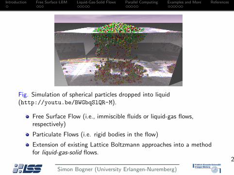
Fig. Simulation of spherical particles dropped into liquid(http://youtu.be/BWGbqSlQR-M).
Free Surface Flow (i.e., immiscible fluids or liquid-gas flows,respectively)
Particulate Flows (i.e. rigid bodies in the flow)
Extension of existing Lattice Boltzmann approaches into a methodfor liquid-gas-solid flows.
2
Simon Bogner (University Erlangen-Nuremberg)
Introduction Free Surface LBM Liquid-Gas-Solid Flows Parallel Computing Examples and More References
Outline1 Introduction
Lattice Boltzmann Model2 Free Surface LBM
Free Surface Extension3 Liquid-Gas-Solid Flows
Liquid-Solid Flows with LBMLiquid-Gas-Solid Flows with LBM
4 Parallel ComputingWaLBerla and MPIScaling results
5 Examples and MoreExample VideosConclusion
3
Simon Bogner (University Erlangen-Nuremberg)
Introduction Free Surface LBM Liquid-Gas-Solid Flows Parallel Computing Examples and More References
Table of Contents1 Introduction
Lattice Boltzmann Model2 Free Surface LBM
Free Surface Extension3 Liquid-Gas-Solid Flows
Liquid-Solid Flows with LBMLiquid-Gas-Solid Flows with LBM
4 Parallel ComputingWaLBerla and MPIScaling results
5 Examples and MoreExample VideosConclusion
4
Simon Bogner (University Erlangen-Nuremberg)
Introduction Free Surface LBM Liquid-Gas-Solid Flows Parallel Computing Examples and More References
Lattice and discrete velocities
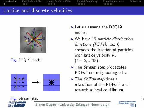
Fig. D3Q19 model
Fig. Stream step
Let us assume the D3Q19model.
We have 19 particle distributionfunctions (PDFs), i.e., fiencodes the fraction of particleswith lattice velocity vi ,(i = 0, .., 18).
The Stream step propagatesPDFs from neighboring cells.
The Collide step does arelaxation of the PDFs in a celltowards a local equilibrium.
5
Simon Bogner (University Erlangen-Nuremberg)
Introduction Free Surface LBM Liquid-Gas-Solid Flows Parallel Computing Examples and More References
Table of Contents1 Introduction
Lattice Boltzmann Model2 Free Surface LBM
Free Surface Extension3 Liquid-Gas-Solid Flows
Liquid-Solid Flows with LBMLiquid-Gas-Solid Flows with LBM
4 Parallel ComputingWaLBerla and MPIScaling results
5 Examples and MoreExample VideosConclusion
6
Simon Bogner (University Erlangen-Nuremberg)
Introduction Free Surface LBM Liquid-Gas-Solid Flows Parallel Computing Examples and More References
Basic Idea - Interface Tracking
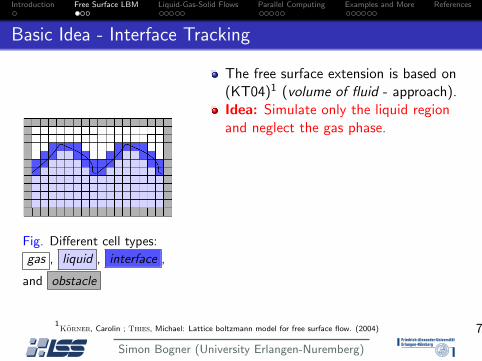
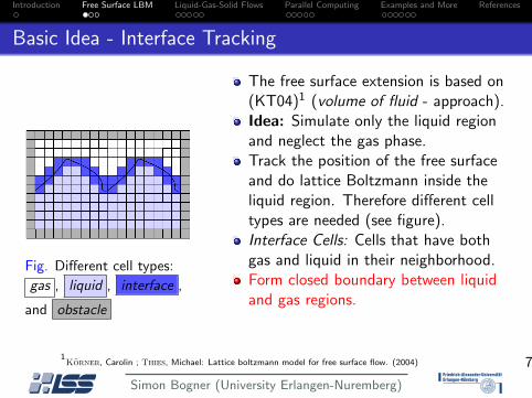
Fig. Different cell types:
gas , liquid , interface ,
and obstacle
The free surface extension is based on(KT04)1 (volume of fluid - approach).Idea: Simulate only the liquid regionand neglect the gas phase.
Track the position of the free surfaceand do lattice Boltzmann inside theliquid region. Therefore different celltypes are needed (see figure).Interface Cells: Cells that have bothgas and liquid in their neighborhood.Form closed boundary between liquidand gas regions.A free surface boundary conditionincorporates the gas pressure.
1Korner, Carolin ; Thies, Michael: Lattice boltzmann model for free surface flow. (2004) 7
Simon Bogner (University Erlangen-Nuremberg)
Introduction Free Surface LBM Liquid-Gas-Solid Flows Parallel Computing Examples and More References
Basic Idea - Interface Tracking
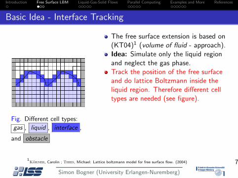
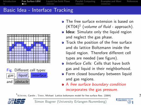
Fig. Different cell types:
gas , liquid , interface ,
and obstacle
The free surface extension is based on(KT04)1 (volume of fluid - approach).Idea: Simulate only the liquid regionand neglect the gas phase.Track the position of the free surfaceand do lattice Boltzmann inside theliquid region. Therefore different celltypes are needed (see figure).
Interface Cells: Cells that have bothgas and liquid in their neighborhood.Form closed boundary between liquidand gas regions.A free surface boundary conditionincorporates the gas pressure.
1Korner, Carolin ; Thies, Michael: Lattice boltzmann model for free surface flow. (2004) 7
Simon Bogner (University Erlangen-Nuremberg)
Introduction Free Surface LBM Liquid-Gas-Solid Flows Parallel Computing Examples and More References
Basic Idea - Interface Tracking
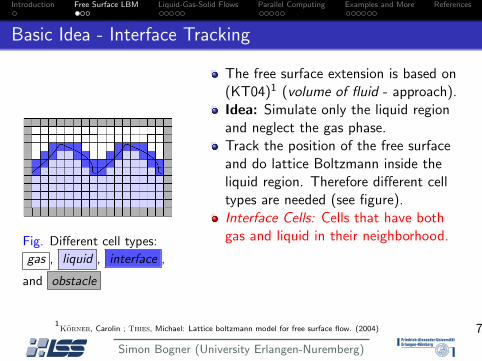
Fig. Different cell types:
gas , liquid , interface ,
and obstacle
The free surface extension is based on(KT04)1 (volume of fluid - approach).Idea: Simulate only the liquid regionand neglect the gas phase.Track the position of the free surfaceand do lattice Boltzmann inside theliquid region. Therefore different celltypes are needed (see figure).Interface Cells: Cells that have bothgas and liquid in their neighborhood.
Form closed boundary between liquidand gas regions.A free surface boundary conditionincorporates the gas pressure.
1Korner, Carolin ; Thies, Michael: Lattice boltzmann model for free surface flow. (2004) 7
Simon Bogner (University Erlangen-Nuremberg)
Introduction Free Surface LBM Liquid-Gas-Solid Flows Parallel Computing Examples and More References
Basic Idea - Interface Tracking
Fig. Different cell types:
gas , liquid , interface ,
and obstacle
The free surface extension is based on(KT04)1 (volume of fluid - approach).Idea: Simulate only the liquid regionand neglect the gas phase.Track the position of the free surfaceand do lattice Boltzmann inside theliquid region. Therefore different celltypes are needed (see figure).Interface Cells: Cells that have bothgas and liquid in their neighborhood.Form closed boundary between liquidand gas regions.
A free surface boundary conditionincorporates the gas pressure.
1Korner, Carolin ; Thies, Michael: Lattice boltzmann model for free surface flow. (2004) 7
Simon Bogner (University Erlangen-Nuremberg)
Introduction Free Surface LBM Liquid-Gas-Solid Flows Parallel Computing Examples and More References
Basic Idea - Interface Tracking
Fig. Different cell types:
gas , liquid , interface ,
and obstacle
The free surface extension is based on(KT04)1 (volume of fluid - approach).Idea: Simulate only the liquid regionand neglect the gas phase.Track the position of the free surfaceand do lattice Boltzmann inside theliquid region. Therefore different celltypes are needed (see figure).Interface Cells: Cells that have bothgas and liquid in their neighborhood.Form closed boundary between liquidand gas regions.A free surface boundary conditionincorporates the gas pressure.
1Korner, Carolin ; Thies, Michael: Lattice boltzmann model for free surface flow. (2004) 7
Simon Bogner (University Erlangen-Nuremberg)
Introduction Free Surface LBM Liquid-Gas-Solid Flows Parallel Computing Examples and More References
Interface Cells - Fill Levels
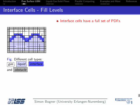
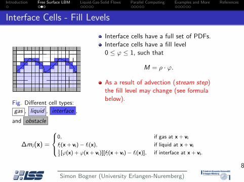
Fig. Different cell types:
gas , liquid , interface ,
and obstacle
Interface cells have a full set of PDFs.
Interface cells have a fill level0 ≤ ϕ ≤ 1, such that
M = ρ · ϕ.
As a result of advection (stream step)the fill level may change (see formulabelow).This mass tracking technique is thefirst step towards a dynamicalboundary.
∆mi (x) =
0, if gas at x + vi
fi (x + vi)− fi (x), if liquid at x + vi
12[ϕ(x) + ϕ(x + vi)][fi (x + vi)− fi (x)], if interface at x + vi.
8
Simon Bogner (University Erlangen-Nuremberg)
Introduction Free Surface LBM Liquid-Gas-Solid Flows Parallel Computing Examples and More References
Interface Cells - Fill Levels
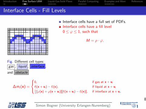
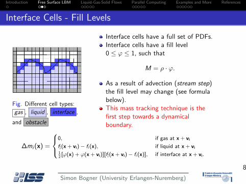
Fig. Different cell types:
gas , liquid , interface ,
and obstacle
Interface cells have a full set of PDFs.Interface cells have a fill level0 ≤ ϕ ≤ 1, such that
M = ρ · ϕ.
As a result of advection (stream step)the fill level may change (see formulabelow).This mass tracking technique is thefirst step towards a dynamicalboundary.
∆mi (x) =
0, if gas at x + vi
fi (x + vi)− fi (x), if liquid at x + vi
12[ϕ(x) + ϕ(x + vi)][fi (x + vi)− fi (x)], if interface at x + vi.
8
Simon Bogner (University Erlangen-Nuremberg)
Introduction Free Surface LBM Liquid-Gas-Solid Flows Parallel Computing Examples and More References
Interface Cells - Fill Levels
Fig. Different cell types:
gas , liquid , interface ,
and obstacle
Interface cells have a full set of PDFs.Interface cells have a fill level0 ≤ ϕ ≤ 1, such that
M = ρ · ϕ.
As a result of advection (stream step)the fill level may change (see formulabelow).
This mass tracking technique is thefirst step towards a dynamicalboundary.
∆mi (x) =
0, if gas at x + vi
fi (x + vi)− fi (x), if liquid at x + vi
12[ϕ(x) + ϕ(x + vi)][fi (x + vi)− fi (x)], if interface at x + vi.
8
Simon Bogner (University Erlangen-Nuremberg)
Introduction Free Surface LBM Liquid-Gas-Solid Flows Parallel Computing Examples and More References
Interface Cells - Fill Levels
Fig. Different cell types:
gas , liquid , interface ,
and obstacle
Interface cells have a full set of PDFs.Interface cells have a fill level0 ≤ ϕ ≤ 1, such that
M = ρ · ϕ.
As a result of advection (stream step)the fill level may change (see formulabelow).This mass tracking technique is thefirst step towards a dynamicalboundary.
∆mi (x) =
0, if gas at x + vi
fi (x + vi)− fi (x), if liquid at x + vi
12[ϕ(x) + ϕ(x + vi)][fi (x + vi)− fi (x)], if interface at x + vi.
8
Simon Bogner (University Erlangen-Nuremberg)
Introduction Free Surface LBM Liquid-Gas-Solid Flows Parallel Computing Examples and More References
Interface Cells - Cell Conversion
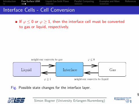
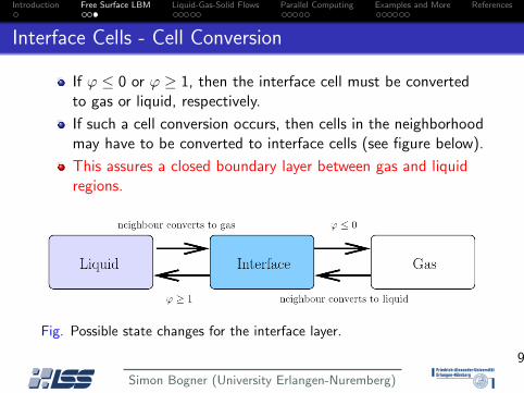
If ϕ ≤ 0 or ϕ ≥ 1, then the interface cell must be convertedto gas or liquid, respectively.
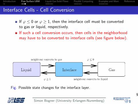
If such a cell conversion occurs, then cells in the neighborhoodmay have to be converted to interface cells (see figure below).
This assures a closed boundary layer between gas and liquidregions.
Fig. Possible state changes for the interface layer.
9
Simon Bogner (University Erlangen-Nuremberg)
Introduction Free Surface LBM Liquid-Gas-Solid Flows Parallel Computing Examples and More References
Interface Cells - Cell Conversion
If ϕ ≤ 0 or ϕ ≥ 1, then the interface cell must be convertedto gas or liquid, respectively.
If such a cell conversion occurs, then cells in the neighborhoodmay have to be converted to interface cells (see figure below).
This assures a closed boundary layer between gas and liquidregions.
Fig. Possible state changes for the interface layer.
9
Simon Bogner (University Erlangen-Nuremberg)

Introduction Free Surface LBM Liquid-Gas-Solid Flows Parallel Computing Examples and More References
Table of Contents1 Introduction
Lattice Boltzmann Model2 Free Surface LBM
Free Surface Extension3 Liquid-Gas-Solid Flows
Liquid-Solid Flows with LBMLiquid-Gas-Solid Flows with LBM
4 Parallel ComputingWaLBerla and MPIScaling results
5 Examples and MoreExample VideosConclusion
10
Simon Bogner (University Erlangen-Nuremberg)

Introduction Free Surface LBM Liquid-Gas-Solid Flows Parallel Computing Examples and More References
Liquid-Solid Flows with LBM
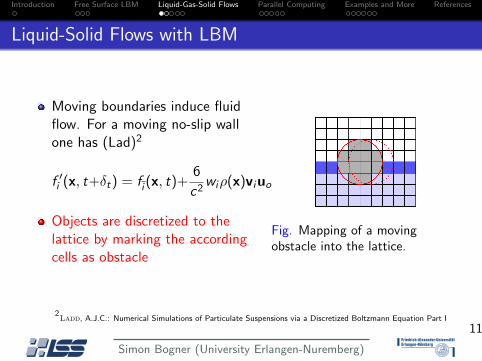
Moving boundaries induce fluidflow. For a moving no-slip wallone has (Lad)2
f ′i (x, t+δt) = fi (x, t)+
6
c2wiρ(x)viuo
Objects are discretized to thelattice by marking the accordingcells as obstacle
Fig. Mapping of a movingobstacle into the lattice.
2Ladd, A.J.C.: Numerical Simulations of Particulate Suspensions via a Discretized Boltzmann Equation Part I
11
Simon Bogner (University Erlangen-Nuremberg)
Introduction Free Surface LBM Liquid-Gas-Solid Flows Parallel Computing Examples and More References
Liquid-Solid Flows with LBM
Moving boundaries induce fluidflow. For a moving no-slip wallone has (Lad)2
f ′i (x, t+δt) = fi (x, t)+
6
c2wiρ(x)viuo
Objects are discretized to thelattice by marking the accordingcells as obstacle
Fig. Mapping of a movingobstacle into the lattice.
2Ladd, A.J.C.: Numerical Simulations of Particulate Suspensions via a Discretized Boltzmann Equation Part I
11
Simon Bogner (University Erlangen-Nuremberg)

Introduction Free Surface LBM Liquid-Gas-Solid Flows Parallel Computing Examples and More References
Momentum Exchange Method
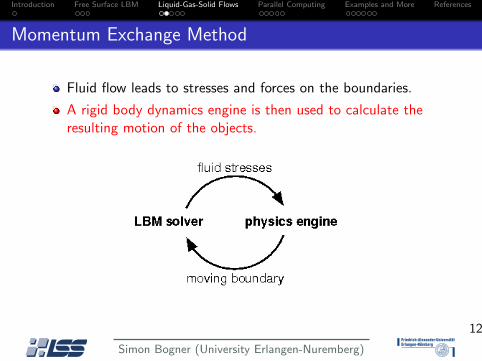
Fluid flow leads to stresses and forces on the boundaries.
A rigid body dynamics engine is then used to calculate theresulting motion of the objects.
12
Simon Bogner (University Erlangen-Nuremberg)
Introduction Free Surface LBM Liquid-Gas-Solid Flows Parallel Computing Examples and More References
Momentum Exchange Method
Fluid flow leads to stresses and forces on the boundaries.
A rigid body dynamics engine is then used to calculate theresulting motion of the objects.
12
Simon Bogner (University Erlangen-Nuremberg)
Introduction Free Surface LBM Liquid-Gas-Solid Flows Parallel Computing Examples and More References
Liquid-Gas-Solid Flows
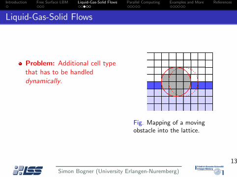
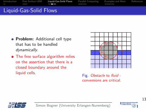
Problem: Additional cell typethat has to be handleddynamically.
The free surface algorithm relieson the assertion that there is aclosed boundary around theliquid cells.
Fig. Mapping of a movingobstacle into the lattice.
13
Simon Bogner (University Erlangen-Nuremberg)
Introduction Free Surface LBM Liquid-Gas-Solid Flows Parallel Computing Examples and More References
Liquid-Gas-Solid Flows
Problem: Additional cell typethat has to be handleddynamically.
The free surface algorithm relieson the assertion that there is aclosed boundary around theliquid cells.
Fig. Obstacle to fluid -conversions are critical.
13
Simon Bogner (University Erlangen-Nuremberg)
Introduction Free Surface LBM Liquid-Gas-Solid Flows Parallel Computing Examples and More References
Complex Cell Conversion Algorithm
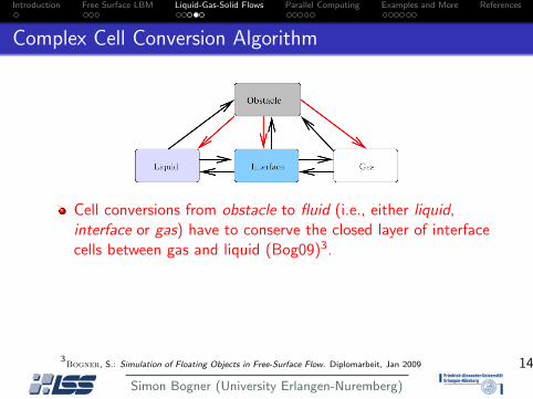
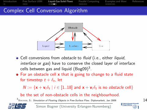
Cell conversions from obstacle to fluid (i.e., either liquid,interface or gas) have to conserve the closed layer of interfacecells between gas and liquid (Bog09)3.
For an obstacle cell x that is going to change to a fluid statefor timestep t + δt , let
N := {x + viδt | i ∈ [1..18] and x + viδt is no obstacle cell}be the set of non-obstacle cells in the neighbourhood.
3Bogner, S.: Simulation of Floating Objects in Free-Surface Flow. Diplomarbeit, Jan 2009 14
Simon Bogner (University Erlangen-Nuremberg)
Introduction Free Surface LBM Liquid-Gas-Solid Flows Parallel Computing Examples and More References
Complex Cell Conversion Algorithm
Cell conversions from obstacle to fluid (i.e., either liquid,interface or gas) have to conserve the closed layer of interfacecells between gas and liquid (Bog09)3.For an obstacle cell x that is going to change to a fluid statefor timestep t + δt , let
N := {x + viδt | i ∈ [1..18] and x + viδt is no obstacle cell}be the set of non-obstacle cells in the neighbourhood.
3Bogner, S.: Simulation of Floating Objects in Free-Surface Flow. Diplomarbeit, Jan 2009 14
Simon Bogner (University Erlangen-Nuremberg)
Introduction Free Surface LBM Liquid-Gas-Solid Flows Parallel Computing Examples and More References
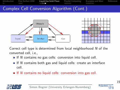
Complex Cell Conversion Algorithm (Cont.)
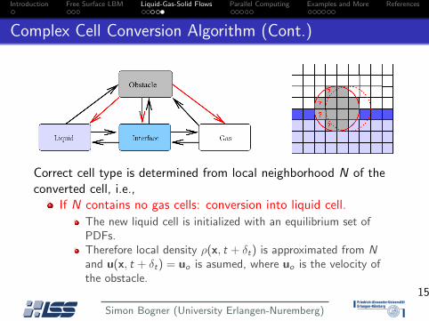
Correct cell type is determined from local neighborhood N of theconverted cell, i.e.,
If N contains no gas cells: conversion into liquid cell.
The new liquid cell is initialized with an equilibrium set ofPDFs.Therefore local density ρ(x, t + δt) is approximated from Nand u(x, t + δt) = uo is asumed, where uo is the velocity ofthe obstacle.
If N contains both gas and liquid cells: create an interfacecell.
If N contains no liquid cells: conversion into gas cell.
15
Simon Bogner (University Erlangen-Nuremberg)

Introduction Free Surface LBM Liquid-Gas-Solid Flows Parallel Computing Examples and More References
Complex Cell Conversion Algorithm (Cont.)
Correct cell type is determined from local neighborhood N of theconverted cell, i.e.,
If N contains no gas cells: conversion into liquid cell.
If N contains both gas and liquid cells: create an interfacecell.
PDFs are set to equilibrium as for liquid cells.In addition to the PDFs, a fill value has to be interpolatedfrom the neighborhood N.
If N contains no liquid cells: conversion into gas cell.
15
Simon Bogner (University Erlangen-Nuremberg)
Introduction Free Surface LBM Liquid-Gas-Solid Flows Parallel Computing Examples and More References
Complex Cell Conversion Algorithm (Cont.)
Correct cell type is determined from local neighborhood N of theconverted cell, i.e.,
If N contains no gas cells: conversion into liquid cell.
If N contains both gas and liquid cells: create an interfacecell.
If N contains no liquid cells: conversion into gas cell.
15
Simon Bogner (University Erlangen-Nuremberg)
Introduction Free Surface LBM Liquid-Gas-Solid Flows Parallel Computing Examples and More References
Table of Contents1 Introduction
Lattice Boltzmann Model2 Free Surface LBM
Free Surface Extension3 Liquid-Gas-Solid Flows
Liquid-Solid Flows with LBMLiquid-Gas-Solid Flows with LBM
4 Parallel ComputingWaLBerla and MPIScaling results
5 Examples and MoreExample VideosConclusion
16
Simon Bogner (University Erlangen-Nuremberg)
Introduction Free Surface LBM Liquid-Gas-Solid Flows Parallel Computing Examples and More References
WaLBerla Communication Concept
WaLBerla framework: Widely applicable Lattice Boltzmannsoftware framework from Erlangen.
Simulation domain is split into patches, which are thendistributed over the number of processes.Ghostlayer concept.If neighboring patches are residing on different processes, thenthe patch data is communicated via MPI.
Fig. WaLBerla logo, see http://www10.informatik.uni-erlangen.de/Research/Projects/walberla/.
17
Simon Bogner (University Erlangen-Nuremberg)

Introduction Free Surface LBM Liquid-Gas-Solid Flows Parallel Computing Examples and More References
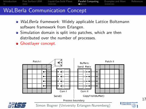
WaLBerla Communication Concept
WaLBerla framework: Widely applicable Lattice Boltzmannsoftware framework from Erlangen.Simulation domain is split into patches, which are thendistributed over the number of processes.
Ghostlayer concept.If neighboring patches are residing on different processes, thenthe patch data is communicated via MPI.
17
Simon Bogner (University Erlangen-Nuremberg)
Introduction Free Surface LBM Liquid-Gas-Solid Flows Parallel Computing Examples and More References
WaLBerla Communication Concept
WaLBerla framework: Widely applicable Lattice Boltzmannsoftware framework from Erlangen.Simulation domain is split into patches, which are thendistributed over the number of processes.Ghostlayer concept.
If neighboring patches are residing on different processes, thenthe patch data is communicated via MPI.
17
Simon Bogner (University Erlangen-Nuremberg)

Introduction Free Surface LBM Liquid-Gas-Solid Flows Parallel Computing Examples and More References
WaLBerla Communication Concept
WaLBerla framework: Widely applicable Lattice Boltzmannsoftware framework from Erlangen.Simulation domain is split into patches, which are thendistributed over the number of processes.Ghostlayer concept.If neighboring patches are residing on different processes, thenthe patch data is communicated via MPI.
17
Simon Bogner (University Erlangen-Nuremberg)
Introduction Free Surface LBM Liquid-Gas-Solid Flows Parallel Computing Examples and More References
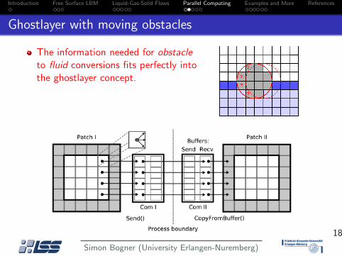
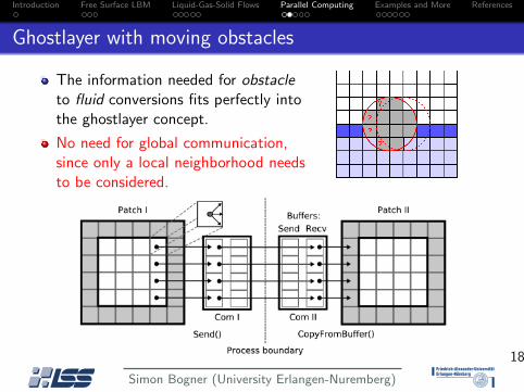
Ghostlayer with moving obstacles
The information needed for obstacleto fluid conversions fits perfectly intothe ghostlayer concept.
No need for global communication,since only a local neighborhood needsto be considered.
18
Simon Bogner (University Erlangen-Nuremberg)
Introduction Free Surface LBM Liquid-Gas-Solid Flows Parallel Computing Examples and More References
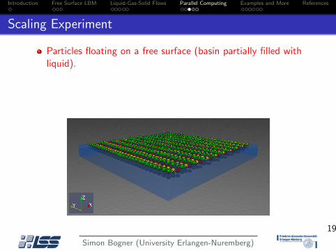
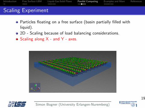
Scaling Experiment
Particles floating on a free surface (basin partially filled withliquid).
2D - Scaling because of load balancing considerations.
Scaling along X - and Y - axes.
LIMA Cluster, RRZE http://www.rrze.uni-erlangen.de
19
Simon Bogner (University Erlangen-Nuremberg)
Introduction Free Surface LBM Liquid-Gas-Solid Flows Parallel Computing Examples and More References
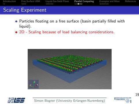
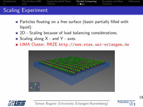
Scaling Experiment
Particles floating on a free surface (basin partially filled withliquid).
2D - Scaling because of load balancing considerations.
Scaling along X - and Y - axes.
LIMA Cluster, RRZE http://www.rrze.uni-erlangen.de
19
Simon Bogner (University Erlangen-Nuremberg)
Introduction Free Surface LBM Liquid-Gas-Solid Flows Parallel Computing Examples and More References
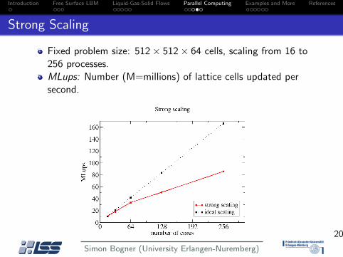
Strong Scaling
Fixed problem size: 512× 512× 64 cells, scaling from 16 to256 processes.MLups: Number (M=millions) of lattice cells updated persecond.
20
Simon Bogner (University Erlangen-Nuremberg)

Introduction Free Surface LBM Liquid-Gas-Solid Flows Parallel Computing Examples and More References
Weak Scaling
Scaling the problem size, from 320× 240× 300 cells on 24processes to: 2560× 1920× 300 cells on 1536 processes.Performance was 998 MLups (i.e., 86% performancecompared to ideal scaling).
21
Simon Bogner (University Erlangen-Nuremberg)
Introduction Free Surface LBM Liquid-Gas-Solid Flows Parallel Computing Examples and More References
Table of Contents1 Introduction
Lattice Boltzmann Model2 Free Surface LBM
Free Surface Extension3 Liquid-Gas-Solid Flows
Liquid-Solid Flows with LBMLiquid-Gas-Solid Flows with LBM
4 Parallel ComputingWaLBerla and MPIScaling results
5 Examples and MoreExample VideosConclusion
22
Simon Bogner (University Erlangen-Nuremberg)
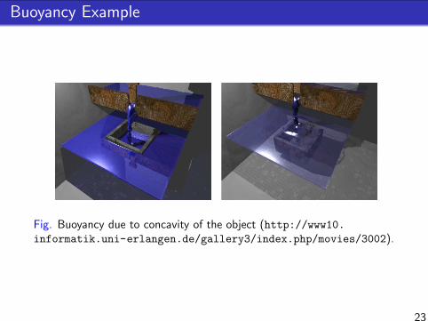
Buoyancy Example
Fig. Buoyancy due to concavity of the object (http://www10.informatik.uni-erlangen.de/gallery3/index.php/movies/3002).
23
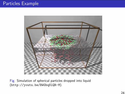
Particles Example
Fig. Simulation of spherical particles dropped into liquid(http://youtu.be/BWGbqSlQR-M).
24
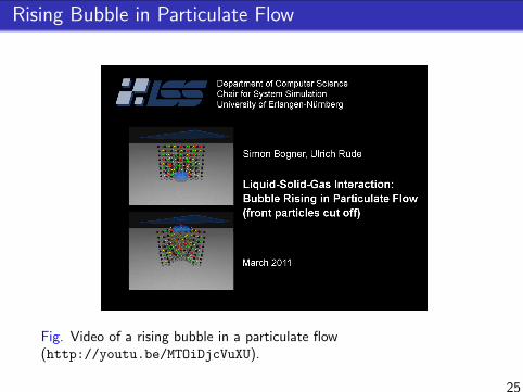
Rising Bubble in Particulate Flow
Fig. Video of a rising bubble in a particulate flow(http://youtu.be/MTOiDjcVuXU).
25
Introduction Free Surface LBM Liquid-Gas-Solid Flows Parallel Computing Examples and More References
Conclusion
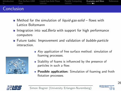
Method for the simulation of liquid-gas-solid – flows withLattice Boltzmann
Integration into waLBerla with support for high performancecomputers
Future tasks: Improvement and validation of bubble-particleinteraction.
Key application of free surface method: simulation offoaming processes.
Stability of foams is influenced by the presence ofparticles in such a flow.
Possible application: Simulation of foaming and frothflotation processes.
26
Simon Bogner (University Erlangen-Nuremberg)
Introduction Free Surface LBM Liquid-Gas-Solid Flows Parallel Computing Examples and More References
Conclusion
Method for the simulation of liquid-gas-solid – flows withLattice Boltzmann
Integration into waLBerla with support for high performancecomputers
Future tasks: Improvement and validation of bubble-particleinteraction.
Key application of free surface method: simulation offoaming processes.
Stability of foams is influenced by the presence ofparticles in such a flow.
Possible application: Simulation of foaming and frothflotation processes.
26
Simon Bogner (University Erlangen-Nuremberg)
Introduction Free Surface LBM Liquid-Gas-Solid Flows Parallel Computing Examples and More References
Thank you very much for listening!
http://www10.informatik.uni-erlangen.de
27
Simon Bogner (University Erlangen-Nuremberg)
References
[Bog09] Bogner, S.: Simulation of Floating Objects inFree-Surface Flow. Diplomarbeit, Jan 2009
[KT04] Korner, Carolin ; Thies, Michael: Lattice boltzmannmodel for free surface flow. (2004)
[Lad] Ladd, A.J.C.: Numerical Simulations of ParticulateSuspensions via a Discretized Boltzmann Equation Part I.
28