simulation of laser additive manufacturing and its ... · simulation of laser additive...
TRANSCRIPT

Simulation of Laser Additive Manufacturing and its Applications
DISSERTATION
Presented in Partial Fulfillment of the Requirements for the Degree Doctor of Philosophy
in the Graduate School of The Ohio State University
By
Yousub Lee
Graduate Program in Welding Engineering
The Ohio State University
2015
Dissertation Committee:
Professor Dave F. Farson, Advisor
Professor Wei Zhang, Advisor
Professor Antonio J. Ramirez

Copyright by
Yousub Lee
2015
ii
Abstract
Laser and metal powder based additive manufacturing (AM), a key category of
advanced Direct Digital Manufacturing (DDM), produces metallic components directly
from a digital representation of the part such as a CAD file. It is well suited for the
production of high-value, customizable components with complex geometry and the
repair of damaged components.
Currently, the main challenges for laser and metal powder based AM include the
formation of defects (e.g., porosity), low surface finish quality, and spatially non-uniform
properties of material. Such challenges stem largely from the limited knowledge of
complex physical processes in AM especially the molten pool physics such as melting,
molten metal flow, heat conduction, vaporization of alloying elements, and solidification.
Direct experimental measurement of melt pool phenomena is highly difficult since the
process is localized (on the order of 0.1 mm to 1 mm melt pool size) and transient (on the
order of 1 m/s scanning speed). Furthermore, current optical and infrared cameras are
limited to observe the melt pool surface. As a result, fluid flows in the melt pool, melt
pool shape and formation of sub-surface defects are difficult to be visualized by
experiment. On the other hand, numerical simulation, based on rigorous solution of mass,

iii
momentum and energy transport equations, can provide important quantitative
knowledge of complex transport phenomena taking place in AM.
The overarching goal of this dissertation research is to develop an analytical
foundation for fundamental understanding of heat transfer, molten metal flow and free
surface evolution. Two key types of laser AM processes are studied: a) powder injection,
commonly used for repairing of turbine blades, and b) powder bed, commonly used for
manufacturing of new parts with complex geometry.
In the powder injection simulation, fluid convection, temperature gradient (G),
solidification rate (R) and melt pool shape are calculated using a heat transfer and fluid
flow model, which solves the mass, momentum and energy transport equations using the
volume of fluid (VOF) method. These results provide quantitative understanding of
underlying mechanisms of solidification morphology, solidification scale and deposit side
bulging. In particular, it is shown that convective mixing alters solidification conditions
(G and R), cooling trend and resultant size of primary dendrite arm spacing. Melt pool
convexity in multiple layer LAM is associated not only with the convex shape of prior
deposit but also with Marangoni flow. Lastly, it is shown that the lateral width of bulge is
possibly controlled by the type of surface tension gradient.
It is noted that laser beam spot size in the powder injection AM is about 2 mm
and it melts hundreds of powder particles. Hence, the injection of individual particles is
approximated by a lumped mass flux into the molten pool. On the other hand, for laser
powder bed AM, the laser beam spot size is about 100 μm and thus it only melts a few
iv
tens of particles. Therefore, resolution of individual powder particles is essential for the
accurate simulation of laser powder bed AM.
To obtain the powder packing information in the powder bed, dynamic discrete
element simulation (DEM) is used. It considers particle-particle interactions during
packing to provide the quantitative structural powder bed properties such as particle
arrangement, size and packing density, which is then an inputted as initial geometry for
heat transfer and fluid flow simulation. This coupled 3D transient transport model
provides a high spatial resolution while requiring less demanding computation. The
results show that negatively skewed particle size distribution, faster scanning speed, low
power and low packing density worsen the surface finish quality and promote the
formation of balling defects.
Taken together, both powder injection and powder bed models have resulted in an
improved quantitative understanding of heat transfer, molten metal flow and free surface
evolution. Furthermore, the analytical foundation that is developed in this dissertation
provides the temperature history in AM, a prerequisite for predicting the solid-state phase
transformation kinetics, residual stresses and distortion using other models. Moreover, it
can be integrated with experimental monitoring and sensing tools to provide the
capability of controlling melt pool shape, solidification microstructure, defect formation
and surface finish.

v
Dedicated to my parents and wife

vi
Acknowledgments
I would like to greatly appreciate my advisor, Prof. Dave Farson for his guidance,
valuable advice and support throughout my PhD studies at The Ohio State University. As
a professor, Dr. Farson is one of the distinctive researchers in the welding engineering
and laser materials processing. He is actively serving technical societies as President,
Board Member and other offices for Laser Institute of America. As my advisor, he has
pleasantly helped me all the time with big patience to correct my scientific mistakes.
I must thank to my co-advisor, Prof. Wei Zhang for his smart advices,
encouragement and support for the last year of my PhD study. Before he came to OSU as
a professor, he was a distinctive researcher at Oak Ridge National Laboratory (ORNL)
and Edison Welding Institute (EWI). He is now a core faculty for Simulation Innovation
and Modeling Center (SIMCenter). Being his student, I have learned critical thinking and
writing making me an independent researcher. Moreover, I realize that he is always ready
to help his students to achieve academic and career goals.
Also, I truly thank Prof. Suresh Babu at University of Tennessee, Knoxville for
his enthusiastic comments and help during my graduate school. I would like to thank
Prof. Antonio Ramirez being a committee member and his critical comments on my
dissertation.

vii
I would like to acknowledge Rolls Royce, CIMJSEA center (Now, Ma2JIC) and
Office of Naval Research for the financial support. I appreciate Dr. J.S. Bader and M.
Nordin (Rolls Royce), Prof. John Lippold (CIMJSEA) and Dr. Richard W. Fonda (ORN).
Thanks to all my colleagues and professors in WE and MSE for all helps.
Last but not least, thanks to my parents and younger sister for their unbelievable
support and love. Special thanks to my wife, Jinmo. I will always remember your endless
patience and love.

viii
Vita
1979................................................................Born-Daegu, South Korea
2007................................................................B.S. Materials Science and Metallurgical
Engineering, Kyungpook National University
2009................................................................M.S. Materials Science and Engineering,
Seoul National University
2011 to present ..............................................Graduate Research Associate, Welding
Engineering, The Ohio State University
Publications
1. Lee YS, Nordin M, Babu SS, Farson DF (2014) Influence of fluid convection on weld
pool formation in laser cladding. Welding Journal 93(8):292S-300S.
2. Lee Y, Nordin M, Babu SS, Farson DF (2014) Effect of Fluid Convection on Dendrite
Arm Spacing in Laser Deposition. Metallurgical and Materials Transactions B 45(4):
1520-1529.
3. Lee YS and Zhang W Mesoscopic (2015) Simulation of Heat Transfer and Fluid Flow
in Laser Powder Bed Fusion Additive Manufacturing. In Proceeding of Solid Freeform
Fabrication Symposium, Austin, Texas

ix
Fields of Study
Major Field: Welding Engineering

x
Table of Contents
Abstract ............................................................................................................................... ii
Acknowledgments.............................................................................................................. vi
Vita ................................................................................................................................... viii
Table of Contents ................................................................................................................ x
List of Tables ................................................................................................................... xiv
List of Figures ................................................................................................................... xv
Chapter 1: Introduction ....................................................................................................... 1
Chapter 2: Influence of Fluid Convection on Weld Pool Formation in Laser Cladding .... 9
2.1 Introduction ............................................................................................................... 9
2.2 Experimental Conditions ......................................................................................... 12
2.3 Clad deposit modeling ............................................................................................. 13
2.3.1 Governing equations ......................................................................................... 14
2.3.2 Boundary conditions and physical properties for the simulation ..................... 16
2.4 Laser Cladding Process Mechanisms and Models .................................................. 19
2.4.1 Absorptance of laser beam energy .................................................................... 20
2.4.2 Energy balance ................................................................................................. 21
2.5 Results and discussion ............................................................................................. 28
2.5.1 Powder catchment efficiency ............................................................................ 28
2.5.2 Melt pool size: experiment vs. simulation ........................................................ 29
2.5.3 Fluid flow patterns in melt pool ....................................................................... 31
2.6 Summary, conclusions and future work .................................................................. 37
2.7 Acknowledgement ................................................................................................... 38

xi
2.8 References ............................................................................................................... 39
Chapter 3: Effect of Fluid Convection on Dendrite Arm Spacing in Laser Deposition ... 42
3.1 Introduction ............................................................................................................. 42
3.1.1 Fluid Dynamics and its effect on weld pool shape ........................................... 44
3.1.2 Correlation of the weld pool shape with solidification microstructure ............ 46
3.2 Flow and Solidification Model ................................................................................ 49
3.2.1 Weld pool shape and solidification conditions ................................................. 49
3.2.2 Temperature gradient and solidification rate .................................................... 52
3.2.3 Solidification Microstructure Models ............................................................... 54
3.3 Experimental ........................................................................................................... 55
3.4 Numerical Model Results and Solidification Microstructure Prediction ................ 56
3.5. Summary and Conclusions ..................................................................................... 64
3.6 Acknowledgements ................................................................................................. 65
3.7 Nomenclature .......................................................................................................... 65
3.8 References ............................................................................................................... 67
Chapter 4: Simulation of Transport Phenomena and Melt Pool Shape for Multiple Layer
Additive Manufacturing .................................................................................................... 71
4.1 Introduction ............................................................................................................. 71
4.2 Physical model ........................................................................................................ 74
4.2.1 Fundamental equations ..................................................................................... 74
4.2.2 Boundary conditions ......................................................................................... 75
4.2.3 Process heat and mass transfer efficiencies ...................................................... 79
4.3 Results and discussion ............................................................................................. 82
4.4 Summary and conclusion ........................................................................................ 93
4.5 Acknowledgements ................................................................................................. 94
4.6 References ............................................................................................................... 95
Chapter 5: Surface Tension-Powered Surface Finish Control in Laser Additive
Manufacturing Process...................................................................................................... 98

xii
5.1 Introduction ............................................................................................................. 98
5.2 Physical model ...................................................................................................... 103
5.2.1 Governing equations ....................................................................................... 103
5.2.2 Boundary conditions and physical properties ................................................. 104
5.3 Result and discussion ............................................................................................ 109
5.4 Summary and conclusion ...................................................................................... 119
5.5 Acknowledgements ............................................................................................... 120
5.6 References ............................................................................................................. 120
Chapter 6: Random Particle Packing Simulation with Asymmetric Size Distribution for
Laser Powder Bed Additive Manufacturing ................................................................... 124
6.1 Introduction ........................................................................................................... 124
6.2 Nature of Discrete Element Method ...................................................................... 126
6.2.1 Description of Calculation Procedure and Assumptions ................................ 126
6.2.2 Algorithms of DEM simulation.......................................................................... 127
6.3. Result and Discussion .......................................................................................... 132
6.4 Summary and conclusions ..................................................................................... 142
6.5 Acknowledgement ................................................................................................. 144
6.6 References ............................................................................................................. 144
Chapter 7: Mesoscopic Simulation of Heat Transfer and Fluid Flow in Laser Powder Bed
Additive Manufacturing .................................................................................................. 147
7.1 Introduction ........................................................................................................... 147
7.2 Numerical modeling approach .............................................................................. 149
7.2.1. Discrete element method simulation of powder packing .............................. 149
7.2.2 Governing equations for heat transfer and fluid flow ..................................... 152
7.2.3 Computational domain, boundary conditions and materials properties ......... 154
7.3 Result and discussion ............................................................................................ 157
7.3.1 Stack-up of powder particles with different PSDs ......................................... 157
7.3.2 Fluid flow and molten pool shape .................................................................. 158

xiii
7.3.3 Formation of balling defect ............................................................................ 160
7.4 Summary and conclusion ...................................................................................... 167
7.5 Acknowledgements ............................................................................................... 168
7.6 References ............................................................................................................. 168
Chapter 8: Conclusion and future work .......................................................................... 171
Bibliography ................................................................................................................... 176

xiv
List of Tables
Table 2.1 Nominal composition of IN718 Powder in weight percent .............................. 13
Table 2.2 Thermophysical properties of IN718 and process parameters used in numerical
model................................................................................................................................. 18
Table 2.3 Calculation of catchment efficiency ................................................................. 29
Table 3.1 Physical properties of nickel based superalloy used in theoretical prediction . 55
Table 4.1 Thermophysical properties of IN718 powder and substrate and process
parameters used in this simulation .................................................................................... 77
Table 4.2 Parameters used for heat balance calculation ................................................... 80
Table 5.1 Thermophysical properties and manufacturing parameters used in simulation
[20,21,24,25] ................................................................................................................... 109
Table 6.1 Process conditions for particle packing simulation ........................................ 132
Table 6.2 Correlation of packing density with D90/D10 ratio .......................................... 142
Table 7.1 Additional thermos-physical properties of IN718 and L-PBF processing
parameters. ...................................................................................................................... 156

xv
List of Figures
Figure 1.1 Schematic of two types of laser additive manufacturing (LAM) (a) powder
injection system (b) powder bed system ............................................................................. 2
Figure 1.2 Research objectives of this dissertation ............................................................. 4
Figure 2.1 Schematic of laser cladding process using coaxial powder feed nozzle ......... 10
Figure 2.2 Boundary conditions for the edges of substrate and powder nozzle and (a) and
description of computation domain (b) ............................................................................. 18
Figure 2.3 Energy balance during laser cladding process................................................. 22
Figure 2.4 Distribution of laser energy in the laser cladding process ............................... 23
Figure 2.5 Assumption for powder catchment efficiency ................................................. 25
Figure 2.6 The temperature and surface active element dependent values of surface
tension ............................................................................................................................... 26
Figure 2.7 Effect of G and R on solidification morphology ............................................. 27
Figure 2.8 Top-down (a) and cross section (b) views at the same magnification for
comparison of simulated and experimental single pass laser clad melt pool and deposits at
various powers. Dashed lines in simulation images show the position of liquidus isotherm
while dashed lines in experimental images show the liquidus isotherm from the
corresponding simulation .................................................................................................. 30
Figure 2.9 Comparison of simulated and experimental weld pool dimensions ................ 30
Figure 2.10 Quasi-steady state temperature profile and temperature gradient (G) along the
weld pool centerline at time t=0.43s ................................................................................. 32

xvi
Figure 2.11 Longitudinal-section view showing fluid flow and mixing in the laser clad
melt pool, the location of laser focus spot. The green dot indicates the location of the
weld pool surface with temperature Ti where surface tension gradient transitions from
positive to negative. .......................................................................................................... 33
Figure 2.12 Three dimensional depiction of weld pool convection flows (c) with inset
figures showing temperature-dependent surface tension (a) and surface temperature (b).
In (a), surface tension gradient switches from positive to negative at Ti. In (b), Ti
separates the positive (blue) and negative (red) surface tension regions. The two opposing
surface flows impinge along the line where surface temperature equals Ti. .................... 35
Figure 2.13 3D and 2D plots showing fluid flow and mixing in laser clad melt pool ...... 36
Figure 3.1 Different fluid flow pattern produced by different surface tension gradient ... 45
Figure 3.2 The effect of G and R on the solidification morphology and size ................... 47
Figure 3.3 Measured primary dendrite arm spacing from a single layer clad deposit ...... 56
Figure 3.4 Solidification rate R calculated on the weld pool solidification boundary. The
small inset graphic on the lower left shows the location of the points on a 3-D graphic of
the solidification boundary at the rear edge of the weld pool (due to half-symmetry, only
½ of the solidification boundary is shown). ...................................................................... 57
Figure 3.5 Temperature gradient G calculated on the weld pool boundary ...................... 58
Figure 3.6 Cooling rate predicted by the product G R on the weld pool boundary. The
cooling rate at height A increases as one traverses along the solidification boundary from
the weld centerline toward the point of maximum weld, but then reaches maximum and
suddenly decreases in a narrow region near the maximum pool width. At a deeper depth
B, the cooling rate increases from when traversing along the solidification boundary from
weld centerline but reaches a maximum and begins to decrease at point closer to the
trailing edge than at depth A. At deepest depth C, the maximum cooling rate is at the
weld centerline and cooling rate only decreases when traversing along the solidification
boundary toward the maximum pool width. ..................................................................... 60

xvii
Figure 3.7 Solidification boundary cooling rate, location of maximum cooling rate and
fluid flow pattern at heights A, B and C. Marangoni convection causes somewhat lower
maximum boundary cooling rate near the point of widest pool width on the top surface
of the weld pool (depth A). The maximum cooling is larger at depth C and its location
shifts rearward towards the trailing weld pool edge. Red arrows: fluid flow direction in
the weld pool liquid; Green dashed arrows: focus on fluid flow direction adjacent to
solidification boundary that causes reversal in cooling rate, in the mixing zone; Black
solid arrows: indicates a backward shift in maximum cooling rate to solidification
boundary locations closer to the bottom and center of the weld pool. ............................. 62
Figure 3.8 PDAS along weld pool solidification boundary predicted using Kurz-Fisher
and Trivedi models at three Z-axis heights A, B and C, respectively. Weld center is at the
middle of the back edge of the weld pool at Y=0 and X=0.275 and weld edge denotes the
location of maximum weld width. The grey shaded area corresponds to solidification
boundary located influenced by the weld pool convection mixing zone. ......................... 63
Figure 4.1 Initial setting of computational domain ........................................................... 75
Figure 4.2 Variation of width and height of the 5 layer deposit with change of surface
tension gradient from positive to negative to mixed ......................................................... 78
Figure 4.3 Simulation results showing melt pool at the midpoint of five deposition layers:
(a) first layer, (b) second layer, (c) third layer, (d) fourth layer, and (e) fifth layer ......... 83
Figure 4.4 Thermal cycles at a mid-length, mid-width point on the deposit surface for five
layers ................................................................................................................................. 85
Figure 4.5 Build profile and evolution shown by overlapped profiles from the mid-length
of a five-layer deposit: (a) cross section and (b) profile, fusion boundary and remelting of
successive layers ............................................................................................................... 85
Figure 4.6 Comparison of simulation predictions and experimental measurements [20] at
mid-length of a five-layer deposit: (a) height and width, (b) peak temperature for each
layer................................................................................................................................... 87
Figure 4.7 Progression of convexity at weld pool bottom through 1st to 5th layer in the
transverse cross-sections at the mid-center of the deposit from each layer ...................... 88

xviii
Figure 4.8 Comparison of fluid flow patterns in laser welding (a) and LAM (b) ............ 89
Figure 4.9 Transition of fluid flow pattern and surface flow velocity direction at the mid-
length of the deposit. As the deposit height increases, the downward surface flow at the
outer edge produces a convex weld pool bottom shape: (a) 1st layer, (b) 3rd layer, and (c)
5th layer ............................................................................................................................. 91
Figure 5.1 Different fluid flow pattern and melt pool shapes produced by different
directions of thermocapillary gradient: (a) negative, (b) positive and (c) mixed gradient
......................................................................................................................................... 102
Figure 5.2 Surface tension–temperature gradients used in the simulations: negative,
positive, mixed at 6 ppm and 10 ppm sulfur ................................................................... 107
Figure 5.3 Schematic description of computation domain ............................................. 108
Figure 5.4 Effect of thermocapillary gradients on deposit geometry at the starting position
......................................................................................................................................... 111
Figure 5.5 Measurement of simulated deposit widths and their variance with
thermocapillary gradients. A cell size is 200 μm ............................................................ 111
Figure 5.6 Evolution of a bulge at the edges of the deposit near the start of deposition the
5th layer of material with a negative thermocapillary gradient ....................................... 113
Figure 5.7 Evolution of fluid flow and bulging of weld deposit side at the start of the fifth
layer of deposition of material with a positive thermocapillary gradient ....................... 115
Figure 5.8 Evolution of fluid flow and bulging of weld deposit side during on fifth layer
deposition in mixed thermocapillary gradient (10 ppm sulfur case) .............................. 116
Figure 5.9 Characteristic temperature distributions near the beginning of the 5th layer in
deposits made with material having melt pools with (a) negative, (b) positive and (c)
mixed thermocapillary gradients ..................................................................................... 117
Figure 6.1 Sequence of particle packing: (a) an Initial state of particles (b) settled state
after particle falling (c) gravity flipping to +Z direction (d) gravity back to –Z direction
(e) compaction of particles (f) resilience of particles ..................................................... 133

xix
Figure 6.2 Sensitivity analysis of (a) packing density and mass density and (b) damping,
rolling and twisting coefficient (-20% vs. original vs. +20%) ........................................ 135
Figure 6.3 Cumulative size frequency (a) and simulated histograms for (b) positively
skewed distribution and (c) Gaussian like distribution, Mean radius is approximately 8
µm for type 1 and 15 µm for type 2. ............................................................................... 136
Figure 6.4 (a) Layer thickness: 0.330 mm, 21218 particles (b) Layer thickness: 0.662
mm, 9816 particles .......................................................................................................... 137
Figure 6.5 Validation of simulation in packing density .................................................. 138
Figure 6.6 Equal size distribution ................................................................................... 139
Figure 6.7 Two different Gaussian distributions with narrower (10 µm to 20 µm) and
broader (5 µm to 25 µm) deviation, mean 15 µm ........................................................... 140
Figure 6.8 Packing density variation with three asymmetric distributions: negatively
skewed distribution, type 1 and type 2............................................................................ 141
Figure 7.1 Histograms of (a) positively skewed PSD, (b) negatively skewed PSD, and (c)
cumulative size frequency for the two PSDs in (a) and (b). ........................................... 152
Figure 7.2 Schematic description of computational domain. ......................................... 155
Figure 7.3 Thermos-physical properties of IN718. Note 1 erg = 10-7 joules. ................. 156
Figure 7.4 Stack-up of spherical particles with different particle size distributions
calculated using DEM: (a) PSD+ containing a high fraction of smaller particles, and (b)
PSD- containing larger particles. The radii are given in mm. ....................................... 158
Figure 7.5 Longitudinal section view of heat transfer and fluid flow in the molten pool.
The parameters are scanning speed = 1.1m/s, laser power = 150W, packing density =
45%, and PSD+. .............................................................................................................. 160
Figure 7.6 Calculated temperature fields showing the molten pool profile for (a) PSD+
and (b) PSD-. The parameters are scanning speed = 1.1 m/s, laser power = 200W, and
powder packing density = 38%. ...................................................................................... 161

xx
Figure 7.7 (a) 3D view and (b) 2D longitudinal section view of molten pool for the fast
scanning speed at 2.3 m/s. All other conditions, i.e., laser power = 200W, powder
packing density = 38%, and PSD+, are the same as those in Figure 7.6(a). ................... 162
Figure 7.8 Evolution of molten pool profile illustrating the formation of balling defect.
......................................................................................................................................... 164
Figure 7.9 (a) 3D view and (b) 2D longitudinal section view of molten pool for the low
laser power of 150 W. All other conditions, i.e., scanning speed = 1.1 m/s, powder
packing density = 38%, and PSD+, are the same as those in Figure 7.6(a). ................... 165
Figure 7.10 (a) 3D view and (b) 2D longitudinal section view of molten pool for the high
powder packing density of 45%. All other conditions, i.e., laser power = 150 W, scanning
speed = 1.1 m/s, and PSD+, are the same as those in Figure 7.9. ................................... 166

1
Chapter 1: Introduction
Laser and metal powder based additive manufacturing (AM) is an innovative
technology since it offers almost limitless freedom of design over constraints of
conventional subtractive manufacturing processes [1]. Moreover, AM provides minimal
or non-post machining feature so that reduces overall cost in exclusive parts in aerospace
or biomedical industries [2]. Despite the benefit in design and cost, metal based AM is in
a relatively initial stage of development due to a limited understanding of complex
physical processes such as laser-material interactions, heat transfer and molten metal
flow, phase transformations and thermal stresses and distortion; all these factors influence
the final build quality and material properties [2, 3]. However, quantitative experimental
measurement is highly difficult due to the localized and transient nature of AM process.
Therefore, 3D heat transfer and fluid flow simulation and powder packing simulation are
conducted to provide fundamental understanding of AM processes in this dissertation.
In general, metallic additive manufacturing system can be divided into three main
categories by the terms of heat source and material input types: a) powder injection, b)
powder bed c) wire feed system [3]. However, the wire feed system uses wire as a
material input and thus it is out of the scope for this dissertation. Therefore, only powder

2
injection and powder bed systems will be dealt in this dissertation. The schematic of the
two types of laser AM is illustrated in Figure 1.1 below.
Figure 1.1 Schematic of two types of laser additive manufacturing (LAM) (a) powder
injection system (b) powder bed system
For the powder injection system in Figure 1.1(a), the metal particles are delivered
through multiple powder feed nozzles placed annularly around the laser beam, into the
laser generated melt pool. The laser beam melts both the powder particles and previously
deposited layer to form a melt pool. The flight of the particles creates powder cloud
between the feed nozzle and deposit layer. The laser beam interacts with particles in the
cloud and the laser power is attenuated by absorption, reflection and radiation due to the
laser-powder interaction.
For the powder bed system in Figure 1.1(b), the powder particles are carried by
counter-rotating roller (or rake) from the powder reservoir in delivery area and creates
powder bed in fabrication area. During the process, a laser beam scans over a selected
region of the pre-deposited powder bed and melts powder particles, which eventually
coalesce into the molten pool. Consequently, a thin molten track is developed and form a

3
thin layer of the final part. After completion of the layer build, the fabrication platform is
lowered its height by one layer thickness following by delivering additional powder
particles from the powder reservoir and spreading by the roller. These processes are
repeated until the designed geometry of part is made.
The benefits of powder injection system is in its ability to create relatively large
build in size and to repair worn or damaged parts [3]. For instance, Ni based superalloy
used in turbine engine is high in price. Thus, repair instead of replacing has been strongly
required from aerospace industry. Additional potential advantage is to increase a degree
of freedom on working direction in which the powder nozzle can be tilted up to 180
degree [4]. Also, this system allows the variety selection of metals [5] and a creation of
graded structures through deposition of highly mixed metals [6]. By comparison to the
system above, powder bed system can produce high precision part in relatively better
dimensional control [3]. Thus, more complex geometry parts can be generated via this
system. As seen above, each AM system has its own characteristic features and thus a
right selection of the process is required for various purpose of parts.

4
Figure 1.2 Research objectives of this dissertation
Overarching goal of this dissertation is to develop a methodological basis for
closed loop feedback system that can control melt pool shape, solidification
microstructure, defect formation and surface quality in real time. It should be
accomplished based on a deep understanding of relationship between the process
parameters, melt pool shape and resultant microstructure and surface quality.
Research objectives are summarized in schematic plot in Figure 1.2. The process
parameters influence temperature distribution and fluid flow pattern in the melt pool and
consequently melt pool shape changes. Thus, accurate prediction of melt pool shape is

5
essentially required. Since temperature gradient (G) and solidification rate (R) are
dependent on melt pool shape and the solidification morphology and scale can be
determined by combination of G and R, the study of relationship between process
parameters, fluid characteristics and solidification microstructure is further required.
Also, surface finish quality such as roughness and balling defects is associated with melt
pool characteristics. Therefore, the study of molten pool physics is essential to minimize
surface roughness and defects. By completing the research works, one will acquire
quantitative understanding of the relationship between heat transfers, fluid convection,
melt pool shape, structural powder bed property, surface roughness and defects
formation. The detailed objectives and results are summarized in each following chapters.
In chapter 2, 3D transient transport simulation was used to study the underlying
fundamentals of the AM process with powder injection. The physical phenomena
addressed include: laser-powder-substrate interaction, melt pool formation, fluid
convection and solidification in IN718 laser single layer, single track deposit. The results
showed that impingement of opposing fluid flows caused by transition of surface tension
gradient from positive to negative promotes deeper penetration of the weld pool. The
temperature gradient G and solidification rate R were used to predict the solidification
morphology of columnar dendrite.
In chapter 3, the effect of fluid convection on primary dendrite arm spacing
(PDAS) was investigated with the obtained G and R values at the weld pool solidification
boundary. These were obtained from the 3D numerical simulation of the single layer laser
deposition process. The obtained G and R values were used to investigate the

6
relationships between PDAS and solidification conditions (G and R) using theoretical
models of Kurz-Fisher and Trivedi. The simulation results showed that the convective
mixing in the weld pool alters solidification conditions so as to retarded cooling. It also
noted that the PDAS values predicted by Trivedi model are closer to the measured values.
In chapter 4, the 3D numerical simulation of transport phenomena was extended
to multiple-layer, single track laser additive manufacturing (LAM). It predicts the peak
temperature, fluid flow velocity distribution, remelting and transient variation of the weld
pool fluid boundary shape and solidified build geometry during deposition of successive
LAM layers. The analysis showed that the hemispherical melt pool free surface in LAM
causes the mechanisms that determine melt pool fusion boundary shapes to be different
from melt pools formed on a flat surface. It also studied correlations between
dimensionless process/material parameters (Pe, Pr and Ma), melt fluid flow patterns and
melt pool fusion boundary shape. The results showed that the Marangoni-driven fluid
penetration into the solid substrate at the outward edges becomes deeper and
consequently the more pronounced convex shape is promoted at the pool bottom.
In chapter 5, the effect of melt pool fluid flow patterns on the surface finish and
dimensional accuracy was investigated in multiple-layer LAM. Three distinct melt pool
fluid flow patterns driven by three different types of thermocapillary gradients (positive,
negative and mixed) were used. The results showed that a similar mushroom-shape bulge
was produced at the lateral edge of the start of deposits made with material having
positive and negative gradients in spite of significantly different fluid flow patterns that
form the bulge. Also, the simulation results showed that non-uniformity and surface

7
finish of the deposit sidewall can be optimized by manipulation of the thermocapillary
gradient. The results showed that the bulge at the start of the build was reduced by melt
pool having mixed thermocapillary gradient. The lateral width of the bulge was
approximately 56% less than that of the bulge width of a deposit having the negative
gradient.
In chapter 6, the advanced discrete element method (DEM) is used for laser-
powder bed fusion (L-PBF) additive manufacturing to provide the underlying
fundamentals of the structural packing properties for real particles, which is important
information for 3D heat transfer and fluid flow simulation since the packing structure is
the starting point of the geometry setting. The results showed that the powder varies little
in equal size and uniform Gaussian distributions. However, asymmetric distribution with
negatively skewed, positively skewed and Gaussian like distribution contribute to
increase the packing density. The role of fine particles is quantitatively investigated with
the ratio of D90/D10. The investigation reveals that the ratio of D90/D10 can be a good
indicator to predict the packing density variation.
Last but not least, in chapter 7, 3D transient heat transfer and fluid flow
simulation based on the DEM simulation is performed to study the effect of powder size
distribution, laser power and scanning speed on the bead geometry and formation of
balling defects during L-PBF additive manufacturing process. The results showed that the
balling defects were worsened at high scanning speed, lower laser powder and lower
packing density. It also showed that the defects could be minimized by manipulation of
powder packing structure.

8
References
1. Zhou JH, Zhang YW, Chen JK (2009) Numerical simulation of random packing of
spherical particles for powder-based additive manufacturing. Journal of Manufacturing
Science and Engineering: ASME 131(3):031004.
2. Harris ID, Director A (2011) Development and implementation of metals additive
manufacturing. In DOT International, New Orleans.
3. Frazier WE (2014) Metal additive manufacturing: A review. Journal of Materials
Engineering and Performance 23(6):1917-1928.
4. Weisheit A, Gasser A, Backes G, Jambor T, Pirch N, Wissenbach K (2013) Direct
laser cladding , current status and future scope of application. In: Majumdar JD, Manna I
(eds) Laser-assisted fabrication of materials, vol 161. Springer series in materials science.
Springer Berlin Heidelberg, pp 221-240
5. Wong KV, Hernandez A (2012) A review of additive manufacturing. ISRN
Mechanical Engineering 2012:208760.
6. Mazumder J, Schifferer A, Choi J (1999) Direct materials deposition: Designed macro
and microstructure. Materials Research Innovations 3(3):118-131.

9
Chapter 2: Influence of Fluid Convection on Weld Pool Formation in
Laser Cladding
2.1 Introduction
Laser cladding has been widely used to add protective coatings to metallic
surfaces to resist corrosion or wear and to rebuild worn surfaces of structural parts [1].
These materials can be deposited as powder or wire which is fed directly into the laser-
generated melt pool [2]. In laser cladding with powder, the particles are usually injected
into an inert carrier gas which flows through multiple powder feed nozzles spaced
annularly around the laser beam as sketched in Figure 2.1. The laser beam energy heats
and melts some of the particles during flight and others melt when they strike the melt
pool surface. The powder particles impinging on the melt pool form the clad deposition
layer after solidification. The development of laser cladding processes for various
applications is hindered the lack of generally-applicable accurate models. Development
of such models is impeded by the complexities associated with simultaneous injection of
powered metal into melt pool formed by a focused laser beam. The powder cloud
interacts with the laser beam and decreases the laser power density incident on the
substrate and a molten pool formed on the substrate. The decrease in laser power due to
transmission of the laser beam through the powder cloud is not entirely lost. Some of the

10
lost energy heats powder particles and a portion of this thermal energy is returned to the
molten pool by particles that are incident on it. These powder particles also add mass and
momentum to the melt pool. These additions affect the fluid temperature distribution and
flow patterns and the final shape of the deposited clad layer.
Figure 2.1 Schematic of laser cladding process using coaxial powder feed nozzle
Numerical simulations of the laser cladding process have been developed to add to the
understanding of the underlying physical phenomena. Hoadley and Rappaz [3] developed
a finite element model for laser cladding based on 2D heat conduction coupled with a
number of analytical solutions of mass and momentum balances representing deposition
of molten clad metal. Picasso and Rappaz [4] presented two approaches to model laser
cladding process in 2D and 3D. The shape of the molted pool was computed at given
laser power in 2D and the laser-powder-material interactions were taken into account in
11
the 3D model. Toyserkani, Khajepour and Corbin [5] developed a transient finite element
model for laser cladding with powder injection in three dimensions. Their model
evaluated the correlation of beam velocity and powder feed rate to the clad layer
geometry. In this model, the effect of heat flow due to fluid convection was incorporated
by modifying the thermal conductivity of the clad layer. Choi, Han and Hua [6] described
a numerical model that included most of the phenomena occurring during the cladding
process. A Volume of Fluid simulation method (VOF) was employed to predict melt pool
free surface evolution. They assumed feeding of metal droplets instead of powder
particles and constant material properties were used for both liquid and solid metal to
simplify the model. The effect of impurities on liquid surface tension was also neglected.
Wen and Shin [7] presented a new comprehensive 3D model for the coaxial laser
deposition, considering physical phenomena such as laser-powder interaction, fluid
motion, mass addition and solidification. However, they did not account for the effect of
surface active elements on weld pool convection and shape.
Marangoni convection patterns induced by surface active elements are known to
have profound effects on weld pool shape and many previous investigations have been
reported with regard to these effects. Sahoo, Debroy and McNallan [8] studied the effect
of temperature and composition on surface tension of Ni-S system. Lee, Quested and
McLean [9] reported temperature-dependent values for the surface tension and its
gradient with electron beam melting of two distinct compositions of IN718 (20ppm S, 8
ppm O and 6ppm S, <10ppm O). Su and Mills [10] developed the calculation model for
surface tension in IN718 with various sulfur and oxygen concentrations at ppm level.

12
Zhao, Kwakernaak, Pan, Richardson, Saldi, Kenjeres and Kleijn [11] reported studies of
the effect of oxygen and temperature on surface tension of stainless steels in laser spot
welding. However, the effect of surface active elements and associated convection
patterns on the formation of laser melt pools has not been considered in prior laser
cladding simulations where mass addition to the melt pool is considered.
The objective of paper is to describe the formulation of a transient three
dimensional numerical model of the laser cladding process, to compare model predictions
of laser clad deposit geometry to experimental measurements and to study the predicted
weld pool convection flow patterns. The following sections discuss fundamental physical
mechanisms and mathematical models used to represent the laser cladding process, the
VOF numerical simulation technique, simulation predictions of single pass, single layer
clad deposit geometry and comparisons to experimental measurements and conclusion
and issues for further study.
2.2 Experimental Conditions
Single clad deposit were produced in autogenous Ni-superalloy IN718 laser
cladding. 350 to 550W fiber laser power with uniform intensity (flat-top) was used to
build the clad deposit on 5.08cm (height) ×5.08cm (length) ×0.226cm (thickness)
substrate in argon atmosphere. The beam spot diameter and beam travel speed was
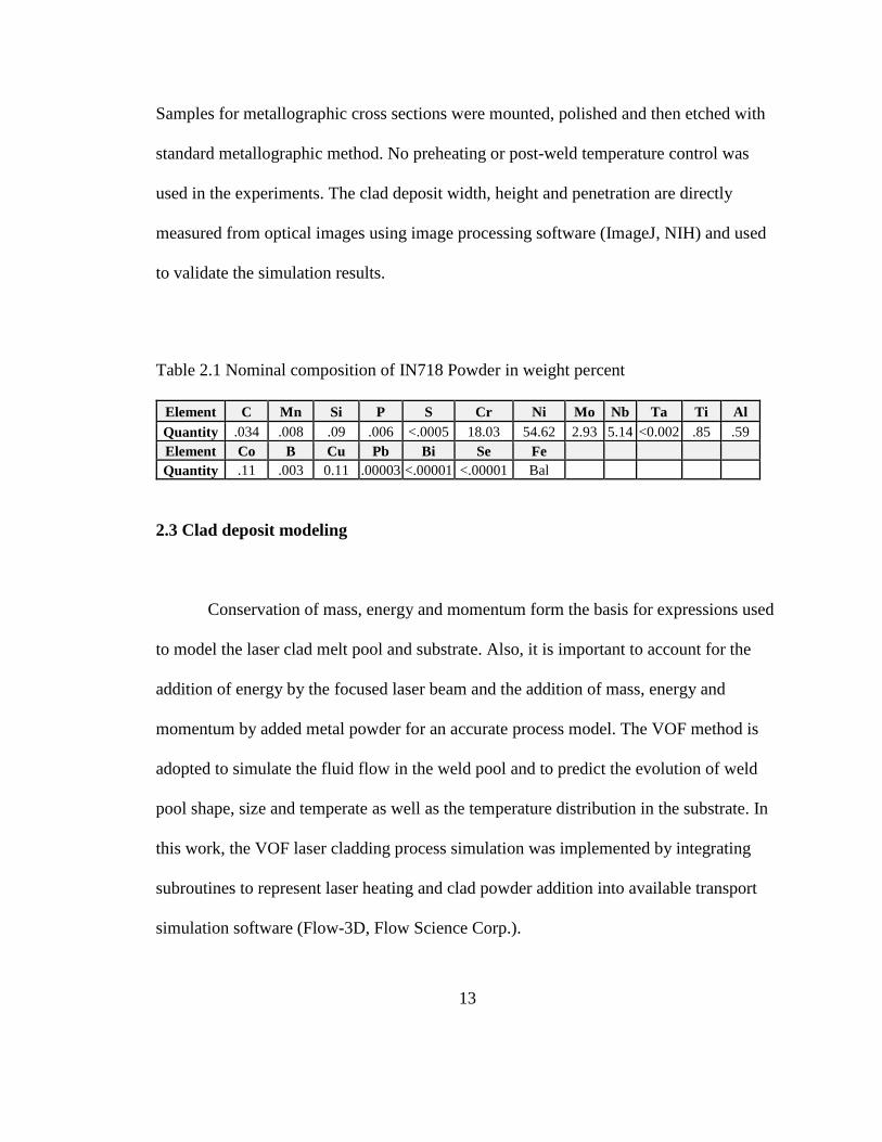
1.0mm and 1.016cm/s, respectively. Nominal composition of IN718 powder is shown in
Table 2.1. Metal powder screened with 100-325 mesh was used to build the clad deposit.
13
Samples for metallographic cross sections were mounted, polished and then etched with
standard metallographic method. No preheating or post-weld temperature control was
used in the experiments. The clad deposit width, height and penetration are directly
measured from optical images using image processing software (ImageJ, NIH) and used
to validate the simulation results.
Table 2.1 Nominal composition of IN718 Powder in weight percent
Element C Mn Si P S Cr Ni Mo Nb Ta Ti Al
Quantity .034 .008 .09 .006 <.0005 18.03 54.62 2.93 5.14 <0.002 .85 .59
Element Co B Cu Pb Bi Se Fe
Quantity .11 .003 0.11 .00003 <.00001 <.00001 Bal
2.3 Clad deposit modeling
Conservation of mass, energy and momentum form the basis for expressions used
to model the laser clad melt pool and substrate. Also, it is important to account for the
addition of energy by the focused laser beam and the addition of mass, energy and
momentum by added metal powder for an accurate process model. The VOF method is
adopted to simulate the fluid flow in the weld pool and to predict the evolution of weld
pool shape, size and temperate as well as the temperature distribution in the substrate. In
this work, the VOF laser cladding process simulation was implemented by integrating
subroutines to represent laser heating and clad powder addition into available transport
simulation software (Flow-3D, Flow Science Corp.).

14
2.3.1 Governing equations
Three dimensional mass conservation for VOF simulation of incompressible fluid
flow is expressed by the equation
smv
t
)(
(1)
where ρ is density of fluid in a numerical simulation mesh cell, t is time, v is liquid
metal velocity and sm is volumetric mass source rate. This conservation of mass relation
can be rewritten in terms of a scalar value F which explicitly refers to the mesh used to
discretize the simulation domain. F denotes volume fraction of fluid in a mesh cell
defined in the numerical simulation. By definition, the value of F = 0 indicates that the
corresponding simulation cell lies entirely within a void region and thus contains no fluid
while F = 1 indicates the cell is entirely occupied by fluid. Hence, any cell having F
values between 0 and 1 lies on the surface between fluid and void regions. The volume
fraction of fluid and volume fraction source rate can be defined in terms of the density of
fluid occupying a given cell as Equations (2, 3)
F0 (2)
Fms 0 (3)

15
where it is re-iterated that ρ refers to density of fluid in a cell (ratio of mass of fluid in
the cell and cell volume), ρ0 is density of the fluid and F is volume fraction of fluid in the
cell. A relation for conservation of F can be derived from Equations (1), (2) and (3), as
[12]
FFvt
F
)( (4)
By simultaneously solving the time-varying volume fraction conservation law along with
the momentum and energy conservation relations presented below, the time-varying
location and shape of the fluid-void boundary can be predicted.
For conservation of momentum, the fluid is assumed to be Newtonian with
laminar flow [13] The resulting conservation equation is
𝐷��
𝐷𝑡= −
1
𝜌𝛻𝑃 + 𝜇𝛻2𝑣 + 𝑔 [1 − 𝛽(𝑇 − 𝑇𝑚)] +
𝑝 𝑠
𝜌 (5)
where P is hydrodynamic pressure, μ is viscosity, g is gravitational acceleration, Tm is
melting temperature, β is thermal expansion constant, and 𝑝 𝑠 is a source term
representing the momentum addition rate corresponding to the captured filler material
droplets. Melt pool convection induced by buoyancy force due to thermal expansion of
the melt is typically negligible in comparison to flow induced by surface tension gradient
and was not included in this simulation.

16
In the simulations associated with free-surface fluid dynamics, the heat input, in
this case from the laser beam, is imposed as part of a surface heat flux boundary
condition. The heat is convected and conducted through clad the deposit melt pool and
substrate. Conservation of thermal energy used in the simulation is given as
𝜕ℎ
𝜕𝑡+(𝑣 ∙ 𝛻)ℎ=
1
𝜌(𝛻 ∙ λ𝛻𝑇) +
ℎ��
𝜌 (6)
where h is enthalpy, λ is thermal conductivity and ℎ�� is a source term representing
enthalpy addition rate associated with captured filler material droplets. The expression
above only considers thermal energy conservation in the weld pool. This is reasonable
since weld pools are relatively small and fluid flow speeds are moderate so the kinetic
and potential energy of the fluid is much smaller than the thermal energy. The latent heat
due to solid to liquid phase change is included in the enthalpy-temperature relationship.
2.3.2 Boundary conditions and physical properties for the simulation
The boundary conditions applied to the lateral edges of the substrate (illustrated in
Figure 2.2) were assumed as all solid walls to depict a rigid substrate with convection
heat loss coefficient 105 erg/cm2/C. The top and bottom surface boundary conditions
were defined as continuous to model semi-infinite domain in the surfaces. Laminar flow
and incompressible liquid were assumed for fluid flow in the weld pool. The simulation
was modeled in three dimensional Cartesian system for description of the transport
phenomena. The computation domain has dimensions of 0.8 cm in length (x-direction),
17
0.226 cm in width (y-direction) and 0.4 cm in height (z-direction) for transient flow
shown in Figure 2.2. The z-direction has 0.3 cm of substrate and 0.1 cm void region
above the substrate. The domain was meshed with cubic cells with 100 μm mesh size. To
model laser heating and powder mass, energy and momentum inputs, a moving source of
laser energy and mass flux is incorporated into the computation domain just above the top
surface of substrate (labeled “Coaxial Nozzle” in Figure 2.2(b)). The initial temperature
of the powder particles was assumed to be liquidus temperature. Thus, liquid particles
having 50 μm in diameter leave the nozzle exit and are injected into the liquid pool. Mesh
size and computation domain size independence of model results was verified. The
ambient temperature assumed for material and surroundings was 300 K. The material
used for both cladding powder and substrate was Ni-based superalloy, IN718.
Thermophysical properties and the various welding parameters applied to this simulation
were presented in Table 2.2 [14-16]. Fiber laser having flat-top distribution is used for
this simulation. The laser beam power, beam spot size, powder particle size and beam
travel speed were the values given directly from cladding process.

18
Figure 2.2 Boundary conditions for the edges of substrate and powder nozzle and (a) and
description of computation domain (b)
Table 2.2 Thermophysical properties of IN718 and process parameters used in numerical
model
Property Symbol Value Ref.
Specific Heat of Liquid CL 7.25e+06 (cm²/s²/K) 14
Specific Heat of Solid CS 5.77e+06 (cm²/s²/K) 14
Conductivity of Liquid λL 2.928e+06 (g-cm/s³/K) 14
Conductivity of Solid λS 2.792e+06 (g-cm/s³/K) 14
Latent Heat H 2.27e+09 (cm²/s²) 15
Power of Laser Beam P 350, 450, 550 (W) -
Beam Spot Size BS 1.0 (mm) -
Powder Feed Rate - 1.2 (g/min) -
Powder Particle Size - 50 (µm) -
Liquidus TL 1623 (K) 16
Solidus TS 1423 (K) 16
Travel speed of Laser
Beam V 1.016 (cm/s) -
Viscosity η 0.196*exp(5848/T) (mPa) 14
Density of Liquid DL 7.3 (g/cm3) 14
Density of Solid DS 8.19 (g/cm3) 14

19
2.4 Laser Cladding Process Mechanisms and Models
Laser cladding is a fusion welding process that uses a focused, moderate power-
density laser beam heat source and metal powder feed to melt and build-up layers of filler
material onto a substrate. Modeling of energy conservation in laser cladding needs to
account for losses that occur as the laser beam heats the substrate and the powder
particles during their flight from the nozzle exit to the substrate as well as the efficiency
of capture of laser powder into the deposited clad layer [17]. It is important to note that,
although laser beam-powder interaction attenuates the laser beam power that is incident
on the substrate, not all of the attenuated power is lost since some of it preheats the
powder. Most of this portion of this laser power is returned to the cladding process when
the heated particles are incorporated into the final clad deposit. Modeling of the laser
cladding process should thus take into account absorptance of laser energy by the
substrate and by powder particles, substrate and powder melting, transport phenomena in
the melt pool, efficiency of capture of powder particles in the clad deposit, and
solidification of melt to form a clad the deposit. Each of these topics is discussed in more
detail below.

20
2.4.1 Absorptance of laser beam energy
Absorptance of laser energy by the clad material is a key laser cladding process
parameter that varies with material composition and temperature. It has been found in
previous studies that a reasonable estimate of laser energy absorptance is provided by the
Hagen-Rubens [18] relationship. There, absorptance A(T) of the near infrared laser
energy is calculated from the temperature-varying electrical resistivity of the substrate
material ρe(T) by the relation
2/10 )](8[)( TTA e (7)
where ω is the angular frequency of the laser radiation (1.75 Х 1015 rad/s for fiber laser
radiation with wavelength λ = 1.07 Х 10-6 m) and ԑ0 is the permittivity of free space (8.85
Х 10-12 F/m). The equation can be rewritten in terms of electrical resistivity as
2/1)]([45.354)( TTA efl (8)
Expressions for temperature-varying resistivity [15] for solid and liquid IN718 are
31026 10713.910919.3005.0960.0)( TTTTe
for solid phase (9)
TTe
410364.1251.1)( for liquid phase (10)

21
The calculated optical absorptance at the solidus temperature is 35.6% which corresponds
well to a reported measurement of IN718 absorptance of 36% at Ts [19].
2.4.2 Energy balance
In this section, the relations used to calculate the distribution and losses of laser
beam power in the laser cladding process are discussed.
2.4.2.1. Power balance
The efficiency of use of laser beam power to form a molten clad deposit on a
substrate is decreased by power losses due to reflection, radiation, conduction and
convection from both the clad powder and substrate. With reference to the substrate, the
power balance can be expressed as [17]
.. ConvRadirpprsla QQQQQQQ (11)
where Qa is power absorbed by the substrate, Ql is total power in the laser beam, Qrs is
incident laser power reflected by the substrate, Qp is power absorbed by the fraction of
the powder stream that is not included in the clad deposit, Qrp is power reflected from the
powder stream, QRadi. is power lost from the substrate by radiation, and QConv. is power
lost from the substrate by convection. A visual representation of Equation (11) is shown

22
in Figure 2.3. It illustrates how the total laser power is redistributed by powder absorption
and the various losses.
Figure 2.3 Energy balance during laser cladding process
Experiment measurements of the power losses noted above have been reported by Gedda
[17] as 9% for Qrp + Qp , 1% for QRadi. + QConv. and 52% for Qrs. From the values, the
fraction of laser power absorbed by the substrate is calculated from Equation (11) as Qa =
38%. Notice that the reflection from substrate and powder stream are the largest losses
from the cladding process. Laser power absorption by an ionized plasma is neglected
because the near infrared laser wavelength (λ = 1.07 µm) and moderate focused power
density (7x10⁴ W/cm2) yield negligible absorption [20]. Figure 2.4 gives schematic flow
of energy losses.

23
Figure 2.4 Distribution of laser energy in the laser cladding process
Total absorbed energy by the substrate, Qa can be rewritten as
Fca QQQ (12)
where Qc is the fraction of the total laser power utilized in melting the clad deposit and
QF is the fraction of total laser power used in heating the substrate. Qc can be calculated
by
)( HTCAQ pc (13)
where A is area of weld bead, ν is laser beam travel speed, ρ is density of the melted
material, Cp is specific heat of the melted material, ΔT is temperature difference between
liquidus and room temperature and ΔH is latent heat of the clad melt. From the
calculation, it is shown that percentages of total laser power used for melting clad deposit
and heating of the substrate are Qc = 8.4% and QF = 29.6% respectively.

24
2.4.2.2. Powder catchment efficiency (η)
The powder catchment efficiency can be estimated by the fraction of powder
particles that impinge on the molten area of the substrate. For single-pass, single-layer
laser cladding, it may be assumed that any particles which strike the melt pool will
become part of the clad layer. In this approximation, all particles which do not impinge
on the pool can be considered as lost. This is reasonable because powder particles which
are not melted during their flight through the laser beam are likely to be reflected from
the solid substrate and those that are melted may adhere to the substrate but can still be
considered as lost because they do not contribute to formation of the single-pass clad
layer. With this assumption and an additional requirement that the powder jet
impingement area is larger than the melt pool, powder catchment efficiency can be
defined as ratio between the molten pool area and the substrate area impinged by the
power jet [21].
jet
liqjet
S
S (14)
Please note that assumptions the molten area can vary with laser power change and jet
area is larger than the molten pool area in this computation which are depicted in Figure
2.5. Jet area is constant for different laser powers while the molten pool area increases
proportionally as a function of the laser power.

25
Figure 2.5 Assumption for powder catchment efficiency
2.4.3 Melt pool fluid surface tension
The variation of surface temperature across the laser melt pool surface caused
fluid surface tension gradients and induced surface fluid flow from low to high surface
tension regions. Such Marangoni flows have been found to have significant effects on
weld pool circulation patterns and weld pool shape [22]. The amount of surface active
element sulfur in the alloy strongly affects the sign and magnitude of surface tension
gradients and associated Marangoni flow. It has been reported that the behavior of sulfur
in IN718 can be assumed to be the same as that in Fe-Ni-Cr alloys [9]. Thus, in this
study, the behavior of sulfur is accounted for by an equation applicable to a Fe-Ni-Cr-S
alloy [21]. Also, the effect of Cr-S interaction is considered in an activity term since Cr
changes the activity of S whereas Ni has negligible effects on the activity of S. The
values of surface tension gradient used in the simulation were calculated using Equation
(15) and material properties [14,23-25].

26
]exp1ln[)()(
0 RT
H
is
o
m
o
kaRTTTA
(15)
Here γ0m =1842 dyne/cm is the surface tension of the pure metal at reference melting
temperature T0, A=0.11 is a coefficient for the variation of surface tension at temperature
T above the liquidus, R= 8.314 J/mol-K is the gas constant, Γs = 2.27×10⁻⁹ g-mol/cm2 is
surface excess at saturation, k= 3.18×10⁻³ is entropy segregation constant and ΔH0= -
1.661× 10⁻⁵ J/mol is enthalpy of segregation. ai is the activity of species i in solution. For
the alloy used in the present study, transition temperature of surface tension gradient is
predicted at 1801K, marked as Ti in Figure 2.6.
Figure 2.6 The temperature and surface active element dependent values of surface
tension

27
2.4.4 Melt solidification
In metal alloys, it is known that solidification morphology is significantly affected
by the combination of temperature gradient (G) in the liquid at the solidification
boundary and solidification rate (R) as presented in Figure 2.7 [26].
Figure 2.7 Effect of G and R on solidification morphology
A planar growth mode occurs when G is very high or/and R is extremely low
value. As R increases, the solidification morphology can shift to cellular, columnar and
then equiaxed dendritic. Most metal alloys solidify in cellular or columnar dendritic
mode. The cellular and columnar growth modes are produced when the growth of crystal
structures occurs without formation of any secondary dendrite arms. If additional dendrite
arms form, the solidification mode shifts to dendritic. Equiaxed dendritic morphology is
possible only when G is very low.

28
As the cooling rate, which is the product of G and R, increases, finer
microstructures are produced. Note that high cooling rate results in much closer spacing
between cellular or dendrite arms. Eventually, the finer microstructure leads to increased
mechanical properties. In general, it is known that cooling rate in laser cladding varies
with the processing parameters [2] and is faster (102 -106 K/s) than that of conventional
casting. Therefore, the influence of processing parameters on G and R and the
solidification morphologies that occur will be assessed in this study.
2.5 Results and discussion
2.5.1 Powder catchment efficiency
The metal powder catchment efficiency [27] and resulting mass flow rate of
powder into the melt pool used in the simulation were calculated from experimental
results and results given in the literature. As shown in Table 2.3, the catchment efficiency
was 45% and the mass flow rate was 1.2 g/min for a laser 550W. The mass flow rates at
350W and 450W were proportionally adjusted from the 550W value based on the laser
power ratio. Lower laser power creates smaller molten area on the substrate, Sliqjet
according to Equation (14). By scaling, the molten pool area at 350W is 63.6% of the
area at 550W. From the assumptions, the efficiencies for 350W and 450W are calculated
to be 28.62% and 36.81%, respectively.

29
Table 2.3 Calculation of catchment efficiency
Power Mass Flow Rate Setting
(g/sec)
Efficiency
(%)
Mass Rate into Molten Pool
(g/sec)
350W
0.020
28.62% 0.00573
450W 36.81% 0.00736
550W 45.00% 0.00900
2.5.2 Melt pool size: experiment vs. simulation
The width, height and penetration depth of the deposit are compared to the
simulation results by X-Y (a) and Y-Z (b) views in Figures 2.8(a) and (b). A dotted line
indicating the simulation liquid-solid weld pool boundary is overlaid onto each
corresponding experimental image. These results show that simulated weld pool shapes
and dimensions are comparable to the experiments. Quantitative comparisons of
simulated and experimental clad width, height and penetration depth are shown in Figure
2.9. The weld pool dimensional are plotted for laser powers of 350W, 450W and 550W.
The experimental results are comparable to the simulation predictions. Note that
increased laser power leads to increased weld width and penetration depth while the clad
height is relatively constant. The clad height is relatively constant because the powder
flux within the jet area is constant and the jet area is larger than the weld pool surface
area in all simulation cases (c.f. Figure 2.5). Thus, the larger melt pool surface area
results in increased powder catchment efficiency and more mass addition to the molten
pool (c.f. Table 2.3) but not increased clad height.

30
Figure 2.8 Top-down (a) and cross section (b) views at the same magnification for
comparison of simulated and experimental single pass laser clad melt pool and deposits at
various powers. Dashed lines in simulation images show the position of liquidus isotherm
while dashed lines in experimental images show the liquidus isotherm from the
corresponding simulation
Figure 2.9 Comparison of simulated and experimental weld pool dimensions

31
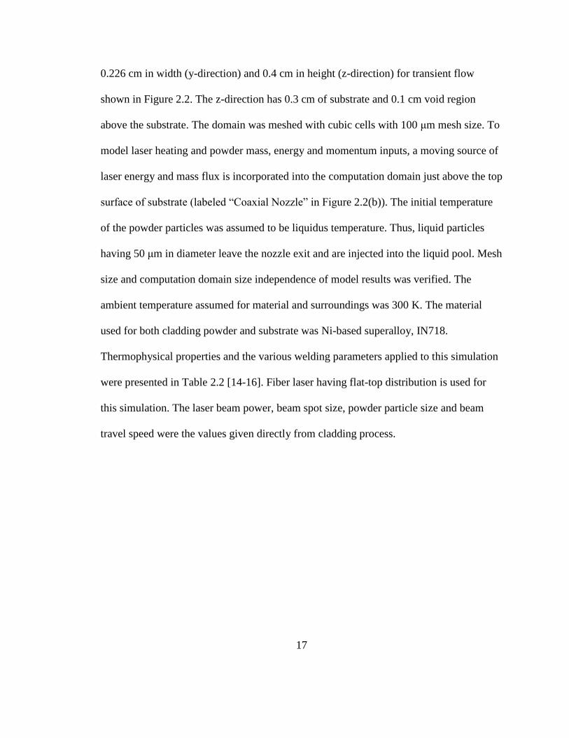
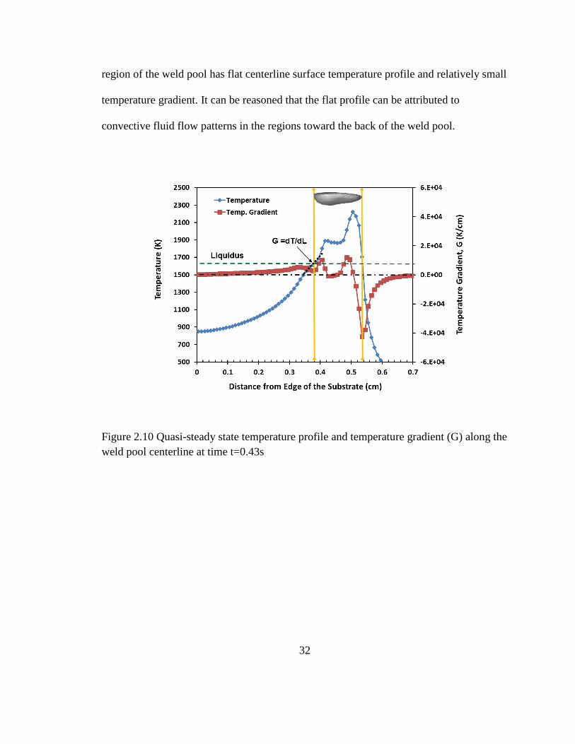
2.5.3 Fluid flow patterns in melt pool
As discussed in section 2.4.3, a fluid circulation known as Marangoni flow occurs
the weld pool surface. Resulting convective flow in the melt produces weld pool
temperature gradients. Figure 2.10 shows the temperature profile and corresponding
temperature gradient, G along the clad centerline t = 0.43 sec. The quasi-steady state
solidification rate on the weld centerline at the back of the weld pool is constant and
equal to the laser travel speed, 1.016cm/s. The calculated values of G = 3.0*103 K/cm and
R = 1.016 cm/s are comparable to values found in literature [28] for the observed
columnar dendritic solidification mode. Although other conditions in the above cited
reference vary somewhat from those applicable for laser cladding, it is reasonable to
expect similar solidification morphology. The simulated weld pool shape is shown in a
grey inset to explain the relationships between temperature profiles, temperature gradient,
fluid flow pattern and weld pool shape. The orange line indicates the weld pool length,
which ranges from 0.380 cm to 0.537 cm at the simulation time 0.43 sec. Surface
temperature on the weld centerline increases from liquidus at the back of the pool to
about 1900 K and the remains constant over a region that also corresponds to the deepest
weld pool penetration. Further towards the front of the pool, the surface is heated by laser
beam heat input, the temperature increases further. The variation of weld pool centerline
surface temperature gradient is calculated as the first derivative of surface temperature.
The temperature gradient equals zero near the center of the laser focus spot (around 0.5
cm) and becomes negative at the front edge of the pool. Note that the deep-penetration
32
region of the weld pool has flat centerline surface temperature profile and relatively small
temperature gradient. It can be reasoned that the flat profile can be attributed to
convective fluid flow patterns in the regions toward the back of the weld pool.
Figure 2.10 Quasi-steady state temperature profile and temperature gradient (G) along the
weld pool centerline at time t=0.43s

33
Figure 2.11 Longitudinal-section view showing fluid flow and mixing in the laser clad
melt pool, the location of laser focus spot. The green dot indicates the location of the
weld pool surface with temperature Ti where surface tension gradient transitions from
positive to negative.
Figure 2.11 displays the flow pattern in the weld pool. Surface areas with positive
and negative surface tension gradient are both found on this weld pool. The transition
temperature Ti that divides the two regions is calculated from Equation (15) and
displayed in the plot in Figure 2.6. Its location on the pool surface is represented with
green dot in Figure 2.11. Surface tension gradients generate surface flow from areas with
low surface tension to areas with high surface tension. Thus, surface flow tends to carry
higher temperature fluid from the area heated by the laser beam towards the trailing edge.
However, at a same time, flows originating at the cooler back edge of the pool tend to
deliver lower temperature fluid towards the front. The two opposing surface flows end up

34
colliding and mixing in a region intermediate between the laser focus spot and the trailing
pool edge where the liquid surface temperature is equal to the transition temperature Ti
(represented by the green dot in Figure 2.11). As a result of the mixing of opposing
hotter and cooler flows from the front and rear portions of the melt pool, temperature is
relatively uniform in that region and gradient is correspondingly small (c.f. Figure 2.10).
Also the downward flow (produced by colliding surface flows) is strongest and the
resulting weld pool penetration is deepest near this point. Although experimental
validation of this weld pool penetration contour has not been completed, the fact that
simulation predictions of clad penetration, width and height are close to experimental
values provides indirect evidence that the weld pool contour is reasonable. We also note
that a similar pool profile has been predicted in autogenous gas tungsten arc welding
[29].
The weld pool surface tension and fluid flow patterns are shown in 2D and 3D
plots in Figure 2.12. It is seen that two opposing flows meet at the line showing the
position of the transition temperature Ti (b) and generate downward mixing flow along
this line (c). In Figure 2.13, the variation of fluid flow patterns are assessed in
consecutive 2D cross-sections spaced evenly along the X-axis.

35
Figure 2.12 Three dimensional depiction of weld pool convection flows (c) with inset
figures showing temperature-dependent surface tension (a) and surface temperature (b).
In (a), surface tension gradient switches from positive to negative at Ti. In (b), Ti
separates the positive (blue) and negative (red) surface tension regions. The two opposing
surface flows impinge along the line where surface temperature equals Ti.

36
Figure 2.13 3D and 2D plots showing fluid flow and mixing in laser clad melt pool
Dominant outward-directed Y-axis Marangoni flows are observed on the weld
surface with maximum velocity 26.5 cm/s in section 1. This pattern of the flow indicates
that only negative surface tension gradient resulting in completely outward flow is
present at this region. In section 2, the main Marangoni flow is still outward direction at
the center of the weld pool due to negative surface tension gradient and relatively high
temperature at that region. Note that inward fluid flows which are opposite to the flow at
the center in direction are observed near the outermost edges of the pool. This flow
pattern indicates switching of surface tension gradient from negative to positive. The

37
fluid velocity is reduced to 21.8cm/s due to the opposing flow. In section 3, prominent
inward and outward surface flows with comparable velocities exist. Downward flow is
found at the intermediate region between the weld edge and center where the surface
flows collide. As the distance from laser beam increases, weld pool temperature
decreases and eventually it reaches the temperature switching surface tension gradient.
Hence, the region showing the dominant positive gradient keeps widening but the
expansion stops at the gradient transition region. The maximum flow velocity is found at
the region where the two opposite flows meet. In section 4, the gradient is fully switched
to positive. Thus, only inward and downward flows are seen.
2.6 Summary, conclusions and future work
A transport simulation of the laser cladding process was used to understand the
effect of convection flow on the cladding melt pool formation and solidification
conditions in IN718 deposits. Predicted clad width, height and penetration depth at
different laser powers were found to be comparable to experimental measurements. Due
to heat flow in the melt pool induced by Marangoni convection, the most deeply
penetrated region was formed towards the back of the weld pool, behind the laser focus
spot but ahead of the rear solidification boundary. The increased penetration was formed
in this region by impingement of opposing surface flows caused by positive and negative
X-axis surface tension gradients along the weld centerline. The flow pattern also caused
the weld pool to have a relatively flat rear boundary and contributed to a relatively

38
uniform temperature distribution in the melt pool in the region where opposing surface
flows impinged. Also, temperature gradient was calculated along the weld pool center
line and, in combination with the centerline solidification rate at the back edge of the
weld pool was used to predict columnar dendritic solidification. The correspondence with
the observed weld pool solidification mode was noted. Future simulation and
experimental efforts are planned to extend the work to multiple layer clads and to
experimentally validate the weld pool convection patterns and penetration profiles
predicted by the simulations.
2.7 Acknowledgement
The authors would like to thank Rolls-Royce Corporation for the funding support and
providing laser cladding samples in this work. They also appreciate NSF-I/UCRC: Center
for Integrative Materials Joining Science for Energy Applications. The authors express
their thanks to J.S.Bader for helpful suggestions and interest in this project.

39
2.8 References
1. Zhong M, Liu W (2010) Laser surface cladding: The state of the art and challenges.
Journal of Mechanical Engineering Science 224(C5):1041-1060.
2. A.Weisheit, Gasser A, Backes G, Jambor T, Pirch N, Wissenbach K (2013) Laser-
assisted fabrication of materials - direct laser cladding , current status and future scope of
application, vol 161. Springer New York
3. Hoadley AFA, Rappaz M (1992) A thermal model of laser cladding by powder
injection. Metallurgical Transactions B 23(5):631-642.
4. Picasso M, Rappaz M (1994) Laser-powder-material interactions in the laser cladding
process Journal De Physique IV 4(C4):27-33.
5. Toyserkani E, Khajepour A, Corbin S (2004) 3-d finite element modeling of laser
cladding by powder injection: Effects of laser pulse shaping on the process. Optics and
lasers in engineering 41(6):849-867.
6. Choi J, Han L, Hua Y (2005) Modeling and experiments of laser cladding with droplet
injection. Journal of Heat Transfer 127(9):978-986.
7. Wen S, Shin YC (2010) Modeling of transport phenomena during the coaxial laser
direct deposition process. Journal of Applied Physics 108(4):044908
8. Sahoo P, Debroy T, Mcnallan MJ (1988) Surface tension of binary metal-surface
active solute systems under conditions relevant to welding metallurgy. Metallurgical
Transactions B 19B(3):483-491.
9. Lee PD, Quested PN, McLean M (1998) Modelling of marangoni effects in electron
beam melting. Philosophical Transactions of the Royal Society of London
356(1739):1027-1043.
10. Su Y, Mills KC (2005) A model to calculate surface tension of commercial alloys.
Journal of Materials Science 40(9-10):2185-2190.
11. Zhao CX, Kwakernaak C, Pan Y, Richardson IM, Saldi Z, Kenjeres S, Kleijn CR
(2010) The effect of oxygen on transitional marangoni flow in laser spot welding. Acta
Materialia 58(19):6345-6357.

40
12. Cho MH, Lim YC, Farson DF (2006) Simulation of weld pool dynamics in the
stationary pulsed gas metal arc welding process and final weld shape. Welding Journal
85(12):271-s to 283-s.
13. Cho JH, Farson DF, Milewski JO, Hollis KJ (2009) Weld pool flows during initial
stages of keyhole formation in laser welding. Journal of Physics D: Applied Physics
42(17):175502.
14. Mills KC (2002) Recommended values of thermophysical properties for selected
commercial alloys. Woodhead, Cambridge, England
15. Pottlacher G, Hosaeus H, Kaschnitz E, Seifter A (2002) Thermophysical properties of
solid and liquid inconel 718 alloy. Scandinavian Journal of Metallurgy 31(3):161-168.
16. Lewandowski MS, Overfelt RA (1999) High temperature deformation behavior of
solid and semi-solid alloy 718. Acta Materialia 47(18):4695-4710.
17. Gedda H, Powell J, Wahlstrom G, Li WB, Engstrom H, Magnusson C (2002) Energy
redistribution during co2 laser cladding. Journal of Laser Applications 14(2):78-82.
18. Xie J, Kart A, Rothenflue JA, Latham WP (1997) Temperature-dependent
absorptivity and cutting capability of CO2 , Nd:YAG and chemical oxygen-iodine lasers.
Journal of Laser Applications 9 (2):77-85.
19. Shelton JA, Shin YC (2010) Comparative evaluation of laser-assisted micro-milling
for aisi 316, aisi 422, Ti-6Al-4V and inconel 718 in a side-cutting configuration. Journal
of Micromechanics and Microengineering 20(7):075012.
20. Kim KR, Farson DF (2001) Co2 laser-plume interaction in materials processing.
Journal of Applied Physics 89(1):681-688.
21. Picasso M, Marsden CF, Wagniere JD, Frenk A, Rappaz M (1994) A simple but
realistic model for laser cladding. Metallurgical and Materials Transactions B
25B(2):281-291.
22. Kou S (2012) Fluid flow and solidification in welding: Three decades of fundamental
research at the university of wisconsin. Welding Journal 91(11):287S-302S.

41
23. Zacharia T, David SA, Vitek JM, Debroy T (1989) Weld pool development during
gta and laser beam welding of type 304 stainless steel--part I: Theoretical analysis.
Welding Journal 68(12):499-s to 509-s.
24. Mcnallan MJ, Debroy T (1991) Effect of temperature and composition on surface
tension in fe-ni-cr alloys containing sulfur. Metallurgical Transactions B 22B(4):557-560.
25. Anderson TD, DuPont JN, DebRoy T (2010) Origin of stray grain formation in
single-crystal superalloy weld pools from heat transfer and fluid flow modeling. Acta
Materialia 58(4):1441-1454.
26. Kou S (2003) Welding metallurgy. 2nd edn. John Wiley & Sons, New Jersey
27. Weisheit A, Backes G, Stromeyer R, Gasser A, Wissenbach K, Poprawe R Powder
injection: The key to reconditioning and generating components using laser cladding. In
Proceedings of International Congress on Advanced Materials and Processes, Materials
Week 2001, Munich, Germany. pp pp. 1-7
28. Lim YC, Yu X, Cho JH, Sosa J, Farson DF, Babu SS, McCracken S, Flesner B
(2010) Effect of magnetic stirring on grain structure refinement--part i: Autogenous
nickel alloy welds. Science and Technology of Welding and Joining 15(7):583-589.
29. Zhao YZ, Lei YP, Shi YW (2005) Effects of surface-active elements sulfur on flow
patterns of welding pool. Journal of Materials Science & Technology 21(03):408-414.

42
Chapter 3: Effect of Fluid Convection on Dendrite Arm Spacing in
Laser Deposition
3.1 Introduction
Methods for increasing the overall efficiency of aircraft engines and gas turbines
can reduce operating cost and environmental impact (e.g. emission of CO2) and has long
been an issue among manufactures of these systems. Higher operating temperature is
effective to increases the efficiency of turbines but components are exposed to higher
temperatures and their properties may be significantly degraded. For example, in high-
efficiency gas turbine engines [1], the gas stream passing through combustor has a
temperature as high as 1500 °C. Turbine blades are exposed to high temperatures, a
corrosive gas atmosphere and high operating stresses. Wear is particularly severe at the
tips of the blades since high operating efficiency requires small clearance between
rotating turbine blade tips and the outer stator casing. This small clearance contributes to
tip wear by mechanisms of erosion, corrosion, oxidation, deformation and adhesive
transfer, singly or in combination [2]. Since tip wear limits the life of blade life, repairing
worn turbine blade tips is of great economic interest [3].

43
Laser cladding technology has been popularly utilized to apply worn protection
layer on metallic surfaces or to repair damaged surfaces of structural parts [4]. In laser
cladding with blown powder, the powdered metal clad materials are delivered through
multiple powder feed nozzles placed annularly around the laser beam, into a laser-
generated melt pool as a form of powder particles that are carried by an inert gas [5]. The
schematic description is shown in Figure 2.1 [6]. Some powder particles are heated by the
laser beam during flight and others are melted once they alight on the liquid melt pool
surface. Only powder particles landing in melt pool contribute to formation of the clad
deposit layer after solidification. The other particles alighting outside of melt pool will
ricochet off and be lost. The development of laser cladding process is required for
generally-applicable accurate model. However, the complexity associated with
interaction between powder particles, laser beam and substrate makes simulation
difficult. Total absorbed laser power density is modified by interaction between laser
beam and powder cloud. Moreover, powder input accompanies with corresponding
amount of mass and momentum into the melt pool. Thus, temperature distribution and
fluid flow patterns in the weld pool will be changed and subsequently resultant shape of
the clad deposit.
Ni superalloy is the metal most widely used for hot section component in the
engine because it is very resistant to corrosion and maintains reasonably high strength at
elevated temperature. In aircraft engine and gas turbine engine systems, single crystalline
structures have been popularly used due to better creep resistance and fatigue behavior.
However, the production cost of single crystal is not only significantly expensive due to

44
complexity of process parameter control but also Ni superalloy itself is high in price [7].
Thus, repair of the damaged parts instead of replacing have been strongly required from
industry fields. In this research, laser cladding process is used to repair the damaged part.
However, property degradation and micro-cracks are observed in the Ni superalloy clad
deposit. Therefore, a better understanding for the parameter-microstructure relationship
of the clad deposit is required to solve the problems.
3.1.1 Fluid Dynamics and its effect on weld pool shape
The variation of surface tension that is present on the laser melt pool causes the
molten metal to flow from low surface tension to higher surface tension region. The
variation in the surface tension is mostly derived from two sources. Surface tension is a
temperature dependent value so that temperature gradient across the weld pool results in
surface tension gradient on the melt pool surface. In addition, for the alloys, the
compositional gradient on the weld pool surface leads to surface tension gradients, and
changes fluid flow patterns.
Such Marangoni flows have been found by Heiple et al. [8,9] and its significance
on weld pool circulation patterns and weld pool shape was confirmed by other
researchers [10,11]. It is well known that the fluid always moves from low to higher
surface tension region [12,13]. In negative surface tension gradient for pure metal (a), the
surface tension induces radially outward flow from high (center, C) to lower temperature
region (edge, E) where the weld pool becomes shallow and wide whereas in positive
45
gradient region (b), the flow moves radially inwards from low (edge, E) to higher
temperature region (center, C) where the weld pool becomes deep and narrow. It is
pointed out that positive to negative transition at a certain temperature can occur and
produce complex fluid flow (c). Ti is the transition temperature of surface tension.
Figure 3.1 Different fluid flow pattern produced by different surface tension gradient
As seen previously, the compositional gradient in alloy alters Marangoni flow
patterns that change the shape of weld pool. Thus, many studies have been conducted
with regard to the compositional effects. The influence of composition and temperature
on surface tension in the Ni-S system has been previously investigated [14]. The effect of
sulfur and oxygen on surface tension and its gradient was reported for electron beam
melting of IN718 [15]. The developed calculation model was suggested to know the

46
effect of sulfur and oxygen at ppm level [16]. Detailed study of the influence of oxygen
and temperature gradient on surface tension was recently reported with stainless steels in
A-TIG welding and in laser spot welding [17,18]. However, the composition effect on
fluid pattern and associated laser melt pool shape has not been studied in prior laser
cladding simulations.
3.1.2 Correlation of the weld pool shape with solidification microstructure
During transformation from liquid to solid, the solidification behavior controls the
distribution of solute, and the size and morphology of grains [19]. The critical parameters
determining the solidification microstructure are the temperature gradient G,
solidification rate R, undercooling T, and alloy constitution. Depending on these
conditions, the microscopic shape of the solid-liquid interface varies from planar to
cellular dendritic, to columnar dendritic, and to equiaxed dendritic. Pure metals have a
planar solid-liquid interface and solidify as a single crystal. However, in alloys, the
factors affecting solidification morphology are more complicated because redistribution
of alloy elements leads to concentration gradients adjacent the solid-liquid interface.
When the actual temperature of liquid ahead of the solidification interface is lower than
the equilibrium liquidus temperature corresponding to the composition variation,
constitutional supercooling occurs and the planar interface is unstable. The criteria for the
stability of the planar solid-liquid interface can be expressed as [20]

47
GL
R>
∆𝑇𝑠
DL , (1)
where GL is the temperature gradient in liquid region, R is the solidification rate, Ts is
the solidus and liquidus temperature difference and DL is the diffusion coefficient in
liquid region. Therefore, the constitutional supercooling determines the solidification
mode at the rear solidification boundary of a traveling weld pool.
The size and morphology of the solidified microstructure can be revealed by using
the combined form of temperature gradient G and solidification growth rate R which is
shown in Figure 3.2 [20]. The ratio of G/R indicates solidification morphology whereas
the product of G and R represents the scale of the solidification microstructure.
Figure 3.2 The effect of G and R on the solidification morphology and size
48
A planar growth occurs when G is very high or/and R is extremely low value. As
R increases, the solidification morphology can shift to cellular, columnar and then
equiaxed dendritic. Most metal alloys are solidified in cellular or columnar dendritic
mode. The cellular and columnar growth mode are produced when the growth of crystal
structures occurs without formation of any secondary dendrite arms. If additional dendrite
arms form, the structures are shifted to dendritic mode. Equiaxed morphology is possible
only when G is very low.
As the cooling rate of the liquid in front of the solidification boundary (which is
the product of G and R) increases, a finer dendritic solidification microstructure results.
Eventually, the finer microstructure leads to increased mechanical property of metals. In
general, it’s known that cooling rate in laser cladding typically varies in the range from
102 -106 K/s, than that of conventional casting and it is a function of the processing
parameters [4].
As seen above, in addition to the temperature gradient G, the solidification rate R
plays a very important role in determining solidification size and morphology. However,
measuring precise G and R values is very difficult because they vary considerably from
point to point along the weld pool boundary. Furthermore, measuring GL is very
complicated due to fluid convection in the weld pool. Therefore, numerical simulation
including heat transfer and fluid convection is a good alternative to experimental
measurement of G and R [21].
Analytical models for the prediction of solidification morphology and size have
been presented in prior publications. Columnar to equiaxed transition (CET) was

49
predicted by a theoretical expression that included solidification variables G and R [22].
Additional studies have been carried out to understand the degradation of mechanical
properties caused by equiaxed grains in laser and electron beam welds on Ni-based single
crystal superalloys [23,24]. Relationships for the prediction of secondary dendrite arm
spacing (SDAS) from G and R values have been presented for hybrid laser-arc welding
[25]. Results showed that the size of the microstructure varied by location in the weld
pool.
The main purpose of this study is to use a numerical simulation to obtain thermal
conditions G, R and solidification cooling rate ,and then to use these values in theoretical
models for prediction of the primary dendrite arm spacing. Dependence of microstructure
in size on solidification variables is investigated by comparison of the predicted primary
dendrite arm spacing using G and R as an input to experimental measurements.
3.2 Flow and Solidification Model
3.2.1 Weld pool shape and solidification conditions
In order to obtain high quality cladding conditions experimentally, a large number
of experiments are needed because numerous variables such as laser power, speed,
powder feed rate and catchment efficiency must be optimized [26]. Moreover, direct
measurement of weld pool flow and temperature distribution is even more difficult since
the pool is very hot and small, and heating and cooling rates are very fast. An accurate

50
numerical simulation can provide the weld pool conditions without the difficulties
associated with measurements. In this work, a 3D weld pool simulation was implemented
and used to predict weld pool shape, temperature gradient G and solidification rate R for
single layer, single track deposits. Heat transfer, fluid flow, mass addition, and laser-
powder-substrate interaction were included in the simulation. Ni-based superalloy, IN718
was used for clad powder and substrate properties in the simulation.
During the laser cladding process, laser-heated powder is continuously added and
the mass, momentum and energy additions change the weld pool shape and clad
geometry. Thus, three important governing equations of mass, energy and momentum
conservation should be solved for reasonable modeling of laser cladding. To investigate
fluid behavior in the weld pool and free surface change, the volume of fluid (VOF)
method is utilized in this study. The conservation equations are solved by commercial
software (Flow-3D, Flow Science Corp.).
𝜕𝜌
𝜕𝑡+ 𝛻 ∙ (𝑣 𝜌) = ��𝑠 Conservation of mass, (2)
𝜕ℎ
𝜕𝑡+(𝑣 ∙ 𝛻)ℎ=
1
𝜌(𝛻 ∙ 𝜎𝛻𝑇) +
ℎ��
𝜌 Conservation of energy, (3)
𝐷��
𝐷𝑡= −
1
𝜌𝛻𝑃 + 𝜇𝛻2𝑣 + 𝑔 [1 − 𝛽(𝑇 − 𝑇𝑚)] +
𝑝 𝑠
𝜌 Conservation of momentum. (4)

51
Time-varying shape and location of fluid-void boundary can be obtained by
simultaneously solving the conservation equations. The fluid is assumed to be
incompressible and Newtonian with laminar flow. ρ is fluid density, t is time, v
is molten
metal velocity, ��𝑠 is source term representing the mass addition rate of filler metal
droplets that are captured in the molten pool, h is enthalpy, σ is thermal conductivity ℎ�� is
a source term representing enthalpy addition rate associated with captured filler material
droplets, P is hydrodynamic pressure, μ is viscosity, g is gravitational acceleration in z
direction, β is constant of thermal expansion, Tm is melting temperature, and 𝑝 𝑠 is a
source term representing the momentum addition rate corresponding to the captured filler
material droplets.
𝜕𝐹
𝜕𝑡+ 𝛻 ∙ (𝑣 𝐹) = 𝐹�� Conservation of fluid volume fraction, (5)
where F is volume fraction of fluid in a cell. Thus, the value of F only exists from F=0
(=void region) to F=1 (=entirely occupied region by fluid). �� denotes the change in F
associated with density of fluid and mass source rate.
For reasonably accurate description of the laser cladding process, several
calibrations are made in this study. More details of the calibrations and approaches for
the simulation were presented in a separate paper [6] so a brief summary is presented
here. An approximation of laser energy absorptance was given by Hagen-Rubens

52
relationship [27]. Absorptance is calculated from temperature-varying resistivity of the
substrate and clad material (assumed to have the same composition)
𝐴(𝑇) = [8𝜀0𝜔𝜌𝑒]1/2 Hagen-Rubens relationship, (6)
where A is absorptance, ε0 is permittivity of free space, ω is the angular frequency of
laser radiation (1.75 Х 1015 rad/s for fiber laser radiation with wavelength λ = 1.07 Х 10-6
m), and ρe is electrical resistivity of substrate.
For laser cladding, it may be assumed that any particles which do not strike the
molten pool can be considered to be lost. This is reasonable because powder particles
which impinge on solid substrate are likely to be reflected and thus not contribute to
formation of the clad deposit. Therefore, the powder catchment efficiency ϕ can be
defined as a ratio between the area of molten pool Sm and area of substrate which is
impinged by the powder jet, Sjet [26]
φ = 𝑆𝑚/𝑆𝐽𝑒𝑡. (7)
3.2.2 Temperature gradient and solidification rate
Temperature gradient vector G is normal to solid-liquid interface of the weld pool
and has components Gx, Gy and Gz. These components are obtained directly from the

53
simulated 3D weld pool by differentiating temperature profile at the liquid interfaces. The
laser beam travelling direction is parallel to the X-axis and substrate surface normal is
along the Z-axis. Once the components Gx, Gy and Gz are obtained, the temperature
gradient normal to the solidification front G can be calculated with the expression
|𝑮| = 𝐺 = √𝐺𝑥2 + 𝐺𝑦
2 + 𝐺𝑧2. (8)
It is known that the solidification rate on the liquid side of the solid-liquid
boundary strongly influences the scale of the weld microstructure [28]. For steady state
conditions, the magnitude of the solidification rate (R) at any point on the solid-liquid
interface is geometrically related to the laser scanning speed (Rb) and angle between the
solidification boundary and the welding travel direction at the point of interest [29]. The
solidification rate R can be calculated by
|𝑹| = 𝑅 = |𝑹𝑏| 𝑐𝑜𝑠 𝜃. (9)
In equation (9), ϴ is the angle between solid-liquid interface normal and beam
travel direction. In a Cartesian coordinate system, cosθ can be expressed by
𝐺𝑥/√𝐺𝑥2 + 𝐺𝑦
2 + 𝐺𝑧2 [30]. R is obtained at three different heights on the simulated weld
pool solidification boundary spaced at 100 µm (see Figures 3.4 and 3.5). Note that R is
zero (minimum) at the bottom and the outermost edge of the weld pool because the
boundary normal is at an angle ϴ = 90 degrees to the beam travel direction. R becomes
same as Rb (maximum) at the trailing edge of the upper surface of the weld pool because
its angle ϴ is zero degrees to the travel direction.

54
3.2.3 Solidification Microstructure Models
Several theoretical models have been proposed to describe the dependency of size
of microstructure on solidification conditions. The present work considered models
proposed by Kurz-Fisher [31] and Trivedi [32], in which primary dendrite arm spacing
(PDAS) of the dendritic solidification microstructure at various locations along the weld
pool solidification boundary is predicted from the corresponding magnitudes of steady-
state solidification temperature gradient G and solidification rate R. The Kurz-Fisher and
Trivedi models are presented in equations (10) and (11), respectively [33,34]
𝜆𝑃𝐷𝐴𝑆 = 4.3∆𝑇𝑛0.5 (
𝐷𝐿𝛤
𝛥𝑇0𝑘)0.25
𝐺−0.5𝑅−0.25 Kurz-Fisher, (10)
𝜆𝑃𝐷𝐴𝑆 = 2.83(𝐿𝛥𝑇0𝑘𝐷𝐿𝛤)0.25𝐺−0.5𝑅−0.25 Trivedi. (11)
Here Tn is the non-equilibrium solidification range for IN718, L is the constant
of harmonic perturbation, DL is the diffusion coefficient in liquid, Γ is Gibbs-Thomson
coefficient, T0 is the equilibrium solidification temperature range, and k is the partition
coefficient. The physical properties used in theoretical model are listed in Table 3.1.

55
Table 3.1 Physical properties of nickel based superalloy used in theoretical prediction
Property Symbol Value (units) Ref.
Non-equilibrium solidification range Tn 200 (K) 35
Constant of harmonic perturbation L 28 31
Diffusion coefficient in liquid DL 3.0*10-9 (m2/s) 36
Gibbs-Thomson coefficient Γ 1.0*10-7 (K⋅m) 36
Equilibrium solidification range T0 105 (K) 37
Partition coefficient k 0.48 36
3.3 Experimental
A single path, single layer clad track was formed by depositing IN718 powder on
an IN718 substrate. The substrate thickness was 0.226 cm, the laser power used to build
the clad layer was 550W, laser spot size was 1mm, the powder feed rate was 1.2 g/min
and the travel speed was 1.016 cm/s. The deposit was cross-sectioned, metallographically
prepared and photographed. PDAS was directly measured from an optical image taken
from the center of the deposit using image processing software (ImageJ, NIH).

56
Figure 3.3 Measured primary dendrite arm spacing from a single layer clad deposit
PDAS was measured from an image of a cross section of a single track, single
layer clad deposit as shown in Figure 3.3. The deposit width was 1.77 mm and deposit
height was 100 µm. The predicted PDAS within the measurement area varied from 8.1 to
11.5 µm with a mean value of about 10 µm.
3.4 Numerical Model Results and Solidification Microstructure Prediction
In Figure 3.4, the weld pool solidification rate R predicted by the numerical
model is plotted in X-Y-Z plane with a simulated weld pool shaded gray. The 3D weld
pool is analyzed at the three different height sections A, B and C separated by 100 µm.
The magnitude of solidification rate is illustrated by colored points (note that dark red is
the maximum and dark blue is minimum value). The maximum solidification rate R is
found on the weld centerline (Y=0) whereas the minimum value is at the outermost
lateral weld edge (Y=max. weld width). It is also observed that the solidification rate near
the weld pool top surface is higher than near the weld pool bottom. Note that the
--- Kurz and Fisher
— Trivedi
Weld
Edge

57
solidification rate at the weld center seems to be nearly constant even though the height
changes from level A to B. However, the solidification rate decreases significantly from
height B to C. In other words, the solidification rate maintains the travel speed of the
beam at heights A and B whereas it decreases at height C. This can be explained by the
fact that the angle θ is relatively small at both heights A and B at the weld center. The
angle only varies by 9 degree from 17o to 8o between height A and B while it varies by 43
degree from 8o to 51o between height B and C. Notice that there is no significant change
of θ seen at the weld edge. This is because θ is nearly 90o for this area of the boundary.
These observations reinforce the fact that variation of solidification rate at locations on
the solidification boundary is significantly affected by the shape of weld pool.
Figure 3.4 Solidification rate R calculated on the weld pool solidification boundary. The
small inset graphic on the lower left shows the location of the points on a 3-D graphic of
the solidification boundary at the rear edge of the weld pool (due to half-symmetry, only
½ of the solidification boundary is shown).

58
The magnitude of the temperature gradient G at locations along the three
dimensional weld pool boundary are depicted in Figure 3.5. The temperature gradient
increases when traversing from the weld center to the outermost pool edge at z heights
near the bottom of the weld pool whereas it decreases as the top surface and weld center
are approached. The magnitudes of G are minimum (3.15x10³ K/cm) at the center of the
top surface of the weld pool and maximum (1.38x10⁴ K/cm) at weld pool edge at the
intermediate depth. It is seen that the magnitudes of temperature gradient G and
solidification rate R vary inversely along the solidification boundary.
Figure 3.5 Temperature gradient G calculated on the weld pool boundary
The cooling rate on the liquid side of the solidification boundary dT/dt = |G|·|R| is
calculated to examine the effect of this value on the predicted size of solidification
structure. The maximum cooling rate (dT/dt = 4.7x10³ K/s) is seen at the weld center of

59
height C whereas the minimum value (=1.25x10³ K/s) is found at the outermost edge of
height A. In general, the cooling rate is lower near the weld pool surface than near the
bottom of the weld pool because Marangoni flow causes strong convective heat transfer
to the outer edge of the weld pool in the vicinity of the surface [38] and this decreases
cooling rate. In other words, maximum cooling rate should be found at the deepest region
of the weld pool where the influence of fluid convection is less. Generally, cooling rate
increases from the weld center to weld edge while it decreases from the weld bottom to
weld surface. In Figure 3.6, this distinct pattern is observed from the calculated result.
The magnitude of solidification boundary cooling rate increases with increasing depth
and width, which is consistent with the general pattern. However, it is seen that the
pattern is opposite in mixing zone. The values of cooling rate do not only decrease from
upper to lower height but also from the weld center toward weld edge of the pool. It is
assumed that strong convective flow generated near the weld edge of the weld pool alters
temperature distribution as well as the cooling trend.

60
Figure 3.6 Cooling rate predicted by the product G R on the weld pool boundary. The
cooling rate at height A increases as one traverses along the solidification boundary from
the weld centerline toward the point of maximum weld, but then reaches maximum and
suddenly decreases in a narrow region near the maximum pool width. At a deeper depth
B, the cooling rate increases from when traversing along the solidification boundary from
weld centerline but reaches a maximum and begins to decrease at point closer to the
trailing edge than at depth A. At deepest depth C, the maximum cooling rate is at the
weld centerline and cooling rate only decreases when traversing along the solidification
boundary toward the maximum pool width.
To support the above analysis, the weld pool fluid flow pattern is presented in
Figure 3.7. In prior publications discussed in the Introduction section, it is shown that
surface tension gradient, which induces Marangoni convection, has a significant
influence on fluid circulation pattern in the weld pool. Also, it is reported that a transition
temperature in the surface tension depends on the concentration of sulfur, oxygen and

61
other surface active elements in IN718 [15]. The transition temperature is calculated by
numerical equation below [39]
𝛾 = 𝛾𝑜 − 𝐾𝑠(𝑇 − 𝑇𝑟) − 𝑅𝑔𝑇𝑆𝑒 𝑙𝑛 [1 + 𝑎𝑚𝐸𝑒𝑥𝑝−(
∆𝐻𝑜
𝑅𝑇)]. (12)
Here 𝛾o is the surface tension in pure metal at reference temperature Tr, Ks is a surface
tension coefficient, Rg is gas constant, Se is surface excess at saturation, am is activity of
species m in solution, E is entropy segregation constant and ΔH0 is segregation in
enthalpy. For the alloy used in the present study, equation (12), predicts that the
transition occurs at 1801K, marked as Ti in the inset graphic in Figure 3.7. Surface
tension gradient causes a strong backward surface flow from the center laser focus and a
lower-velocity forward surface flow from the back pool edge. Downward fluid flow
initiates in a region on the weld pool surface region having temperature Ti (indicated by a
dashed blue line graphic) where the opposing surface fluid flows impinge and are
directed downward. The downward fluid flow initiates at the top surface of the weld pool
between X-axis locations 0.31 cm and 0.32 cm. It leads to strong downward flow and
convective heat transfer in the mixing zone. As a result, the boundary cooling rate in the
mixing zone becomes slower than outside of the zone. Also, the X-axis location of the
maximum cooling rate shifts toward the rear of the weld pool as the depth increases from
A to C.

62
Figure 3.7 Solidification boundary cooling rate, location of maximum cooling rate and
fluid flow pattern at heights A, B and C. Marangoni convection causes somewhat lower
maximum boundary cooling rate near the point of widest pool width on the top surface
of the weld pool (depth A). The maximum cooling is larger at depth C and its location
shifts rearward towards the trailing weld pool edge. Red arrows: fluid flow direction in
the weld pool liquid; Green dashed arrows: focus on fluid flow direction adjacent to
solidification boundary that causes reversal in cooling rate, in the mixing zone; Black
solid arrows: indicates a backward shift in maximum cooling rate to solidification
boundary locations closer to the bottom and center of the weld pool.
The PDAS distribution predicted by Kurz-Fisher and Trivedi models with G and
R values obtained from the single track, single layer clad cladding simulation are shown
in Figure 3.8. The values from the Kurz-Fisher model are represented by the blue dotted
line and values from the Trivedi model are plotted with the red solid line. Different
heights correspond to green (height A), violet (height B) and red (height C) points. PDAS
is predicted to increase near the outer weld edge which corresponds well to the trend of
predicted cooling rate shown in Figure 3.6. Starting from the rear center of the weld pool

63
and progressing forward along the weld pool boundary toward the weld edge, the cooling
rate first increased and then decreased when entering the boundary region influenced by
weld pool convection mixing zone. The cooling rate was lowest at the outermost edge of
the weld pool. By comparing Figures 3.6 and 3.8, it can be seen that the predicted PDAS
increases as the cooling rate decreases in the mixing zone. Thus, it can be concluded that
the convective mixing in the weld pool alters solidification conditions (G and R) so as to
retard cooling. Correspondingly, PDAS also increases near the weld edges. It is also
noted that the PDAS values predicted by the Trivedi model are closer to the mean value
of 9.9 µm (measured within a small region near the center of the clad deposit) shown in
Figure 3.3.
Figure 3.8 PDAS along weld pool solidification boundary predicted using Kurz-Fisher
and Trivedi models at three Z-axis heights A, B and C, respectively. Weld center is at the
middle of the back edge of the weld pool at Y=0 and X=0.275 and weld edge denotes the
location of maximum weld width. The grey shaded area corresponds to solidification
boundary located influenced by the weld pool convection mixing zone.

64
3.5. Summary and Conclusions
The numerical and theoretical calculations presented here provided insight into
the effects of weld pool convection and shape on predicted solidification microstructure
size in single layer, single track laser deposits. The melt pool solidification boundary
temperature gradient G and solidification rate R normal to the pool solidification
boundary were obtained from a transport simulation of IN718 clad deposits considering
the effect of heat transfer, fluid flow, mass addition, and laser-powder-substrate
interaction. Results showed that R near to the weld centerline was approximately equal to
the beam travel speed at locations near the top weld pool surface. However, a relatively
sharp decrease in R was observed near the bottom of the weld pool due to a larger angle
between the boundary normal and the weld travel vector. Similarly, near the outermost
lateral edge weld pool (at its widest extent), the weld pool boundary normal vector was
nearly normal to the travel vector at all depths so no significant change in solidification
rate with depth was observed. The simulation results also predicted an inverse
relationship between G and R at all locations on the solidification boundary. These
simulation predictions of G and R were used in relationships reported in previous
research literature to predict the primary dendrite arm spacing of the solidified clad
deposit microstructure. The relationship of simulated weld pool convection patterns to
predicted solidification boundary shape, cooling rate distribution and primary dendrite
arm spacing was also examined. The simulated weld pool fluid flow pattern showed
surface flow of cool melt forward from the rear of the pool, surface flow of hot melt

65
backward from the front of the weld pool (under the laser heat source) and mixing of the
two opposing flows in an intermediate region between. This mixing produced a
solidification boundary cooling rate that decreased from top to bottom and from the rear
center to the outermost lateral edge of the weld pool, inverse to the variation of predicted
dendrite arm spacing. Future research will study multiple layer and multiple track clad
deposits for more general insight into laser clad solidification microstructures.
3.6 Acknowledgements
The authors would like to thank Rolls-Royce Corporation for the funding support
and providing laser cladding samples in this work. They also appreciate NSF-I/UCRC:
Center for Integrative Materials Joining Science for Energy Applications. The authors
express their thanks to J.S.Bader for helpful suggestions and interest in this project.
3.7 Nomenclature
ρ fluid density (g/cm3)
t time (s)
v
molten metal velocity (cm/s)
��𝑠 mass source rate (g/s)
H enthalpy (g cm2/ s2)
ℎ�� enthalpy source rate (g/s3)
σ thermal conductivity (g-cm/s3/K)
P hydrodynamic pressure (g/cm/s2)

66
μ viscosity (g/cm/s)
g gravitational acceleration (m/s2)
β constant of thermal expansion (K-1)
Tm melting temperature (K)
𝑝 𝑠 momentum source rate (g/cm2 s2)
F volume fraction of fluid in a cell (0 to 1)
�� change in F
A absorptance
ε0 permittivity of free space (F/m)
ω angular frequency of laser radiation (rad/s)
ρe electrical resistivity (Ω⋅cm)
ϕ powder catchment efficiency, ratio of Sm and Sjet
Sm area of molten pool (cm2)
Sjet area of substrate struck by powder jet (cm2)
𝛾o surface tension in pure metal (g/s2)
Tr reference temperature (K)
Ks surface tension temperature coefficient (g/s2 K)
Rg gas constant (g cm2/s2 mol K)
Se surface excess at saturation (g⋅mol/cm2)
am activity of species m in solution
E entropy segregation constant
ΔH0 segregation in enthalpy (kJ/kg⋅mol)
Ti surface tension transition temperature (K)
T temperature (K)
T undercooling (K)
TS solidus and liquidus temperature difference (K)
Tn non-equilibrium solidification range (K)
T0 equilibrium solidification range (K)
G three dimensional temperature gradient normal to solid-liquid interface (K/cm)

67
GL temperature gradient in liquid region (K/cm)
Gx x-component of G
Gy y-component of G
Gz z-component of G
R solidification rate at solid-liquid interface (cm/s)
Rb laser beam travel speed (cm/s)
Θ angle between solid-liquid interface normal and beam travel direction (deg)
L constant of harmonic perturbation
DL diffusion coefficient in liquid region (m2/s)
Γ Gibbs-Thomson coefficient (K⋅m)
K partition coefficient
3.8 References
1. Gregory OJ, Amani M, Tougas IM, Drehman AJ (2012) Stability and microstructure of
indium tin oxynitride thin films. Journal of the American Ceramic Society 95(2):705-710.
2. Borel MO, Nicoll AR, Schlapfer HW, Schmid RK (1989) The wear mechanisms
occurring in abradable seals of gas turbines. Surface and Coatings Technology 39–
40(0):117-126.
3. Anderson TD, DuPont JN, DebRoy T (2010) Stray grain formation in welds of single-
crystal ni-base superalloy cmsx-4. Metallurgical and Materials Transactions A 41(1):181-
193.
4. Zhong M, Liu W (2010) Laser surface cladding: The state of the art and challenges.
Journal of Mechanical Engineering Science 224(C5):1041-1060.
5. Majumdar JD, Manna I (2013) Laser-assisted fabrication of materials, vol 161. Direct
laser cladding , current status and future scope of application. Springer, New York

68
6. Lee YS, Nordin M, Babu SS, Farson DF (2014) Influence of fluid convection on weld
pool formation in laser cladding. Welding Journal 93(8):292S-300S.
7. DuPont J, Babu S, Liu S (2013) Welding of materials for energy applications.
Metallurgical and Materials Transactions A 44(7):3385-3410.
8. Heiple CR, Roper JR (1982) Mechanism for minor element effect on gta fusion zone
geometry. Welding Journal 61(4):S97-S102.
9. Heiple CR, Roper JR, Stagner RT, Aden RJ (1983) Surface-active element effects on
the shape of gta, laser, and electron-beam welds. Welding Journal 62(3):S72-S77.
10. Chan C, Mazumder J, Chen MM (1983) A two-dimensional transient model for
convection in laser melted pool. Journal of Metals 35(12):49.
11. Kou S, Wang YH (1986) Three-dimensional convection in laser melted pools.
Metallurgical and Materials Transactions A 17(12):2265-2270.
12. Kou S (2012) Fluid flow and solidification in welding: Three decades of fundamental
research at the university of wisconsin. Welding Journal 91(11):287S-302S.
13. Mills KC, Keene BJ, Brooks RF, Shirali A (1998) Marangoni effects in welding.
Philosophical Transactions of the Royal Society, A:911-926.
14. Sahoo P, Debroy T, Mcnallan MJ (1988) Surface tension of binary metal-surface
active solute systems under conditions relevant to welding metallurgy. Metallurgical and
Materials Transactions B 19B(3):483-491.
15. Lee PD, Quested PN, McLean M (1998) Modelling of marangoni effects in electron
beam melting. Philosophical transactions of the Royal Society 356(1739):1027-1043.
16. Su Y, Mills KC (2005) A model to calculate surface tension of commercial alloys.
Journal of Materials Science 40(9-10):2185-2190.
17. Zhao Y, Shi Y, Lei Y (2006) The study of surface-active element oxygen on flow
patterns and penetration in a-tig welding. Metallurgical and Materials Transactions B
37(3):485-493.

69
18. Zhao CX, Kwakernaak C, Pan Y, Richardson IM, Saldi Z, Kenjeres S, Kleijn CR
(2010) The effect of oxygen on transitional marangoni flow in laser spot welding. Acta
Materialia 58(19):6345-6357.
19. David SA, Babu SS, Vitek JM (2003) Welding: Solidification and microstructure.
JOM 55(6):14-20.
20. Kou S (2003) Welding metallurgy. 2nd edn. John Wiley & Sons, New Jersey
21. DebRoy T, David SA (1995) Physical processes in fusion welding. Reviews of
Modern Physics 67(1):85-112.
22. Hunt JD (1984) Steady state columnar and equiaxed growth of dendrites and eutectic.
Materials Science and Engineering 65(1):75-83.
23. Anderson TD, DuPont JN, DebRoy T (2010) Origin of stray grain formation in
single-crystal superalloy weld pools from heat transfer and fluid flow modeling. Acta
Materialia 58(4):1441-1454.
24. Gaumann M, Bezencon C, Canalis P, Kurz W (2001) Single-crystal laser deposition
of superalloys: Processing-microstructure maps. Acta Materialia 49(6):1051-1062.
25. Gao Z, Ojo OA (2012) Modeling analysis of hybrid laser-arc welding of single-
crystal nickel-base superalloys. Acta Materialia 60(6–7):3153-3167.
26. Picasso M, Marsden CF, Wagniere JD, Frenk A, Rappaz M (1994) A simple but
realistic model for laser cladding. Metallurgical and Materials Transactions B 25(2):281-
291.
27. J. Xie, A. Kart, Rothenflue JA, Latham WP (1997) Temperature-dependent
absorptivity and cutting capability of CO2 , Nd:YAG and chemical oxygen iodine lasers.
Journal of Laser Applications 9:77-85.
28. David S, Vitek J (1989) Correlation between solidification parameters and weld
microstructures. International Materials Reviews 34(1):213-245.

70
29. Rappaz M, David SA, Vitek JM, Boatner LA (1989) Development of microstructures
in Fe-15Ni-15Cr single crystal electron beam welds. Metallurgical and Materials
Transactions A 20(6):1125-1138.
30. Vitek JM (2005) The effect of welding conditions on stray grain formation in single
crystal welds - theoretical analysis. Acta Materialia 53(1):53-67.
31. Kurz W, Fisher DJ (1981) Dendrite growth at the limit of stability: Tip radius and
spacing. Acta Metallurgica 29(1):11-20.
32. Trivedi R (1984) Interdendritic spacing: Part ii. A comparison of theory and
experiment. Metallurgical and Materials Transactions A 15(6):977-982.
33. Spinellia JE, Rochab OFL, Garciaa A (2006) The influence of melt convection on
dendritic spacing of downward unsteady-state directionally solidified sn-pb alloys.
Materials Research Bulletin 9(1):51-57.
34. Gao S, Liu L, Xu Y, Yang C, Zhang J, Fu H (2012) Influences of processing
parameters on microstructure during investment casting of nickel-base single crystal
superalloy DD3. China Foundry 9(2):159-164.
35. Lewandowski MS, Overfelt RA (1999) High temperature deformation behavior of
solid and semi-solid alloy 718. Acta Materialia 47(18):4695-4710.
36. Wang W, Lee PD, McLean M (2003) A model of solidification microstructures in
nickel-based superalloys: Predicting primary dendrite spacing selection. Acta Materialia
51(10):2971-2987.
37. Overfelt RA, Taylor RE (1996) Thermophysical property measurements for casting
process simulation. Thermal Conduct 23:538-552.
38. Kovacevic R (2012) Welding processes. InTech, Rijeka, Croatia
39. Zacharia T, David SA, Vitek JM, Debroy T (1989) Weld pool development during
gta and laser beam welding of type 304 stainless steel, part I. Welding Journal 68:S499-
S509.

71
Chapter 4: Simulation of Transport Phenomena and Melt Pool Shape
for Multiple Layer Additive Manufacturing
4.1 Introduction
Laser additive manufacturing (LAM) is a rapidly emerging fabrication process
with significant potential to reduce manufacturing cost, energy consumption and
environmental impact [1]. However, the commercial acceptance of LAM process still
facing a technical challenge caused by the limited understanding of physical phenomena
in the melt pool [2]. Real time observation of the physical phenomena is very difficult
since LAM melt pools are inherently transient and involve complex laser-powder-
substrate physical interactions. Moreover, the real-time measurements of thermal and
fluid variables can typically be made only on the surface of the melt pool. In contrast, a
numerical simulation of mass, momentum and energy transfer in LAM melt pools can
provide three-dimensional (3-D) distributions of temperature, flow velocities, melt pool
shape, and solidification temperature gradient (G) and solidification rate (R).
Many numerical simulations of laser welding and other conventional fusion
welding processes have been described [3-5] but unfortunately, many of the previous
numerical simulations that focus on fusion welding do not consider the unique
characteristics of the LAM process [6]. As layer-by-layer deposition progresses,

72
previously deposited layers undergo multiple thermal cycles resulting in repeated heating,
remelting and cooling. Moreover, the laser beam is imposed on the free surface of the
previous layer, which may not be initially flat as is commonly assumed in laser welding
simulation. The melt convection occurs in a melt pool with a convex surface due to
particle addition and surface tension forces. The laser-powder-substrate interaction is an
additional factor that must be accommodated in LAM simulations. Owing to the
differences between LAM and other fusion processes, there is still a need for more effort
to develop transport simulations of LAM melt pools to provide better understanding of
the melt pool temperature and flow distributions and the pool shape. Furthermore,
prediction of melt pool free surface and 3-D shape of the solidified deposit are also
required for better accuracy of multi-layer LAM simulation. However, only limited
studies have been reported in the transient heat transfer and fluid flow simulation of
multiple layer LAM [7]. Previous models have used pre-defined deposit geometry to
avoid the complexity of free-surface transport simulation that is necessary to calculate it
directly. For instance, flat-top melt pool surface has been assumed in some prior
investigations [6,8] or a pre-defined rectangular geometry was converted to curved shape
via a fitting algorithm [9]. Thus, more accurate melt pool shape prediction (especially,
melt pool top surface) is needed because laser beam and powder particles are applied on
the top free surface, Moreover, remelting behavior could vary with the shape of the top
surface.
Several 2-D and 3-D numerical simulations have been reported to study
temperature distribution, fluid flow, powder injection and free surface evolution during

73
LAM process. The previous studies are mostly limited to one [10] or two layers [11] or to
2-D simulations [12,13] for more than three layers. Recent reports of 3-D simulations for
multiple layer LAM study melt temperature profile and fluid velocity field. Solidification
parameters (G and R) were used to estimate dendrite cell spacing and hardness in three
layer deposits [6,14]. In these simulations, the top surface of each layer is assumed as
flat. An improved mass addition model based on enthalpy balance has been reported for
2-D multiple layer LAM simulation based on finite element method (FEM) [7]. It
calculates temperature profile and uses it to estimate melt pool track width and height.
Previous literature mentioned above predicted deposit geometry, melt pool peak
temperature and fluid flow and solidification parameters G and R using comprehensive
three-dimensional (3-D) transport simulations. Yet, in all of this research, the effect of
convective flow on the shape of melt pool fusion boundary and the solidified deposit
were not investigated for LAM. It is known that solidification parameters G and R are
correlated to solidification morphology (via the ratio G/R) and microstructure size (via
the product GR). These solidification parameters both vary considerably with position on
the melt pool solidification boundary [15]. The melt pool fusion boundary shape is
typically concave but in some cases, flat and convex “wavy” shapes have been reported
for laser and arc welding [10,16-18]. Therefore, there are advantages to the use of a 3-D
transport simulation to predict conditions on the fusion boundary in LAM.
This research uses a 3-D transport simulation to predict the size, shape and
temperature and fluid flow distributions of melt pools formed during single-track
multiple layer LAM of thin nickel alloy walls. These parameters are combined into

74
dimensionless numbers and their correlation to variations in melt pool boundary shape for
different layers of the LAM structure is studied. Hence, it seeks new insights into the
LAM process based on correlations between melt pool conditions and boundary shapes.
4.2 Physical model
4.2.1 Fundamental equations
During the laser additive manufacturing, laser-heated powder is continuously
added to a melt pool. The associated additions of mass, energy and momentum to the
melt pool increase its size and alter its temperature and fluid flow distributions. Solutions
to equations that describe conservation of mass, energy and momentum in the melt pool
and the constitutive equation that describe the material response to process inputs are
obtained by explicit numerical integration. Supplementing the 3 basic conservation laws
with a 4th volume of fluid (VOF) equation describing conservation of fluid volume in the
simulation grid allows calculation of the transient 3-D location of the void-fluid interface
shape and hence the shape of the fluid free surface. The commercial software Flow3D
(Flow Science, Inc.) is used to solve the equations. The fundamental fluid volume
conservation equations, constitutive equations and more details of the modeling of
process heat and mass inputs are given in a recent paper by the authors [19].

75
4.2.2 Boundary conditions
The computational domain has dimensions of 2.8 cm, 1.5 cm and 0.9 cm in the X,
Y and Z directions, respectively. The Z direction has 0.5 cm of substrate and 0.4 cm of
void region. The domain mesh is divided into two blocks to reduce computational load.
The lower block from Z = 0 cm to 0.4 cm has 26,600 cells with edge length 400 μm and
the upper block from Z = 0.4 cm to 0.9 cm has 262,500 cubic cells with edge length 200
μm. These cell sizes are selected to optimize mesh size independence of simulation
results. For the bottom surface of the substrate, continuous heat flow boundary conditions
are defined to model a semi-infinite domain. The other lateral edges are assumed as solid
walls to describe a solid substrate. A convection coefficient of 25 W m-2 is applied to the
top and side surfaces to model convection heat loss by helium shielding gas.
Figure 4.1 Initial setting of computational domain

76
At the beginning of the simulation, only solid, room temperature substrate exists
with void in the upper region of the computation domain. A deposit layer is formed on
the flat substrate by moving heat and mass flux sources applied just above the top surface
of the substrate. The 700 W laser heat source with flat-top distribution is applied using a
custom FORTRAN code. The powder particles entering the melt pool surface are
assumed to be at liquidus temperature (1609 K) and the increased enthalpy is included in
the heat input calculations as described below. Constant values of specific heat and
conductivity but different values for liquid and solid are assumed in present model.
Temperature dependent density, thermal conductivity and viscosity and other constant
thermophysical properties of IN718 materials and process parameters are listed in Table
4.1.

77
Table 4.1 Thermophysical properties of IN718 powder and substrate and process
parameters used in this simulation
Property Value (units) Reference
Laser Scanning Speed 1.083 cm s-1 [20]
Power of Laser Beam 700 W [20]
Beam Spot Size 1.95 mm [20]
Powder Feed Rate 7 g min-1 [20]
Idle time between passes Continuous [20]
Liquidus 1609 K [20]
Solidus 1533 K [20]
Latent Heat 2.27e+09 cm² s-² [21]
Viscosity 0.196*exp(5848/T) mPa [22]
Density of Liquid [7400-0.88 (T-1609)]/1000 g cm-3 [22]
Density of Solid [8190 - 0.392 (T-298)]/1000 g cm-3 [22]
Surface Tension 1842 dyne cm-1 [22]
Surface Tension Gradient -0.11 dyne cm-1K-1 [22]
Specific Heat of Liquid 7.25e+06 cm² s-²K-1 [22]
Specific Heat of Solid 5.77e+06 cm² s-²K-1 [22]
Conductivity of Liquid 2.928e+06 gcm s-³K-1 [22]
Conductivity of Solid 2.792e+06 gcm s-³K-1 [22]
Experiments and simulations described in previous literature have investigated the
sensitivity of melt pool geometry and peak temperature to variations in laser power, feed
rate and laser scanning speed [11-14]. However, there has been little investigation of the
sensitivity of these melt pool characteristics to uncertainties in the values of physical
properties associated with fluid flow. In particular, the variation of surface tension with
temperature is the main force that induces LAM melt pool fluid flow, but surface tension
gradient is easily varied by small changes in the concentration of surface active elements

78
such as sulfur in the powder or oxygen in the deposition chamber gas atmosphere. This
sensitivity is investigated by comparing simulated height and width of 5th layer deposits
produced using three different assumptions of melt pool surface tension gradient. The
negative and positive gradients are -0.11 and +0.11 dyne cm-1K-1, respectively. The
mixed gradient has transition from positive to negative at a temperature of 1801K due to
surface active elements (ex. sulfur or oxygen). More details of the mixed gradient
calculation are presented in a prior paper [19].
Figure 4.2 Variation of width and height of the 5 layer deposit with change of surface
tension gradient from positive to negative to mixed
Figure 4.2 shows that the variation of surface tension gradient assumption causes
some changes in predicted deposit geometry. The deposit height increases and width
decreases when assumed gradient changes from positive to negative. These results

79
suggest that control of deposit geometry by manipulating surface tension gradient may be
feasible. Confirmation of this will require further research.
4.2.3 Process heat and mass transfer efficiencies
The laser beam power incident on the substrate is attenuated by absorption,
radiation, convection and reflection as it passes through the powder particle cloud.
However, laser power absorbed by the particles is returned to the melt pool by particles
that are captured in it. Also, laser power is lost by direct reflection from the melt pool and
substrate surface. Therefore, the laser power attenuation and absorption by the powder
cloud and melt pool absorptance should be carefully considered for accurate modeling of
the LAM experiments.
The temperature increase ∆T of a powder particle during flight through a laser
beam depends on interaction time of the particle and the laser beam, particle size, carrier
gas velocity, laser power and material properties of particles. Eq. 1 expresses the energy
increase of a particle as [6]
∆T =
ηIηsP
πrb2 2πrp
2τ
43πrp
3Cpρp
(1)
where rp is the powder particle radius, Cp and ρp are the specific heat and particle
density, ∆T is the temperature rise during flight of the particle, ηI is an interference factor
considering the shadowing of particle by other particles in the jet, ηs is absorptance of the

80
particle, P is the laser beam power, rb is beam spot radius and τ is particle interaction
time with laser beam. The values of the variables are given in Tables 4.1 and 4.2. The
calculated temperature rise is ∆T = 1336K. Thus, the initial temperature of powder
particles entering the melt pool is 1634 K. This slightly above the IN718 liquidus
temperature of 1609 K.
Table 4.2 Parameters used for heat balance calculation
Property Value (units)
Particle velocity 2.5 m s-1
Interaction distance 2 mm
Interaction time, τ 0.8 ms
Interference factor, ηI 1
Average particle diameter, rp 35 μm
Absorptance of solid particle, ηs 0.4
The portion of laser power that is contained in a jet of heated powder particles ηp
can be expressed as [14]
ηp =Cpm∆T
P (2)
where m is powder feed rate and other variables are defined in Table 4.1. The calculation
reveals that approximately 13% of incident beam power is absorbed by the particles and
used to melt them. For LAM, the experimental literature [23] reveals that powder feed
rate, powder composition and particle size has no effect on laser energy transfer

81
efficiency, which is the ratio of energy absorbed by the workpiece and energy created by
incident laser beam. Therefore, the Nd:YAG laser absorptance for IN718 substrate is
predicted by the Hagen-Rubens [24] relationship: absorptance of 35% at the solidus
temperature (1533 K) and 43% at the liquidus temperature (1609 K). This value is
comparable to a reported measurement of IN718 absorptance 36% at solidus temperature
[25]. In this simulation, the melt pool absorptance is set as 40%.
It may be assumed for LAM that only particles which impinge on molten area of
melt pool can contribute to formation of the deposit layer. In prior LAM research reports,
the overlap ratio of melt pool area and powder jet area is defined as catchment efficiency
ηc. In two prior simulations, the melt pool is assumed to be approximately circular so the
melt pool area can be calculated from melt pool width [7,19]. In another prior multilayer
LAM simulation investigation similar to the present work, catchment efficiency has been
assumed constant for all layers [12]. In the present simulation case of single-track multi-
layer LAM, the assumption of a constant value of catchment efficiency is a taken as
reasonable first approximation that will not change the overall trends of the correlations
of flow and convection heat transfer and melt pool boundary shape. Also, although the
melt pool area (and hence catchment efficiency) does increase somewhat as more layers
are added and deposit height increases, the melt pool width is nearly constant due to the
restricted width of the thin wall.
By conservation of mass between the powder jet mass flow rate and
measurements of the dimensions of a single-layer LAM deposit, the catchment efficiency
can be calculated as [26]

82
ηc =ρp𝛽𝑉𝑙hw
m (3)
where 𝑉𝑙 is laser scanning speed, 𝛽 is shape factor, h is deposit height and w is deposit
width. 𝛽 is approximately 2/3 since the deposit layer does not fully occupy the full
rectangular box volume. In this simulation, an initial value of catchment efficiency
estimated from experimental measurement of height and width of a single-layer LAM
deposit made with the same process parameters as used for the simulation. Based on
measurements, the catchment efficiency is 0.47.
4.3 Results and discussion
The 3-D illustrations displayed in Figure 4.3 depict the numerically-computed
deposit geometry and melt pool for 5 successive layers in three dimensions. The beam
travels from left to right for odd numbered deposit layers and it returns immediately in
the opposite direction for the even-numbered layers. The red colored region represents
temperatures above the liquidus temperature of IN718.

83
Figure 4.3 Simulation results showing melt pool at the midpoint of five deposition layers:
(a) first layer, (b) second layer, (c) third layer, (d) fourth layer, and (e) fifth layer
Figure 4.4 shows the calculated time variation of temperature with at the mid-
length, mid-center surface point on each of five successive deposit layers. The first peak
occurs when the laser beam passes over the mid-length, mid-center point on the surface
of the first layer. As the second layer is added, the first layer is heated again. Hence, there
is second peak in the first thermal cycle and a higher first peak in the second thermal
cycle. This process is repeated during deposition of subsequent layers, so there are total
of 5 peaks in the first thermal cycle, 4 peaks in the second thermal cycle and so on.
Generally, conduction heat transfer from the top surface of the deposit down to the
substrate surface decreases with increased number of deposit layers (i.e. increased deposit
height). Conduction is decreased at larger heights because the narrow deposit width
reduces area for conduction and because the average temperature of the deposit increases,
decreasing the temperature gradient for conduction. The predicted peak temperatures

84
increase with each additional layer (peak temperatures are 2016 K, 2036 K, 2048 K, 2058
K and 2071 K in the first, second, third, fourth and fifth layers, respectively) due to this
average deposit temperature increase.
Mid-length cross sectional profiles of the deposit after deposition of each of the
five layers are superimposed in Figure 4.5a to illustrate the evolution of the build profile.
This graphic clearly shows that the top of each layer has a circular profile, the radius of
which decreases with increasing layer number. These results suggest that the surface
shape of the previous deposit layer has a significant effect on the surface contour of the
next deposition layer. This effect is discussed further below. Figure 4.5b shows the
superimposed fusion boundaries of the melt pools produced during deposition of each
layer. This graphic shows that the depth of remelting of each layer caused by deposition
of the succeeding layer increases with deposit height. This occurs because the z-axis
temperature gradient at the top surface of the deposit becomes smaller with each
additional deposit layer (c.f. Figure 4.4), reducing conduction heat transfer through the
deposit during deposition of upper layers. In addition, as more layers are added on the
single track deposit, the heat transfer mode becomes highly two-dimensional of X and Z
direction from three dimensional of X, Y and Z [27,28].

85
Figure 4.4 Thermal cycles at a mid-length, mid-width point on the deposit surface for five
layers
Figure 4.5 Build profile and evolution shown by overlapped profiles from the mid-length
of a five-layer deposit: (a) cross section and (b) profile, fusion boundary and remelting of
successive layers

86
For validation of the simulation results, height, width and peak temperature at the
mid-length, mid-width point of each deposit layer are compared to experimental values
from literature [20]. In the cited article, the deposit height and width at the fifth and tenth
layers are graphed for several inter-layer idle times (continuous, 5 s, 20 s and 3600 s). As
shown in Figure 4.6a, the predicted height and width of the five-layer deposit in the
present work agree reasonably well with these experimental values. The prediction errors
are 11.9% and 11.6% of the experimental height and width, respectively. Figure 4.6b
compares predicted peak melt pool temperature to experimental peak melt pool
temperature. In the cited reference, the temperature was measured with a two color
pyrometer (Impac IGAR 12-LO MB22) using thermal radiation emitted from the melt
pool surface in adjacent wavelengths of 1.28 μm and 1.65 μm at the mid-length mid-
width point of each layer. The pyrometer optics included a filter to block 1.06 μm
radiation to prevent measurement errors due to Nd: YAG laser beam reflections. The
maximum prediction error is less than 2.5% of the measured temperatures. For
comparison, accuracy and reliability of simulations similar to the present one are also
available in literature. Deposit width prediction errors found by Pinkerton and Li [29]
were 12% and 17% for 316L and H13, respectively. The deposit height prediction error
reported by Alimardani were 9.29% for 304L stainless steel and 23% AISI 4340 steel [9]
in height. Recently, prediction errors of 12% in height and 20% in width for a double
layer deposit were reported by Liu and Qi [11].

87
Figure 4.6 Comparison of simulation predictions and experimental measurements [20] at
mid-length of a five-layer deposit: (a) height and width, (b) peak temperature for each
layer
Figure 4.7 compares the shape of the bottom of the melt pool for each layer of a
simulated five-layer deposit. Transverse cross-sections are taken at the mid-center of the
deposit for each layer. The melt pools are defined by the liquidus isotherm and free
surface fluid boundary. For the first layer deposition, the melt pool fusion boundary is
flat. However, as the first three layers are added, the fusion boundary continually
becomes more convex. In other words, the melt pool becomes deeper near the edges and
as more layers are deposited. This melt pool convexity in LAM was shown in previous
experimental literature and explained due to increase of temperature gradient in lateral
direction causing stronger Marangoni flow [30]. However, it is clear from the simulation
results that this convex melt pool bottom shape is also partly due to the fact that the top
surface of the prior layer upon which the melt is being deposited is convex. An

88
interesting point noted in the prior study [30] was that more convex molten pool shape
improves surface finish quality.
Figure 4.7 Progression of convexity at weld pool bottom through 1st to 5th layer in the
transverse cross-sections at the mid-center of the deposit from each layer
The formation mechanism of the convex boundary in LAM seems to be more complex
than the explanation in the previous literature [30] since heat and mass are initially
deposited on the hemispherical free surface of the prior layer and fluid flows down along
the curved surface. Figure 4.8 illustrates melt pool flows for laser welding on a flat
surface and LAM. For laser welding of a metal with a negative surface tension gradient,
Marangoni flow moves from the center to the edge. In LAM, the Marangoni flow is
redirected downward along the curved fluid surface. Thus, in LAM the Marangoni flow
is vertically downward when it impinges on and melts the previously deposited layer. In
laser welding, the Marangoni flow melts the substrate laterally. Therefore, there are two
distinct features of LAM that not only influence the melt pool flow pattern but also the

89
shape of the fusion boundary. It is helpful to analyze these differences with the aid of
dimensionless parameters.
Figure 4.8 Comparison of fluid flow patterns in laser welding (a) and LAM (b)
During LAM, peak temperature continuously increases with layer number [20]
and hence melt pool surface temperature gradient in the lateral direction becomes larger.
As a consequence, Marangoni effect between the melt pool center and lateral edge
becomes stronger. Since the magnitude of Marangoni shear stress gradient increases at
higher layers, the layer-to-layer variation of fluid flow and heat transfer begins to
significantly alter the shape of the pool fusion boundary at the upper layers.
Heat transfer in the molten pool occurs by coupled conduction and convection.
Peclet number (Pe) calculates the ratio of convection heat transfer to conduction heat
transfer and can be used to represent the relative influence of the two heat transfer
mechanisms in determining melt pool shape.
Pe =LVmaxρCp
k, (4)

90
For this purpose, L is taken as a characteristic dimension of the melt pool
(typically width), Vmax is the maximum velocity of fluid flow in the pool, ρ is the density,
CP is the specific heat and k is the conductivity of the melt. Note that the characteristic
width of the melt pool, L is not straight line in LAM (the free surface has a convex
shape). Thus, L is measured along the convex free surface for each simulation layer in
this study. Vmax is obtained from the simulated fluid flow pattern at each simulation time
step and averaged over the deposit length to obtain a characteristic value for each layer.
The calculated values of Pe are 27.5 and 21.5 at first and fifth layer, respectively. The
calculated Pe numbers for all layers are much greater than unity indicating the primary
heat transfer mechanism in LAM melt pools is convection. Previous literature [16]
showed that the shape of the fusion boundary changes from concave to convex when Pe
changes from much less than unity in aluminum to much greater than unity in steel and
stainless steel. However, Pe number alone is not enough to fully describe the effect of
melt pool convection on the pool shape because it does not explicitly contain any process
parameters [17].
Prior literature [18] has reported that the fluid flow patterns affecting the shape of
the melt pool fusion boundary vary depending on Prandtl number (Pr, representing the
ratio of momentum diffusion rate to thermal diffusion rate) and Marangoni number (Ma,
representing the ratio of surface tension force to viscous force).
𝑃𝑟 =μCp
k, (2)

91
Ma =Lρ
dγdT
(Tp − Tm)Cp
μk, (3)
Here, μ is the viscosity of liquid metal, dϒ/dT is the surface tension temperature
coefficient, and Tp and Tm are the peak and melting temperature, respectively. Although
Pr influences the pool shape, the temperature variation of Pr in a material is not large
enough to determine melt pool shape by itself. In the IN718 material simulated in the
present work, Pr ≈ 0.088 and it only changes by 0.006 due to temperature-variation of
viscosity.
Figure 4.9 Transition of fluid flow pattern and surface flow velocity direction at the mid-
length of the deposit. As the deposit height increases, the downward surface flow at the
outer edge produces a convex weld pool bottom shape: (a) 1st layer, (b) 3rd layer, and (c)
5th layer

92
In a typical laser weld, a convex melt pool bottom shape is promoted by high peak
surface temperature and associated strong negative lateral temperature gradient leading to
strong outward-directed Marangoni force. The high Ma of this surface flow are then
correlated to the formation of the convex bottom [16]. However, in LAM increased Ma
may not directly relate to increasing melt pool width. Figure 4.9 shows how the fluid
flow patterns and the resultant surface velocity change as deposition height increases. For
the first layer in Figure 4.9a, the fluid flow pattern is similar to that of conventional
welding. Marangoni surface flow is directed outward to the lateral edges in this cross
section. Although Ma of the outward flow increases with layer number (1st layer: Ma=
4276; 3rd layer: Ma= 5538), the melt pool widening effect produced by the outward flow
on the 3rd layer does not seem to be as strong as that at on the first layer. As more layers
are added, Figure 4.9b shows that the pure outward flow is redirected to the downward
direction due to the increased angle of the melt pool surface. For the 1st layer, this angle
is 39.5o while for the 3rd layer, it is 68.2o. Thus, the flow promotes deeper penetration at
the outer edges of the deposit. As a result, the maximum surface velocity decreases from
8.59 cm s-1 to 5.05 cm s-1 and the convex pool bottom is developed. For fifth layer in
Figure 4.9c, the increase of angle to 75.9o and Ma to 6013 promotes inward-directed
returning flows at the edges and consequently the more pronounced convex shape with a
smaller radius

93
4.4 Summary and conclusion
A VOF numerical transport simulation was conducted to simulate five-layer
LAM deposition. The simulation accurately predicted melt pool peak temperature and
deposit geometry. The predicted peak temperatures increase from 2016 K in the first
layer to 2071 K in the fifth layer. The predicted overall deposit geometry height is 2.03
cm and the width of individual deposit layers and overall deposit width are 1.59 cm.
compared to comparable experimental measurements from literature, the peak
temperature prediction error is less than 2.5% and build geometry prediction error is less
than 12% in both height and width. From simulation results, calculated values of Pe (27.5
on 1st layer and 21.5 on the 5th layer) were much greater than unity indicating convection
is a primary heat transfer mechanism in LAM. The calculated value of Pr changes only
by 0.006 over all layers, indicating the variation of melt pool viscosity is not enough to
significantly alter melt pool shape between the layers. In contrast, the values of Ma
continuously increase with layer number from 4276 on the 1st layer to 6013 on the 5th
layer. However, as more layers are added, Marangoni flow near the outer edge of the melt
pool is redirected from outward to downward due to the increased surface angle 39.5o on
the 1st layer to 75.9o on the 5th. The maximum surface velocity correspondingly decreases
from 8.59 cm s-1 on the 1st layer to 5.06 cm s-1 on the 5th layer. Consequently, the
penetration into the solid substrate becomes deeper at the outward edges and the pool
bottom becomes more convex. The predicted convex pool bottom shape is comparable to
experimental shapes shown in prior LAM literature. Analysis of dimensionless

94
parameters for simulated melt pool shapes and fluid flow patterns showed that the
hemispherical melt pool free surface in LAM causes the shaping mechanisms to be
different from those for laser weld melt pools formed on flat surfaces.
Future work will be directed at refining the present model to include variation of
powder catchment efficiency and laser beam Fresnel reflection with melt pool shape and
size. Also, it is anticipated that detailed physical insights provided by integrated process,
materials and solid mechanics simulations will eventually allow better prediction of LAM
build microstructure and properties and facilitate variation of process parameters used
during deposition of 3-D LAM parts to attenuate or accentuate localized microstructure
and property variations that can be controlled by melt pool shape and associated
solidification structure.
4.5 Acknowledgements
We acknowledge support of this work by Center for Integrative Materials Joining Science
for Energy Applications (CIMJSEA, NSF Award GRT00020596). The authors express
their thanks to Prof. J.C. Lippold for interest in this project.

95
4.6 References
1. Frazier WE (2014) Metal additive manufacturing: A review. J Mater Eng Perform
23(6):1917-1928.
2. Raghavan A, Wei HL, Palmer TA, DebRoy T (2013) Heat transfer and fluid flow in
additive manufacturing. J Laser Appl 25(5):052006.
3. Cho MH, Farson DF, Lim YC, Choi HW (2007) Hybrid laser/arc welding process for
controlling bead profile. Sci Technol Weld Join 12(8):677-688.
4. Hu J, Tsai HL (2008) Modelling of transport phenomena in 3d gmaw of thick metals
with v groove. J Phys D-Appl Phys 41(6):065202.
5. Cho J, Farson DF, Hollis KJ, Milewski JO (2015) Numerical analysis of weld pool
oscillation in laser welding. J Mech Sci Technol 29(4):1715-1722.
6. Manvatkar V, De A, DebRoy T (2014) Heat transfer and material flow during laser
assisted multi-layer additive manufacturing. J Appl Phys 116(12):124905.
7. Kumar A, Paul CP, Padiyar AS, Bhargava P, Mundra G, Kukreja LM (2014) Numerical
simulation of laser rapid manufacturing of multi-layer thin wall using an improved mass
addition approach. Numer Heat Tranf A-Appl 65(9):885-910.
8. Duitsch U, Schreck S, Rohde M (2003) Experimental and numerical investigations of
heat and mass transport in laser-induced modification of ceramic surfaces. Int J
Thermophys 24(3):731-740.
9. Alimardani M, Toyserkani E, Huissoon JP (2007) Three-dimensional numerical
approach for geometrical prediction of multilayer laser solid freeform fabrication process.
J Laser Appl 19(1):14-25.
10. Wen S, Shin YC (2010) Modeling of transport phenomena during the coaxial laser
direct deposition process. J Appl Phys 108(4):044908

96
11. Liu ZY, Qi H (2014) Numerical simulation of transport phenomena for a double-layer
laser powder deposition of single-crystal superalloy. Metall Mater Trans A 45A(4):1903-
1915.
12. Morville S, Carin M, Peyre P, Gharbi M, Carron D, Le Masson P, Fabbro R (2012) 2d
longitudinal modeling of heat transfer and fluid flow during multilayered direct laser metal
deposition process. J Laser Appl 24(3):9.
13. Kong F, Kovacevic R (2010) Modeling of heat transfer and fluid flow in the laser
multilayered cladding process. Metall Mater Trans B 41(6):1310-1320.
14. Manvatkar V, De A, DebRoy T (2015) Spatial variation of melt pool geometry, peak
temperature and solidification parameters during laser assisted additive manufacturing
process. Mater Sci Technol 31(8):924-930.
15. Lee Y, Nordin M, Babu SS, Farson DF (2014) Effect of fluid convection on dendrite
arm spacing in laser deposition. Metall Mater Trans B 45(4):1520-1529.
16. Limmaneevichitr C, Kou S (2000) Experiments to simulate effect of marangoni
convection on weld pool shape. Weld J 79(8):231s-237s.
17. Arora A, Roy GG, DebRoy T (2009) Unusual wavy weld pool boundary from
dimensional analysis. Scr Mater 60(2):68-71.
18. Wei PS, Yeh JS, Ting CN, DebRoy T, Chung FK, Lin CL (2009) The effects of prandtl
number on wavy weld boundary. Int J Heat Mass Transf 52(15-16):3790-3798.
19. Lee YS, Nordin M, Babu SS, Farson DF (2014) Influence of fluid convection on weld
pool formation in laser cladding. Weld J 93(8):292S-300S.
20. Carcel B, Sampedro J, Perez I, Fernandez E, Ramos JA Improved laser metal deposition
(lmd) of nickel base superalloys by pyrometry process control. In Proceedings of 18th
International Symposium on Gas Flow & Chemical Lasers & High Power Lasers, Sofia,
Bulgaria. International Society for Optics and Photonics, p 775123
21. Pottlacher G, Hosaeus H, Kaschnitz E, Seifter A (2002) Thermophysical properties of
solid and liquid inconel 718 alloy. Scand J Metall 31(3):161-168.
97
22. Mills KC (2002) Recommended values of thermophysical properties for selected
commercial alloys. Woodhead, Cambridge
23. Unocic RR, DuPont JN (2004) Process efficiency measurements in the laser engineered
net shaping process. Metall Mater Trans B 35(1):143-152.
24. Xie J, Kar A, Rothenflue JA, Latham WP (1997) Temperature-dependent absorptivity
and cutting capability of co2, nd:Yag and chemical oxygen-iodine lasers. J Laser Appl
9(2):77-85.
25. Shelton JA, Shin YC (2010) Comparative evaluation of laser-assisted micro-milling
for aisi 316, aisi 422, ti-6al-4v and inconel 718 in a side-cutting configuration. J Micromech
Microeng 20(7):12.
26. Picasso M, Marsden CF, Wagniere JD, Frenk A, Rappaz M (1994) A simple but
realistic model for laser cladding. Metall Mater Trans B 25(2):281-291.
27. Kelly SM (2004) Thermal and microstructure modeling of metal deposition processes
with application to ti-6al-4v. PhD Dissertation, Pennsylvania State University, University
Park, PA
28. Vasinonta A, Beuth J, Griffith M Process maps for laser deposition of thin-walled
structures. In Proceedings of Solid Freeform Fabrication, Austin, Solid Freeform
Fabrication Proceedings (Series). University of Texas at Austin, pp 383-391
29. Pinkerton AJ, Li L (2004) Modelling the geometry of a moving laser melt pool and
deposition track via energy and mass balances. J Phys D-Appl Phys 37(14):1885-1895.
30. Gharbi M, Peyre P, Gorny C, Carin M, Morville S, Le Masson P, Carron D, Fabbro R
(2013) Influence of various process conditions on surface finishes induced by the direct
metal deposition laser technique on a ti-6al-4v alloy. J Mater Process Technol 213(5):791-
800.

98
Chapter 5: Surface Tension-Powered Surface Finish Control in Laser
Additive Manufacturing Process
5.1 Introduction
Laser additive manufacturing (LAM) is considered to be an important new
commercial manufacturing technology and there has been considerable research to
understand the process and to prove and refine its capabilities. LAM has huge potential
for near net-shape fabrication of highly complex parts but also creation of graded
structures by simultaneous deposition of dissimilar metal powders [1,2]. Despite these
unique advantages, broad application of LAM has been impeded by issues with cost and
production rate and the difficulty of predicting the dimensional tolerances and properties
of finished products. Overcoming these issues requires deep understanding of the
relationships between process parameters, melt pool fluid flow and geometry, and
predicted melt pool shape and build microstructure from a numerical simulation of the
LAM process [2,3].
LAM is a layer-by-layer deposition process that uses simultaneous metal powder
injection and laser heat input to form a melt pool on top of previously-deposited material.
A schematic illustration of blown-powder LAM process is shown in Figure 1.1(a). The
powder particles are carried by an inert gas through the annular powder feed nozzle

99
surrounding a concentric focused laser beam. The laser heat input melts the powder
particles and the surface of the previously deposited layer to form a melt pool, which is
traversed linearly and solidifies to form a deposit layer. Only the powder particles hitting
the melt pool contribute to formation of deposit layer. Others ricochet from the substrate
solid surface. The flowing powder particles create a powder cloud between the nozzle
exit and substrate. The laser beam interacts with and heats the particles in the cloud and
the laser power is attenuated by absorption, reflection and radiation due to the laser-
powder interactions [4]. Numerical simulation in predicting the individual particle
motions and laser-powder interactions is too computationally intensive to be practical.
More recently, researchers have performed experiments to measure overall laser
absorption, reflection, transmission and thermal radiation due to laser-powder cloud
interactions for known deposition process parameters [5].
Prior researchers have developed numerical laser cladding simulations that
quantitatively predict specific aspects of heat flow or melt-pool phenomena relevant to
laser additive manufacturing [6-11]. However, fluid flow simulations for LAM are still at
an initial stage of development [12] since laser-powder-substrate interactions are complex
and accurate representation of process parameter interactions is challenging. As a result, a
relatively small number of LAM simulations have been reported. Most prior studies
utilized finite element method (FEM) [10,13,14], which does not explicitly calculate heat
convection by melt pool fluid flow. Prior transport fluid simulations investigated multiple
layer builds with a predefined melt pool surface shape [12] and two or three layers
[15,16]. Therefore, a more advanced melt-pool transport simulation of the LAM process

100
will help to not only understand the relationship between melt pool shape and process
parameters but also to identify process modifications that improve surface finish quality.
Although laser additive manufactured parts typically are used with little or no
post-machining, dimensional accuracy of as-deposited parts may still not be sufficient for
applications requiring high precision parts. Moreover, post-process machining may not be
possible for internal features or complex external geometries. Ideally, optimum surface
finish and dimensional accuracy would be obtained if deposition were done with a thin
and stable deposit melt pool that is invariant with process parameters and fluid dynamics.
However, in reality, melt pool shape changes with various fluid forces (thermocapillary
stress and buoyancy force) and external process inputs (momentum force by injected
powder particles and shield gas pressure) applied to the melt pool [3,17]. For instance,
thermocapillary driven fluid flow, often called Marangoni flow or thermocapillary
convection, strongly influences melt pool shape, heat and mass transfer that eventually
change temperature gradient, surface finish and dimension accuracy of laser additive
manufactured parts.
The spatial variation of thermocapillary due to surface temperature variation of
the melt pool always causes molten metal to flow from lower to higher surface tension
regions. Yet, since thermocapillary is temperature- and composition-dependent, the
thermocapillary gradient can be changed from negative to positive and vice versa [18] by
changing these variables. The relationship between thermocapillary gradient,
temperature, fluid flow pattern and resulting melt pool shapes is illustrated in Figure 5.1.
For an axisymmetric melt pool with a negative thermocapillary gradient, thermocapillary

101
stress radially carries fluid outward from the center shown in Figure 5.1(a). As a result,
the melt pool has wide and shallow shape. For the melt pool with a positive
thermocapillary gradient illustrated in Figure 5.1(b), the fluid flow becomes reversed
from radially outward to radially inward and the melt pool shape is altered to narrow and
deep. In the illustration for a mixed thermocapillary gradient in Figure 5.1(c), two
opposing fluid flows collide and the shape of the weld pool bottom becomes non-
uniform. A mixed gradient is produced in the melt pools containing ppm levels of sulfur.
The change thermocapillary temperature gradient from positive to negative is found at the
maximum point corresponding to temperature Tmax. The location of this maximum
temperature varies with the concentration of surface active elements (for example, sulfur
or oxygen) on the melt pool surface. The latter is interesting for applications because
oxygen content in the LAM build chamber atmosphere can be accurately controlled.

102
Figure 5.1 Different fluid flow pattern and melt pool shapes produced by different
directions of thermocapillary gradient: (a) negative, (b) positive and (c) mixed gradient
In present research, the melt pool transport simulation is used to investigate the
effect of thermocapillary-temperature gradient on melt pool fluid flow pattern. Moreover,
the melt pools with mixed thermocapillary gradients having varying Tmax are simulated to
predict the resulting changes of melt pool shape and build deposit geometry. This
research aids in the selection of thermocapillary-temperature gradient for the best build
surface finish quality and also provides insights into underlying fundamentals of the
LAM process.

103
5.2 Physical model
5.2.1 Governing equations
LAM process always involves complex physical phenomena associated with
continuous powder injection and laser heating of the molten pool. The addition of mass,
energy and momentum alter fluid temperature and flow resulting in change of weld pool
size and shape. Thus, transient analysis of transport phenomena in and around the melt
pool as material is deposited is essential. In this study, numerical simulation (Flow3D,
FlowScience) is used to predict melt pool transport phenomena based on conservation
equations of mass, energy and momentum. The transport expressions used in the
simulation are given as:
𝛻 ∙𝑣 =��𝑠
𝜌 (1)
𝜕ℎ
𝜕𝑡+(𝑣 ∙ 𝛻)ℎ=
1
𝜌(𝛻 ∙ 𝜅𝛻𝑇) +
ℎ��
𝜌 (2)
𝐷𝑣
𝐷𝑡= −
1
𝜅𝛻𝑃 + 𝜇𝛻2𝑣 + 𝑔 [1 − 𝛽(𝑇 − 𝑇𝑚)] +
𝑝 ��𝜅
(3)
Incompressible and Newtonian fluid are assumed. Here, v
is fluid velocity
vector, sm is mass addition rate, ρ is density of liquid metal, , h is enthalpy, t is time, κ is
thermal conductivity, T is temperature, sh is rate of enthalpy addition associated with the
added material, P is hydrodynamic pressure, µ is viscosity, g
is gravitational

104
acceleration vector in z direction, is thermal expansion constant, Tm is melting
temperature and sP
is momentum addition rate associated with the mass addition.
The simulation uses the Volume of fluid (VOF) method to predict the transient
location and shape of the void-fluid interface by simultaneously solving the above
conservation equations with a fourth equation representing conservation of volume,
expressed as:
𝜕𝐹
𝜕𝑡+ 𝛻 ∙ (𝑣 𝐹) = 𝐹�� (4)
where F denotes fluid volume fraction in a simulation grid cell. F=0 indicates a void
region where no fluid is present and F=1 indicates completely filled fluid region. An
intermediate value of 0 < F < 1 indicates a cell contains an interface between void and
fluid regions. Metal powder and laser heat inputs to the melt pool are represented by
source terms in all of above conservation equations.
5.2.2 Boundary conditions and physical properties
For a reasonably accurate simulation, several calibrations were made to process
inputs. To approximate of laser heating in the LAM process, laser-powder-substrate
interaction should be considered. Laser energy input to the melt pool is decreased by
reflection, radiation, and absorption by powder particles and by reflection, convection

105
and radiation from the melt pool surface. Values for these energy losses have been
reported in prior experimental literature [5]. 9% loss was measured for absorption and
reflection from the powder cloud and 1% for convection and radiation from the substrate.
Laser reflectance varies significantly with deposit geometry, substrate material, surface
oxidation, beam incident angle and laser polarization and wavelength, an approximate
value of 50% reflectance (40 % absorptance) at the pool surface was assumed for this
study. For comparison, the Hagen-Rubens relationship [19] for Nd-YAG laser
wavelength and predicts absorptance of 35% at 1533K (solidus) and 43% at 1609K
(liquidus). Thus, the absorptance of 40% used in this simulation is reasonable.
A moving laser with flat-top distribution was used as a surface heat flux boundary
condition in the simulation. The heat is conducted and convected in the melt pool and
build deposit. A mass flux for the powder injection was incorporated into the
computation domain just above the free surface of the substrate. The position of the
source was elevated as the layers were deposited. The initial temperature of powder
particles injected into the melt pool was assumed to be just above the liquidus
temperature.
The powder catchment efficiency can be estimated by the ratio between total
powder input and amount of powder contributing to formation of the deposit layer. A
value of 47% was assumed as reasonable based on the work of Weisheit et al. [20].
As described previously in discussion of Figure 5.1, thermocapillary gradient is
well known to be a significant driving force for flow in conduction-mode laser melt pools
that has significant effects on fluid circulation and resulting pool shape. Three different

106
types of thermocapillary–temperature gradients are used in present study: negative,
positive and mixed are shown in Figure 5.2 below. All three types (in four cases) have a
surface tension of 1842 dyne/cm at the liquidus temperature, taken from experimental
data for the surface tension of pure alloy IN718 [21].The negative type corresponds to a
thermocapillary gradient coefficient of -0.11 dyne/cm K at temperatures above the
liquidus. However, the presence of surface active elements such as sulfur or oxygen can
cause positive thermocapillary gradients at temperatures above the liquidus temperature.
In this simulation, the positive thermocapillary used a gradient coefficient +0.11, opposite
to the negative gradient. The mixed gradient is the most realistic for fluids containing
surface active elements [22,23]. The mixed thermocapillary gradient-temperature
relationship depends on sulfur content of the material. Sulfur concentrations of 6 ppm and
10 ppm are assumed in this study. The temperatures at which the peak of thermocapillary
occurs are 1818K and 1941K, respectively. More details of the mixed thermocapillary–
temperature calculation have been given in a previous publication [4].

107
Figure 5.2 Surface tension–temperature gradients used in the simulations: negative,
positive, mixed at 6 ppm and 10 ppm sulfur
The simulation was conducted in a 3-D computation domain with dimensions of
2.8 cm (X-direction), 1.5 cm (Y-direction) and 0.9 cm (Z-direction) as shown in Figure
5.3 below. The substrate occupies the region 0 < Z < 0.5 cm and void occupies the region
0.5 < Z < 0.9. The region 0 < Z < 0.4 is meshed with coarse mesh blocks to reduce
computational load. The upper fine mesh block has 262,500 cubic cells with edge length
200 μm and the lower block contains coarse mesh block 26,600 cubic cells with edge
length 400 μm.

108
Figure 5.3 Schematic description of computation domain
Thermophysical properties and manufacturing parameters used in this simulation
are given in Table 5.1. The powder particles and substrate material are both Ni-based
superalloy IN718. The room temperature is assumed as 300 K for material and
surroundings.

109
Table 5.1 Thermophysical properties and manufacturing parameters used in simulation
[20,21,24,25]
Property and Parameters Value [units]
Specific Heat of Liquid 7.25e+06 [cm²/s² K]
Specific Heat of Solid 5.77e+06 [cm²/s² K)
Conductivity of Liquid 2.928e+06 [g cm/s³ K]
Conductivity of Solid 2.792e+06 [g cm/s³ K)
Liquidus Temperature 1609 [K]
Solidus Temperature 1533 [K]
Latent Heat 2.27e+09 [cm²/s²]
Viscosity 0.196*exp(5848/T) [mPa]
Density of Liquid [7400-0.88 (T-1609)]/1000 [g/cm3]
Density of Solid [8190 - 0.392 (T-298)]/1000 [g/cm3]
Surface Tension 1842 [dyne/cm]
Thermocapillary Gradient
Coefficient +-0.11 [dyne/cm K]
Beam Spot Size 1.95 [mm]
Powder Feed Rate 7 [g/min]
Beam Power 700 [W]
Idle time between passes 0 [s]
Powder Catchment Efficiency 47 [%]
Velocity of Laser Beam 1.083 [cm/s]
5.3 Result and discussion
A characteristic build deposit feature referred to as a bulge can be seen in Figures
5.4 and 5.5. The cause of the bulge has been previously studied in laser and hybrid laser-
arc welding. It was reported that the bulge is usually observed at the starting point of the
deposit and related to fluid flow to minimize surface tension of the deposit [26,27]. Also,
it was found that longer melt pools can lead to larger bulge widths because the longer
pool allows more molten metal to flow to the rear of the melt pool in response to

110
thermocapillary force. Morgan et al. [28] addressed the roles of surface tension force and
energy minimization in producing spherical melt pool free surfaces. Asymmetric
downward bulging of deposits on a vertical surface was shown during the laser rapid
manufacturing process [29]. It noted that gravity is the key factor causing the downward
rounded bulge. Based on prior literature, understanding of interactions between surface
tension, gravity and fluid convection is essential to explain the bulging mechanisms in
LAM.
The effect of thermocapillary gradient on deposit sidewall geometry can be
understood by analysis of the simulation results shown in Figure 5.4. Five layer deposits
created with melt pools having negative and positive thermocapillary gradient are
displayed in Figures 5.4(a) and 5.4(b), respectively. In both cases, the distinctive bulge of
the deposit sidewall is observed at starting position. For simulations with melt pools
having mixed thermocapillary gradient with maximum temperatures Tmax of 1818K and
1914K in Figures 5.4(c) and 5.4(d), a decrease in the width of the sidewall bulge is noted
for both mixed thermocapillary gradients. The variation of bulge width with
thermocapillary gradient types is illustrated by the cross sections in Figure 5.5. These
results are studied in more detail to better understand the effects of thermocapillary
gradient on deposit dimensions in Figures. 5.6, 5.7 and 5.8.

111
Figure 5.4 Effect of thermocapillary gradients on deposit geometry at the starting position
Figure 5.5 Measurement of simulated deposit widths and their variance with
thermocapillary gradients. A cell size is 200 μm

112
The effect of the bulge on deposit sidewall dimension can be expressed in a
simple subtraction of minimum width from maximum width. Image processing software
(ImageJ, NIH) is used to measure the maximum and minimum values from the simulated
results shown in Figure 5.5. The deposit manufactured with material having the negative
gradient type, shown in Figure 5.5(a), has the largest bulge width of 475 μm. A deposit
made with material having positive thermocapillary gradient is shown in Figure 5.5(b).
The bulge width is decreased by approximately 100 μm compared to the negative
gradient case. In Figures 5.5(c) and 5.5(d), further reduction in the bulge width is
observed for the mixed thermocapillary gradients with two different levels of sulfur. The
value is 272 μm for 6 ppm and 208 μm for 10 ppm. It is noted that bulge width is
decreased by approximately 56% compared to that for the negative gradient. From these
results, it is concluded that non-uniform and inhomogeneous surface finish can be
optimized by manipulating thermocapillary gradient.

113
Figure 5.6 Evolution of a bulge at the edges of the deposit near the start of deposition the
5th layer of material with a negative thermocapillary gradient
Figure 5.6 displays the bulge and the fluid flow pattern in the melt pool at fifth
layer deposit with a negative thermocapillary gradient. The deposit is cross-sectioned
along A-A line shown in Figure 5.4(b). The bulge is not observed on the sidewall of
deposit in Figure 5.6(a). Mainly outward fluid flow along the melt pool surface exists and
the surface fluid velocity is the fastest in the melt pool. In Figure 5.6(b), downward flow
begins to develop at the melt pool edge and the velocity decreases to 8.51 cm /s. At this
step, the bulge starts to form at the edges but it is not large. In Figure 5.6(c) and 5.6(d),
the bulge becomes more pronounced at the edges with the increase of the width and
height of the melt pool and the fluid velocity. In Figure 5.6(e), 5.6(f), 5.6(g) and 5.6(h),
the bulging action is dominant and enhances a peculiar convex melt pool bottom shape at
fusion boundary. As the returning flow develops along the bottom edge of the melt pool,

114
the flow pushes the fusion boundary of the pool inwards at the edges. Consequently, the
pool has a more obtuse angle at outer edge. As the beam moves away, the pool cools and
solidifies. Thus, the pool bottom moves upward and the fluid velocity becomes slower
and slower.
The bulge in multiple layer additive manufacturing is much more complex
phenomena than that in conventional welding or one-layer laser additive manufacturing
process because it is caused by interaction of surface tension, gravity effect associated
with interaction time between deposit layers, and fluid convection. First, surface tension
tends to make a generally round melt pool surface shape to minimize surface energy.
However, the deposit shape at the edges is not perfectly round due to gravity effect. Also,
interaction time between the 4th and 5th deposition layers has important effects on melt
pool size, shape and fluid flow at times near the beginning of the 5th layer. The top solid
surface of the 4th layer is at a relatively high temperature at the start of the 5th deposition
layer because heat input at the end of the 4th layer has not had much time to dissipate due
to continuous deposition process. Therefore, the melt pool fluid volume becomes larger
and deeper and the average temperature increases. As a result of the increased
temperature, viscosity and density of the fluid decrease so that the melt pool has less
resistance against gravity force. The melt pool size and gravity force at the bottom of the
melt pool are larger and there is more tendency for the melt to slide down the edge of the
deposit. Lastly, outward surface fluid flow due to the negative thermocapillary gradient
pushes the liquid to the edges so that the sidewall of the deposit expands. Meanwhile, the

115
combined force of downward flow and gravity pushes the fluid down along the surface of
the sidewall. As a result, the sidewall has the bulged edges.
Figure 5.7 Evolution of fluid flow and bulging of weld deposit side at the start of the fifth
layer of deposition of material with a positive thermocapillary gradient
Figure 5.7 illustrates the evolution of fluid flows and the sidewall of the deposit at
a time near the beginning of deposition of the 5th layer with fluid having positive
thermocapillary gradient. In Figure 5.7(a), there is no bulge observed at the sidewall of
the deposit. In Figure 5.7(b), the inward and downward fluid flow begins to develop at
the top center of the melt pool surface due to the positive thermocapillary gradient. As a
result, a concave melt pool bottom is created at the fusion boundary. As the melt pool
size increases due to remelting of the 4th layer and deposition of additional material, the
maximum fluid circulation velocity increases to 17.4 cm/s in Figure 5.7(c). In Figure

116
5.7(d), a slight amount of sidewall bulging can be noted. In Figure 5.7(g), the bulge has
become more pronounced and the maximum fluid velocity on the pool surface has
decreased to 8.83 cm/s. In Figure 5.7(h), there is inward and downward flow at the center
of the melt pool. Interestingly, although the simulation predicts similar bulge sidewall
shapes in deposits made with melt pools having negative and positive gradients, the fluid
flow patterns that form the bulge are significantly different.
Figure 5.8 Evolution of fluid flow and bulging of weld deposit side during on fifth layer
deposition in mixed thermocapillary gradient (10 ppm sulfur case)
Figure 5.8 shows the fluid flow in the melt pool and transient evolution of the
deposit made with material with 10 ppm sulfur and a mixed thermocapillary gradient. At
the beginning of the fifth layer deposition in Figure 5.8(a), the dominant flow pattern is
outward and downward so the tendency to bulging at the sideway is strong. However, in

117
Figures 5.8(b)-(g), collision of two opposing flows caused by the transition of the
thermocapillary gradient is observed. The region of colliding flows is highlighted by a
red dashed circle. Once collision of opposing surface flows occurs, the resultant
downward flow is produced at the mid area of the melt pool. Unlike the purely positive
and negative thermocapillary gradient cases, this downward flow appears to reduce the
bulging action in this case of mixed thermocapillary gradient with 10 ppm sulfur.
Figure 5.9 Characteristic temperature distributions near the beginning of the 5th layer in
deposits made with material having melt pools with (a) negative, (b) positive and (c)
mixed thermocapillary gradients
Figure 5.9 shows temperature distributions in X-Y horizontal sections of deposits
made with fluids having different thermocapillary gradients. The time is 6.40s, near the
beginning of deposition of the 5th layer (the cooler blue-colored material at the right of
the figures is the un-melted top surface of the 4th layer). The z-axis location of the section
is at the location of the maximum bulge width, which is somewhat above the bottom of
the 5th layer melt pool. Those are taken from simulations with melt pools having
negative, positive and mixed 10 ppm sulfur gradients. The maximum temperature is

118
observed at the edge of deposit in Figure 5.9a) whereas the maximum temperature is
located in the center region in Figure 5.9(b). Unlike the prior two cases, a relatively
uniform distribution is observed in the melt pool for the mixed gradient case shown in
Figure 5.9(c). The cause of the different temperature distribution can be explained by the
fluid flow patterns as discussed above. With materials with negative thermocapillary
gradient in Figure 5.9(a), hot molten fluid is first pushed out to the edge at the top surface
of the deposit and slides downward. Thus, it undergoes additional convectional cooling
by shielding gas. As a result, a lower maximum temperature 1716K is found in the
negative gradient case. In contrast, for material with positive thermocapillary gradient in
Figure 5.9(b), flow carries the hot molten fluid to the center first so that inward and
downward flow keeps higher temperature inside at the center of the deposit. There is less
convectional cooling made by the surrounding gas. Thus, the fluid can remain at a
relatively high maximum temperature 1885K compared to the negative gradient case. In
Figure 5.9(c), the maximum temperature is the lowest 1606K and temperature
distribution is relatively uniform along Y direction because collision of opposing hot and
cold fluid flows mixes the fluids leads to additional reduction of maximum temperature
and temperature gradient throughout the cross-section. Because maximum temperature,
temperature distribution and its gradient are different at the three thermocapillary
gradient cases, it can be assumed that different scales of solidified microstructures will be
produced at the sides and center of the deposit due to variation of temperature gradient
and solidification rate at the melt pool solidification boundary. Efforts to predict

119
microstructure variation in LAM deposits using the 3-D transport simulation are planned
in the future.
5.4 Summary and conclusion
The numerical simulation developed by this work provided insight into distinct
melt pool fluid flow patterns occurring during laser additive manufacturing with material
compositions that result in three different types of thermocapillary gradients and their
effect on the final build geometry. The simulation results showed that bulge at the start of
the build was reduced by melt pool having a mixed thermocapillary gradient. The lateral
width of the bulge was approximately 56% less than that of the bulge width of a deposit
made with a material having a negative gradient. Thus, it can be said that non-uniformity
and surface finish of the deposit sidewall can be optimized by the manipulation of the
thermocapillary gradient of the melt pool present during layer-by-layer deposition. More
accurate build geometry and reduced sidewall bulge can be expected to lead to lower cost
of flexible-manufactured parts. Also, the simulation results showed effects of the particular
fluid flow patterns for the various thermocapillary gradient types on deposit and build
geometry. Interestingly, a similar mushroom shape bulge was produced at the lateral edge
of the start of deposits made with material having both positive and negative gradients. In
comparison, the collision of opposing melt pool fluid flows that occurred during deposition
of material having mixed gradient minimized deposit bulging. Characteristic build
temperature distributions in X-Y cross-sections were predicted for deposition with the three

120
different thermocapillary gradients. Different thermocapillary gradients led to different
maximum temperature, temperature distribution and solidification gradient and rates which
would result in different solidified microstructure and properties of the build. Further
research is required to define the relationships between solidification conditions and final
microstructure and properties of the multi-layered deposit. Overall, this work contributes
to application of melt pool simulation for LAM process as well as suggestion of a possible
method for reduction of manufacturing cost based on the understanding of the relationship
between thermocapillary gradient, fluid flow motion and resultant change of melt pool and
deposit geometry.
5.5 Acknowledgements
The authors would like to thank Center for Integrative Materials Joining Science for
Energy Applications (CIMJSEA) for supporting this project. The authors also express
their thanks to Prof. W. Zhang for helpful support and interest in this project.
5.6 References
1. Zhou JH, Zhang YW, Chen JK (2009) Numerical simulation of random packing of
spherical particles for powder-based additive manufacturing. Journal of Manufacturing
Science and Engineering: ASME 131(3):031004.
121
2. Mazumder J, Schifferer A, Choi J (1999) Direct materials deposition: Designed macro
and microstructure. Materials Research Innovations 3(3):118-131.
3. Gharbi M, Peyre P, Gorny C, Carin M, Morville S, Le Masson P, Carron D, Fabbro R
(2013) Influence of various process conditions on surface finishes induced by the direct
metal deposition laser technique on a Ti-6Al-4V alloy. Journal of Materials Processing
Technology 213(5):791-800.
4. Lee YS, Nordin M, Babu SS, Farson DF (2014) Influence of fluid convection on weld
pool formation in laser cladding. Welding Journal 93(8):292S-300S.
5. Gedda H, Powell J, Wahlstrom G, Li WB, Engstrom H, Magnusson C (2002) Energy
redistribution during co2 laser cladding. Journal of Laser Applications 14(2):78-82.
6. Tabernero I, Lamikiz A, Ukar E, Martinez S, Celaya A (2014) Modeling of the
geometry built-up by coaxial laser material deposition process. International Journal of
Advanced Manufacturing Technology 70(5-8):843-851.
7. Wen SY, Shin YC (2010) Modeling of transport phenomena during the coaxial laser
direct deposition process. Journal of Applied Physics 108(4):044908.
8. Vasquez F, Ramos-Grez JA, Walczak M (2012) Multiphysics simulation of laser-
material interaction during laser powder depositon. International Journal of Advanced
Manufacturing Technology 59(9-12):1037-1045.
9. Choi J, Han L, Hua Y (2005) Modeling and experiments of laser cladding with droplet
injection. Journal of Heat Transfer: ASME 127(9):978-986.
10. Toyserkani E, Khajepour A, Corbin S (2004) 3-d finite element modeling of laser
cladding by powder injection: Effects of laser pulse shaping on the process. Optics and
Lasers in Engineering 41(6):849-867.
11. Picasso M, Rappaz M (1994) Laser-powder-material interactions in the laser cladding
process. Journal de Physique IV 4(C4):27-33.
12. Manvatkar V, De A, DebRoy T (2014) Heat transfer and material flow during laser
assisted multi-layer additive manufacturing. Journal of Applied Physics 116(12):124905.

122
13. Kumar A, Paul CP, Padiyar AS, Bhargava P, Mundra G, Kukreja LM (2014)
Numerical simulation of laser rapid manufacturing of multi-layer thin wall using an
improved mass addition approach. Numerical Heat Transfer Part A: Applications
65(9):885-910.
14. Alimardani M, Toyserkani E, Huissoon JP (2007) Three-dimensional numerical
approach for geometrical prediction of multilayer laser solid freeform fabrication process.
Journal of Laser Applications 19(1):14-25.
15. Liu ZY, Qi H (2014) Numerical simulation of transport phenomena for a double-layer
laser powder deposition of single-crystal superalloy. Metallurgical and Materials
Transactions A 45A(4):1903-1915.
16. Kong FR, Kovacevic R (2010) Modeling of heat transfer and fluid flow in the laser
multilayered cladding process. Metallurgical and Materials Transactions B 41(6):1310-
1320.
17. Pinkerton AJ (2010) Laser direct metal deposition: Theory and applications in
manufacturing and maintenance. In: Advances in laser materials processing:
Technology, research and applications. Woodhead Publishing Ltd., Cambridge, England,
pp 461-491
18. Lee PD, Quested PN, McLean M (1998) Modelling of marangoni effects in electron
beam melting. Philosophical Transactions of the Royal Society A 356(1739):1027-1043.
19. Xie J, Kar A, Rothenflue JA, Latham WP (1997) Temperature-dependent absorptivity
and cutting capability of CO2, Nd:YAG and chemical oxygen-iodine lasers. Journal of
Laser Applicatoins 9(2):77-85.
20. Weisheit A, Backes G, Stromeyer R, Gasser A, Wissenbach K, Poprawe R (2001)
Powder injection: The key to reconditioning and generating components using laser
cladding. In: Proceedings of the international congress on advanced materials and
processes, materials week 2001. Munich, Germany, pp 1-8
21. Mills KC (2002) Recommended values of thermophysical properties for selected
commercial alloys. Woodhead Publishing Ltd., Cambridge, England

123
22. McNallan MJ, Debroy T (1991) Effect of temperature and composition on surface
tension in Fe-Ni-Cr alloys containing sulfur. Metallurgical and Materials Transactions B
22(4):557-560.
23. Zacharia T, David SA, Vitek JM, Debroy T (1989) Weld pool development during
gta and laser beam welding of type 304 stainless steel: Part 1-theoretical analysis.
Welding Journal 68:499S-509S.
24. Carcel B, Sampedro J, Perez I, Fernandez E, Ramos JA (2010) Improved laser metal
deposition (lmd) of nickel base superalloys by pyrometry process control. In:
Proceedings of spie-the international society for optical engineering. Sofia, Bulgaria, p
775123
25. Pottlacher G, Hosaeus H, Kaschnitz E, Seifter A (2002) Thermophysical properties of
solid and liquid inconel 718 alloy. Scandinavian Journal of Metallurgy 31(3):161-168.
26. Su WN, Erasenthiran P, Dickens PM (2003) Investigation of fully dense laser
sintering of tool steel powder using a pulsed Nd : YAG (neodymium-doped yttrium
aluminium garnet) laser. Proceedings of the Institution of Mechanical Engineers, Part C:
Journal of Mechanical Engineering Science 217(1):127-138.
27. Cho MH, Farson DF (2007) Simulation study of a hybrid process for the prevention
of weld bead hump formation. Welding Journal 86(9):253S-262S.
28. Morgan R, Sutcliffe CJ, O'Neill W (2001) Experimental investigation of nanosecond
pulsed Nd : YAG laser re-melted pre-placed powder beds. Rapid Prototyping Journal
7(3):159-172.
29. Paul CP, Mishra SK, Kumar A, Kukreja LM (2013) Laser rapid manufacturing on
vertical surfaces: Analytical and experimental studies. Surface and Coatings Technolog
224:18-28.

124
Chapter 6: Random Particle Packing Simulation with Asymmetric Size
Distribution for Laser Powder Bed Additive Manufacturing
6.1 Introduction
Laser and powder based additive manufacturing is rapid and efficient process
since it can build near net-shape of complex parts from a 3D computer-aided design
(CAD) data of the part, which is not obtainable from the conventional manufacturing
processes [1, 2]. Despite the benefit in design and productivity, there are still obstacles
present such as porosity, residual powder and rough surface preventing its broad
commercial application [3]. In order to avoid these defects, a comprehensive
understanding of the key process parameters is essentially required, which is mainly
categorized into energy input, powder bed properties and build conditions [4, 5]. So far,
significant progress has been made in experimental and numerical study of energy input
and build conditions (e.g. laser power, scanning speed, layer thickness and scan pattern)
but not in the study of powder bed properties because it is still hard to quantify via
experiment [1]. Therefore, advanced means of obtaining the structural particle properties
are required in the rapidly growing additive manufacturing area.
With advancement of computers and computational algorithms in recent decades,
numerical simulation becomes a promising alternative to experiment for study of the

125
particle packing properties. In broad category, present packing algorithms can be grouped
into three general types: sequential addition [1], collective rearrangement [6] and
dynamic simulation [7]. The first algorithm starts with an initial sphere and then drops
spheres sequentially one by one into a box under gravity. The stable final position of
sphere is determined by having three contacts with preexisting sphere or by hitting the
floor. The second kind of algorithm starts with a dense packing of spheres, which can
overlap. Then, the spheres are moved in order to remove all overlaps in the computation
domain. As a result, very dense packing is achieved by this method whose result is
sometimes even higher than experiment result [8]. However, since these two algorithms
stems largely from geometrical consideration, they cannot accurately simulate fine
particle packing which depends on not only gravitational force but also interparticle
forces [7]. The last algorithm is built on Discrete Element Method (DEM) [9-11]. This
method simulates each individual particle as a dynamic process where interparticle forces
such as friction, rolling resistance, collision between particles, van der Waals and
electromagnetic forces are readily considered in an explicit manner.
Random particle packing simulation is useful to represent powder bed system since
highly complex packing structure can be fully described with simple geometric terms
such as radius and position of individual particles. Numerous researchers have developed
particle packing models in mono or bimodal size distribution [1, 9, 10, 12] to know
quantitative particle packing density and structure. In reality, however, powder particles
have a continuous probability distribution in size over a certain range due to the
limitation of manufacturing process so that producing particles with uniform distribution

126
is impossible with current technologies [8]. Hence, Gaussian with various size range has
been used for non-uniform particle packing simulation but in our best knowledge, none of
the numerical models has investigated packing density and other structural properties
with a skewed particle size distribution (PSD) in a fixed size range. Indeed, the impact of
the fractional difference in size on part failure was reported in experimental literature
[13].
In this research, advanced powder packing simulation DEM is used to capture
particle packing features in three different particle size types over asymmetric 2.5 µm to
35 µm particle radius range. Also, a realistic axial mechanical vibration is incorporated
into the system to higher packing density. Therefore, this paper will contribute to guide
an appropriate selection of PSD for better part quality as well as provide more
fundamental details of L-PBF additive manufacturing process.
6.2 Nature of Discrete Element Method
6.2.1 Description of Calculation Procedure and Assumptions
All powder particles are assumed as elastic body with different radii and the
powder container is treated as rigid walls. DEM uses a Hertz based soft contact approach
that allows local overlap at the contact point between particles where contact force is
created. The normal contact force is calculated at each time step using the Hertz solution
of force versus overclosure. The tangential shear forces are calculated by Coulomb

127
friction law. The contact forces are summed with external force (e.g. gravity) to obtain
the total forces and moments exerting on a particle which leads to three translational and
three rotational velocity components in Cartesian coordinate system. The total forces and
moments for individual particles are calculated at each time step based on force-
displacement law. These motions are resolved by Newton’s second law to obtain the
velocities of individual particles. Finally, the position of particle are updated by a
production of velocities and time step size and the computation moves on next time step.
The detailed algorithms used in this simulation are given in following section.
For metals unlike ceramic materials, Van der Waals force and electrostatic forces are
ignored since Van der Waals is small in comparison with electrical interaction forces as
well as the electrostatic force is only true for the particles size smaller than 1 µm [14, 15].
The process conditions and material properties used in this simulation is given in Table
6.1 below.
6.2.2 Algorithms of DEM simulation
The forces and momentum involved in the motion of particles are contact force,
rolling resistant, friction force between the particles and particles/processing parts and
gravity force. All those are considered in present DEM simulation. Newton’s second law
applied to calculate the particles’ translation and rotational motion is expressed as below

128
𝑭𝑖 = 𝑚��𝑖 (Translational motion) (1)
𝑴𝑖 = 𝐼��𝑖 (Rotational motion) (2)
where 𝑭i and 𝑴i are the force and momentum acting on random particle A and B
calculated from force-displacement law. 𝑚 is mass of the particle and 𝐼 is the momentum
of inertia of particle. ��i and ��i are acceleration and angular acceleration, respectively. If
the ��i and ��i are assumed to be constant [16] over time step 𝑡 + ∆𝑡/2, the velocity are
calculated as
��𝑖𝑡+∆𝑡/2
= ��𝑖𝑡−∆𝑡/2
+ [𝑭𝑖
𝑚]∆𝑡 (3)
��𝑖𝑡+∆𝑡/2
= ��𝑖𝑡−∆𝑡/2
+ [𝑴𝑖
𝐼]∆𝑡 (4)
Therefore, the position of particles can be expressed as below:
𝑥𝑖
𝑡+∆𝑡 = 𝑥𝑖𝑡 + ��𝑖
𝑡+∆𝑡/2∆𝑡 (5)
𝜔𝑖𝑡+∆𝑡 = 𝜔𝑖
𝑡 + ��𝑖𝑡+∆𝑡/2
∆𝑡 (6)
For the two random particles in contact, particle A and B, when the center to center
distance is less than the sum of the two radii, the contact force occurs between two sphere
particles.
129
‖𝑶𝟏 + 𝑶𝟐‖ < 𝑟1 + 𝑟2 (7)
The contact force vector 𝑭𝒄 could be decomposed into normal 𝑭𝒄𝒏 and shear 𝑭𝒄𝒔
components with respect to contact plane. Those are expressed by equations as below
𝑭𝒄 = 𝑭𝒄𝒏 + 𝛴𝑑𝑭𝒄𝒔 (8)
𝑭𝒄𝒏 = 𝑘𝑛𝑢𝑛𝒏 (9)
𝑑𝑭𝒄𝒔 = −𝑘𝑠𝒖��𝑑𝑡 (10)
where 𝑘𝑛 and 𝑘𝑠 are elastic normal and shear stiffness at contact. The overlap distance 𝑢𝑛
exists only when the equation 7 is satisfied. 𝒏 is unit normal vector. Relative shear
velocity 𝒖�� between two contact particles is used instead of relative shear displacement
𝒖𝒔 for better convenience in calculation. To avoid particle size dependency of the
material elasticity, macro-scale elastic stiffness 𝐸𝑚 is used to define 𝑘𝑛. ν is Poisson’s
ratio.
𝑘𝑛 = 2𝐸𝑚𝑟1𝑟2
𝑟1+𝑟2 (11)
𝑘𝑠 = 𝜈𝑘𝑛 (12)

130
Rolling 𝑴𝒓 and twisting 𝑴𝒕 moments between particles are introduced in order to
reproduce rolling resistance 𝑴𝒓𝒆𝒔 by the relative particle rotation. The equations
associated with the moments are given by following
𝑴𝒓𝒆𝒔 = 𝑴𝒓 + 𝑴𝒕 (13)
𝑴𝒓 = 𝑘𝑟𝝅𝒓 (14)
𝑴𝒕 = 𝑘𝑡𝝅𝒕 (15)
where 𝑘𝑟 and 𝑘𝑡 are rolling and twisting stiffness. Relative rotational vector of sphere
particles 𝝅 are decomposed into rolling 𝝅𝒓 and twisting 𝝅𝒕 components. The each
component of 𝝅 is used to calculate 𝑴𝒓 and 𝑴𝒕, respectively. Dimensionless coefficient
α is adapted to define 𝑘𝑟 and 𝑘𝑡.
𝑘𝑟,𝑡 = 𝛼𝑟,𝑡𝑘𝑠𝑟1𝑟2
2 (16)
The maximum contact shear force 𝑭𝒎𝒂𝒙𝒄𝒔 should be defined because the contact shear
force 𝑭𝒄𝒔 is limited by magnitude of Coulomb friction with inter-particle friction
coefficient 𝜙. Coulomb friction between particles and particles/processing parts starts
working when t 𝑭𝒄𝒔 is greater than 𝑭𝒎𝒂𝒙𝒄𝒔 .
𝑭𝒄𝒔 > 𝑭𝒎𝒂𝒙𝒄𝒔 = 𝑭𝒄𝒏 𝑡𝑎𝑛 𝜙 (17)

131
Gravity along Z-direction is also a force causing motion of particles. Thus, it is summed
to contact and friction force to calculate the translation and rotational motion.
𝑭𝒈 = −𝑚𝑔 (18)
where 𝑭𝒈 is gravity force and 𝑔 is gravitational acceleration. Therefore, the force and
momentum resulting in the motion of particles are summed and given by below
𝑭𝑖 = 𝑭𝒄𝒏 + 𝛴𝑑𝑭𝒄𝒔 + 𝑭𝒈 (19)
𝑴𝑖 = 𝑴𝒓𝒆𝒔 + 𝛴(𝑟𝑖) × 𝑭𝒄𝒔 (20)
In DEM simulation, the kinetic energy of particles needs to be dissipated since the energy
dissipation through friction damping during sliding may not be enough to obtain
numerical stability within a reasonable convergence time to quasi-steady state [17, 18].
Hence, a local non-viscous damping [19] is added as a force term to equation 1 so that the
equation is rewritten as below
𝑭𝑖 + 𝑭𝑖𝒅 = 𝑚��𝑖 (21)
𝑭𝑖𝒅 = −𝛺𝑠𝑔𝑛(��𝑖
𝑡)|𝑭𝑖| (22)
where 𝑭i𝒅 and Ω are damping force and coefficient of damping, respectively. The sgn(∙)
is positive for (∙) > 0 and vice versa.

132
Table 6.1 Process conditions for particle packing simulation
Parameter Symbol Value
Particle size 𝑟 5 µm -35 µm
Particle density ρ 8.19×10⁻⁹ ton/mm3
Elastic stiffness 𝐸𝑚 2.0×10⁵ N/mm2
Poisson’s ratio ν 0.3
Friction coefficient of particle 𝜙𝑝 0.577
Friction coefficient of system
part 𝜙𝑠 0.176
Rolling coefficient α𝑟 0.2
Twisting coefficient α𝑡 0.2
Damping coefficient Ω 0.75
Gravity 𝑔 -9810 mm/s2
6.3. Result and Discussion
This study utilizes DEM to simulate the movement of particles and interactions between
particles-particles and particles-walls. In Figure 6.1(a), individual particles are initially
generated within a prescribed imaginary box by random number generator. The particle
radius is in the range of 2.5 µm to 35 µm. The initial position of particles is designated by
X, Y, and Z coordinate of their centers and radii without overlapping with one another.
Then, they fall down onto the ground due to gravity and bounce back from it. Meanwhile,
the collision also occurs between particles. Once the particles are settled down in Figure
6.1(b), the gravity in – Z direction is flipped to + Z direction Figure 6.1(c) and flipped
back to –Z direction Figure 6.1(d). The flipping of gravity is repeated three times to
reproduce a shaking event of particles. In Figure 6.1(e), the ceiling plate falls downward
and compresses the particles. This compression leads to an additional increase of packing

133
density through particle rearrangement. After the compaction, the ceiling is released and
the particles recovers the shape of packing due to elasticity.
Figure 6.1 Sequence of particle packing: (a) an Initial state of particles (b) settled state
after particle falling (c) gravity flipping to +Z direction (d) gravity back to –Z direction
(e) compaction of particles (f) resilience of particles
Density scaling method is a frequently used in DEM simulations to reduce computation
time [20, 21]. Since DEM is explicit dynamic simulation and thus the maximum time step
proportionally increases with the square root of particle density, significantly long
convergence time is required for the system to reach the equilibrium status. It is reported
that the long time issue is attribute to the small particle density comparing to the
relatively large stiffness of the particle [20]. Therefore, the detailed analysis of the
sensitivity of simulation is performed to input parameters: particle density, damping,

134
rolling and twisting coefficient listed in Table 6.1. The packing density here is obtained
by calculating the ratio of total sphere volume and the box volume filled with spheres.
Additionally, a special type of packing density called voxel packing is used to remove the
wall effect on packing density. It calculates only the volume of spheres in a specified
imaginary box. Thus, it properly excludes a part of spheres which is not in the imaginary
box volume. The result in Figure 6.2(a) shows that mass density begins to converge from
the density order of 1.0E-2 ton/mm3 and remains constant at the order of 1.0E-3 ton/mm3.
It concludes that any values less than 1.0E-3 ton/mm3 can provides the constant values of
packing density for both normal packing and voxel packing in this DEM simulation.
Also, the coefficient analysis of damping, rolling and twisting in Figure 6.2(b) shows that
the packing density is almost independent with the +- 20 % parameter variations.

135
Figure 6.2 Sensitivity analysis of (a) packing density and mass density and (b) damping,
rolling and twisting coefficient (-20% vs. original vs. +20%)
Powder particles for L-PBF should be present in a certain range of distribution.
Typically, the mean radius of metal particles is in-between 10 μm and 40 μm [13].
However, the distribution is not only non-uniform but also asymmetric [4, 13, 22]. Figure
6.3 presents cumulative size frequency and PSD histograms for positively skewed (type1)
and Gaussian like distribution (type2). The plots are simulated from the actual
experimental powder distributions [23]. By comparison of the histograms, the
asymmetric particle distribution is explicitly shown at the identical radius range of 2.5
μm to 35 μm. Type 1 exhibits higher fraction of fine particles than type 2. Mean radius is
approximately 8 µm and 15 µm for type 1 and type 2, respectively. The fraction of fine
particles is important in packing density since fine particles particularly play important
role in space filling. The details of the role will be discussed later.

136
DEM generated particles are presented in Figure 6.4 to show the influence of different
PSDs on deposit layer thickness. As expected, type 1 produces approximately half
thickness of type 2’s since it contains significantly more fine particles. As a result, twice
more particles is required to make a same deposit thickness.
Figure 6.3 Cumulative size frequency (a) and simulated histograms for (b) positively
skewed distribution and (c) Gaussian like distribution, Mean radius is approximately 8
µm for type 1 and 15 µm for type 2.

137
Figure 6.4 (a) Layer thickness: 0.330 mm, 21218 particles (b) Layer thickness: 0.662
mm, 9816 particles
The results of packing simulations from type 1 and type 2 distribution are shown in
Figure 6.5 to validate the accuracy of the simulation. The simulated density of normal
packing (denoted as blue colored symbols) is 60.94% for type 1 and 58.68% for type 2.
The density values are in the experimental error range [23] and therefore the model
accuracy is well confirmed. Notice that experimental PSDs for type 1 and 2 are used as
an input for present DEM simulations. Higher packing density is observed in type 1 for
both the normal packing and voxel packing than type 2. The reason seems that more
amount of fine particles come into the void space and fill it more in type 1. Voxel
packing shows about 3.5% higher density than that in normal packing. Previous literature
addressed that the platform wall can cause an additional amount of porosity in the powder
bed [15].Thus, the removal of platform effect from the powder bed leads to increase of
the density for voxel packing.

138
Figure 6.5 Validation of simulation in packing density
Particle packing with equal size is often useful because of its simplicity of
creation and the size difference may not be significant in certain cases. Three different
particle radius 8 µm, 15 µm and 22.5 µm are simulated and the results are displayed in
Figure 6.6. For both normal packing and voxel packing, the packing density decreases
with increase of the particle size. However, the change at normal packing is a little which
is about 0.8%. Therefore, it reveals that size decrease without distribution is not effective
to increase the packing density.
Two different Gaussian distributions are shown in Figure 6.7. Gaussian with 10
µm to 20 µm range displays narrower distribution range than Gaussian with 5 µm to 25
µm range. Both distributions have same 15 µm mean radius. It is observed that the

139
broader range distribution results in increase of density but the increase is less than
approximately 0.6%. Thus, the size of deviation range has a little effect on density
increase.
Figure 6.6 Equal size distribution

140
Figure 6.7 Two different Gaussian distributions with narrower (10 µm to 20 µm) and
broader (5 µm to 25 µm) deviation, mean 15 µm
Figure 6.8 presents three different asymmetric particle distributions: negatively
skewed (Nskewed), positively skewed (type 1) and Gaussian like distribution (type 2).
The Nskewed distribution is artificially created (but it’s feasible) to make comparison to
real cases of type 1 and type 2. Unlike equal size and Gaussian distribution cases, the
density significantly varies with the particles distribution change. For normal packing, the
highest density 60.94% is obtained at type 1 while the lowest density 56.78% is obtained
at Nskewed distribution. It seems more fraction of fine particles primality contributes to
increasing the packing density.
The role of fine particles is investigated by comparison of equal size and
asymmetric distributions that have same 8 µm, 15 µm and 22.5 µm in mean radius. At
overall trend, the asymmetric distributions show higher packing density than equal size

141
distributions even though the three types of distribution have same mean radius size 8
µm, 15 µm and 22.5 µm as equal size distribution. For instance, type 1 shows 3.2%
higher density than equal size 8 µm in normal packing. The density difference becomes
larger at voxel packing. As the mean radius increases to 22.5 µm, interestingly, the
density difference between equal size and asymmetric distributions is gradually reduced
and vanished. It reduces from 3.2% at 8 µm to 0.21% at 22.5 µm. The result shows that
higher fraction of fine particles is more effectively leading to higher packing density.
Figure 6.8 Packing density variation with three asymmetric distributions: negatively
skewed distribution, type 1 and type 2
A criteria of D90/D10 ratio is adopted to quantitatively examine the effect of fine
and coarse particles on the packing density [15, 22]. D10 and D90 represent the value of

142
particle diameter at 10% and 90% in the cumulative distribution. Thus, D90/D10 indicates
the ratio of coarse and fine particles in the different particle distributions. The correlation
of packing density with D90/D10 ratio is shown in Table 6.2. D90/D10 reflects the variation
trend of density well. The density is the lowest at minimum ratio D90/D10= 1.39 in
Nskewed distribution and the highest at the maximum ratio D90/D10= 3.39 in type 1.
From the result, it is said that a sufficient amount of fine particles primarily leads to
higher packing density since it effectively fills the space between coarse particles.
Table 6.2 Correlation of packing density with D90/D10 ratio
Powder Types Negatively Skewed Type 1 Type 2
Packing Density (%) 56.78 60.94 58.68
D90/D10 1.39 3.39 2.07
6.4 Summary and conclusions
In DEM simulation, the contact force and momentums for individual particles are
resolved by Newton’s second law to obtain the velocities and positions of them. The
simulation used PSD as an input parameter and predicted the comparable packing density
with experimental value. More simulations were conducted with different PSDs of equal
size, Gaussian and asymmetric distributions to investigate the effect of PSD on packing
density. From the investigation of a variety PSD cases, the following conclusions are
drawn:

143
For equal size distributions with 8 μm, 15 μm and 22.5 μm radius particle. The
packing density increase seems not to be effective since the density variation is less
than 0.8% in the equal size distributions.
In comparison of Gaussian size distributions with narrow (10 μm to 20 μm) and
broad (5 μm to 25 μm) deviation, the density increase is less than approximately
0.6%. Thus, the size range deviation has little effect on density increase.
For asymmetric distribution with negatively skewed (Nskewed), positively
skewed (type 1) and Gaussian like distribution (type 2), unlike equal size and
Gaussian distributions, the packing density considerably varied with the asymmetric
PSDs. The highest density 60.94% is obtained in type 1 whereas the lowest 56.78 is
obtained in Nskewed. It seems higher fraction of fine particles is a key factor
increasing the packing density.
The role of fine particles is quantitatively examined with the ratio of D90/D10. The
density is the highest (=60.94%) at the maximum ratio of D90/D10 (=3.39) while it is
the lowest (=56.78%) at the minimum ration of D90/D10 (=1.39).
Therefore, fine and asymmetric PSD is recommended to obtain higher packing
density.
Also, DEM enables complete description of the random packing structure that is
important information for 3-D heat transfer and fluid flow simulation because the packing
structure is the starting point of the geometry setting. Therefore, the DEM simulation

144
provides not only insight into the motion of powder particles and process parameters
related to particle packing density but also a possible application of this simulation to the
further 3-D heat transfer and fluid flow simulation in L-PBF.
6.5 Acknowledgement
The authors would like to acknowledge the grant from Office of Naval Research (ONR),
Award No. N00014-14-1-0688, in support of the research.
6.6 References
1. Zhou JH, Zhang YW, Chen JK (2009) Numerical simulation of random packing of
spherical particles for powder-based additive manufacturing. Journal of Manufacturing
Science and Engineering 131(3):031004.
2. Sugavaneswaran M, Arumaikkannu G (2014) Modelling for randomly oriented multi
material additive manufacturing component and its fabrication. Materials & Design
54(0):779-785.
3. Körner C, Attar E, Heinl P (2011) Mesoscopic simulation of selective beam melting
processes. Journal of Materials Processing Technology 211(6):978-987.
4. Liu B, Wildman R, Tuck C, Ashcroft I, Hague R (2011) Investigation the effect of
particle size distribution on processing parameters optimisation in selective laser melting
process. In Proceedings of Solid Freeform Fabrication Symposium, Austin:227-238.
5. Li Y, Gu D (2014) Parametric analysis of thermal behavior during selective laser
melting additive manufacturing of aluminum alloy powder. Materials & Design 63:856-
867.

145
6. He D, Ekere NN, Cai L (1999) Computer simulation of random packing of unequal
particles. Physical Review E 60(6):7098-7104.
7. Yang RY, Zou RP, Yu AB (2000) Computer simulation of the packing of fine
particles. Physical Review E 62(3):3900-3908.
8. Shi Y, Zhang YW (2008) Simulation of random packing of spherical particles with
different size distributions. Applied Physics A: Materials Science & Processing
92(3):621-626.
9. Jia T, Zhang YW, Chen JK (2011) Dynamic simulation of particle packing with
different size distributions. Journal of Manufacturing Science and Engineering 133(2):4.
10. Jia T, Zhang YW, Chen JK (2012) Simulation of granular packing of particles with
different size distributions. Computational Materials Science 51(1):172-180.
11. Dou X, Mao YJ, Zhang YW (2014) Effects of contact force model and size
distribution on microsized granular packing. Journal of Manufacturing Science and
Engineering: ASME 136(2):9.
12. Cheng YF, Guo SJ, Lai HY (2000) Dynamic simulation of random packing of
spherical particles. Powder Technology 107(1-2):123-130.
13. Schmid M, Amado A, Wegener K (2014) Materials perspective of polymers for
additive manufacturing with selective laser sintering. Journal of Materials Research
29:1824-1832.
14. Uskoković D, Exner HE (1990) The kinetics of contact formation during sintering by
diffusion mechanisms. In: Sōmiya S, Moriyoshi Y (eds) Sintering key papers. Springer
Netherlands, pp 111-146. doi:10.1007/978-94-009-0741-6_8
15. Karapatis NP, Egger G, Gygax PE, Glardon R (1999) Optimization of powder layer
density in selective laser sintering. In Proceedings of Solid Freeform Fabrication
Symposium, Austin:255-263.
16. Chareyre B, Villard P (2005) Dynamic spar elements and discrete element methods in
two dimensions for the modeling of soil-inclusion problems. Journal of Engineering
Mechanics 131(7):689-698.

146
17. Cundall PA, Strack OD (1979) A discrete numerical model for granular assemblies.
Geotechnique 29(1):47-65.
18. Cheng Y, Guo S, Lai H (2000) Dynamic simulation of random packing of spherical
particles. Powder Technology 107(1):123-130.
19. Shiu WJ, Donze FV, Daudeville L (2008) Compaction process in concrete during
missile impact: A dem analysis. Computers and Concrete 5(4):329-342.
20. O’Sullivan C, Cui L, Bray JD (2004) Three-dimensional discrete element simulations
of direct shear tests. In Proceedings of the 2nd International PFC Symposium,
Kyoto:373-382.
21. Morgan JK, Boettcher MS (1999) Numerical simulations of granular shear zones
using the distinct element method: 1. Shear zone kinematics and the micromechanics of
localization. Journal of Geophysical Research: Solid Earth (1978–2012) 104(B2):2703-
2719.
22. Spierings A, Levy G (2009) Comparison of density of stainless steel 316l parts
produced with selective laser melting using different powder grades. In Proceedings of
Solid Freeform Fabrication Symposium, Austin:342-353.
23. Spierings A, Herres N, Levy G (2011) Influence of the particle size distribution on
surface quality and mechanical properties in am steel parts. Rapid Prototyping Journal
17(3):195-202.

147
Chapter 7: Mesoscopic Simulation of Heat Transfer and Fluid Flow in
Laser Powder Bed Additive Manufacturing
7.1 Introduction
Laser-powder bed fusion (L-PBF) additive manufacturing involves complex
physical processes such as beam absorptance, heat transfer and molten metal flow, phase
transformation, and thermal stress and distortion; all these factors influence the final
build quality and properties [1,2]. Absorbed beam energy in the powder bed melts the
particles and causes strong fluid flow in the molten pool which is driven by surface
tension gradient (or Marangoni shear stress). Because of the highly dynamic fluid flow,
the shape of the molten pool surface, which is a free surface, is constantly evolving. The
above physics is similar to that in laser beam welding. However, the powder particles in
L-PBF (as opposed to a solid metal in laser welding) add significant complexity to the
process. In particular, the absorptance of laser beam depends on particle size distribution
and particle arrangement (or stack-up). The weld pool shape as well as the heat transfer
and fluid flow are also significantly affected by local arrangement of powder particles in
the powder bed which can vary from location to location due to randomness of the
particles size and distribution. In other words, the heat dissipation can become
anisotropic, which in turn, can alter local temperature gradient and fluid flow field.

148
Give the extremely wide length scale of L-PBF physics, numerical models of L-PBF
process can be approximately divided into two groups. The first group deals with
phenomena at the engineering scale (e.g., mesh size on the order of 1 mm). For instance,
finite element method (FEM) based models are employed to describe the evolution of
temperature, stress and displacement fields during L-PBF [3, 4]. Obviously, given the
coarse mesh resolution, melting of powder particles in individual tracks are not simulated
in the FEM based models, although those models can easily study the global variation of
temperature, residual stress and distortion in the entire part. The second group comprises
meso-scale models capable of resolving individual powder particles (e.g., mesh size on
the order of 1 µm). An example of such meso-scale models is the two dimensional (2D)
heat transfer and fluid flow model based on lattice Boltzmann method (LBM) developed
by Korner et al. for single layer [5] and multiple layers [1]. The free surface was tracked
using the volume of fluid method (VOF). The 2-D model was used to create a process
map which showed that the molten pool characteristics were considerably affected by
laser scanning speed, beam power and powder packing density. Three dimensional (3D)
model based on LBM was developed by Khairallah and Anderson [6] and by Gurtler et
al. [7]. Consideration of particle size distribution and stack-up varied from model to
model from simple mono-size [7] to random size distribution [5]. It is noted that LBM is
a newer method than the conventional finite difference/volume method to solve the
governing transport equations. Even at a mesh (cell) size of 3 µm, the LBM is
computationally demanding, which can easily consume on the order of 10,000 CPU
hours. Moreover, it can be difficult to consider some important temperature dependent
149
material properties such as surface tension gradient and viscosity which can influence
heat transfer and fluid flow behavior.
The present paper uses two models in sequence. The first model is a powder particle
packing model based on discrete element method (DEM). It provides the particle stack-
up information (e.g., locations and radii of individual particles). Such information is then
input into the second model, which is a high resolution but computationally less
demanding, heat transfer and fluid flow model based on the finite difference method and
VOF. This 3D transient model is applied to understand the correlation of powder packing
characteristics, process parameters, and molten pool dynamics to the resultant surface
quality (e.g., balling defect).
7.2 Numerical modeling approach
7.2.1. Discrete element method simulation of powder packing
DEM is a well-established numerical method that is capable of simulating the
motion of a large number of individual particles including contact interactions between
particles/particles and particles/walls. In the present study, a powder packing model is
developed based on Yade, an open source software package for DEM. For brevity, only
salient features of the DEM model are described below and the details are available in
Yade documentation [8].

150
The powder particles are simplified as elastic spheres with different radii and the
powder container is treated as rigid walls. Each particle has six velocity components:
three translational and three rotational in the x, y and z axis of a Cartesian coordinate
system. To efficiently track the large number of contact interactions, a Hertz based soft-
contact formula is used which permits a finite overclosure locally at the contact point
between particles. The normal contact force is then calculated using the Hertz solution of
force versus overclosure. The tangential forces are calculated using the Coulomb friction
law. These contact forces are summed together with the gravitational force to obtain the
total forces and moments exerting on a particle. The solution process in DEM is the
following. At each time step, the total forces and moments for individual particles are
calculated based on the procedure above. Next, the velocities are calculated by solving
Newton’s second law of motion. Finally, the particle positions are updated with
distances traveled (i.e., multiplication of velocities and time step size) and the calculation
continues to the next time step.
To study the effect of particle size on the molten pool dynamics, two particle size
distributions (PSDs) are considered, as shown in Figure 7.1. Both PSDs have the same
range of particle radii from 10 µm (minimum) to 20 μm (maximum). Figure 7.1(a) and
7.1(b) show a positively skewed PSD (abbreviated as PSD+) with a mean radius of 12.7
μm and a negatively skewed PSD (abbreviated as PSD-) with a mean radius of 17.3 μm,
respectively. As shown in Figure 7.1(c), PSD+ contains a higher fraction of small
particles. For example, 90% of the particles in PSD+ have a radius less than 14 µm, while
that fraction is only 8% in PSD-.

151
The spherical particles considered in the present DEM simulation are made of
INCONEL® Alloy 718 (IN718), a nickel alloy with good high-temperature strength. The
key material properties for DEM include Young’s modulus = 195 GPa, and friction
coefficient between particles = 0.3. In the DEM simulation, a cloud of particles with the
given PSD is first generated inside a rectangular box without any overclosure among
particles. The particles then fall down onto the floor of the containing box by gravity and
eventually settled down. In the DEM, the packed particles are then subject to a roller with
a clearance of 50 µm to create a nominally 50-µm-thick layer. The positions (i.e., x, y
and z coordinates) and radii of the stabilized particle are then exported and used to define
the initial geometry in the subsequent heat transfer and fluid flow model described in the
following section.

152
Figure 7.1 Histograms of (a) positively skewed PSD, (b) negatively skewed PSD, and (c)
cumulative size frequency for the two PSDs in (a) and (b).
7.2.2 Governing equations for heat transfer and fluid flow
The L-PBF process simulation is preformed based on numerical solution of mass, energy
and momentum conservation equations, which are given in equations (1) through (3),
respectively.

153
Mass: 𝛻 ∙𝑣 = 0. (1)
Energy: 𝜕ℎ
𝜕𝑡+(𝑣 ∙ 𝛻)ℎ=
1
𝜌(𝛻 ∙ 𝜆𝛻𝑇). (2)
Momentum: 𝜕��
𝜕𝑡+(𝑣 ∙ 𝛻)𝑣 = −
1
𝜌𝛻𝑃 + 𝜇𝛻2𝑣 + 𝑔 [1 − 𝛽(𝑇 − 𝑇𝑚)]. (3)
where 𝑣 is molten metal velocity, h is enthalpy, t is time, ρ is fluid density, T is
temperature, λ is thermal conductivity, P is hydrodynamic pressure, μ is viscosity, 𝑔 is
gravitational acceleration in z direction, β is coefficient of thermal expansion, and Tm is
melting temperature of material. In equations (1) and (3), the fluid is assumed to be
incompressible and Newtonian with laminar flow.
The position of molten pool surface is not known a priori. The VOF method is
used to track the position and shape of the molten pool surface (free surface). It solves a
scalar transportation equation for the volume fraction of fluid in a cell (F) as:
VOF: 𝜕𝐹
𝜕𝑡+ 𝛻 ∙ (𝑣 𝐹) = 0. (4)
A cell is void when F = 0, and completely occupied by the fluid when F = 1. When the
value of F is between 0 and 1, an interface between the fluid and void exists in the cell.
The conversation equations (1) through (4) are discretized and then solved using the
finite difference method in Flow-3D, a commercial computational fluid dynamics (CFD)
code. Details of the discretization and solution steps are available in the literature [9, 10].

154
7.2.3 Computational domain, boundary conditions and materials properties
The transient simulation is performed in a 3D computation domain with 1000 μm
(length), 270 μm (width) and 190 μm (height), as shown in Figure 7.2. The domain
comprises a 50-μm-thick layer of powder particles laying on a 90-μm-thick substrate. The
reminder of the domain is initially filled with void. The powder layer geometry is
initialized using the results from the previous DEM simulation. To maximize spatial
resolution while reducing the total number of cells, biased meshing is utilized where the
mesh size reduces continuously from 9 μm to 3 μm in the substrate toward the
substrate/powder layer interface. The mesh size is kept constant 3 μm in the powder layer
and the void above it. The total number of cells is 1.43 million.

155
Figure 7.2 Schematic description of computational domain.
The primary boundary condition for solving the energy conservation equation is
the heat input from the scanning laser beam. The absorption of laser energy by the
powder particles is complex. To make the simulation tractable, a prescribed heat flux
boundary condition based on Gaussian distribution is imposed on the top surface of the
powder layer [11]. For the molten metal fluid flow, the temperature dependent surface
tension and the resultant Marangoni shear stress are important driving forces for both the
molten metal convection and the evolution of free surface shape. In the present study, the
temperature dependency of surface tension is included with an improved surface tension
model available in Flow-3D [9].
The temperature dependent thermos-physical properties of IN718 including
density, thermal conductivity, specific heat and liquid metal viscosity are plotted in
Figure 7.3 [9]. Additional thermos-physical properties and L-PBF processing parameters
are summarized in Table 7.1 [9].

156
Figure 7.3 Thermos-physical properties of IN718. Note 1 erg = 10-7 joules.
Table 7.1 Additional thermos-physical properties of IN718 and L-PBF processing
parameters.
Property and Parameters Value [units]
Liquidus 1608.15 [K]
Solidus 1523.15 [K]
Surface Tension 1882 [g/s2]
Temperature Coefficient of
Surface Tension -0.1 [g/s2 K]
Laser Beam Spot Size 100 [μm]
Laser Power 150 and 200 [W]
Scanning Speed 1.1 and 2.3 [m/s]
Powder Packing Density 38 and 45 [%]

157
As described previously, even for the fairly small computational domain shown in
Figure 7.2, there are more than 1 million cells in order to accurately resolve the
individual particles. At this level of resolution, the transient simulation of about 600-
microseconds-long L-PBF takes approximately 40 hours clock time to finish in a
moderately powerful workstation with Intel® Xeon® Processor E5335 and 4 GB RAM.
Compared with thousands of CPU hours needed by LBM, the present model based on
finite difference method and VOF, incorporating temperature-dependent surface tension,
is more computationally efficient. Obviously, the current domain is limited to simulating
a single linear track of laser melting. To consider more complex laser scanning patterns
and multilayers, the present model will need to be scaled up by utilizing distributed
memory parallel computing in the future. Nevertheless, the present model allows the
study of the correlation of powder packing characteristics, process parameters, and
molten pool dynamics to the resultant surface quality, as discussed in the following.
7.3 Result and discussion
7.3.1 Stack-up of powder particles with different PSDs
Figure 7.4 plots a 3D view of the stack-up of powder particles calculated using
the DEM model for those two different PSDs in Figure 7.1. The spherical particles are
colored based on their respective radii. As shown in Figure 7.4(a), the 50-µm-thick
region filled with particles of PSD+ is made up with two layers of small particles at the

158
majority of locations. This is due to the large fraction of smaller particles in PSD+. On
the other hand, the region filled with particles of PSD- is mostly made up with a single
layer of larger particles, as shown in Figure 7.4(b). The packing density, defined as the
ratio of the occupied volume by the particles to the total volume enclosing all the
particles, is about 38% for both PSDs.
Figure 7.4 Stack-up of spherical particles with different particle size distributions
calculated using DEM: (a) PSD+ containing a high fraction of smaller particles, and (b)
PSD- containing larger particles. The radii are given in mm.
7.3.2 Fluid flow and molten pool shape
Figure 7.5 plots the longitudinal section view (i.e., a section parallel to the laser
travel direction) of temperature and velocity fields in the molten pool at time=55μs. The
temperatures are plotted as color contours and the velocities as arrows. The magnitude of
the velocity is represented by the length of an arrow. The molten pool boundary is
represented by the isotherm at 1608.15 K, which is the liquidus temperature of IN718. As

159
shown to the right side of Figure 7.5, a particle is partially melted into the molten pool.
Near the molten pool surface, the molten metal is pulled from the center location directly
underneath the laser beam to the rear end of the pool. Such flow pattern is driven by the
temperature-dependent surface tension. In other words, the center directly underneath the
laser is heated to a higher temperature than the rear end. As a result, the surface tension is
lower in the center than the rear end, which drives the molten metal flowing backward
near the surface. Such backward flow is strong, resulting in an anticlockwise pattern as
the molten metal returns from the rear end to the center inside the pool. Moreover, some
of the molten metal pushed to the back flows radially and returns back to the front.
The backward flow of molten metal near the pool surface produces a surface profile that
is depressed underneath the laser beam while it forms a hump toward the rear end of the
pool. As discussed in the following section, the humped shape can lead to the formation
of balling.

160
Figure 7.5 Longitudinal section view of heat transfer and fluid flow in the molten pool.
The parameters are scanning speed = 1.1m/s, laser power = 150W, packing density =
45%, and PSD+.
7.3.3 Formation of balling defect
Balling is a defect that can occur when the molten pool becomes discontinuous
and breaks into separated islands. Using the heat transfer and fluid flow model, it is
quantitatively studied the effect of various parameters, which include PSD, scanning
speed, laser beam power and powder packing density, on the formation of balling defect
in L-PBF. The results are described as follows.

161
7.3.3.1. Effect of particle size distribution
A 3D view of the molten pool temperature field for the two different PSDs is
shown in Figure 7.6. For clarify, the fluid velocities are not plotted. For either PSD, the
molten pool is continuous and the balling defect does not occur. On the other hand, the
molten pool shape appears smoother for the case with PSD+ in Figure 7.6(a) than that
with PSD- in Figure 7.6(b). As discussed previously, PSD+ contains a large fraction of
smaller particles. For the same laser energy, smaller particles are more likely to be melted
completely due to their smaller volume/mass, whereas larger particles are more likely to
be partially melted. As a result, the molten pool formed by partially melted, large
particles creates a more corrugated edge. This observed effect of PSD from the
simulation results is consistent with the literature data that smaller particles can help
reduce the surface roughness [12,13].
Figure 7.6 Calculated temperature fields showing the molten pool profile for (a) PSD+
and (b) PSD-. The parameters are scanning speed = 1.1 m/s, laser power = 200W, and
powder packing density = 38%.

162
7.3.3.2. Effect of scanning speed
A faster scanning speed without defects is always desirable for higher productivity.
However, if the scanning speed is too high, the molten pool may become so elongated
that it can break into separate islands. Such formation of balling defect is illustrated in
Figure 7.7, for which the processing conditions are the same as those for Figure 7.6(a)
except that the scanning speed is increased to 2.3 m/s from 1.1 m/s. As shown in this
figure, there is a very shallow melting of the substrate due to the high scanning speed and
the resultant low heat input per unit length. Small disconnected islands (or balls) are
formed in the trailing end of the molten pool. Such separate islands at the fast scanning
speed are in contrast to the continuous, smooth molten pool at the slow scanning speed
shown in Figure 7.6(a).
Figure 7.7 (a) 3D view and (b) 2D longitudinal section view of molten pool for the fast
scanning speed at 2.3 m/s. All other conditions, i.e., laser power = 200W, powder
packing density = 38%, and PSD+, are the same as those in Figure 7.6(a).

163
A mechanism for forming the disconnected balls in high speed laser melting is
attributed to the Rayleigh instability [14]. In particular, it states that the instability is
initiated when the length to width ratio of the molten pool is greater than π. As the laser
scanning speed increases, the molten pool length increases while the pool width would
decrease slightly. Hence, the length to width ratio increases with faster scanning speed,
which leads to a larger instability. Other factors for formation of balling defect in L-PBF
include the local powder particle arrangement, wetting, Marangoni flow and gravity [5].
To further understand the formation of balling defect in L-PBF, the transient evolution of
molten pool profile is illustrated in Figure 7.8. As shown in this series of images, the
primary molten pool directly underneath the laser beam is not stable and the rear end
quickly breaks apart from the front to form a separate island. It is interesting to observe
that the separation initiates from a void in the middle of the molten pool, as shown in
Figure 7.8(c). This void expands as the laser continues to travel forward, eventually
breaking the molten pool into two parts, as shown in Figures 7.8(e) and 7.8(f). The
formation of void and its expansion are likely caused by the strong backward flow driven
by the surface tension described previously. The length to width ratio for the molten pool
shown in Figure 7.8 is approximately 2.3, which is lower than the threshold ratio for
Rayleigh instability. This indicates that the relatively low packing density (when
compared to a solid) could increase the likeliness of forming the balling defect.

164
Figure 7.8 Evolution of molten pool profile illustrating the formation of balling defect.
7.3.3.3 Effect of laser power
From the perspective of heat input per unit length, a faster travel speed is
equivalent to a lower laser power. To examine the effect of lowering the laser power on
the formation of balling defect, a laser power of 150W is considered while all other
conditions are kept the same as those in Figure 7.6(a). As shown in Figure 7.9, a
reduction in the laser power indeed results in a discontinuous molten pool and the
formation of balling defect. On the contrary, a higher laser power is desirable to minimize
the balling defect when faster travel speed is used. However, the literature data has shown
an overly high laser power can worsen the surface finish [13]. The effect of high laser
power on surface roughness will be the subject of a future study.

165
Figure 7.9 (a) 3D view and (b) 2D longitudinal section view of molten pool for the low
laser power of 150 W. All other conditions, i.e., scanning speed = 1.1 m/s, powder
packing density = 38%, and PSD+, are the same as those in Figure 7.6(a).
7.3.3.4 Effect of packing density
The last factor to be examined is the powder packing density. Literature data has shown
that a higher powder packing density is desirable to produce dense parts with better
surface finish [1,15]. Figure 7.10 shows the molten pool profile for a packing density of
45%. All other parameters are the same as those in Figure 7.9. As shown in Figure 7.10,
an increase in packing density from 38% to 45% eliminates the discontinuous molten
pool and produces a smoother surface contour. As discussed previously, the balling
defect initiates from a void at the center of the molten pool (see Figure 7.8). Higher
packing density is expected to reduce the formation of such void due to a larger mass to
fill any new void. In addition, it is reported that a relatively lower packing density

166
enhances fluid convection especially in the downward direction driven by gravity due to
higher porosity [16]. Such strong downward fluid convection can further increase the
instability of the molten pool, resulting in formation of balling defect.
Figure 7.10 (a) 3D view and (b) 2D longitudinal section view of molten pool for the high
powder packing density of 45%. All other conditions, i.e., laser power = 150 W, scanning
speed = 1.1 m/s, and PSD+, are the same as those in Figure 7.9.

167
7.4 Summary and conclusion
In summary, the 3D transient simulation of heat transfer and fluid flow in L-PBF is
conducted to provide a quantitative understanding of the effect of key processing
parameters on bead geometry and formation of balling defect. The 3D model solves the
continuum conservation equations at the meso-scale level with a mesh size of 3 µm to
accurately resolve individual powder particles. The initial powder stack-up is calculated
using a DEM based model and inputted into the 3D model. Through the numerical
investigation of a variety of processing variables, the following conclusions can be
drawn:
A positively skewed particle size distribution containing a high fraction of smaller
particles results in a smoother contour of the melt pool than the negatively skewed
one containing a high fraction of larger particles.
The formation of balling defect initiates from a void at the center of the molten
pool. As the void expands, the molten pool breaks apart into separate islands.
A faster travel speed and lower laser power can increase the likeliness of forming
the balling defect.
In addition to Rayleigh instability designated by the length to width ratio of the
molten pool, the powder particle arrangement (i.e., the powder packing density)
has a significant effect on the formation of balling defect. A higher packing
density is found to reduce the likeliness of forming such defect.

168
Although only a simple linear track is simulated, the present model shows the importance
of powder level simulation in studying the meso-scale phenomena including molten pool
surface profile and formation of baling defect, which are important attributes of the final
build quality.
7.5 Acknowledgements
The authors would like to acknowledge the grant from Office of Naval Research (ONR),
Award No. N00014-14-1-0688, in support of the research.
7.6 References
1. Korner C, Bauereiss A, Attar E (2013) Fundamental consolidation mechanisms during
selective beam melting of powders. Modelling and Simulation in Materials Science and
Engineering 21(8):085011.
2. Klassen A, Bauereiss A, Korner C (2014) Modelling of electron beam absorption in
complex geometries. Journal of Physics D: Applied Physics 47(6):065307.
3. King W, Anderson AT, Ferencz RM, Hodge NE, Kamath C, Khairallah SA (2015)
Overview of modelling and simulation of metal powder bed fusion process at lawrence
livermore national laboratory. Materials Science and Technology 31(8):957-968.
4. Matsumoto M, Shiomi M, Osakada K, Abe F (2002) Finite element analysis of single
layer forming on metallic powder bed in rapid prototyping by selective laser processing.
International Journal of Machine Tools and Manufacture 42(1):61-67.
169
5. Korner C, Attar E, Heinl P (2011) Mesoscopic simulation of selective beam melting
processes. Journal of Materials Processing Technology 211(6):978-987.
6. Khairallah SA, Anderson A (2014) Mesoscopic simulation model of selective laser
melting of stainless steel powder. Journal of Materials Processing Technology
214(11):2627-2636.
7. Gurtler FJ, Karg M, Leitz KH, Schmidt M (2013) Simulation of laser beam melting of
steel powders using the three-dimensional volume of fluid method. Physics Procedia
41:874-879.
8. Šmilauer V, Catalano E, Chareyre B, Dorofeenko S, Duriez J, Gladky A, Kozicki J,
Modenese C, Scholtès L, Sibille L, Stránský J, and Thoeni K (2010) Yade documentation
(šmilauer v, ed.), The Yade project, 1st ed., http://yade-dem.Org/doc/
9. Flow3d: Version 11.0.1.2 (2014): User manual, Flowscience, Santa Fe, NM, USA.
10. Cho MH, Lim YC, Farson DF (2006) Simulation of weld pool dynamics in the
stationary pulsed gas metal arc welding process and final weld shape. Welding Journal
85(12):271S-283S.
11. Boley CD, Khairallah SA, Rubenchik AM (2015) Calculation of laser absorption by
metal powders in additive manufacturing. Applied Optics 54(9):2477-2482.
12. Spierings A, Levy G (2009) Comparison of density of stainless steel 316L parts
produced with selective laser melting using different powder grades. In Proceedings of
Solid Freeform Fabrication Symposium. University of Texas at Austin, Austin, pp 342-
353
13. Liu B, Wildman R, Tuck C, Ashcroft I, Hague R (2011) Investigation the effect of
particle size distribution on processing parameters optimisation in selective laser melting
process. In Proceedings of Solid Freeform Fabrication Symposium, University of Texas
at Austin, Austin. pp 227-238
14. Kruth JP, Levy G, Klocke F, Childs THC (2007) Consolidation phenomena in laser
and powder-bed based layered manufacturing. CIRP Annals - Manufacturing Technology
56(2):730-759.

170
15. Spierings A, Herres N, Levy G (2011) Influence of the particle size distribution on
surface quality and mechanical properties in am steel parts. Rapid Prototyping Journal
17(3):195-202.
16. Attar E (2011) Simulation of selective electron beam melting processes. PhD thesis,
University of Erlangen-Nuremberg, Erlangen, Germany

171
Chapter 8: Conclusion and future work
The numerical simulations of laser and metal powder based additive
manufacturing were conducted in both powder injection and powder bed systems. On the
basis of the results in this dissertation, the following conclusions are made.
In chapter 2, 3D transport simulation of AM was used to understand the effect of
convection flow on melt pool formation and solidification conditions in IN718 deposits.
The most deeply penetrated region was formed toward the back of the weld pool, behind
the laser focus spot but ahead of the rear solidification boundary. The increased
penetration occurs in this region of the melt pool by impingement of opposing fluid flows
caused by transition of surface tension gradient from positive to negative. Also,
temperature gradient G was calculated along the weld pool centerline and, in combination
with solidification rate R at the back edge of the weld pool, was used to predict the
solidification morphology of columnar dendrites.
In chapter 3, the numerical and theoretical calculations were used to provide
insight into the effect of weld pool convection and shape on the predicted size of PDAS.
The G and R along the solidification fusion boundary were obtained from a transport
simulation of IN718 deposit. The results showed that R near to the weld centerline was
approximately equal to the beam travel speed at locations near the top weld pool surface.

172
However, relatively sharp decreases of R were observed near the bottom of the weld pool
due to a larger angle between the boundary normal and the weld travel vector.
Furthermore, the obtained G and R were used to investigate the relationships between
PDAS and solidification conditions (G and R) using theoretical models of Kurz-Fisher
and Trivedi. The result showed that mixing of the two opposing flows in an intermediate
region produced a solidification boundary cooling rate that decreased from top to bottom
and from the rear center to the outermost lateral edge of the weld pool, inverse to the
variation of predicted dendrite arm spacing. From the results, it can be concluded that the
convective mixing in the weld pool alters solidification conditions so as to retarded
cooling. Correspondingly, PDAS also increases near the weld edge. It noted that the
PDAS values predicted by Trivedi model are closer to the measured values of 9.9 µm.
In chapter 4, 3D transport simulation was extended to the multiple layer, single
track LAM process. The analysis of melt pool bottom shape showed that convex melt
pool bottom shape is partly due to the fact that the top surface of the prior layer upon
which the melt is being deposited is convex. The investigation of the dimensionless
numbers (Pe, Pr and Ma) and fluid flow patterns showed that the hemispherical melt pool
free surface in LAM causes the mechanisms that determine melt pool fusion boundary
shape to be different from melt pools formed on a flat surface. Also, it showed that the
Marangoni driven fluid penetration into the solid substrate at the outward edges becomes
deeper and consequently the more pronounced convex shape is promoted at the pool
bottom.

173
In chapter 5, three distinct melt pool fluid flow patterns driven by three different
types of thermocapillary gradients (positive, negative and mixed) were investigated to
show their effect on final build geometry during LAM. The results showed that a similar
mushroom shape bulge was produced at the lateral edge of the start of deposits made with
material having positive and negative gradients in spite of significantly different fluid
flow patterns that form the bulge. The fluid flow pattern analysis suggests that the
particular colliding of opposing flows driven by material having mixed gradient can be
used to minimize the deposit bulging. The results also showed that the bulge at the start
of the build was reduced by a melt pool having a mixed thermocapillary gradient. The
lateral width of the bulge was approximately 56% less than that of the bulge width of a
deposit having the negative gradient. Thus, it can be concluded that non-uniformity and
surface finish of the deposit sidewall can be optimized by manipulation of the
thermocapillary gradient.
In chapter 6, the advanced DEM simulation was utilized to examine the effect of
powder particle distribution and size on the particle packing density in laser powder bed
fusion (L-PBF) process. The results showed that equal size and Gaussian size distribution
have little effect on particle packing density increase. However, asymmetric distribution
with negatively skewed, positively skewed and Gaussian like distribution contribute to
increase the packing density. The highest density is obtained in positively skewed
distribution as opposed to negatively skewed distribution. The role of fine particles was
examined with quantitative method using the ratio of D90/D10. The density is the highest
with the maximum ratio of D90/D10. From those result, it revealed that the higher fraction

174
of fine particles is a key factor for increasing the packing density. Therefore, it concluded
that fine and asymmetric particle size distribution is recommended to obtain higher
packing density.
In chapter 7, 3D transient simulation of heat transfer and fluid flow was
conducted for L-PBF to provide a quantitative understanding of the effect of particle size
distribution and key processing parameters on bead geometry and formation of balling
effect. The results showed that the positively skewed particle distribution containing a
higher fraction of smaller particles produced smoother contour of the melt pool. The
simulation results also showed that a faster scanning speed and lower laser power
increased likeness of forming the balling effect. The simulation noticed that Rayleigh
instability not only has a significant effect on the formation of balling effect but also the
higher packing density has a considerable effect on reducing the likeness of ball forming.
Future work will be directed at refining the powder injection simulation to include
variation of powder catchment efficiency and laser beam Fresnel reflection with melt
pool shape and size. Also, the future work is planned to refine powder bed simulation to
include recoil force, evaporation cooling and laser beam absorption for multiple layers of
particles. Then the simulation is extended to multiple layer and multiple track deposits for
more general insight into L-PBF solidification microstructure. Experimental effort will be
made to validate current L-PBF simulation in chapter 7. For the simulation in both
systems, it is anticipated that detailed physical insights provided by integrated process,
materials and solid mechanics simulations will eventually facilitate spatial programming
of process parameters used during building of 3D LAM parts to attenuate or accentuate

175
localized microstructure and property variations that can be controlled by melt pool shape
and associated solidification structure.

176
Bibliography
Chapter 1
1. Zhou JH, Zhang YW, Chen JK (2009) Numerical simulation of random packing of
spherical particles for powder-based additive manufacturing. Journal of Manufacturing
Science and Engineering: ASME 131(3):031004.
2. Harris ID, Director A (2011) Development and implementation of metals additive
manufacturing. In DOT International, New Orleans.
3. Frazier WE (2014) Metal additive manufacturing: A review. Journal of Materials
Engineering and Performance 23(6):1917-1928.
4. Weisheit A, Gasser A, Backes G, Jambor T, Pirch N, Wissenbach K (2013) Direct
laser cladding , current status and future scope of application. In: Majumdar JD, Manna I
(eds) Laser-assisted fabrication of materials, vol 161. Springer series in materials science.
Springer Berlin Heidelberg, pp 221-240
5. Wong KV, Hernandez A (2012) A review of additive manufacturing. ISRN
Mechanical Engineering 2012:208760.
6. Mazumder J, Schifferer A, Choi J (1999) Direct materials deposition: Designed macro
and microstructure. Materials Research Innovations 3(3):118-131.

177
Chapter 2
1. Zhong M, Liu W (2010) Laser surface cladding: The state of the art and challenges.
Journal of Mechanical Engineering Science 224(C5):1041-1060.
2. A.Weisheit, Gasser A, Backes G, Jambor T, Pirch N, Wissenbach K (2013) Laser-
assisted fabrication of materials - direct laser cladding , current status and future scope of
application, vol 161. Springer New York
3. Hoadley AFA, Rappaz M (1992) A thermal model of laser cladding by powder
injection. Metallurgical Transactions B 23(5):631-642.
4. Picasso M, Rappaz M (1994) Laser-powder-material interactions in the laser cladding
process Journal De Physique IV 4(C4):27-33.
5. Toyserkani E, Khajepour A, Corbin S (2004) 3-d finite element modeling of laser
cladding by powder injection: Effects of laser pulse shaping on the process. Optics and
lasers in engineering 41(6):849-867.
6. Choi J, Han L, Hua Y (2005) Modeling and experiments of laser cladding with droplet
injection. Journal of Heat Transfer 127(9):978-986.
7. Wen S, Shin YC (2010) Modeling of transport phenomena during the coaxial laser
direct deposition process. Journal of Applied Physics 108(4):044908
8. Sahoo P, Debroy T, Mcnallan MJ (1988) Surface tension of binary metal-surface
active solute systems under conditions relevant to welding metallurgy. Metallurgical
Transactions B 19B(3):483-491.
9. Lee PD, Quested PN, McLean M (1998) Modelling of marangoni effects in electron
beam melting. Philosophical Transactions of the Royal Society of London
356(1739):1027-1043.
10. Su Y, Mills KC (2005) A model to calculate surface tension of commercial alloys.
Journal of Materials Science 40(9-10):2185-2190.
11. Zhao CX, Kwakernaak C, Pan Y, Richardson IM, Saldi Z, Kenjeres S, Kleijn CR
(2010) The effect of oxygen on transitional marangoni flow in laser spot welding. Acta
Materialia 58(19):6345-6357.

178
12. Cho MH, Lim YC, Farson DF (2006) Simulation of weld pool dynamics in the
stationary pulsed gas metal arc welding process and final weld shape. Welding Journal
85(12):271-s to 283-s.
13. Cho JH, Farson DF, Milewski JO, Hollis KJ (2009) Weld pool flows during initial
stages of keyhole formation in laser welding. Journal of Physics D: Applied Physics
42(17):175502.
14. Mills KC (2002) Recommended values of thermophysical properties for selected
commercial alloys. Woodhead, Cambridge, England
15. Pottlacher G, Hosaeus H, Kaschnitz E, Seifter A (2002) Thermophysical properties of
solid and liquid inconel 718 alloy. Scandinavian Journal of Metallurgy 31(3):161-168.
16. Lewandowski MS, Overfelt RA (1999) High temperature deformation behavior of
solid and semi-solid alloy 718. Acta Materialia 47(18):4695-4710.
17. Gedda H, Powell J, Wahlstrom G, Li WB, Engstrom H, Magnusson C (2002) Energy
redistribution during co2 laser cladding. Journal of Laser Applications 14(2):78-82.
18. Xie J, Kart A, Rothenflue JA, Latham WP (1997) Temperature-dependent
absorptivity and cutting capability of CO2 , Nd:YAG and chemical oxygen-iodine lasers.
Journal of Laser Applications 9 (2):77-85.
19. Shelton JA, Shin YC (2010) Comparative evaluation of laser-assisted micro-milling
for aisi 316, aisi 422, Ti-6Al-4V and inconel 718 in a side-cutting configuration. Journal
of Micromechanics and Microengineering 20(7):075012.
20. Kim KR, Farson DF (2001) CO2 laser-plume interaction in materials processing.
Journal of Applied Physics 89(1):681-688.
21. Picasso M, Marsden CF, Wagniere JD, Frenk A, Rappaz M (1994) A simple but
realistic model for laser cladding. Metallurgical and Materials Transactions B
25B(2):281-291.
22. Kou S (2012) Fluid flow and solidification in welding: Three decades of fundamental
research at the university of wisconsin. Welding Journal 91(11):287S-302S.

179
23. Zacharia T, David SA, Vitek JM, Debroy T (1989) Weld pool development during
gta and laser beam welding of type 304 stainless steel--part I: Theoretical analysis.
Welding Journal 68(12):499-s to 509-s.
24. Mcnallan MJ, Debroy T (1991) Effect of temperature and composition on surface
tension in fe-ni-cr alloys containing sulfur. Metallurgical Transactions B 22B(4):557-560.
25. Anderson TD, DuPont JN, DebRoy T (2010) Origin of stray grain formation in
single-crystal superalloy weld pools from heat transfer and fluid flow modeling. Acta
Materialia 58(4):1441-1454.
26. Kou S (2003) Welding metallurgy. 2nd edn. John Wiley & Sons, New Jersey
27. Weisheit A, Backes G, Stromeyer R, Gasser A, Wissenbach K, Poprawe R Powder
injection: The key to reconditioning and generating components using laser cladding. In
Proceedings of International Congress on Advanced Materials and Processes, Materials
Week 2001, Munich, Germany. pp pp. 1-7
28. Lim YC, Yu X, Cho JH, Sosa J, Farson DF, Babu SS, McCracken S, Flesner B
(2010) Effect of magnetic stirring on grain structure refinement--part i: Autogenous
nickel alloy welds. Science and Technology of Welding and Joining 15(7):583-589.
29. Zhao YZ, Lei YP, Shi YW (2005) Effects of surface-active elements sulfur on flow
patterns of welding pool. Journal of Materials Science & Technology 21(03):408-414.

180
Chapter 3
1. Gregory OJ, Amani M, Tougas IM, Drehman AJ (2012) Stability and microstructure of
indium tin oxynitride thin films. Journal of the American Ceramic Society 95(2):705-710.
2. Borel MO, Nicoll AR, Schlapfer HW, Schmid RK (1989) The wear mechanisms
occurring in abradable seals of gas turbines. Surface and Coatings Technology 39–
40(0):117-126.
3. Anderson TD, DuPont JN, DebRoy T (2010) Stray grain formation in welds of single-
crystal ni-base superalloy cmsx-4. Metallurgical and Materials Transactions A 41(1):181-
193.
4. Zhong M, Liu W (2010) Laser surface cladding: The state of the art and challenges.
Journal of Mechanical Engineering Science 224(C5):1041-1060.
5. Majumdar JD, Manna I (2013) Laser-assisted fabrication of materials, vol 161. Direct
laser cladding , current status and future scope of application. Springer, New York
6. Lee YS, Nordin M, Babu SS, Farson DF (2014) Influence of fluid convection on weld
pool formation in laser cladding. Welding Journal 93(8):292S-300S.
7. DuPont J, Babu S, Liu S (2013) Welding of materials for energy applications.
Metallurgical and Materials Transactions A 44(7):3385-3410.
8. Heiple CR, Roper JR (1982) Mechanism for minor element effect on gta fusion zone
geometry. Welding Journal 61(4):S97-S102.
9. Heiple CR, Roper JR, Stagner RT, Aden RJ (1983) Surface-active element effects on
the shape of gta, laser, and electron-beam welds. Welding Journal 62(3):S72-S77.
10. Chan C, Mazumder J, Chen MM (1983) A two-dimensional transient model for
convection in laser melted pool. Journal of Metals 35(12):49.
11. Kou S, Wang YH (1986) Three-dimensional convection in laser melted pools.
Metallurgical and Materials Transactions A 17(12):2265-2270.
12. Kou S (2012) Fluid flow and solidification in welding: Three decades of fundamental
research at the university of wisconsin. Welding Journal 91(11):287S-302S.

181
13. Mills KC, Keene BJ, Brooks RF, Shirali A (1998) Marangoni effects in welding.
Philosophical Transactions of the Royal Society, A:911-926.
14. Sahoo P, Debroy T, Mcnallan MJ (1988) Surface tension of binary metal-surface
active solute systems under conditions relevant to welding metallurgy. Metallurgical and
Materials Transactions B 19B(3):483-491.
15. Lee PD, Quested PN, McLean M (1998) Modelling of marangoni effects in electron
beam melting. Philosophical transactions of the Royal Society 356(1739):1027-1043.
16. Su Y, Mills KC (2005) A model to calculate surface tension of commercial alloys.
Journal of Materials Science 40(9-10):2185-2190.
17. Zhao Y, Shi Y, Lei Y (2006) The study of surface-active element oxygen on flow
patterns and penetration in a-tig welding. Metallurgical and Materials Transactions B
37(3):485-493.
18. Zhao CX, Kwakernaak C, Pan Y, Richardson IM, Saldi Z, Kenjeres S, Kleijn CR
(2010) The effect of oxygen on transitional marangoni flow in laser spot welding. Acta
Materialia 58(19):6345-6357.
19. David SA, Babu SS, Vitek JM (2003) Welding: Solidification and microstructure.
JOM 55(6):14-20.
20. Kou S (2003) Welding metallurgy. 2nd edn. John Wiley & Sons, New Jersey
21. DebRoy T, David SA (1995) Physical processes in fusion welding. Reviews of
Modern Physics 67(1):85-112.
22. Hunt JD (1984) Steady state columnar and equiaxed growth of dendrites and eutectic.
Materials Science and Engineering 65(1):75-83.
23. Anderson TD, DuPont JN, DebRoy T (2010) Origin of stray grain formation in
single-crystal superalloy weld pools from heat transfer and fluid flow modeling. Acta
Materialia 58(4):1441-1454.
24. Gaumann M, Bezencon C, Canalis P, Kurz W (2001) Single-crystal laser deposition
of superalloys: Processing-microstructure maps. Acta Materialia 49(6):1051-1062.

182
25. Gao Z, Ojo OA (2012) Modeling analysis of hybrid laser-arc welding of single-
crystal nickel-base superalloys. Acta Materialia 60(6–7):3153-3167.
26. Picasso M, Marsden CF, Wagniere JD, Frenk A, Rappaz M (1994) A simple but
realistic model for laser cladding. Metallurgical and Materials Transactions B 25(2):281-
291.
27. J. Xie, A. Kart, Rothenflue JA, Latham WP (1997) Temperature-dependent
absorptivity and cutting capability of CO2 , Nd:YAG and chemical oxygen iodine lasers.
Journal of Laser Applications 9:77-85.
28. David S, Vitek J (1989) Correlation between solidification parameters and weld
microstructures. International Materials Reviews 34(1):213-245.
29. Rappaz M, David SA, Vitek JM, Boatner LA (1989) Development of microstructures
in Fe-15Ni-15Cr single crystal electron beam welds. Metallurgical and Materials
Transactions A 20(6):1125-1138.
30. Vitek JM (2005) The effect of welding conditions on stray grain formation in single
crystal welds - theoretical analysis. Acta Materialia 53(1):53-67.
31. Kurz W, Fisher DJ (1981) Dendrite growth at the limit of stability: Tip radius and
spacing. Acta Metallurgica 29(1):11-20.
32. Trivedi R (1984) Interdendritic spacing: Part ii. A comparison of theory and
experiment. Metallurgical and Materials Transactions A 15(6):977-982.
33. Spinellia JE, Rochab OFL, Garciaa A (2006) The influence of melt convection on
dendritic spacing of downward unsteady-state directionally solidified Sn-Pb alloys.
Materials Research Bulletin 9(1):51-57.
34. Gao S, Liu L, Xu Y, Yang C, Zhang J, Fu H (2012) Influences of processing
parameters on microstructure during investment casting of nickel-base single crystal
superalloy DD3. China Foundry 9(2):159-164.
35. Lewandowski MS, Overfelt RA (1999) High temperature deformation behavior of
solid and semi-solid alloy 718. Acta Materialia 47(18):4695-4710.

183
36. Wang W, Lee PD, McLean M (2003) A model of solidification microstructures in
nickel-based superalloys: Predicting primary dendrite spacing selection. Acta Materialia
51(10):2971-2987.
37. Overfelt RA, Taylor RE (1996) Thermophysical property measurements for casting
process simulation. Thermal Conduct 23:538-552.
38. Kovacevic R (2012) Welding processes. InTech, Rijeka, Croatia
39. Zacharia T, David SA, Vitek JM, Debroy T (1989) Weld pool development during
gta and laser beam welding of type 304 stainless steel, part I. Welding Journal 68:S499-
S509.

184
Chapter 4
1. Frazier WE (2014) Metal additive manufacturing: A review. J Mater Eng Perform
23(6):1917-1928.
2. Raghavan A, Wei HL, Palmer TA, DebRoy T (2013) Heat transfer and fluid flow in
additive manufacturing. J Laser Appl 25(5):052006.
3. Cho MH, Farson DF, Lim YC, Choi HW (2007) Hybrid laser/arc welding process for
controlling bead profile. Sci Technol Weld Join 12(8):677-688.
4. Hu J, Tsai HL (2008) Modelling of transport phenomena in 3d gmaw of thick metals
with v groove. J Phys D-Appl Phys 41(6):065202.
5. Cho J, Farson DF, Hollis KJ, Milewski JO (2015) Numerical analysis of weld pool
oscillation in laser welding. J Mech Sci Technol 29(4):1715-1722.
6. Manvatkar V, De A, DebRoy T (2014) Heat transfer and material flow during laser
assisted multi-layer additive manufacturing. J Appl Phys 116(12):124905.
7. Kumar A, Paul CP, Padiyar AS, Bhargava P, Mundra G, Kukreja LM (2014) Numerical
simulation of laser rapid manufacturing of multi-layer thin wall using an improved mass
addition approach. Numer Heat Tranf A-Appl 65(9):885-910.
8. Duitsch U, Schreck S, Rohde M (2003) Experimental and numerical investigations of
heat and mass transport in laser-induced modification of ceramic surfaces. Int J
Thermophys 24(3):731-740.
9. Alimardani M, Toyserkani E, Huissoon JP (2007) Three-dimensional numerical
approach for geometrical prediction of multilayer laser solid freeform fabrication process.
J Laser Appl 19(1):14-25.
10. Wen S, Shin YC (2010) Modeling of transport phenomena during the coaxial laser
direct deposition process. J Appl Phys 108(4):044908
11. Liu ZY, Qi H (2014) Numerical simulation of transport phenomena for a double-layer
laser powder deposition of single-crystal superalloy. Metall Mater Trans A 45A(4):1903-
1915.

185
12. Morville S, Carin M, Peyre P, Gharbi M, Carron D, Le Masson P, Fabbro R (2012) 2d
longitudinal modeling of heat transfer and fluid flow during multilayered direct laser metal
deposition process. J Laser Appl 24(3):9.
13. Kong F, Kovacevic R (2010) Modeling of heat transfer and fluid flow in the laser
multilayered cladding process. Metall Mater Trans B 41(6):1310-1320.
14. Manvatkar V, De A, DebRoy T (2015) Spatial variation of melt pool geometry, peak
temperature and solidification parameters during laser assisted additive manufacturing
process. Mater Sci Technol 31(8):924-930.
15. Lee Y, Nordin M, Babu SS, Farson DF (2014) Effect of fluid convection on dendrite
arm spacing in laser deposition. Metall Mater Trans B 45(4):1520-1529.
16. Limmaneevichitr C, Kou S (2000) Experiments to simulate effect of marangoni
convection on weld pool shape. Weld J 79(8):231s-237s.
17. Arora A, Roy GG, DebRoy T (2009) Unusual wavy weld pool boundary from
dimensional analysis. Scr Mater 60(2):68-71.
18. Wei PS, Yeh JS, Ting CN, DebRoy T, Chung FK, Lin CL (2009) The effects of prandtl
number on wavy weld boundary. Int J Heat Mass Transf 52(15-16):3790-3798.
19. Lee YS, Nordin M, Babu SS, Farson DF (2014) Influence of fluid convection on weld
pool formation in laser cladding. Weld J 93(8):292S-300S.
20. Carcel B, Sampedro J, Perez I, Fernandez E, Ramos JA Improved laser metal deposition
(lmd) of nickel base superalloys by pyrometry process control. In Proceedings of 18th
International Symposium on Gas Flow & Chemical Lasers & High Power Lasers, Sofia,
Bulgaria. International Society for Optics and Photonics, p 775123
21. Pottlacher G, Hosaeus H, Kaschnitz E, Seifter A (2002) Thermophysical properties of
solid and liquid inconel 718 alloy. Scand J Metall 31(3):161-168.
22. Mills KC (2002) Recommended values of thermophysical properties for selected
commercial alloys. Woodhead, Cambridge

186
23. Unocic RR, DuPont JN (2004) Process efficiency measurements in the laser engineered
net shaping process. Metall Mater Trans B 35(1):143-152.
24. Xie J, Kar A, Rothenflue JA, Latham WP (1997) Temperature-dependent absorptivity
and cutting capability of co2, nd:Yag and chemical oxygen-iodine lasers. J Laser Appl
9(2):77-85.
25. Shelton JA, Shin YC (2010) Comparative evaluation of laser-assisted micro-milling
for aisi 316, aisi 422, ti-6al-4v and inconel 718 in a side-cutting configuration. J Micromech
Microeng 20(7):12.
26. Picasso M, Marsden CF, Wagniere JD, Frenk A, Rappaz M (1994) A simple but
realistic model for laser cladding. Metall Mater Trans B 25(2):281-291.
27. Kelly SM (2004) Thermal and microstructure modeling of metal deposition processes
with application to ti-6al-4v. PhD Dissertation, Pennsylvania State University, University
Park, PA
28. Vasinonta A, Beuth J, Griffith M Process maps for laser deposition of thin-walled
structures. In Proceedings of Solid Freeform Fabrication, Austin, Solid Freeform
Fabrication Proceedings (Series). University of Texas at Austin, pp 383-391
29. Pinkerton AJ, Li L (2004) Modelling the geometry of a moving laser melt pool and
deposition track via energy and mass balances. J Phys D-Appl Phys 37(14):1885-1895.
30. Gharbi M, Peyre P, Gorny C, Carin M, Morville S, Le Masson P, Carron D, Fabbro R
(2013) Influence of various process conditions on surface finishes induced by the direct
metal deposition laser technique on a ti-6al-4v alloy. J Mater Process Technol 213(5):791-
800.

187
Chapter 5
1. Zhou JH, Zhang YW, Chen JK (2009) Numerical simulation of random packing of
spherical particles for powder-based additive manufacturing. Journal of Manufacturing
Science and Engineering: ASME 131(3):031004.
2. Mazumder J, Schifferer A, Choi J (1999) Direct materials deposition: Designed macro
and microstructure. Materials Research Innovations 3(3):118-131.
3. Gharbi M, Peyre P, Gorny C, Carin M, Morville S, Le Masson P, Carron D, Fabbro R
(2013) Influence of various process conditions on surface finishes induced by the direct
metal deposition laser technique on a Ti-6Al-4V alloy. Journal of Materials Processing
Technology 213(5):791-800.
4. Lee YS, Nordin M, Babu SS, Farson DF (2014) Influence of fluid convection on weld
pool formation in laser cladding. Welding Journal 93(8):292S-300S.
5. Gedda H, Powell J, Wahlstrom G, Li WB, Engstrom H, Magnusson C (2002) Energy
redistribution during co2 laser cladding. Journal of Laser Applications 14(2):78-82.
6. Tabernero I, Lamikiz A, Ukar E, Martinez S, Celaya A (2014) Modeling of the
geometry built-up by coaxial laser material deposition process. International Journal of
Advanced Manufacturing Technology 70(5-8):843-851.
7. Wen SY, Shin YC (2010) Modeling of transport phenomena during the coaxial laser
direct deposition process. Journal of Applied Physics 108(4):044908.
8. Vasquez F, Ramos-Grez JA, Walczak M (2012) Multiphysics simulation of laser-
material interaction during laser powder depositon. International Journal of Advanced
Manufacturing Technology 59(9-12):1037-1045.
9. Choi J, Han L, Hua Y (2005) Modeling and experiments of laser cladding with droplet
injection. Journal of Heat Transfer: ASME 127(9):978-986.
10. Toyserkani E, Khajepour A, Corbin S (2004) 3-d finite element modeling of laser
cladding by powder injection: Effects of laser pulse shaping on the process. Optics and
Lasers in Engineering 41(6):849-867.

188
11. Picasso M, Rappaz M (1994) Laser-powder-material interactions in the laser cladding
process. Journal de Physique IV 4(C4):27-33.
12. Manvatkar V, De A, DebRoy T (2014) Heat transfer and material flow during laser
assisted multi-layer additive manufacturing. Journal of Applied Physics 116(12):124905.
13. Kumar A, Paul CP, Padiyar AS, Bhargava P, Mundra G, Kukreja LM (2014)
Numerical simulation of laser rapid manufacturing of multi-layer thin wall using an
improved mass addition approach. Numerical Heat Transfer Part A: Applications
65(9):885-910.
14. Alimardani M, Toyserkani E, Huissoon JP (2007) Three-dimensional numerical
approach for geometrical prediction of multilayer laser solid freeform fabrication process.
Journal of Laser Applications 19(1):14-25.
15. Liu ZY, Qi H (2014) Numerical simulation of transport phenomena for a double-layer
laser powder deposition of single-crystal superalloy. Metallurgical and Materials
Transactions A 45A(4):1903-1915.
16. Kong FR, Kovacevic R (2010) Modeling of heat transfer and fluid flow in the laser
multilayered cladding process. Metallurgical and Materials Transactions B 41(6):1310-
1320.
17. Pinkerton AJ (2010) Laser direct metal deposition: Theory and applications in
manufacturing and maintenance. In: Advances in laser materials processing:
Technology, research and applications. Woodhead Publishing Ltd., Cambridge, England,
pp 461-491
18. Lee PD, Quested PN, McLean M (1998) Modelling of marangoni effects in electron
beam melting. Philosophical Transactions of the Royal Society A 356(1739):1027-1043.
19. Xie J, Kar A, Rothenflue JA, Latham WP (1997) Temperature-dependent absorptivity
and cutting capability of CO2, Nd:YAG and chemical oxygen-iodine lasers. Journal of
Laser Applicatoins 9(2):77-85.
20. Weisheit A, Backes G, Stromeyer R, Gasser A, Wissenbach K, Poprawe R (2001)
Powder injection: The key to reconditioning and generating components using laser

189
cladding. In: Proceedings of the international congress on advanced materials and
processes, materials week 2001. Munich, Germany, pp 1-8
21. Mills KC (2002) Recommended values of thermophysical properties for selected
commercial alloys. Woodhead Publishing Ltd., Cambridge, England
22. McNallan MJ, Debroy T (1991) Effect of temperature and composition on surface
tension in Fe-Ni-Cr alloys containing sulfur. Metallurgical and Materials Transactions B
22(4):557-560.
23. Zacharia T, David SA, Vitek JM, Debroy T (1989) Weld pool development during
gta and laser beam welding of type 304 stainless steel: Part 1-theoretical analysis.
Welding Journal 68:499S-509S.
24. Carcel B, Sampedro J, Perez I, Fernandez E, Ramos JA (2010) Improved laser metal
deposition (lmd) of nickel base superalloys by pyrometry process control. In:
Proceedings of spie-the international society for optical engineering. Sofia, Bulgaria, p
775123
25. Pottlacher G, Hosaeus H, Kaschnitz E, Seifter A (2002) Thermophysical properties of
solid and liquid inconel 718 alloy. Scandinavian Journal of Metallurgy 31(3):161-168.
26. Su WN, Erasenthiran P, Dickens PM (2003) Investigation of fully dense laser
sintering of tool steel powder using a pulsed Nd : YAG (neodymium-doped yttrium
aluminium garnet) laser. Proceedings of the Institution of Mechanical Engineers, Part C:
Journal of Mechanical Engineering Science 217(1):127-138.
27. Cho MH, Farson DF (2007) Simulation study of a hybrid process for the prevention
of weld bead hump formation. Welding Journal 86(9):253S-262S.
28. Morgan R, Sutcliffe CJ, O'Neill W (2001) Experimental investigation of nanosecond
pulsed Nd : YAG laser re-melted pre-placed powder beds. Rapid Prototyping Journal
7(3):159-172.
29. Paul CP, Mishra SK, Kumar A, Kukreja LM (2013) Laser rapid manufacturing on
vertical surfaces: Analytical and experimental studies. Surface and Coatings Technolog
224:18-28.

190
Chapter 6
1. Zhou JH, Zhang YW, Chen JK (2009) Numerical simulation of random packing of
spherical particles for powder-based additive manufacturing. Journal of Manufacturing
Science and Engineering 131(3):031004.
2. Sugavaneswaran M, Arumaikkannu G (2014) Modelling for randomly oriented multi
material additive manufacturing component and its fabrication. Materials & Design
54(0):779-785.
3. Körner C, Attar E, Heinl P (2011) Mesoscopic simulation of selective beam melting
processes. Journal of Materials Processing Technology 211(6):978-987.
4. Liu B, Wildman R, Tuck C, Ashcroft I, Hague R (2011) Investigation the effect of
particle size distribution on processing parameters optimisation in selective laser melting
process. In Proceedings of Solid Freeform Fabrication Symposium, Austin:227-238.
5. Li Y, Gu D (2014) Parametric analysis of thermal behavior during selective laser
melting additive manufacturing of aluminum alloy powder. Materials & Design 63:856-
867.
6. He D, Ekere NN, Cai L (1999) Computer simulation of random packing of unequal
particles. Physical Review E 60(6):7098-7104.
7. Yang RY, Zou RP, Yu AB (2000) Computer simulation of the packing of fine
particles. Physical Review E 62(3):3900-3908.
8. Shi Y, Zhang YW (2008) Simulation of random packing of spherical particles with
different size distributions. Applied Physics A: Materials Science & Processing
92(3):621-626.
9. Jia T, Zhang YW, Chen JK (2011) Dynamic simulation of particle packing with
different size distributions. Journal of Manufacturing Science and Engineering 133(2):4.
10. Jia T, Zhang YW, Chen JK (2012) Simulation of granular packing of particles with
different size distributions. Computational Materials Science 51(1):172-180.

191
11. Dou X, Mao YJ, Zhang YW (2014) Effects of contact force model and size
distribution on microsized granular packing. Journal of Manufacturing Science and
Engineering: ASME 136(2):9.
12. Cheng YF, Guo SJ, Lai HY (2000) Dynamic simulation of random packing of
spherical particles. Powder Technology 107(1-2):123-130.
13. Schmid M, Amado A, Wegener K (2014) Materials perspective of polymers for
additive manufacturing with selective laser sintering. Journal of Materials Research
29:1824-1832.
14. Uskoković D, Exner HE (1990) The kinetics of contact formation during sintering by
diffusion mechanisms. In: Sōmiya S, Moriyoshi Y (eds) Sintering key papers. Springer
Netherlands, pp 111-146. doi:10.1007/978-94-009-0741-6_8
15. Karapatis NP, Egger G, Gygax PE, Glardon R (1999) Optimization of powder layer
density in selective laser sintering. In Proceedings of Solid Freeform Fabrication
Symposium, Austin:255-263.
16. Chareyre B, Villard P (2005) Dynamic spar elements and discrete element methods in
two dimensions for the modeling of soil-inclusion problems. Journal of Engineering
Mechanics 131(7):689-698.
17. Cundall PA, Strack OD (1979) A discrete numerical model for granular assemblies.
Geotechnique 29(1):47-65.
18. Cheng Y, Guo S, Lai H (2000) Dynamic simulation of random packing of spherical
particles. Powder Technology 107(1):123-130.
19. Shiu WJ, Donze FV, Daudeville L (2008) Compaction process in concrete during
missile impact: A dem analysis. Computers and Concrete 5(4):329-342.
20. O’Sullivan C, Cui L, Bray JD (2004) Three-dimensional discrete element simulations
of direct shear tests. In Proceedings of the 2nd International PFC Symposium,
Kyoto:373-382.

192
21. Morgan JK, Boettcher MS (1999) Numerical simulations of granular shear zones
using the distinct element method: 1. Shear zone kinematics and the micromechanics of
localization. Journal of Geophysical Research: Solid Earth (1978–2012) 104(B2):2703-
2719.
22. Spierings A, Levy G (2009) Comparison of density of stainless steel 316l parts
produced with selective laser melting using different powder grades. In Proceedings of
Solid Freeform Fabrication Symposium, Austin:342-353.
23. Spierings A, Herres N, Levy G (2011) Influence of the particle size distribution on
surface quality and mechanical properties in am steel parts. Rapid Prototyping Journal
17(3):195-202.

193
Chapter 7
1. Korner C, Bauereiss A, Attar E (2013) Fundamental consolidation mechanisms during
selective beam melting of powders. Modelling and Simulation in Materials Science and
Engineering 21(8):085011.
2. Klassen A, Bauereiss A, Korner C (2014) Modelling of electron beam absorption in
complex geometries. Journal of Physics D: Applied Physics 47(6):065307.
3. King W, Anderson AT, Ferencz RM, Hodge NE, Kamath C, Khairallah SA (2015)
Overview of modelling and simulation of metal powder bed fusion process at lawrence
livermore national laboratory. Materials Science and Technology 31(8):957-968.
4. Matsumoto M, Shiomi M, Osakada K, Abe F (2002) Finite element analysis of single
layer forming on metallic powder bed in rapid prototyping by selective laser processing.
International Journal of Machine Tools and Manufacture 42(1):61-67.
5. Korner C, Attar E, Heinl P (2011) Mesoscopic simulation of selective beam melting
processes. Journal of Materials Processing Technology 211(6):978-987.
6. Khairallah SA, Anderson A (2014) Mesoscopic simulation model of selective laser
melting of stainless steel powder. Journal of Materials Processing Technology
214(11):2627-2636.
7. Gurtler FJ, Karg M, Leitz KH, Schmidt M (2013) Simulation of laser beam melting of
steel powders using the three-dimensional volume of fluid method. Physics Procedia
41:874-879.
8. Šmilauer V, Catalano E, Chareyre B, Dorofeenko S, Duriez J, Gladky A, Kozicki J,
Modenese C, Scholtès L, Sibille L, Stránský J, and Thoeni K (2010) Yade documentation
(šmilauer v, ed.), The Yade project, 1st ed., http://yade-dem.Org/doc/
9. Flow3d: Version 11.0.1.2 (2014): User manual, Flowscience, Santa Fe, NM, USA.
10. Cho MH, Lim YC, Farson DF (2006) Simulation of weld pool dynamics in the
stationary pulsed gas metal arc welding process and final weld shape. Welding Journal
85(12):271S-283S.

194
11. Boley CD, Khairallah SA, Rubenchik AM (2015) Calculation of laser absorption by
metal powders in additive manufacturing. Applied Optics 54(9):2477-2482.
12. Spierings A, Levy G (2009) Comparison of density of stainless steel 316L parts
produced with selective laser melting using different powder grades. In Proceedings of
Solid Freeform Fabrication Symposium. University of Texas at Austin, Austin, pp 342-
353
13. Liu B, Wildman R, Tuck C, Ashcroft I, Hague R (2011) Investigation the effect of
particle size distribution on processing parameters optimisation in selective laser melting
process. In Proceedings of Solid Freeform Fabrication Symposium, University of Texas
at Austin, Austin. pp 227-238
14. Kruth JP, Levy G, Klocke F, Childs THC (2007) Consolidation phenomena in laser
and powder-bed based layered manufacturing. CIRP Annals - Manufacturing Technology
56(2):730-759.
15. Spierings A, Herres N, Levy G (2011) Influence of the particle size distribution on
surface quality and mechanical properties in am steel parts. Rapid Prototyping Journal
17(3):195-202.
16. Attar E (2011) Simulation of selective electron beam melting processes. PhD thesis,
University of Erlangen-Nuremberg, Erlangen, Germany