simulation of finished goods inventory - lund...

Packaging Logistics

Lund University

Simulation of Finished

Goods Inventory

– Next Step Towards Factory

Simulation

Marcus Sandström

Daniel Zulumovski

Master’s Thesis

ISRN LUTMDN/TMFL–12/5098–SE

Simulation of Finished Goods Inventory

-Next step towards Factory Simulation

Packaging Logistics

Authors: Sandström, Marcus

Zulumovski, Daniel

Supervisor: Hellström, Daniel

Asst. Professor in Packaging Logistics

Lunds Tekniska Högskola ([LTH], Faculty of Engineering), Lund University

Simulation of Finished Goods Inventory


©2012 Sandström & Zulumovski

Division of Packaging Logistics

Department of Design Sciences

Faculty of Engineering

Lund University

SWEDEN

ISRN: LUTMDN/TMFL–12/5098–SE

Printed by Media Tryck

Lund 2012

I

Preface This Master Thesis has been written during the spring of 2012. The thesis is

collaboration between the packaging Company and Lund University. First of all, we

would like to thank our supervisor Mr. Carl-Magnus Bertilsson, Manager Virtual

Engineering Department, for giving the opportunity to write a Master Thesis at his

department and all the support he has given us during the thesis. We would also like

to thank Mr. Haris Omeragic and Mr. Sebastian Ferrada, Simulation Engineers at

Virtual Engineering Department. You have truly helped us with answers to all our

questions and constructive feedback to our ideas. We would also like to thank

Assistant Professor Daniel Hellström at Division of Packaging Logistics, Lund

University, for his support and true interest in our thesis. You are a true inspiration

to us! Finally, we would like to thank all of you we have not mentioned but who

have been supporting and helping us to write this thesis in one way or another. You

have contributed to making this thesis the most fun project during our five year

Master’s program in Mechanical Engineering.

Marcus Sandström & Daniel Zulumovski

Lund, June 2012

III

Abstract Title: Simulation of Finished Goods Inventory


Authors: Marcus Sandström & Daniel Zulumovski

Supervisors: Asst. Professor Daniel Hellström, Lund University

Mr. Carl-Magnus Bertilsson, Manager at the Virtual Engineering

Department, Company

Purpose: This Master Thesis has the purpose of creating a simulation

model of a finished goods inventory at one of the Company’s

factories. In addition, an improved layout should be proposed.

Design/Approach: A simulation study using discrete-event simulation has been

performed in the recommended steps by various literatures. A

thorough study was made to identify the stakeholders and the

relevant requirements set on the finished goods inventory.

Originality/Value: The Company has adapted a long term strategy regarding the

usage of virtual engineering to stay competitive and remain as

market leaders. The model of the finished goods inventory will be

an important part of a detailed factory simulation. The model

should also be used to evaluate different layouts in the finished

goods inventory to find improvements. The improvements will

hopefully reduce the life-cycle cost of the packaging material

which is produced in the factory.

Limitations: The Master Thesis is only focusing on the Finished Goods

Inventory in Arganda, Spain. Only the finished goods of packaging

material are taken into consideration.

Findings: A simulation model has been created which is fully compatible

with a factory simulation model. In addition an improved layout

of the FGI has been presented. If the layout is implemented, the

annual life-cycle cost of the packaging material will be reduced

with 43000€.

Keywords: Discrete-event Simulation, Logistics, Production, Scenarios,

Warehouse

V

Sammanfattning Titel: Simulering av Färdigvarulager

-Nästa steg mot Fabrikssimulering

Författare: Marcus Sandström & Daniel Zulumovski

Handledare: Lektor Daniel Hellström, Förpackningslogistik, Lunds

Universitet

Carl-Magnus Bertilsson, Manager för Virtual Engineering,

Företag

Företag levererar ett helhetskoncept till sina kunder. De tillverkar alla komponenter

för processering av flytande livsmedel så som fyllningsmaskiner, transportband,

förpackningsmaterial m.m. Företaget har antagit en långsiktig strategi för

användandet av virtuell teknik som tros vara ett led i att kunna fortsätta vara

konkurrenskraftiga och behålla sin position som marknadsledande. Ett första steg i

denna strategi är att skapa ett bibliotek av simuleringsmodeller för de olika

aktiviteterna för fabriker som tillverkar förpackningsmaterialet. När det väl är gjort,

kan modellerna kopplas ihop till en enda modell, en fabriksmodell. Med hjälp av en

fabriksmodell, kan hela flödet analyseras, från råvara till färdigt

förpackningsmaterial. Genom att se hela flödet, kan flaskhalsar identifieras och då

även åtgärdas. Genom att simulera hela fabriken undviks också s.k. suboptimering.

Suboptimering innebär att en del av fabriksaktiviteternas prestanda förbättras vilket

leder till att andra fabriksaktiviteters prestanda försämras. Målet är att ha kopplat

ihop den första fabriksmodellen i slutet av 2012 för Företagets fabrik i Arganda. När

fabriksmodellen är klar, är det meningen att fabrikerna själva ska kunna utföra

experiment med olika scenario för att se hur hela fabriken påverkas och vilka

kostnader som uppstår. Företaget vill på så sätt minimera kostnaderna som läggs på

förpackningsmaterialet, den s.k. livscykelkostnaden. Det långsiktiga målet i strategin

är att alla fabriker ska ha en fabriksmodell vid slutet av 2017.

Nästa steg för att nå målet med en första fabrikssimulering, är att skapa en modell

av färdigvarulagret i fabriken i Arganda. Modellen ska också användas för att kunna

utvärdera olika planlösningar och materialhanteringsaktiviteter. Då kan eventuella

förbättringsmöjligheter finnas som kan sänka livscykelkostnaden för

förpackningsmaterialet som tillverkas i fabriken. Examensarbetet fokuserar endast

på fabriken i Arganda, Spanien och begränsas till färdigvarulagret. Enbart det

VI

producerade förpackningsmaterialet tas i beaktning vi utleverans från

färdigvarulagret.

Metodiken som har använts baseras på rekommenderade steg i en

simuleringsstudie. Relevanta processer i flödet av färdiga pallar med

förpackningsmaterial från fabrik till färdigvarulager och vidare ut till kund har

kartlagts. Intressenter har identifierats och relevanta krav som ställs på lagret har

också skapats ur tolkningar från intressenternas behov. När en lista på alla krav har

blivit verifierade av intressenterna, har en simuleringsmodell skapas av

färdigvarulagret. Modellen är helt kompatibel med en fabrikssimulering. En rad

experiment har utförts på olika scenarios där olika parametrar ändras. Experimenten

resulterade i en rekommendation på ny planlösning där ytterligare en lastzon

installeras. Vid ett eventuellt genomförande av den nya planlösningen, kan

livscykelkostnaden minskas med 43000€ årligen.

VII

Abbreviations AGV – Automated Guided Vehicle

AS/RS – Automated Storage and Retrieval System

ATA – Actual Time of Arrival

BMI – Base Material Inventory

COP – Customer Order Point

DC – Distribution Centre

ETD – Estimated Time of Dispatch

FGI – Finished Goods Inventory

FIFO – First In First Out

FILO – First In Last Out

HC – Holding Cost

KPI – Key Performance Indicator

MTBF – Mean Time Between Failures

RC – Relocation Cost

SKU – Stock Keeping Unit

VMI – Vendor Managed Inventory

WIP – Work-In-Progress

WMS – Warehouse Management System

IX

Table of Contents 1. Introduction ............................................................................................................. 1

1.1 Background ........................................................................................................ 1

1.2 Problem Discussion ............................................................................................ 2

1.3 Purpose .............................................................................................................. 2

1.4 Focus and Limitations ........................................................................................ 3

1.5 Company Description ......................................................................................... 3

1.6 Target Group ...................................................................................................... 4

1.7 Outline of Report ............................................................................................... 4

2. Methodology ............................................................................................................ 7

2.1 Simulation .......................................................................................................... 7

2.2 Simulation study .............................................................................................. 12

2.3 Simulation Software ......................................................................................... 20

3. Frame of Reference ................................................................................................ 21

3.1 Logistics ............................................................................................................ 21

3.2 Warehousing and Storage Activities ................................................................ 23

3.3 Warehousing Costs .......................................................................................... 28

4. Finished Goods Inventory Description ................................................................... 33

4.1 Layout ............................................................................................................... 33

4.2 Storage Keeping Unit ....................................................................................... 36

4.3 SKU Flow Process ............................................................................................. 37

4.4 Stakeholders..................................................................................................... 45

4.5 Key Performance Indicators ............................................................................. 50

5. Simulation Model ................................................................................................... 51

5.1 Model Description ............................................................................................ 51

5.2 SKU Flow Process ............................................................................................. 53

5.3 Transporters ..................................................................................................... 63

5.4 Input Data & Response .................................................................................... 65

X

5.5 Simulation Run ................................................................................................. 68

5.6 Experimental Design ........................................................................................ 72

6. Results & Discussion .............................................................................................. 77

6.1 Scenario 1: Add one loading dock .................................................................... 77

6.2 Scenario 2: Optimum bin size: 6 pallet positions ............................................. 78

6.3 Scenario 3: Vertical Rack .................................................................................. 80

6.4 Scenario 4: Add one loading dock and forklift ................................................. 81

6.5 Scenario 5: Higher Capacity Layout ................................................................. 84

7. Recommendations & Conclusion ........................................................................... 87

7.1 Recommendations ........................................................................................... 87

7.2 Conclusion ........................................................................................................ 88

7.3 Further Research .............................................................................................. 89

7.4 Reflections ........................................................................................................ 91

References ................................................................................................................. 93

Appendix I .................................................................................................................. 97

Appendix II ............................................................................................................... 103

Appendix III .............................................................................................................. 107

Appendix IV .............................................................................................................. 109

1

1. Introduction

A brief presentation will be given of the background, problem and purpose of the

Master Thesis. The Company will be described as well as which target group the

report is aiming towards.

1.1 Background By using a more holistic approach, companies can improve their way of developing

the organization. Like most other companies, Company work continuously to

improve their business to become as profitable, competitive and effective as

possible. Initiatives have been made to increase focus on having a system approach

in development projects. By looking at the entire system and then breaking it down

to sub-systems, it is possible to identify all the requirements that are necessary for

each sub-system and how it interacts with other sub-systems.

Systems Engineering works continuously with identification and understanding of

needs and requirements that each activity has in a converting factory, which is

where the packaging material is produced. To get an in-depth understanding of the

Company’s converting factories, line simulations have been performed. These are

simulations for specific activities in the converting factory e.g. printing station or

lamination station. The line-simulations visualize possible bottlenecks and are a very

helpful support when developing optimal solutions regarding cost, efficiency, waste

etc. By extending the line simulations to a detailed factory simulation, it is possible

to understand how each part of the system is affected by each other if there is a

sudden change in the system e.g. malfunctions or high priority order. The goal is to

have one complete factory model by the end of year 2012 and a model for each

factory by the end of year 2017.

The work according to the long term strategy is currently in the starting phase. The

models will be part of a library of simulation models that can be used for future

factory simulations. This will be possible since there are similarities between the

factories. The final outcome would be that the factories can run the simulation

model simultaneously as the production to evaluate how the production will be

affected by a change of order and if it will be profitable to the Company to make

that change. A first pilot factory has been chosen to work closely with, which is the

factory in Arganda, Spain. At the pilot factory, there have been a few projects where

2

simulation models of the different sub-systems have been created. These projects

have mainly been focusing on line simulation. The next step is to focus on the

material handling to eventually complete the first factory simulation.

1.2 Problem Discussion By simulating the Finished Goods Inventory (FGI), improved layout can be found with

respect to the life-cycle cost. As part of the project of creating a complete factory

simulation, models of each step in the material handling must be built. The main

activities regarding the material handling are the Base Material Inventory (BMI),

Work-In-Progress (WIP) and FGI. The BMI has a low complexity due to the low

number of material qualities handled and large batches ordered. FGI has a

significantly higher complexity due to each order is customized, which makes it more

suitable for a simulation study. Furthermore, the products in the FGI have been

refined and have therefore a higher value for both the Company as well as their

customers. In addition to just creating a model as part of the factory simulation, it is

also interesting to evaluate the life cycle cost of the packaging material. By

improving the layout of the FGI to minimize the cost for the overall performance of

the factory, the minimum life-cycle cost can be found. Different layouts of the FGI

can be tested in the simulation model to improve e.g. space utilization, travel

distance and put away-policy. By doing so, it will be possible to identify the best

layout regarding the life cycle cost. The requirements of the material handling in the

factory must be well identified to be able to create a realistic model of the FGI.

1.3 Purpose The purpose of the master thesis is to create a simulation model of the FGI which

can be used as a part of the factory simulation of Arganda. Furthermore, the model

should also be a part of a model library so it can be used in future factory

simulations. Three key objectives have been set:

1. To identify and define relevant requirements within the FGI.

2. To define a simulation model with respect to the life-cycle-cost of the

packaging material, for the Company’s factory in Arganda. The model will

also be used in order to compare the current layout with other layouts in

the FGI.

3. To propose, from a life-cycle-cost point of view, an improved layout and

material handling setup in the FGI that fulfils the requirements.

3

1.4 Focus and Limitations The study is focusing on the Arganda factory in Spain hence to its ongoing pilot

project. Regarding the factory processes, the study will only focus on the FGI. The

FGI is a part of a warehouse in the factory. In Figure 1, the FGI is positioned in the

distribution part of the factory chain.

Figure 1: Company Factory Chain

There are additional goods shipped with the packaging material. The additional

goods are stored in a separate location and are not produced in the factory.

Therefore, only the finished goods arriving from the factory will be taken into

consideration. Shipments transported directly from the FGI to the customers or to

an external warehouse will be taken into consideration. The stakeholders involved in

the thesis are limited to the forklift drivers, the forwarders and the warehouse

management.

1.5 Company Description The founder of Company was first introduced to pre-packed goods during his studies

in the U.S.A in the late 1910’s. He saw Sweden as a potential market and decided to

start a new company together with his business partner, focusing on packaging. The

company grew rapidly and soon the food processing industry was identified as a

potential customer. The founder decided to start a new company mainly focusing on

food packaging, so in 1951 Company was founded in Lund, Sweden. The packaging

products are carton based and are coated and laminated with aluminum and/or

polymer or to protect the product. The packaging material is then delivered the

customers who have the Company’s filling and processing equipment. The founder

once said “a package should save more than it costs” and the mantra has become an

integrated part of the business. By offering a practical, cheap and safe package to its

customers has lead to Company becoming the world’s leading food processing and

packaging solutions company. They provide its customers everything needed for

processing, filling and distribute food and beverage. Today, Company operates in

more than 170 countries with over 20,000 employees.

4

1.6 Target Group The master thesis is in firsthand relevant for the Virtual Engineering Group at

Company as part of their work in Factory Simulations. The thesis is also highly

relevant for people involved in warehousing strategies due to the improvement of

the FGI. It could also be valuable for industries which are interested in Factory

Simulations but are uncertain of how to start as well as what kind of result to expect.

Finally, the thesis can act as a guideline and inspiration to students who are

interested in warehousing strategies in combination with discrete-event simulation.

1.7 Outline of Report This report is divided into the following chapters:

1. Introduction

In the introduction, the background and purpose of the thesis is presented.

The company is briefly presented and limitations of the thesis are

established. Finally, the Target Group for the report is presented as well as

the outline of the thesis.

2. Methodology

The main methodologies of the study are presented. The main methodology

for analyzing the FGI is by using Discrete-Event Simulation. In Discrete –Event

Simulation, a computer model of the system is created in which different

event can be simulated to analyze the system as it is and/or different

scenarios for the system. These methodologies will act as guidelines

throughout the study. In this chapter it will also be clarified how different

requirements of the system was gathered through interviews and how they

are presented in a system description.

3. Frame of Reference

In this chapter, the knowledge which is referred to in the study is presented.

The knowledge has been found in different sources of literature, mainly

books and scientific articles. Logistics, Warehousing and Life-Cycle Cost are

the key knowledge which have been used and will be explained thoroughly.

The chapter will help the reader to understand how the empirical results

have been obtained, how conclusions have been made and what the

conclusions are based upon.

5

4. Finished Goods Inventory Description

A detailed description of the FGI and all the activities involved will be formed

were the system limitations will be more thoroughly established. By

analyzing each stakeholder needs together with a deep understanding of

how each process in the system is performed, the requirements for the FGI

can be identified. By performing interviews, work-shops and observations of

the stakeholder needs will be formulated into system requirements which

will act as a part of the input data in the simulation model.

5. Simulation Model

In this chapter, the structure of the simulation model will be presented. The

result of the validation of the model will be given. Thereafter the

experimental design will be presented in the form of different scenarios with

the purpose to optimize the FGI.

6. Results & Discussion

The final results from the experiments will be presented. Each scenario will

be analyzed in detailed discussions regarding the credibility as well as

feasibility. The cost for each scenario will also be evaluated.

7. Recommendations & Conclusion

The scenario which contributes to the most beneficial improvement and

largest saving with respect to the life-cycle cost will be presented. A

conclusion regarding the purpose and objectives will be given and

recommendations for further research.

7

2. Methodology

In this chapter, a thorough explanation of the methodology which has been used in

the study is presented. The main methodology for the study involves simulation,

identifying the system requirements and the necessary steps included to reach a

successful end result.

2.1 Simulation Simulation is problem-solving method (Banks, 2000,) which is very useful when the

systems become so complex that common sense and simple calculations are not

enough. The purpose of the simulation models is to provide the observer with

enough information that the behaviour of the simulated system will appear and be

as similar to the real system as possible (Banks et al, 1996; Cassandras and Lafortune

2008; Law and Kelton, 2000).

2.1.1 Introduction to simulation

In modern times, the different systems of an organisation can be really hard to

understand and the correlation between different processes can be difficult to

distinguish. The foundation of this simulation study is based on the input data from

the original system that is to be simulated. The input data is used when designing

the simulation model, which means that the reliability of the simulation model is

based on the input data. That is why in a simulation project, the accuracy of the pre-

studies becomes extremely important (Banks et al, 1996).

A simulation model in a virtual environment does not affect the real system when

evaluating the different scenarios. That is why it also is effective from an economical

point of view. Simulations are often used if the system has unpredictable

parameters that randomly will change over time. Then a simulation model probably

is the best way for creating a realistic model, or to just create an understanding for a

complex system (Trilogic Konsult 2008).

2.1.2 Model types

Models can be structured into different layers, which will indicate what type of

model which is the most appropriate for each simulation. The first layer is stochastic

and deterministic. A stochastic model is a model that is based on that random

element will occur. A deterministic model is a model that contains no randomly

elements. The model of the FGI will include random elements and because of that a

stochastic model is most appropriate for the model. The second layer is whether it is

8

static or dynamic. A static model describes an average due to a specific time, while a

dynamic model will observe the behaviour of a system over time. The behaviour of

the FGI will wary over time and due to the variation, a dynamic model will be

necessary. The third layer is if a model is continuous or discrete. Discrete means that

events can occur at a discrete set of points in time which is the opposite of the

continuous system (Banks et al,1996). The events in the FGI will occur at a specific

time, which make the discrete-event model most suitable for the FGI in Arganda.

The model taxonomy can be seen in Figure 2.

Figure 2: Model Taxonomy (Park and Leemis, 2012)

Explanations of stochastic models according to Richard Nance:

Monte Carlo simulation: The name comes from its similarity to gambling

strategies. It utilizes models of uncertainties where representation of time is not

needed. It relies on repeated stochastic sampling to compute the results. A Monte

Carlo model is most used in computer simulations of mathematical and physical

systems.

Continuous simulation: Is a simulation models that are based on equations. These

types of studies do not require that the explicit state and time has a certain

relationship, which could lead to discontinuities in the result. Continuous simulations

are often used in large-scale economic modelling. That is why the continuous

simulation model not is used.

Discrete-event simulation: Simulation is a reproduction of a process or a system

in the real world over time (Banks et al,1996). The model utilizes a mathematical and

logical approach. The discrete-event simulation is based on parameters that are

stochastic and could change at any time and therefore affect the whole system

randomly (Banks et al, 1996). It is almost impossible to create a discrete-event

simulation model that has the exact precision as the real system due to the dynamic

system model

System model

StochasticDeterministic

Static Dynamic Static Dynamic

DiscreteContinuous DiscreteContinuous

Discrete-event simulation

Monte Carlo simulation

Continuous simulation

9

in the real world. By using simulation it will be possible to answer different types of

questions like” what if” and “is it possible” (Banks, 2000; Banks et al,1996). Due to its

possibility to take the dynamic in consideration, a discrete event simulation is the

best alternative for the thesis. Many parameters in the FGI are stochastic and will

change over time.

2.1.3 Applications of simulation

In the thesis, a discrete-event simulation model has been used. Simulation is very

suitable for industrial use, which suited this thesis. Simulation is very useful if the

need is to evaluate the performing level of a specific process which this thesis

intended to do (Law and Kelton, 2000). The simulation does not have to stop the FGI

in case of testing a new layout. Because of that, it will suit this thesis very good.

Referring to Banks (1998), it is possible to apply simulation if one of the suggestions

below is wanted.

Applications due to manufacturing and material handling:

Minimizing delays of prefabricated parts before assembling.

Evaluating Automated Guided Vehicle (AGV) routing tactic.

Modelling and analyzing large-scale Automated Storage & Retrieval (AS/RS)-

systems

Design and analysis of large-scale material handling systems.

Estimate the cost of quality.

Due to its possibility to design and analyze material handling system, simulation will

be very appropriate for this thesis.

2.1.4 Advantages and disadvantages of Simulation

If the simulation is done correctly, advantages can be obtained (Banks, 2000). The

thesis had the vision to gain advantages by simulate the given problem and avoid

the disadvantages. The authors have been aware of the disadvantages and have

taken them into consideration. By basing the simulation strategy on a model

established by Banks, the chances for obtain the advantages will increase (Banks,

1998). During the thesis, the following advantages have been obtained:

Different Scenarios: Simulation enables the possibility to test the different

scenarios that have been chosen to be evaluated. Simulation allows a system to

be tested without committing resources to it.

10

Compress and expand time: Simulation has allowed speeding up or slowing

down different sequences so they can be investigated carefully.

Understand why: Managers often have many questions about how thing really

works or why some specific events occur. When the model was shown to the

managers, the simulation model gave the opportunity for them to analyse the

desired case more thoroughly.

Develop understanding: Many people operate in the FGI within the trust of each

other capability of understanding the system. The simulation model showed how

the correlation between how everything really works for those involved in the

FGI.

Prepare for change: In the future, there have been thoughts about improving the

layout of the FGI. The simulation model will give approximate answers to the

layout that has been discussed.

Specify requirements: Simulation can be used to define requirements for a

specific system if needed. The approach has been to identify relevant

requirements for the FGI. Some of the requirements have been identified by

developing the simulation model.

But there has of course been had some disadvantages as well:

Model building requires special training: Company is using a simulation

software that the authors never had been in contact with before. Because of this,

it has been very time consuming to learn a new simulation software from the

beginning.

Simulation result may be difficult to interpret: Some simulation results have not

been as expected. It has been hard to determine whether an observation is a

result of the interrelations of the system, or because of randomness regarding

the length of a simulation run.

2.1.5 Steps in a Simulation Study

According to Banks, a simulation study should be divided into certain steps. Figure

3Figure 3: Bank's Model (Banks et al, 1996) shows the different steps, how they

should be applied and how they are connected to each other. By following these

steps, the chance of success in a simulation project will increase (Banks, 1998).

11

Figure 3: Bank's Model (Banks et al, 1996)

Step 1

Problem

formulation

Step 2Setting of objectives and overall project

plan.

Step 4Data collection

Step 3Model building

Step 5Coding

Step 6Verified

Step 7Validated

Step 8Experimental

Design

Step 9Production Runs

and Analysis

Step 10More Runs

Step 11Document

Program and Report Results

Step 12Implementation

NO

YES

NO

YES

YES

NO

12

2.2 Simulation study The thesis is based on the Banks model for simulation. The model is a common

methodology for simulation studies. It is generally used in the industrial area, due to

successful delivery of strong and accurate results (Banks, 2000). Banks model uses

many steps, so the user of this methodology can easily go back and change things if

it is not satisfying (Banks et al, 1996). This thesis has not followed the Banks model

exactly, but mainly. Some steps are not necessary for this thesis and others have

been of greater importance.

2.2.1 Problem Formulation

In the starting phase of the thesis, the authors were given a task to solve for

Company. The task was to improve some parameters in the FGI in Arganda which

should reduce the life-cycle cost of the packaging material. The task was discussed to

clarify the objectives. The task that was given needed a simulation study to obtain an

accurate result that Company had required. The purpose for the thesis was

identified.

2.2.2 Setting the objectives and overall project plan

In the beginning of the thesis, it was necessary to get a structure of what was

needed to be done and how it should be done. All the objectives were set, which

means that Company informed what they want and expects from the simulation

project. A project plan was established which describes how the work would be

accomplished and with what type of resources that was be needed. The project plan

also includes a detailed time plan.

2.2.3 System understanding

During this phase, the simulation model was built. The aim should be to imitate the

real system as much as possible. The model is illustrated by a conceptual model. To

be able to create an accurate conceptual model, the input is mostly based on a

system description. A good strategy is to start with a rough model and then step by

step improve it along the process when additional information is gathered. Company

has been involved in the modelling process, the developing of the system

description and all relevant requirements which were identified. Company were

aware of how the work was done and how it proceeded. That increased the quality

of the study and the stakeholders’ confidence in the model.

The purpose of the system description is to represent the structure of a system in a

detailed way (Banks, 2000). The system description shall be able to explain for

13

uninvolved people who don’t know about the system and make them understand

how the whole system works. The system description shall include relevant

information to minimize time consuming loops with questions regarding the system.

It is important that the language in the system description is understandable for all

stakeholders who may have an interest of reading and verifying it. The system

description should also include all steps in the process that are observed. It should

also clearly show how the different elements are connected and depending on one

another (Ingalls, 2002).

A system description should include if possible the content of Table 1.

Events

Regulations

Distance

Administration Limitations

Times

Connections

Areas

Layouts

Capacity

Hand-overs

Handling

Conditions

Dimensions

Equipment

Phases

Products

Flows

Employees

Table 1: System Description Contents

Since the thesis is written in Lund, Sweden, there are some geographical difficulties

to take in consideration. To be as prepared as possible for the visit in Arganda, a

pilot study has been made at the Company FGI in Lund due to the similarity of the

FGIs. Interviews have been made with the Warehouse Manager, Supply Chain

Manager as well as to the Factory Design & Logistics team, to gather as much

information as possible. By doing so, a set of questions have been created for the

purpose of understanding the FGI in Arganda in detail. See Appendix I for pilot study.

2.2.4 Data collection

Two visits in the Arganda factory were essential to be able to collect raw data from

the FGI, identify the stakeholders and their needs. Each stakeholder influencing the

system must be identified as well as which level of involvement they have.

Stakeholders defines a as an individual, group of people, organisation or other entity

14

that has a direct or indirect interest (or stake) in a system (Hull et. al, 2011, p7). The

different levels of involvement of the stakeholders in a development project are

shown in Figure 4.

Figure 4: Onion Model Stakeholders (Alexander 2006)

The Data has been collected during the visits to Arganda, in form of interviews,

workshops and observations. Before each visit, questions have been prepared

regarding to how the system works. With the answers to the questions, a relevant

model of the FGI was built.

Interview is most likely the most frequent way to identify the stakeholders needs

(Alexander and Beus-Dukic, 2009). An interview is when one or more persons ask

other persons question to get information from these persons regarding a certain

area. It is a powerful tool if it is used correctly, but of course it has its disadvantages.

If it is a very complex process, then only interviews is probably not the right way to

go. An interview requires both skills and planning to reach the main purpose of the

interview (Sallnäs, 2012). The authors do not have any special interviewing skills, but

they have made the decision, that this technique to collect needs and requirements

will have enough accuracy.

15

Interviews are best performed if there are two interviewers (Alexander and Beus-

Dukic, 2009), and a follow-up interview is also recommended. During the thesis,

there have been many follow-up interviews. Because of the complexity of the

system, it is natural that additional questions will appear during the thesis when the

knowledge of the system increases. Therefore, follow-up interviews are very

common and helpful. Figure 5 shows the process for identifying requirements,

starting at interviewing the stakeholders.

Figure 5: Inquiry cycle for creating requirements (Alexander and Beus-Dukic, 2009)

Workshops can be very useful in a project. In workshops, it is possible to introduce

different stakeholders to each other, to make them work towards a common goal

(Alexander and Beus-Dukic, 2009). It is also possible to look at a problem or system

from different angles, when there is more than one person describing the system.

Different stakeholders of the FGI were invited and different questions were asked

and they also had a discussion to identify different needs and requirements.

Different scenarios for experiments and some complex requirements were identified

during these workshops. There are many advantages to obtain by using interviews

and workshops when collecting data (Sallnäs, 2012; Alexander and Beus-Dukic,

2009). The advantages obtained during the thesis where:

Engaging with stakeholders: Personal attention was given to each stakeholder

during the interviews. By having a friendly approach, it is possible to gain much

more from an interview and get good cooperation.

Dialogue and feedback: It was possible to get feedback on the work that had

been done so far and having a dialogue of possible changes in the model and

scenarios for experiments.

16

Follow-up: By having the possibility to do a follow-up interview, the opportunity

to confirm that the work that was done had some accuracy was given. Additional

questions that had come up during the thesis could also be asked and answered.

Once the stakeholders’ needs and constraints have been discovered, they can be

translated into system requirements. The requirements are often expressed as

“system shall” (Alexander and Beus-Dukic, 2009). For example, a customer explains

his need by saying, “We cannot fit any pallets into our racks if they are higher than

1.7m.” The requirement would then be “the pallets shall have a maximum height of

1.7m”. See Appendix II II for a detailed description of the translation from needs to

requirements set on the FGI in Arganda.

The data has been collected during the visits to the Arganda factory. However,

additional data has been sent by email and some questions were answered by

telephone. The goal for the collection of the input data has been to use as much raw

data from the Arganda factory as possible. However, not all raw data that was

needed for the model could be collected. Instead, the data for the arriving goods

have been generated from the simulation model built for the Finishing Area. This

data is only based on a single run of that model.

2.2.5 Conceptual model

Once the system description and the requirements have been verified, the relevant

information can be applied in a simulation model. The first step is to clarify the level

of detail of the FGI which should be simulated. A too detailed model of the FGI has

more variables and demands more work-hours to complete. A too low level of detail

will leads to a simplified simulation of the real system, with a high risk of losing

valuable input. The conceptual model for Arganda is based on the system

description and will be the base while coding the model.

2.2.6 Coding

Once the conceptual model was created, it was possible to begin to build the model

to be like the conceptual model. The coding has been a large part of the thesis due

to the new software that has been necessary to learn and to the complexity of the

system. The authors has been coding together to minimize the errors in the code

and to both get an understanding of how the model works and both to learn the

new software.

17

2.2.7 Verification

When the different stakeholders needs have been identified and translated into

system requirements, a scenario can be created. A scenario is a step-by-step process

of the system (Alexander and Beus-Dukic, 2009). By taking the stakeholder through

the scenario, each step and its requirements can be verified. The stakeholder will

then be able to see if there are any steps missing, steps in the wrong order or any

misunderstandings regarding the requirements (Alexander and Beus-Dukic, 2009).

Verification of the model is very important step to assure that the conceptual model

is reflected as accurate as possible in the simulation model (Banks, 1998).This model

has been verified by the system experts who have a good understanding of how the

system should work. It was also verified by the authors who have created the model

and has gained necessary knowledge about the system. There has also been a

requirement list made for the system specialists in Arganda to verify. For example

each requirement has been discussed and evaluated with the specific requirement

specialists. They were also given the opportunity to verify the model by looking at

the model and come with suggestion and feedback that has been taken in

consideration. This method is used to get as good verification as possible. The

following steps have been taken to verify the model:

1. The logic code has been checked by the authors as well as by a Simulation

Engineer (Omeragic, 2012).

2. A detailed flow chart has been made of the different activities (Figure 38,

Figure 39) to simplify the model building and the creation of model logic.

3. Logic errors have been found and fixed by using Debugger1.

4. Self-documentation of the model has been used. Each variable have been

given a logic definition. For example, the forklifts are called forklift1 forklift2

etc. Each part of the logic code is described in detail in case of further

improvements by other developers in the future.

5. The visual representation of the model looks and act like the system in

reality when it runs. The Storage Keeping Units (SKUs) are placed properly

and the forklifts acts as they should etc.

6. Response of the model and response data from reality has been compared

to see if the model gives reasonable results.

7. Model requirements have been verified by a system specialist (Escrich,

2012). A detailed “walkthrough” of the simulation model where each

1A Debugger, or Interactive Run Controller, is a tool to stop the logic code at a specific event

in an object to analyze errors (Banks et al, 1996)

18

identified requirement was presented, act as a final guarantee that the

model is verified. See Appendix II for example of requirements verification.

2.2.8 Validation

Once the model has been created and all the model requirements have been

implemented in the model, simulations will be possible. The original model has to be

verified and validated before any experiments can be performed. The model have to

be calibrated to match the real output and behavior. The best way of validating the

model, is to compare the input and response from the model to the input and

response from the real system (Banks et al, 1996). But there are other ways to

validate the model. Face validation is to show the model to system experts and get

the opinion that the model has high realism, (Park och Leemis, 2012) and have the

same behaviour as the real system. A Turing test can also be done to validate. The

validation of the model is the last step before experiments can be performed. The

validation will add credibility to the final results since it will guarantee that the

model behaves as the real system (Banks, 2000). ” An approximate answer to the

right problem is worth a good deal more than an exact answer to an approximate

problem”(Tukey, 2012, p.1). The validation can be made in numerous ways. For this

model, the historical data test has not been done, due to failure to collect matching

input and output data for the FGI. Instead a face validation has been done and

validation of model assumptions has been discussed.

Face Validation: The model has been shown for the Warehouse Management and all

the model assumptions thoroughly explained. The Warehouse Management has

ensured that the behavior of the model reflects the reality to level that the results

can be seen as credible.

Turing test: The model output and the real system output have been compared.

Seven days of throughput from the model is compared with seven days of

throughout from the real system. Since the input data used in the model is based on

the dates: January 3rd - January 10th, the very same date are used for the data for the

real system. Below shows the throughput of the model vs. the real system

Extreme Condition Test: An extreme condition test was done to see if the response

of the model would change by removing the limitations in the model such as arrival

frequency of the picking lists, loading time breaks etc. The frequency of the arriving

SKUs will remain the same as in the original model.

19

2.2.9 Experimental Design

Experimental Design is to test the model by changing parameters to get different

outputs and views. To be able to find an improved layout of the FGI, different

scenarios for possible improvements have been created. Once the simulation model

has been verified, it can easily be modified to fit the scenarios where the possible

improvements are included. For each scenario that is designed, there are some

factors that have to be considered. The simulation over FGI in Arganda will evaluate

the performance parameters.

Total throughput for each day: The total throughput is the total amount of SKUs

that has entered the system and leaved it by being shipped each day.

Number of relocations: The total number of times a SKU has been relocated to be

able to pick another pallet.

Average stay time: The average stay time SKUs is stored in the warehouse before it

leaves the system.

Forklift average total distance: The average distance for a forklift during the wanted

period. The average distance is only connected to the picking forklifts due to

relocation is a sub-activity to picking, and that picking is the biggest activity in a

warehouse (Frazelle, 2002).

Input: Number of SKUs that enters the warehouse.

Average inventory level: The amount of SKUs that is stored in the warehouse at the

beginning of each day.

2.2.10 Documentation and Results

Documentation is very important. The documentation started from the beginning of

the thesis and has almost been ongoing throughout the whole time except for a part

when all the focus was on the coding of the model. There have been times along the

thesis when necessary data was not delivered. Through these times, the focus was

on the documentation, to be able to go back later and check what have been done

and how it was done. This has increased the quality of the thesis.

20

2.3 Simulation Software Since the FGI in Arganda is complex system due to its dynamic. Stochastic events

occur and analytical analysis will be extremely difficult and tedious to perform. By

building a model of the real world in simulation software, a solution can easily be

obtained by using numerical analysis (Banks et al,1996).

Company is currently using software named FlexSim. It is a discrete-event simulation

program based on C++ program language that observe the behaviour and dynamics

of the system, and creates statistics that easily can be evaluated. Therefore, the

model of the FGI in Arganda will be built and analyzed by using this software. The

discrete-event simulation model is the type of model that will fit this project best,

due to the complexity of the FGI. There are many parameters in the

FGI which are stochastic and could have a big impact on the system. Another reason

for using FlexSim is to be able to adapt to the earlier simulation models which have

been done in this software for other parts of the factory. Eventually, it will be

possible to simulate a whole factory by connecting different sub-models.

The authors have never used FlexSim before and are therefore forced to learn a new

software from scratch. This has been done by doing tutorial exercises in the starting

phase, to get a basic understanding of how the new software works and later on

learning by doing. Help has also been given from colleagues at Company which have

the right knowledge regarding this software. In the end of the thesis, the authors

have gained much knowledge of this software that could be useful in future projects.

21

3. Frame of Reference

This chapter explains all the knowledge found in literature which will be used in the

study. The main areas which are used in the study are; Logistics, Warehousing and

Life-Cycle Cost.

3.1 Logistics Logistics is today an essential part of the long term strategy of a vast majority of

companies. Logistics is a part of the supply chain in an organization. The world´s

leading source for the supply chain profession, Council of Supply Chain Management

Professionals, defines logistics as follows:

“Logistics management is that part of supply chain management that plans,

implements, and controls the efficient, effective forward and reverses flow and

storage of goods, services and related information between the point of origin and

the point of consumption in order to meet customers' requirements.” (CSCMP, 2012)

This definition clearly shows that it is the customers’ demand that should be used

when deciding which logistic strategy to use. The goal of Logistics is basically that all

customers should get the wanted products at the right place, at the right time to a

low cost (Oscarsson et al, 2006). A product is sometimes handled by many different

companies in a logistics flow; producers, forwarders, distribution centres and so on

until it finally reaches the end consumer. Each step in the flow has a cost (Stock and

Lambert, 2001). Therefore, it is important to be as cost effective as possible

throughout the logistics flow. The main trade-off in Logistics is combining a low cost

and a high service level to the customers (Oscarsson et al, 2006). If a company

manages to find an optimal combination, it will have an advantage towards its

competitors. This can only be achieved by having a well coordinated information

flow (Hompel and Schmidt, 2007).

3.1.1 Logistics in a Producing Company

A general conception of a producing company is that it consists of three main

logistics parts (Oscarsson et al, 2006): Material Supply, Production and Distribution,

see Figure 6. The Throughput Time is the time from receiving the raw material to the

delivery to customer. The Lead time is the time from Customer Order Point (COP)

until delivery (Oscarsson et al, 2006). Between each part there are usually three

repeating activities; transport, materials handling and storage (Oscarsson et al,

2006).

22

Figure 6: Logistics pipe (Oscarsson et al, 2006)

Depending on which order policy the company has, the COP could be placed

differently in the Logistics pipe. The policy could either be make-to-order, make-to-

stock or a combination between the two policies. The make-to-order policy offers a

customized production with small batches and longer lead times. This policy can only

be used if the customer is ready to wait for the product being made. The make-to-

stock policy requires larger batches of a standardized product and provides a short

lead time for the customer. This policy can be used if the customer is not ready to

wait the time it takes for the product being made (Oscarsson et.al, 2006). When

using this policy, forecasts of the expected demand have to be performed to

approximately know how much to produce before an order has been confirmed

(Oscarsson et al, 2006).

In each part in the logistics pipe, there is usually an inventory kept. The BMI is held

to supply the production. The size of the BMI depends on the uncertainties of the

deliveries and orders (Coyle et al, 2003). Higher uncertainty results in a larger BMI.

The Base material is stored until needed in the production. Once the material is in

the production, it is processed in a manufacturing process. If there is more than one

process, it is sometimes necessary to have a buffer between the processes to

maintain the production flow. The buffer is called WIP. The buffers will avoid

shutdown of the entire production hence to breakdown of a single manufacturing

process. The buffers will also balance the flow due to different process times (Stock

and Lambert, 2001).

23

When the last manufacturing operation has been performed, the product is

transported and stored in the FGI. The different parts of the logistics pipe can be

seen in Figure 7.

Figure 7: Inventory in a Producing Company

From the FGI, the product is ready to be delivered either directly to the customer or

to a Distribution Centre (DC).

3.2 Warehousing and Storage Activities The key activities in warehousing are Receiving, Put-away, Storage, Picking and

finally Packing/Shipping (Frazelle, 2002). In addition, the storage policy and placing

policy is of importance in the warehouse. The first activities when goods arrive are

the receiving and put-away. Thereafter, the goods are stored until demanded (Coyle

et al, 2003). According to Frazelle (2002), once there is a demand for a certain goods,

there are three main departure activities. First the goods are picked according to the

customers demand and thereafter, the goods will be packed and shipped. These

activities are visualized in Figure 8.

Figure 8: Warehouse activities (Bartholdi and Hackman, 2011)

Warehouse steps

Receive Put-away Storage Pick Pack,Ship

24

3.2.1 Receiving

Receiving is the phase where the goods are entering the warehouse. Almost

immediately when a product is received, it is unloaded and prepared for put-away. A

common way to register that a product has entered the warehouse is to scan the

label so ownerships change and payments are sent. A very common way for a

product to arrive in warehouse is on pallets (Bartholdi and Hackman, 2011). Pallets

will simplify the handling of the product and will therefore reduce the workload. The

receiving phase will charge the activity account for about 15% of the total activity

done in a typical distribution centre (Frazelle, 2002).

3.2.2 Put-away

Put-away is the part where the product is transported from the receiving area and

placed in storage. If the warehouse has a Warehouse Management System (WMS),

the system will decide where the product will be stored. The locations of the storage

may be very crucial in the long run regarding to the travelling distance for the

forklifts, which off course can be associated with the economics for a warehouse. A

good investment can be a WMS-system that optimizes the location for a product

with respect to different parameters. When a product is put-away it is important to

register the locations so efficient pick list can be created later. Put-away typically

represent 20% of the total activity in a warehouse (Frazelle, 2002).

3.2.3 Storage

There are many different strategies regarding to how to place and store the goods in

a warehouse. The cheapest and simplest way of storing goods on pallets are in so

called Ground Storage (Hompel and Schmidt, 2007). The goods are placed directly on

the floor and thereafter stacked on top of each other. If the goods are placed in

large blocks, the space utilization is high due to the high density of the goods

(Hompel and Schmidt, 2007). However, there is a low flexibility due to forced Last-

In-First-Out strategy (LIFO); only goods from the first row can be picked. Typical

ground block storage is illustrated in Figure 9.

25

Figure 9: Ground Block Storage (Hompel and Schmidt, 2007)

If the ground storage consists of smaller blocks, or lines, the flexibility increases

significantly; a forklift can enter the small aisles and pick any goods from the side.

However, the space utilization decreases due to the increased amount of aisles. In

Figure 10 is an illustration of typical ground line storage.

Figure 10: Ground line storage (Hompel and Schmidt, 2007)

The goods are placed in a lines, or bins, which is at least the width of a pallet wide.

For example, a bin in Figure 11 is three pallets deep if picking occurs from the aisle in

the figure. In general, deeper bin means higher space utilization. The depth of each

bin is not easily decided. It depends on how accessible each goods needs to be. If

shared storage is used, there will always be double handling of goods if the bin

depth is more than one pallet. This means that if there is a deep bin and the first

pallet that was place in the bin is ordered, all other pallets must be moved. This is a

very time consuming activity and adds no value (Bartholdi and Hackman, 2011).

26

Figure 11: Bin depth (Bartholdi and Hackman, 2011)

Dedicated and Shared storage: Each location for a pallet in a warehouse has its own

unique address (Bartholdi and Hackman, 2011). This concern both shared and

dedicated storage. Storage in a warehouse will have a substantial cost, because

storage will occupy space within the warehouse and associated with rent, security,

staff etc. Storage in general will include special handling equipment in form of

shelves, rack, which is a cost for the company. The two main strategies within

storage is shared and dedicated storage (Bartholdi and Hackman, 2011). The

dedicated one is less complex than the shared one (Bartholdi and Hackman, 2011).

Dedicated storage is when each SKU has its own location in the warehouse and no

other SKU will or can be placed in this reserved bin. Even if it is a better location

temporarily for another SKU, it has to be placed somewhere else. Because of the

location of the SKUs does not change, it will be easy to plan so the most frequent

SKUs will get the best places in the warehouse and will make the order-picking much

more efficient. The disadvantage of the dedicated storage is that it does not utilize

the space as much as the shared storage in the warehouse. In large warehouses with

many thousands of SKUs, there will be approximately an average of 50% in space

utilization (Bartholdi and Hackman, 2011).

If the warehouse is in need of improving the space utilization, they could try to

change the way of storing SKUs and implement the shared storage strategy. This

storage strategy will try to assign the SKU to more than one place. Shared storage is

based on when any pallet position becomes empty and available, any another SKU

can be placed in this bin. This is more efficient than waiting until a certain SKU

comes and claims its unique place in the warehouse. This strategy is of course more

complex and has its own disadvantages. The employees cannot learn the location of

the SKUs and have to have a WMS to help them finding and keep track of

everything. The WMS will help the employees and direct them to the right storage

location. One disadvantage is that it is more time-consuming to put-away recently

27

received SKUs. The SKUs might be taken to different places in the warehouse for

storing (Bartholdi and Hackman, 2011).

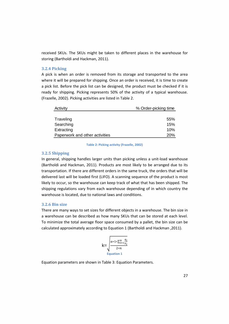
3.2.4 Picking

A pick is when an order is removed from its storage and transported to the area

where it will be prepared for shipping. Once an order is received, it is time to create

a pick list. Before the pick list can be designed, the product must be checked if it is

ready for shipping. Picking represents 50% of the activity of a typical warehouse.

(Frazelle, 2002). Picking activities are listed in Table 2.

Table 2: Picking activity (Frazelle, 2002)

3.2.5 Shipping

In general, shipping handles larger units than picking unless a unit-load warehouse

(Bartholdi and Hackman, 2011). Products are most likely to be arranged due to its

transportation. If there are different orders in the same truck, the orders that will be

delivered last will be loaded first (LIFO). A scanning sequence of the product is most

likely to occur, so the warehouse can keep track of what that has been shipped. The

shipping regulations vary from each warehouse depending of in which country the

warehouse is located, due to national laws and conditions.

3.2.6 Bin size

There are many ways to set sizes for different objects in a warehouse. The bin size in

a warehouse can be described as how many SKUs that can be stored at each level.

To minimize the total average floor space consumed by a pallet, the bin size can be

calculated approximately according to Equation 1 (Bartholdi and Hackman ,2011).

k=

Equation 1

Equation parameters are shown in Table 3: Equation Parameters.

Activity % Order-picking time

Traveling 55%

Searching 15%

Extracting 10%

Paperwork and other activities 20%

28

K= the depth of the bins

=order quantity

= stack height in number of SKUs

n= number SKU´s

a= aisle width

Table 3: Equation Parameters

3.2.7 Warehouse Management System

Some warehouses of today are very large and complex. A warehouse could contain

thousands of SKUs and could have many employees. WMS is a complex software. It

keeps track of all the storage locations and helps managing the inventory. The WMS

will make sure that everything is handled and picked correctly and as fast and

efficient as possible (Bartholdi and Hackman, 2011). The WMS knows about every

product which is stored in the warehouse. It knows the dimension, the quantity and

all other important information regarding the product. With this information, it is

possible to coordinate the warehouse operations in a very efficient way.

The WMS will prepare a picking list for the pickers to decrease the picking time as

much as possible. The WMS can also consolidate different orders with each other to

create savings. Due to the WMS, the pace in the supply chain has increased greatly

in the last 20 years (Bartholdi and Hackman, 2011). Accurate, controlled product will

move faster in the supply chain and give better service to the customer. It will also

decrease the lead-time for inventories in the system.

Basic features of most WMS’s include tools to support (Bartholdi and Hackman,

2011):

Appointment scheduling

Receiving

Quality assurance

Put-away

Location tracking

Work-order management

Picking

Packing and consolidation

Shipping

3.3 Warehousing Costs All activities in a producing company create a cost. Two main cost groups are taken

into account; the Life Cycle-Cost and The Warehousing Cost. The general definitions

29

are first presented. Thereafter, the cost definitions for the Arganda factory are

presented which will be used when comparing the different scenarios.

3.3.1 Holding Costs

By keeping a stock, capital is tied up which could have been invested or kept in the

bank with a return of interest (Axsäter, 2006). Therefore, the keeping of stock will

contribute to a potential loss of revenue (Oscarsson et al, 2006). This capital cost is

often the major part of the total holding cost. Other costs could be obsolescence,

insurance, waste and damages (Oscarsson et al, 2006). The holding cost is usually

presented as a cost per unit and time.

3.3.2 Handling Costs

The Warehousing and Handling cost are all the costs related to operate a

warehouse. All costs for personnel and transport within the facility are included in

the warehousing cost (Oscarsson et al, 2006). In addition, the building itself creates

costs such as heating, maintenance etc. There are costs related to the handling of

the arriving goods as well as the departing goods. Receiving, putaway, picking and

shipping are examples of activities creating a handling cost.

3.3.3 Life-Cycle Cost

Throughout the life time of a product, there will be a number of costs which the

product is accounted for. First of all, there are costs involved when it comes to the

development and research of a new and/or existing product. Once developed, it will

take the next step in the life cycle; the production. It starts with base material and or

semi produced components which have to be ordered. Thereafter, the base material

will be transported to the production site, where it will be refined in a number of

different activities. If the manufacturing of the product requires many activities,

sometimes buffers or WIP-stock must be held. The manufacturing will finally be

finished and the product will be transported. It can be transported directly to the

customer or to a DC where it will be stored and later on distributed. Finally, the end-

consumer will purchase, use and dispose or recycle the product. The general life-

cycle of a product can be seen in Figure 12.

30

Figure 12: Life-Cycle Cost

Each activity in a factory chain is related to a cost. By decreasing a cost of an activity

without considering the effect on the other activities in the factory chain, the result

may be a sub-optimization with an increased total cost (Stock and Lambert, 2001)2.

The total cost can only be reduced by using the systems approach, which is a more

holistic approach to the entire system where sub-optimization is not performed

(Stock and Lambert, 2001).

3.3.4 Cost Definitions Arganda factory

The total holding cost in Arganda: can be calculated by taking the average inventory

level in the model multiplied by the average stay time in racks for the warehouse.

The handling cost: will be calculated and compared. Relocation is when a SKU is

moved if blocking an ordered SKU. By multiplying the handling cost with the

relocation factor, the cost for unnecessary movement will be revealed. The handling

cost is distributed between the material handling activities; receiving, put-away,

picking and shipping. 50 % of the total handling cost can be associated with the

picking activity. Relocation only occurs in the picking activity. As seen in Table 2, the

picking activity is divided into different sub-activities. Therefore, it is assumed that

the Relocation Cost is 50 % of the picking cost or 25 % of the Handling cost.

2 Referring to Joseph Cavinato: “a total cost/value model for supply chain competiveness”

Journal of Business Logistics 12no. 2 1992 pp 285-301

31

The travelling cost for the forklifts is 55 % of the picking activity. Assuming that the

cost is evenly distributed over the different sub-activities, the travelling cost is set to

55% of the picking cost. This assumption results in that the travelling cost is 27.5 %

of the Handling Cost.

The cost equations can be seen in Table 4: Cost Equations.

Relocation cost (RC) = 25% of handling cost = 15.7/4 = 3.93€

Total RC per day = RC per SKU * Average amount of Relocations per day

Annual RC = 50 weeks*5 days*Total RC per day

Total Holding Cost (HC) per day = Average Inventory level* stay time(days) per SKU * HC

Annual HC = 50 weeks*5 days*Total HC per day

Annual measured Cost = Annual HC + Annual RC

Travel Cost per meter =

Average Travel distance per SKU

=

Total Travel Cost per day = Travel Cost per meter*Total Travel Distance/7

Annual Travelling Cost = 50weeks*5days a week* Average traveling cost per day

Table 4: Cost Equations

33

4. Finished Goods Inventory Description

This chapter will include a system description of the FGI in Arganda. The layout will

be described as well as the SKU flow process. The stakeholders will be presented and

the key stakeholders more thoroughly described.

4.1 Layout The warehouse in Arganda divided into three main areas; FGI, WIP and Additional

Material. Each area is accessible through gates where the forklifts can drive and the

pedestrians can walk. In Figure 13, the three main areas are visualized.

Figure 13: Layout Warehouse Arganda

4.1.1 Finished Goods Inventory

The Finished Goods Inventory has different capacity in the bins. A pallet position represents the floor space occupied by a SKU. The bins have capacity from 6-30 numbers of SKUs. There is also a Vendor Managed Inventory (VMI) section in closest region to the loading bay area which is used from time to time. Figure 14 shows the bin layout of the FGI.

34

Figure 14: Bin Distribution Arganda

The bins have a width of 1500mm. This means that there is additional space in each

bin when a SKU is stored there hence to the width of a SKU which is 1150mm. The

additional space enables a person to walk between the bins to look when a certain

SKU has to be located. The forklift drivers are instructed to place all SKUs to the left

in each bin to create the additional space. This can be seen in Figure 15.

Figure 15: Bin width

The most common size of a bin is three pallet positions and the least common size is

ten pallet positions. The total FGI capacity is summarized in Table 5.

Additional space

35

Bins

SKU Capacity / Bin Number of Bins Total SKU Capacity 30 3 90 27 6 162 24 8 192 21 6 126 18 16 288 15 12 180 12 4 48 9 38 342 6 21 126

114 1554* Table 5: Bins FGI

There is no dedicated pre-staging area in the FGI in Arganda. The loading bay area is

only used during the night as a pre-staging area, for the morning shipments to the

external warehouse. The forklift driver get a picking list from the administration

department and are supposed to pick the order and deliver it directly to the truck

driver, which will load it on the truck himself. Table 6 shows the specification of the

FGI:

FGI Arganda

Maximum capacity 1554 SKUs Average in stock 1200 SKUs Weekly turnover 3000 SKUs Daily throughput 600 SKUs Throughput time 2 days

Table 6: Material Flow Arganda (José Maria Escrich 2012)

*When each pallet position stores three SKUs

36

Main Aisle: There is a main aisle, see Figure 16, in the middle of the FGI which is

heavily trafficked and 5 smaller crossroads where additional bins can be reached.

Figure 16: Main Aisle seen from Loading Bay Area

The main aisle has two-way traffic and forklifts can meet without yielding. If a SKU is

picked from a bin with entrance from the main aisle, other forklift drivers give way

for the picking forklift. Pedestrians can walk within the restricting lines in the main

aisle.

4.2 Storage Keeping Unit The SKU consists of a wooden pallet, with different amount of reels of packaging material on it, see Figure 17. The SKU is wrapped in plastic to prevent any damage during transport or storage. The SKU has a label with all the necessary information. The dimensions of the pallet are not the traditional Euro pallet dimensions. There are seven different types of reels that could be stacked on a SKU. These different types are related to the size of the carton package which will affect the width of the reel. The standard sized SKU has five reels and weighs approximately 1100 kg. Dimensions:

Pallet dimensions: 1150x1150x140 mm

The maximum allowed height of a SKU is 1755mm (including the pallet)

The minimum height of a SKU is 320mm (including the pallet)

The average dimension of a SKU is 1670mm

Average number of reels on a pallet is 5.

37

Figure 17: SKU

4.3 SKU Flow Process The FGI in Arganda operates 24 hours a day, 5 days a week since there are only

arriving SKUs from Monday morning to Saturday morning. The picking process is

only operating 12 hours per day 08.00-20.00, 5 days per week.

Finishing Area

The Finishing Area is the last step in the production process. The mother rolls arrive

there after being printed and laminated. At the Finishing Area, the mother rolls will

be mounted in a slitting machine and divided into reels containing a single row of

packages, see Figure 18. The reels are thereafter stacked on a pallet and transported

to a plastic wrapper. Today, there is a major project which involves the rebuilding of

the Finishing Area in Arganda. This has had some impact on the FGI; The Automated

Guided Vehicles (AGVs) have a significantly shorter distance to travel to unload in

the FGI compared to before the rebuilding. One of the results is that there are less

AGVs able to queue up for unloading in the FGI than before. Another result is that

sometimes the AGV fail to pick the SKU from the plastic wrapper due to errors in the

new programming. The outcome is that the forklift drivers have to manually pick the

SKU instead of the AGV from the plastic wrapper. The Finishing Area operates

Monday to Friday, 24 hours a day. The last shift ends on Saturday morning at 6 am.

6 reels on a pallet

38

Figure 18: Slitting Process

Transport to Finished Goods Inventory

Each time a SKU leaves the Finishing Area, it will be logged in the factory master

computer. The data consists of all relevant data for each SKU such as number of

reels, height of a reel, reel diameter etc. See Appendix III for detailed data. Each

production order has a unique number which represents the quality and type of

packaging material the specific customer has ordered.

Once the SKU is wrapped in plastic and labeled in the Finishing Area, it is picked up

and transported to the FGI by an AGV, see Figure 18:1. When the AGV arrives to the

FGI, it places the SKU on a conveyor belt with a total capacity of five SKUs, see Figure

19:3. If the maximum capacity is reached, the AGVs will queue up outside the FGI.

The AGVs are always prioritized regarding the traffic occurring between the Finishing

Area and the FGI. This means that pedestrians and forklifts will wait until the AGVs

have passed. The number of AGVs is 20 in Arganda, but not all the AGVs transport

SKUs to the FGI. The AGVs has different task along the whole production. However,

the transport to the FGI is a prioritized task for the AGVs. In general, there are 5-10

AGVs transporting SKUs to the FGI.

Figure 19: Transport to FGI

Conveyor Belt

39

Receiving

Once the SKU has arrived to the FGI, it will be placed on a 6m long conveyor belt

which has a speed of approximately 0.2 m/s. There is a delay time between that the

AGV has placed the SKU on the conveyor belt and when the conveyor belt will

actually start transporting the SKU. This safety delay will guarantee that the AGV has

exited the receiving zone. Once the SKU has reached the endpoint of the conveyor

belt it is received by a forklift, see Figure 20. The forklift driver picks the SKU and

scans the barcode of the label. The data received provides relevant data regarding

the SKU; order, batch, what type of text is printed and so on. The data is loaded into

a WMS system called Witron. For the first SKU in an order, it automatically suggests

an available bin in the FGI. The forklift driver has to decide if the suggested bin is

appropriate for the current order size or not. For example, if the suggested bin is too

small for the order, a larger available bin is chosen. The forklift driver manually

changes the bin in the WMS- system. The WMS-system will then suggest the

manually chosen bin for the following SKUs in the same order.

Figure 20: Conveyor Belt

Put-away

The SKU is placed in the chosen bin once it has been received and scanned, see

Figure 21. The maximum height of the stacked SKUs in the warehouse is not allowed

to be higher than 5300 mm due to insurance policies. The standard SKU size is 1670

mm which allows a stacking number of three. If the SKUs are to be transported in a

container, the SKUs have a lower height, approximately 1060 mm. This allows the

SKUs to have a stacking number of five in the warehouse. The reason for the lower

height is that in a standard container with a height of 2400mm, the stacking number

is two.

40

Figure 21: Put-Away of received SKU

There is another constraint regarding the stacking. All SKUs are not allowed to be

stacked on each other. The bottom deck board must be able to distribute the weight

of the pallet, see Figure 22. To guarantee a safe working environment, a study has

been made in this field (Escrich, 2012). The study showed that the top reel diameter

cannot be smaller than 975 mm.

Figure 22: SKU stacking

Pallet bottom deck board

Top reel

41

Picking

The forklift driver receives a picking list from the shipping office with which order

and the amount of SKUs that are to be loaded on the awaiting trucks or containers.

The forklift driver picks the SKU and immediately scans it as “picked”. This will

inform the WMS-system that the SKU is no longer in stock. Since the FGI has lanes

with mixed orders due to lack of space, there is a chance that the SKU that will be

picked is blocked by other SKUs. If that happens, the forklift driver has to find

another available bin to place the blocking SKUs in. Each SKU that is moved will be

scanned and the new bin location is updated in the WMS-system. Once the SKU is

picked according to the picking list, it is transported to the loading bay area.

Loading

When the SKU is picked and transported from the bin, it will be unloaded in the

loading bay area, see Figure 24. Thereafter, it is picked up by a pallet truck (Figure

25) and placed inside the truck or container. Some deliveries also require additional

material such as plastic polymers which are used in the ejection molding of the caps.

The additional material will then be shipped together with the packaging material.

There are three loading docks which can be used simultaneously, see Figure 23. One

of the docks can be used for both containers and trucks while the other two docks

are only used for trucks. The trucks and containers are docked at a first-come-first-

served basis unless it is a rush order. The trucks to customers are only loaded 08.00-

20.00. This gives the evening shift time to pre-stage two truckloads in the loading

bay area for the following morning. These trucks will arrive at 06.00 in the morning

and will depart for the external warehouse in Azuqueca de Henares. Consolidation of

different customer orders in the same truck or container is not applied when

transporting to the customer. It is only applied when transporting to the external

warehouse to have as many full truckloads as possible. It takes approximately 10

minutes between the undocking of the first truck until the start of loading the

following truck. During this time, the first truck will exit the docking area and a

waiting truck will enter the loading area to dock. Once the truck has been docked,

the truck driver will hand over the shipping documents. Thereafter, the loading of

the truck can begin.

42

Figure 24: Loading Bay Area

Figure 25: Pallet Truck

Figure 23: Loading Docks

43

4.3.1 SKU Flow Chart Finished Goods Inventory

Figure 26 presents each step in the SKU process and all the concerned activities. The

flow chart is presented on the next page. The following steps and decisions have

been identified:

1. SKU arrives to the FGI and placed on a conveyor belt

2. The SKU is transported by the conveyor belt to the receiving location.

3. Is it a rush order?

3a. YES.

The SKU is not scanned and are transported directly to the loading

bay area.

3b. NO.

The SKU is picked up and scanned.

4. The WMS-system suggests a random place in the warehouse.

5. The receiving forklift lift driver decides if the SKU should be placed in the

recommended bin or to choose another bin.

6. The SKU is placed in the chosen bin.

7. The receiving forklift driver updates the WMS -system where the SKU has

been placed

8. A picking list is delivered to the picking forklift driver by the shipping office.

9. The picking forklift driver arrives to the given bin to pick up the SKU.

10. Is there other pallets blocking the picking for the SKU?

10a. YES.

He picks up the other SKUs and places them in another bin and

updates the WMS - system where the SKUs have been replaced.

10b. NO.

He picks up the SKU and scans it.

11. SKU is transported to loading area

12. SKU is placed in the loading area

13. Is the shipping associated with a container?

a. YES

One of the picking forklift drivers will do the loading of the container.

14. Pallet is picked by truck driver

END: Pallet is placed in the truck or container.

44

start

1

3

2

3b3a

4

5

6

7

8

9

10

10b10a

11

12

13 13a

14

End

NOYES

NOYES

YES

NO

Data

Data

Figure 26: SKU Flow Chart Arganda

45

4.4 Stakeholders Each stakeholder influencing the system must be identified as well as which level of

involvement they have. By discussing with personnel working in the FGI and the

responsible managers, all relevant stakeholders have been identified. Figure 27 is

visualizing the level of influence the stakeholders have on the FGI.

Figure 27: Stakeholders

The inner circle is representing the system. Forklift drivers, Warehouse Support and

Forwarders are all involved in the activities that are directly related to the

improvements that will be analyzed in the simulation of the FGI. The middle circle

contains the Customers, Logistics Control Tower and Market & Sales which all have

an indirect influence on the FGI due to order and shipping size. The outer circle

represents the Company as a global company which will benefit by having lower

costs and an additional part in their simulation model library. Forklift Drivers,

Forwarders, Customers and External Warehouse will be more thoroughly described.

46

4.4.1 Forklift Drivers

The forklift drivers are the vast majority of the personnel working in the FGI. They

have been separated into two teams; Picking and Receiving. The average salary for a

forklift driver is 36 400€ per year (Escrich 2012).

The Receiving team of two forklift drivers is handling the receiving and put-away of

the SKUs. In addition, they also supply the Production with aluminum foil and supply

the Finishing Area with empty pallets. A light will be turned on in the FGI receiving

area when pallets or aluminum is needed. It takes about 5-10 minutes to supply the

Finishing Area and it has to be done approximately 15 times per shift. The supplying

of aluminum foil takes about 15 minutes and has to be done four times per shift.

However, the production does not always use aluminum in the production (Garcia,

2012). The receiving team working hours can be seen in Table 7.

Working hours Receiving team

Monday - Sunday

Shift 1 07.50 – 15.50

Shift 2 15.50 – 23.50

Shift 3 23.50 – 07.50

Table 7: Working hours receiving team

The shifts are overlapping each other with 10 minutes so usually the forklift drivers

arrive to the FGI 10 minutes before the shift starts. Each forklift driver is entitled to

one hour break per shift. It is usually divided into a larger break, 30-40 min, followed

by smaller 10 minute breaks. At night, the receiving shift is losing one man-hour due

to covering for other forklift drivers working in the WIP inventory or BMI when they

have breaks (Garcia 2012).

The Picking team is assigned to pick and transport the SKUs according to the picking

list. In addition, the team is also loading containers. One of the forklift drivers is

always assigned to unload trucks with empty pallets and cores3, put-away the empty

pallets and cores and finally supply the production with empty cores. The Picking

team has an overlapping shift with one additional forklift driver during the peak

hours of truck arrivals. Each forklift driver is entitled to one hour break per shift. It is

usually divided into a larger break, 30-40 min, followed by smaller 10 min breaks.

The picking team working hours can be seen in Table 8.

3 A core is a tube of corrugated cardboard where the packaging material is rolled up on.

47

Working hours Picking team

Monday – Friday

Shift 1: 3 forklift drivers 07.50 – 15.50

Shift 2: 1 forklift driver 11.00 – 19.00


Table 8: Working hours Picking team

4.4.2 Forwarders

All shipments from the FGI are made by road. The load carrier is either a truck with a

trailer or a truck carrying a container. The container can be transported to a harbor

for further transportation by sea. The trailer is usually delivered directly to the

customer.

Containers: All containers are loaded by the Company FGI personnel. When the

standard container-SKU is loaded in the container, the stacking number is two

except for Japan, where the stacking number is one. Since the shipment will go by

sea, there are number of safety measures to apply. To avoid moist and mold in the

pallets, moisture absorbing bags are placed underneath the pallet. To avoid the

stacked SKUs to tip over or be knocked in to the container wall, large air bags are

placed to protect the SKUs. In addition, all SKUs are strapped tightly and secured.

These additional measures contribute to a longer loading time and increased

workload for the fork lift drivers. A container takes approximately 1-2 hours to load

depending on the amount of SKUs loaded. A container must be loaded within three

hours from the agreed shipping time. Otherwise, Company will have to pay a fee of

45 euro/hour. SKUs are loaded in both 20 ft (Figure 28) and 40 ft containers, but the

40 ft container is more common.

Figure 28: 20ft container

48

The container dimensions can be found in Table 9 (Ocean Container dimensions,

2012).

Container 20 feet 40 feet

Inside Height 2.38m 2.38m

Inside Width 2.33m 2.33m

Inside Length 5.89m 12.01m Table 9 Container dimensions

These dimensions and with the stackability of 2 will lead to 20 SKUs in a 20 ft

container. The 40 ft container has a max capacity of 40 container-sized SKUs, but

due to weight constraints, it will only be loaded with approximately 36 SKUs.

Trailers: All trailers are loaded by the truck drivers. The domestic customers have

their own trucks. The international transports are ordered through the Logistics

Control Tower who orders the trucks from different forwarders. A trailer can load 22

standard SKUs which will not be stacked. When loaded with 22 SKUs, the truckload is

close to the maximum weight allowed which is 24 tons. It takes approximately 30

minutes to load a trailer. If it is an international shipment, the SKUs have to be

secured with protective material to avoid transportation damages. Once the trailer

has been docked to the loading bay area, it must be loaded within 2 hours or a fee of

35€ per hour is debited (Escrich, 2012).

The dimensions of a trailer can vary, but the most common is the one presented in

Figure 29.

Figure 29: Standard Euroliner Truck (Standard Lastbilsflotta, 2012)

49

4.4.3 Domestic Customers

The domestic customers are applying VMI – system. This means that the customers

are updated regarding their orders as soon as they have been produced. The

information sent is how much of their orders that are placed in the FGI and how

much of those are placed in the external warehouse. Since the domestic customers

are 65% of the total shipments, they have a large influence (Escrich 2012). No

delivery order has to be placed by the domestic customers and since the VMI is

used, the customer trucks arrive whenever there is a need for packaging material.

This situation makes it difficult for the shipping office to plan the loading in advance.

The lead time, which is the time from an order is placed to Estimated Time of

Dispatch (ETD), is 14 days and the invoice is sent as soon as the order has been

produced. The domestic customers places larger orders compared to the

international customers and the orders are stored significantly longer in the FGI. This

is a result of the use of the VMI-system in a combination with that the invoice is sent

directly when the order is produced. The customer can therefore use the FGI to

store their own goods as long as possible.

4.4.4 International Customers

The international customers are approximately 35 % of the total shipments, where

25 % are delivered to Portugal and the remaining 10 % to the rest of the world

(Escrich, 2012). Each customer places a delivery order when the production order is

placed. This will make it possible for the shipping office to order trucks from the

Logistics Control Tower. The lead time, order – ETD, is 14 days and the invoice is sent

when the truck has been loaded and dispatched. A security guard ensures that all

documents are in order and that nothing else is loaded on the truck except what is

on the shipping list.

4.4.5 External Warehouse

About 200 SKUs of the total daily shipments goes to an external warehouse in

Azuqueca de Henares which is located 46 km from Arganda. This warehouse has an

additional capacity of 4800 SKUs. This warehouse also supplies the factory in

Arganda with raw material goods multiple times a day by truck loads. Approximately

50 % of these trucks return to the external warehouse with finished goods in order

to save transportation costs (Escrich, 2012).

50

4.5 Key Performance Indicators The FGI in Arganda is evaluated with the following KPIs:

Perfect Delivery

o Order delivered on time

o Order delivered in full

Inventory Level

The Perfect Delivery contains both order delivered on time and order delivered in

full. Order delivered on time was until recently measured at the ETD. Order

delivered in full has a ±5 % deviation from the actual order size to be considered full.

51

5. Simulation Model

This chapter contains a detailed description of how the simulation model has been

constructed with all the different processes. The result from the validation of the

model will be presented as well as improvement scenarios which will be part of the

experiments.

5.1 Model Description The model represents a non-terminating system, which means that there is no

specific stop when the simulation is over. Since there are no incoming SKUs during

the weekend and no departing SKUs either, the weekend will not be part of the

simulation. Figure 30 shows an overview of the complete model of the FGI and the

AGV path from the Finishing Area.

Figure 30: Overview of Simulation Model

5.1.1 Layout Finished Goods Inventory

A digital blueprint of the FGI is used for the model to obtain the correct

measurements. The current layout of the FGI is used in the model. In the model, the

FGI will be structured by 27 different floor storage zones which represent the

different areas of bins. The bins are divided into pallet positions, which are the

squares in the floor storage zones seen in Figure 31. The pallet position that the SKU

is placed in has the dimensions of 1150*1500 mm and the stacking number depends

totally on the height and diameter of the SKUs.The high amount of floor storage

zones will increase the accuracy when a SKU will be relocated due to blocking SKUs.

SKUs can therefore more easily be sent between the different objects based on the

Exit

Finishing Area

Vehicle Path

52

need of relocating SKUs. The light coloured floor storage zones are entered from the

side aisles and the dark coloured floor storage zones are entered from the main

aisle.

Figure 31: Layout FGI

5.1.2 Storage Keeping Unit

The completion of the SKUs is performed at the exit of the Finishing Area. Reel by

reel will be stacked on a pallet. The data for the generated reels consist of all

relevant information regarding how many reels should be stacked on each pallet as

well as the height of each reel etc. For a complete view of input data, see Appendix

III. The SKUs consisting of wooden pallets with reels of packaging material will be the

flow item in the simulation model. One production order can contain variety of

SKUs. The SKU is always accessible for the forklift. The maximum diameter is set for

the reason to make sure that the reels on the pallet do not reach outside the frame

of the pallet. The SKUs that belongs to the same production order will get a specific

colour. The colour simplifies the identification when the animation is watched and

the stacking is controlled, the SKUs with the same colour should be stacked

together. A virtual SKU is visualized in Figure 32.

Floor storage zones

Entry FGI

Exit FGI

53

Figure 32: SKU

When stacking, the minimum diameter allowed for the top reel of the SKU is 975

mm hence to the dimensions of the bottom structure of the wooden pallets. If the

top reel diameter is any smaller than 975 mm, the stacked SKU will not be

considered stable and has an increased risk of tipping over. The SKU dimensions can

be seen in Table 10Table 10: SKU dimension.

SKU

Max height 1755mm Min height 320mm Max diameter 1150mm Pallet size 1150*1150mm

Table 10: SKU dimensions

5.2 SKU Flow Process Transport to Finished Goods Inventory: The SKU is collected at the exit of the

Finishing Area. Thereafter, it is transported to the entry of the FGI. All other vehicles

and pedestrians give way for the AGVs when they are transporting from the

Finishing Area to the FGI. The AGVs will follow a path with a single capacity; the

vehicles cannot pass each other. The path, pickup point at the Finishing Area and the

exit at the FGI are seen in Figure 33.

54

Figure 33: Transport to FGI

Receiving: In the receiving area there are two forklifts working during each shift.

The SKU is placed on the receiving conveyor belt. The conveyor belt has a safety

delay time of approximately 30 seconds that starts directly when the SKU is put-

down on the conveyor belt. However, in the model there will be a longer unloading

time for the AGV instead of a safety delay time. The virtual receiving activity is

visualized in Figure 34.

Figure 34: Receiving of an SKU in the FGI

Finishing Area Exit

FGI Entry

Arriving SKUs

55

The conveyor belt has a length of 6 meters and a speed of 0.2 m/s. The conveyor

belt will have no breakdowns in the simulation model. After transportation on the

conveyor belt, the SKU is ready to be picked by a forklift. The forklift picks the SKU

from the conveyor belt. Each pick from the conveyor belt including the scanning of

the SKU, is simulated with a triangular distribution of [11, 24, 16]4 seconds.

Put-away: The logic code will trigger when the SKU is on the conveyor belt and it will

decide the location for the SKU in the FGI. The logic code is designed to behave as

the WMS for the FGI as much as possible. It will first check if there are any matching

SKUs with the same Production order ID in the FGI and try to place on top without

exceeding the height constraint. The virtual Put-away activity is visualized in Figure

35, where the height constraint is not reached.

Figure 35: Put-away a SKU in a stack

No mixing of the production orders is allowed at the same pallet position. If the

height constraint is reached, the logic code checks if the SKU can be placed in front

of the matching SKUs. If not, the SKU is placed in an empty bin or the bin with most

available pallet positions. If there is no matching order or there is no pallet position

4 In a triangular distribution the first value is the minimum time, the second value is the most

common time and the third value is the maximum time.

56

nearby, it will first check if there is an empty bin to place the SKU in. If there is no

empty bin, it will place the SKU in the bin with most empty pallet positions. The total

height of a stack cannot be higher than 5300 mm. The top reel diameter cannot be

smaller than 975 mm if stacking should be allowed. The unloading sequence will be a

mean of the time it takes for unloading at different heights. When the FGI becomes

full, the arriving SKUs will stay on the conveyor belt until there is an available pallet

position. After a put-away, the forklift returns to the receiving area. An assumption

is made due to the order size. The model does not take the order size in

consideration when suggesting a pallet position.

Picking: Historical data of the picking orders will be used which will generate an

event. One forklift driver has been removed from Shift 1 and Shift 3 due to unrelated

work activities of the picking process. The forklift driver is told to drive to a specific

location and pick up the ordered SKU. If another forklift is blocking the way by

picking or put-away activities, the last arriving forklift has to wait until the first

forklift is finished with the put-away or picking. This will be modelled by a

temporarily block that will be set on the bin for the other forklift drivers.

When a picking list arrives, it is possible that the SKUs which are included in the

picking list are blocked by other SKUs. If this would happen, the blocking SKUs must

be relocated somewhere else in the FGI. The picking list arrives to the queue in front

of the truck. At the same time as the picking order enters the queue, the logic code

for the queue starts and checks if there are any SKUs in the FGI with the same

production order ID as on the picking list. If a SKU with the same production order ID

is found, the logic code checks if there is any SKU in front of the ordered SKU. If

there is a SKU blocking, another logic code starts which is similar to the logic for the

putaway activity. It will first check if there are other SKUs with the same production

order ID as the blocking SKU. If so, the blocking SKU will be placed there. If there are

no similar SKUs, the blocking SKU will be placed in an empty bin or in the bin with

most empty pallet positions. When the SKU is relocated, it sends a message to the

truck and triggers a logic code to check if there are more SKUs blocking the SKU

which is to be picked. In the relocation process, the height and top reel diameter

constraint are taken in consideration as well. This process goes on until all the

blocking SKUs are relocated and the ordered SKU can be picked. Virtual blocking

SKUs can be seen in Figure 36.

57

Figure 36: Blocking SKUs when picking ordered SKU

When the forklift picks up the blocking SKU for relocation, the current bin will be

blocked so no other forklift can place other SKUs in that bin. When all SKUs have

been relocated, the ordered SKUs can be picked. A label is put on the floor storage

zone meanwhile the forklift is relocating a SKU. The logic code for relocating is

programmed to compare the suggested bin for relocating a SKU to the label on the

floor storage zone. If there is no match, the SKU can be placed in that bin.

Loading: Once a SKU is picked, it is transported and unloaded in the loading area.

The SKU is placed in a FIFO queue at the correct loading dock. During 08.00-20.00,

there is one person, or resource, for each loading dock simulating the truck driver.

Containers will not be part of the model since no historical data regarding the arrival

frequency have been received.

Loading time for a trailer is shown in Table 11.

Load carrier Capacity (SKU)

Loading time (min)

Trailer 22 20-40 Table 11: Loading Data

Ordered SKU Blocking SKUs

58

No pallet truck will be part of the model since it is considered having walking speed

of 1.4 m/s which is the same speed as the human resource (Preferred walking speed,

2012). The two truckloads that are pre-staged during 20.00-23.50 will not be

performed in the model. Instead the picking and loading will start earlier in the

morning to compensate. Once a picking list has been completed, there will be a

delay for the next picking order to arrive. Since the trucks are assumed to arrive

independently of each other, the arrivals can be assumed to follow a Poisson

process with an exponential inter-arrival time (Marklund and Laguna, 2005). This will

symbolize the undocking and exit of the current truck and enter and docking of the

waiting truck. No loading of additional material will be included in the model. The

loading process is illustrated in Figure 37.

Figure 37: Loading of SKUs on trailers at the loading docks

59

5.2.1 Arrival SKU Process

There are many events which can occur and decisions that are made during the

arrival process. Figure 38 is a detailed flow chart of the events in reality related to

the arrival process of a SKU. The arrival process in the model is mainly based on

these events and decisions. A detailed description of the decisions and events in the

flow chart is given:

Start: SKU enters the pick point of the Finishing Area 1. Available AGV?

Yes: AGV prepares to pick SKU No: Add one SKU to a queue

Wait until an AGV is available. AGV prepares to pick SKU

2. AGV picks SKU 3. AGV transports the SKU to the receiving conveyor belt of the FGI 4. Another AGV unloads on the Receiving conveyor belt?

Yes: AGV is placed in a FIFO queue Wait until the other AGV has unloaded. AGV prepares for unloading on the receiving conveyor belt

No: AGV prepares for unloading on the receiving conveyor belt 5. AGV checks if conveyor belt is full 6. Is the conveyor belt full?

Yes: AGV waits until there is an empty slot on the conveyor belt to unload the SKU

No: AGV unloads the SKU on the conveyor belt 7. SKU is located on the conveyor belt 8. Conveyor belt starts to transport the SKU 9. Any other SKU on the conveyor belt?

Yes: SKU is transported on the conveyor belt to the preceding SKU. FIFO queue is created

No: SKU is transported to the pick point at the end of the conveyor belt 10. SKU reaches the pick point at the end of the conveyor belt 11. Is there an available forklift?

Yes: forklift driver prepares to pick and scan the SKU No: SKU waits at the pick point until there is an available forklift

Forklift prepares to pick and scan 12. Forklift driver picks and scans the SKU 13. First SKU in an order?

Yes: Forklift driver transports the SKU to the suggested bin by the WMS-system

14a. Forklift driver arrives to the suggested bin 15a. Bin size appropriate?

60

Yes: SKU placed in the suggested bin END No: Appropriate bin is manually chosen

by the forklift driver. No: Forklift driver transports the SKU to the pre-chosen bin 14b. Forklift driver arrives at the bin

15b. Is the bin full? Yes: Forklift driver chooses to place the SKU in the closest available bin 16. Forklift driver places the SKU in the bin No: Forklift driver places the SKU in the bin

END

start

1NO

YES

FIFOQueue

2

3

4

NO

YES FIFOQueue

5

6

NO

YES7

7

FIFOQueue

8

9

NO

YES

10

FIFOQueue

11

YES

12

FIFOQueue

NO

13 NOYES

14a

15a

YES

End

14b

15bYES

NO

16

NO

Figure 38: Arrival Process

61

5.2.2 Departure SKU Process

Figure 39 is a detailed flow chart of the events related to the departure process in

reality of a SKU. The departure process in the model is mainly based on these

decisions and events. Each step is described in detail:

Start: The forklift driver gets a picking list.

1. The forklift driver drives to the bin according to picking list.

2. Are there some other forklift picking SKUs that prevent his transportation?

YES: The forklift driver will have to wait until the other forklift is finished.

The transport continues

NO: The forklift driver continues his transport.

3. Forklift driver arrives at the bin according to picking list

4. Is there some other SKU that block the chosen SKU from picking?

YES: The forklift driver scans and removes the blocking SKU and places it in a

near bin

(This activity is repeated until the first condition is false)

NO: He scans and picks up the SKU

5. Forklift driver transport the SKU to the loading area.

6. Are there some other forklift picking SKUs that prevent his transportation?

YES: The forklift driver will have to wait until the other forklift is finished.

NO: The forklift driver continues his transport.

7. SKU arrives in the loading area

8. Are there anything blocking the unloading in the loading area?

YES: The forklift driver waits until unloading is possible

Forklift driver places the SKU in the loading area

NO: Forklift driver places the SKU in the loading area

9. SKU is placed in the loading area

10. Is the shipping associated with a container?

YES: Another Company forklift driver picks the SKU with a pallet truck and

transports it to the container

11a. SKU is placed in a container.

END

NO: The truck driver picks up the SKU with a pallet truck and transports the

SKU to the trailer.

11b. SKU is placed in trailer.

END

62

Figure 39: Departure Process

start

2

NO

YESDelay

3

4

NO

YES New bin

5

11b

1

6

NO

YESDelay

7

8

NO

YESDelay

9

10 NOYES

11a

End

63

5.3 Transporters AGV: In the simulation model of the current system, there will be a pool of 3 AGVs

which only operates the transport of SKUs to the FGI. The times have been identified

for the AGVs by observations, which are used in the model and are shown in Table

12.

Activities

Loading 45sec Speed 1 m/s Unloading 85 sec

Table 12: AGV activities

The picking and unloading times are considered constant due to the automatic

procedure of the AGVs. No Mean Time Between Failure (MTBF) has been able to be

retrieved. Therefore, no MTBF will be used in the model. Figure 40 visualizes a

virtual AGV.

Figure 40: AGV with SKU

Forklifts: There is a total pool of 5 forklifts operating with respect to the shift

schedules. Two forklifts are always operating in the receiving team and 0-3 operating

in the picking team. The time for transportation is depending mostly on the distance

to the bin. However, the speed of a forklift will also have its affect on the

transportation time. The top speed is set to 3 m/s. There is no MTBF set on the

forklifts. Loading and unloading times follows a triangular distribution received by

observations can be seen in Table 13.

64

Activities sec

Loading [8,26,16] Speed 3 m/s Unloading [7,23,13]

Table 13: Activities Picking team

The forklift drivers are scheduled to one hour break per day, shown in Table 14.

Breaks

Break 1 30 min Break 2 10 min Break 3 10 min Break 4 10 min

Table 14:Breaks

The forklift drivers are overlapping their breaks so that there are always forklift

drivers operating in the FGI.

The receiving forklifts schedule is illustrated in Table 15.

Working hours Receiving team

Monday - Sunday




Table 15: Shift Receiving Team

The picking forklifts schedule is illustrated in Table 16.

Working hours Picking team

Monday - Friday




Table 16: Shifts for Picking Team

65

5.4 Input Data & Response

5.4.1SKU Cost

The costs for a SKU in the FGI can be seen in Table 17 (Escrich, 2012).

SKU costs

Handling Cost 15,7 €/SKU Holding Cost 0,9 €/day

Table 17: SKU costs

5.4.2 Data for Arriving SKUs

The generated data that are used in the model consists of eight days of arriving

SKUs. Since there is no production in the slitting machine during the weekend and

no trucks will be loaded either, the weekend has no effect on the FGI. The data

consists of in total 6 days of production which will be replicated to always supply the

FGI during longer runs. This means that after six days in the run, the seventh day of

arriving SKUs will actually be day one again. Figure 41 is a chart of the arriving SKUs

measured between the times 00.00 to 23.59.

Figure 41: Arriving SKUs per Day

5.4.3 Data for Departing SKUs

The departure data is based on historical raw data from 2011. The picking orders

have been sorted to match the generated arriving SKUs. For example, in the

beginning of 2011, SKUs which have been produced in 2010 can be picked. However,

the generated data only consists of SKUs produced in 2011. Therefore, these picking

orders have been removed from the data and replaced with picking orders where

654321

900

800

700

600

500

400

Day

SK

Us

Arriving SKUs per Day

66

SKUs exists. The data will be replicated to be able to perform longer runs. Relevant

information for the departure data consists of Picking Order ID, amount of SKUs to

be picked, production order ID etc. (see Appendix III). The amount of departed SKUs

per day according to 100 days historical data are shown in Figure 42.

Figure 42: Amount of Departing SKUs per Day

The average departed SKUs per day is 573 and the peak is around 750 SKUs. The

amount of SKUs shipped each day from the FGI follows a normal distribution which

can be seen in Figure 43.

Figure 43: Histogram departing SKUs

1009080706050403020101

800

700

600

500

400

300

200

Days

SK

Us

Amount of departing SKUs per day

800700600500400300

25

20

15

10

5

0

SKUs

Fre

qu

en

cy

Mean 573,4

StDev 101,3

N 101

Normal

Histogram of Departed SKUs

67

There is a not always clear correlation between the amount of departing trucks and

the departing SKUs. The reason is that not all trucks are fully loaded. 100 days of

trucks departing from the FGI has been plotted in Figure 44.

Figure 44: Amount of trucks per day

The distribution for the amount of trucks per day is shown in Figure 45. The Weibull

distribution is the most appropriate distribution, see curve in Figure 45.

Figure 45: Histogram Truck departure

1009080706050403020101

45

40

35

30

25

20

Days

tru

ck

s

Amount of trucks per day

454035302520

18

16

14

12

10

8

6

4

2

0

Trucks

Fre

qu

en

cy

Shape 6,583

Scale 35,43

N 100

Weibull

Histogram of Truck Departures per day

68

5.4.4 Response

Before the model is being developed, it is important to know what kind of response

that is wanted. Since this model has the purpose to improve the FGI with respect to

the life-cycle cost, the response must contain information which can be related to a

cost. Throughput is an important parameter which will be measured as SKUs per

day. Travel distance for the forklifts another important parameter since the longer it

has travelled over a specific set of time, the fewer amounts of SKUs will be delivered.

There is also a direct cost when the forklift driver is using the forklift. Since

relocating SKUs is a double handling, it has no value added. Therefore, the amount

of SKUs that have been relocated will also be measured. Finally, average inventory

level is measured per day which gives the utilization of the FGI and can be connected

to the holding cost.

5.5 Simulation Run

5.5.1Warm-up

The real FGI in reality is never fully depleted; there are always SKUs in stock. In the

simulation model the FGI will start completely empty and continuously replenished

throughout the week. For that reason, the simulation model will have a warm-up

time, meaning that the recording of data does not start at the beginning of the

simulation. Instead, the recording of data will start after three days of activity in the

FGI.

5.5.2 Length and Number of Runs

A run is the time the model is used, for example on run can be one week, one year

or just one day. The number of runs largely depends on the computational

capability. More runs mean additional time for each experiment but will also give a

more statistically reliable result. When analyzing the original model, the number of

runs has been set to 6 and each run is 10 days long where the warm-up time is 3 of

those days. This means that there will be 7 days of recorded statistics from the

model. The simulation starts at 08.00 in Monday morning, so one day in the

simulation is from 08.00 to 07.59 the day after. The reason is that at 07.59, the

maximum number of SKUs will be in the FGI due to the fact that no shipping

activities have occurred for 12 hours.

69

5.5.3 Simulation Response

Arriving SKUs

The arriving SKUs per day are the same for each run due to the historical data

generating the SKUs in combination with no dynamic of the AGVs. Furthermore, the

difference between the chart in Figure 46 and the chart in Figure 41, can be

explained by the simulation time; 08.00 to 07.59 compared to the generated input

data where the Arriving data is logged 00.00-23.59.

Figure 46: Arriving SKUs in Simulation

Throughput

The throughput is measured at the end of one day in the simulation; at 07.59. Figure

47 shows a chart with the average throughput per day.

Figure 47: Average throughput/day

7654321

900

850

800

750

700

650

Days

SK

Us

Arriving SKUs per Day

7654321

900

850

800

750

700

650

600

Days

Am

ou

nt

of

SK

Us

Plot of average Throughput

70

Inventory Level

The value at day 1 is recorded at 08.00; when simulation starts to record data. The

average inventory level can be seen in Figure 48.

Figure 48: Inventory level for original layout

Performance Parameters

All measured performance parameters can be seen in Table 18.

Table 18: Performance parameters

7654321

900

850

800

750

700

650

600

Days

SK

Us

Inventory level

OriginalLayoutAverage

inventory level

Number of

relocations

(95%)

Average stay

time in racks

(95%) (s)

Through-

put Total

(95%)

Forklift average

total distance (95%)

(m)

Input

(SKU)

mean 717 658 55304 5333 825585 5211

confidence 579-737 52238-58370 5271-5395 817657-833513 0

Std dev 75 2921 59 7553 0

min 558 50480 5264 818470 5211

max 773 58999 5394 838360 5211

inventory level

N=6

71

Calculated Cost for the Original Layout

The measured cost for the original Layout is presented in Table 19. See Appendix IV

for detailed calculations.

Annual measured cost 371961€

Annual relocation cost 92250€ Annual travelling cost 176461€ Annual holding cost 103250€

Table 19: Costs Original layout

5.5.4 Validation

The validation of the original model is have been made in three different ways, Face

Validation, Extreme Condition Test and Turing Test. The validation methods are

explained in Chapter 2.

Extreme Condition Test

Comparing the result of the Extreme Conditions test with the response from the

original model is seen in Table 20.

Table 20: Original Model vs. Extreme Conditions

The number of relocations average stay time has decreased significantly as

predicted. This can be explained by during this test all the limitations were removed

and all the SKUs that entered the warehouse was almost directly picked and shipped

when a complete order was located in the warehouse. The forklift distance

increased due to when the warehouse is empty, the arriving pallets are placed

closest to the receiving conveyor and the forklift have to drive a longer way in

general to pick up the SKUs when starting at the loading bay area. The throughput

will remain the same since the frequency of the arriving SKUs is unchanged. The

result showed that the system behaved as it should when all the limitations was

removed.

Average

Inventory

Level

Number of

relocations

(95%)

Average stay

time in racks

(95%) (s)

Through-

put Total

(95%)

Forklift average


(m)

Original Model 717 658 55304 5333 825585

Extreme Condition 145 7,1 16567 5323 1052473

72

Turing Test

The result from the Turing Test is presented in Figure 49. The model response is

much higher than the real output. The input data for the arriving SKUs has a high

frequency, which forces the model to extract SKUs with the same the frequency. If

not, the FGI will be overloaded. In addition, real input data for the arriving SKUs

would give a much more credible result. The conclusion regarding the result from

the Turing Test is that it could either be the input data that is inaccurate or the

model itself.

Figure 49: Turing Test

5.6 Experimental Design To be able to find an improved layout of the FGI, different scenarios have been

created. Once the simulation model has been verified and validated, it can easily be

modified to fit the scenarios where the possible improvements are included. In the

model, a large amount of parameters can be changed such as amount of forklifts,

amount of loading docks, location of pallet positions etc. A main objective is to avoid

any cost for implementing the improvements. However, if the improvement has a

cost, it could be considered if the total life-cycle cost is reduced compared to the

original layout.

7654321

900

800

700

600

500

Day

SK

Us

Model

Reality

Variable

Throughput Model vs Reality

73

5.6.1Modelled Scenarios

A set of scenarios have been created through discussion and brainstorming.

Thereafter, additional scenarios have been created by combining successful

experiments to evaluate if further improvements can be made. After discussions

with parts of the warehouse management in Arganda, the most relevant scenarios

have been evaluated.

Scenario 1: Add one loading dock

By adding a loading dock, four trailers can be loaded at the same time. By doing so,

the expected result is to reduce the inventory level and decrease the number of

relocations.

Figure 50: Scenario 1

Scenario 2: Optimum bin size, 6 pallet positions

This experiment has the purpose to see if it is more efficient in some way to use a

standard size for each bin. The most space efficient bin size was found by using the

formula in Equation 1. See Appendix IV for calculations. The result from entering all

variables into the formula gave that the most space efficient bin depth was six pallet

positions deep. The layout for the FGI was changed and all the bins were given the

size of six pallet positions. The trade-off by this change is that the total SKU capacity

Additional

loading dock

74

decreased to 1443 from 1554, but hopefully it would bring some savings by

decreasing the double handling in the FGI and the travelling distance.


Scenario 3: Vertical Rack

A small pallet shelf was installed as seen in Figure 52. The capacity of the FGI

decreased with 37 possible locations by implementing this shelf. The loss of capacity

might not be of big importance due to hopefully other savings such as less relocation

and maybe a better put-away policy.


Scenario 4: Add one loading dock and forklift

This experiment is the same as scenario 1 except that one extra forklift is added to

the picking team. The additional forklift will be put on the picking overlap schedule.

75

Scenario 5: High Capacity Layout


The layout in this experiment has been taken to its limit due to pallet positions. The

SKU capacity has increased to 1668 from 1554 because of additional pallet positions.

The interesting part will be to see if the extra pallet positions will decrease the

relocations.

77

6. Results & Discussion

This chapter contains the results from the simulation runs of the different scenarios.

The results of each scenario will be analyzed, evaluated and discussed.

The results will be based on the response from the simulations runs of the different

scenarios. For more accurate result, it is necessary to do more than one run. When

all the runs for the different scenarios are done, it is possible to compare the results

to each other.

6.1 Scenario 1: Add one loading dock This scenario has been under discussion among the members of the Warehouse

Management. During the peak hours at the middle of the day, the loading of the

trucks becomes a bottleneck. By adding a loading dock, the expected result was that

the average inventory level should decrease. The measured performance

parameters for scenario 1 are presented in detail in Appendix IV.

The model managed the picking orders much more efficient with the result of

smaller picking order queues. Comparison of the original model and the model with

an additional loading bay is seen in Table 21. A majority of the performance

parameters have been improved. The average inventory level has decreased by 12 %

which is a direct result of the significant decrease of average stay time in the

inventory of 34 %. The reason is could be because more trucks can be loaded in the

FGI at the same time and the picking activity can be started faster. The Number of

Relocation-parameter has also been decreased significantly. The reason could be

because of lower inventory level. Lower inventory level results in less mixed orders

in each bin. The Forklift average total distance-parameter has increased. The reason

is explained by the longer distance to reach the additional loading dock. The forklift

has to drive through the Additional Material inventory, to reach the loading dock.

Table 21: Comparison Scenario 1 vs. Original Model

78

The annual costs for Scenario 1 can be seen in Table 22. The annual relocation cost

has decreased compared to the Original Model due to the lower number of

relocations. The annual holding cost has also decreased due to the lower inventory

level in Scenario 1. The travelling cost has increased due to the longer distance to

reach the additional loading dock. No investment cost has to be made since the

trailers can be loaded from the side directly from ground level instead of docking to

a “real” loading dock.

Annual measured cost 329324 €

Annual relocation cost 63250€ Annual Holding Cost 59750€

Annual Travelling Cost 206324€

Investment Cost 0€ Table 22: Costs for Scenario 1

Comparison of the annual cost of the Original Model and Scenario 1 can be seen in

Table 23. The annual measured cost has been reduced with approximately 43000€.

By implementing this scenario, the life-cycle cost of the packaging material will be

affected in a positive direction.

Annual measured cost

Original Model 371961€ Scenario 1 329324€ Difference -42637€

Table 23: Comparison Original Model vs. Scenario 1

6.2 Scenario 2: Optimum bin size: 6 pallet positions Since the average order size is constantly getting smaller for each year, the bin sizes

in the FGI are not up to date. The best average bin size with respect to the average

order size in the generated input data has been calculated. Thereafter, the bin size

was implemented for all bins. The expectation was to lower the amount of

relocations. In this scenario, the bin size was set to 6 pallet positions. See Appendix

IV for detailed results of the performance parameters and calculations.

A comparison of the Original Model and Scenario 2 is presented in Table 24. The

experiment had a mixed result. The inventory level decreased with 4 % and the

average stay time decreased with 10% which will affect the holding cost in a positive

way. However, the amount of relocations increased substantially. The reason for the

79

result in this experiment was probably the reduced FGI capacity. Due to the capacity,

the forklift was given less alternatives to store the SKUs and therefore, more

relocations were necessary. Because relocations become more common, it is

obvious that the forklifts need to drive a longer way when there is much

unnecessary driving to relocate blocking SKUs. It was also noticeable that the

experiment started to fail if the warehouse capacity reached over 800 SKUs. The

relocations were too time consuming, so the FGI started to be overfull after some

time.


The annual costs for Scenario 2 can be seen in Table 25. The increased level of

relocation became too big to be able to gain any benefits. The relocation cost has

increased compared to the original model. The travelling cost has also increased due

to the longer distance the forklifts have travelled. The main improvement has been

the reduction of the annual holding cost due to lower time each SKU spend in the

FGI.




Investment Cost 0€ Table 25: Costs for scenario 2

Comparing the annual measured cost for Scenario 2 and the original model can be

seen in Table 26. Compared to the original model, Scenario 2 is not to be

recommended for implementation. The result shows that it would be more

expensive to implement this layout than keeping the original layout. There is an

increased annual cost with 14000€ which will affect the life-cycle cost of the

packaging material in a negative direction.

80


Original Model 371961€ Scenario 2 385742€ Difference 13781€


6.3 Scenario 3: Vertical Rack The managers of the warehouse in Arganda have discussed an installation of a

vertical rack for smaller SKUs with only two or three reels on. The expectations for

this scenario were that the removal of the small SKUs from the floor storage would

give more space for the higher SKUs and to utilize the space better in the FGI. See

Appendix IV for detailed results of the performance parameters.


result of the comparison is that Scenario 3 is an overall a worse alternative than the

Original Model. All performance parameters have increased and especially the

amount of relocations. The relocations increased in this experiment with 80 %. The

reason for the substantial increase of relocation could depend on the loss of pallet

positions due to the instalment of the rack. Also, the forklifts are needed to drive a

longer way when relocating smaller SKUs. Due to this matter, the receiving forklifts

will be able to fill up the FGI more compared to what is shipped. By this, a negative

trend starts and the inventory level will increase. It is only natural that the average

stay time increase together with the number of relocations and higher inventory

levels as well, because the time is spend on relocating SKUs instead of picking them.

Another explanation for the substantial amount of relocation could be a logic error

but it could not be confirmed.


The annual costs and investment cost for Scenario 3 can be seen in Table 28. The

annual relocation cost has increased dramatically compared to the original model

due to the higher number of relocations. The annual holding cost has also increased

81

due to the larger average inventory level. The travelling cost has also increased since

the orders have to be separated into small SKUs and large SKUs.




Investment Cost Year 1 1500€ Table 28: Costs for Scenario 3

Comparing the annual measured cost for Scenario 3 and the original model can be

seen in Table 29. The comparison of the Original model and Scenario 3 clearly shows

that Scenario 3 will increase the life-cycle cost of the packaging material. Therefore,

the scenario is not recommended.




6.4 Scenario 4: Add one loading dock and forklift This scenario was created to see of there could be any further improvements

compared to Scenario 1. One of the main disadvantages is that this experiment

involves a new resource which will add a cost. See Appendix IV for detailed results of

the performance parameters.

First of all, a comparison of the Original model and Scenario 4 was made. The result

is presented in Table 30. All performance parameters have been improved except

the Forklift average total distance for the picking forklifts. The average inventory

level has decreased by 13 % which is a direct result of the significant decrease of

average stay time in the inventory of 37 %. The reason is could be because more

trucks can be loaded in the FGI at the same time and the picking activity can be

started faster. The Number of Relocation-parameter has also been decreased

significantly. The reason could be because of lower inventory level. Lower inventory

level results in less mixed orders in each bin. The Forklift average total distance-

parameter has increased. The reason is explained by the longer distance to reach the

82

additional loading dock. The forklift has to drive through the Additional Material

inventory, to reach the loading dock.

Table 30: Scenario 4 vs. Original Model

The annual costs and investment cost for Scenario 4 can be seen in Table 31. The

relocation cost has decreased significantly which can be explained by the lower

average inventory level. By having a lower average inventory level, less SKUs have to

be relocated due to mixed orders in the bins. The decreased average stay time in the

FGI in a combination with the decreased average inventory level contributes to the

substantially lower holding cost compared to the original model. However, there are

additional cost compared to the original model; The salary of a forklift driver and the

rental of a forklift. The annual rental cost of a forklift has been estimated to 5000€.

As in Scenario 1, there is no investment cost since the trailers can be loaded from

the side at ground level. No actual platform has to be built.



Annual Travelling Cost 206163€ Annual Forklift driver Salary 36400€ Annual Rent of Forklift 5000€ Investment Cost 0€

Table 31: Costs for Scenario 4

Comparing the annual measured cost for Scenario 4 and the Original Model can be

seen in Table 32. The comparison of the Original Model and Scenario 4 has a small

reduction of annual measured cost of 12000€. This will affect the life-cycle cost of

the packaging material in a positive direction. Therefore, Scenario 4 is

recommended.

83


Original Model 371961€ Scenario 4 359620€ Difference -12341€


In addition, a comparison has been made of Scenario 1 and Scenario 4 to identify the

overall best scenario. The result of the comparison of the performance parameters is

presented in Table 33. There is no significant difference of the performance

parameters between the two scenarios except for the relocation parameter. In

scenario 4, the number of relocations has decreased with 8% compared to Scenario

1. The reason is assumed to be associated with the blocked bins in the model when a

forklift is either relocating or assigned to pick from a specific bin. If a SKU that will be

picked is blocked, the forklift will place the blocking SKUs in another bin. When only

using three forklifts, there is a risk of having blocking SKUs placed in front of the SKU

which will be picked to the additional truck later on. When having four forklifts, this

bin would automatically be blocked so no other SKUs could be placed there.

Table 33: Scenario 1 vs. Scenario 4

Comparing the annual measured cost for Scenario 1 and Scenario 4 can be seen in

Table 34. The result of the comparison shows that the life-cycle cost for the

packaging material will be annually 30000€ lower for Scenario 1 compared to

Scenario 4.


Scenario 1 329324€ Scenario 4 359620€ Difference 30296€

Table 34: Comparison Scenario 1 vs. Scenario 4

84

6.5 Scenario 5: Higher Capacity Layout This experiment was made because the managers of the warehouse said that one of

the main issues in the FGI was the number of relocations and lack of space. By

increasing the capacity of the FGI, the expectations were to reduce the number of

relocations and lower the inventory level. It is possible that the scenario is a little

less employee friendly due to smaller aisles. The trade-off with this scenario will be

that it be harder to manage the forklift in the FGI. See Appendix IV for detailed

results of the performance parameters.


result of the comparison is that Scenario 5 is an overall a worse alternative than the

Original Model. The average inventory level has increased by 10 %. The relocation is

99% higher than in the original model. The capacity of the FGI is higher, but the bins

are made deeper so there is probably a larger mix of orders stored in the same bins

than before, which induce the relocations. That is probably the reason for the higher

inventory level as well. The total travel distance is 74 % higher in this scenario which

affects the usage of the forklifts and lowers the availability.


The annual costs and investment cost for Scenario 5 can be seen in Table 36. All

measured costs have increased compared to the Original Model, especially the

travelling cost and the relocation cost. No initial investment has to be made.


Annual Relocation cost 184008€ Annual Holding Cost 115000€

Annual Travelling Cost 500121€ Investment Cost 0€

Table 36: Cost Scenario 5

85

Comparing the annual measured cost for Scenario 5 and the Original Model can be

seen in Table 37. The comparison of the Original Model and Scenario 5 clearly shows

that Scenario 5 would increase the life-cycle cost of the packaging material

dramatically compared to the original model if implemented. Therefore, Scenario 5

is not recommended.




87

7. Recommendations & Conclusion

This chapter contains the recommended layout for improved performance of the FGI

and the final conclusion of the thesis. Further research will also be presented.

7.1 Recommendations Once the original simulation model is verified and validated, there are numerous

ways to create new scenarios and perform experiments. Five different scenarios

have been evaluated with a wide range of results. Some of the scenarios perform

better than the original simulation model and some of the scenarios perform worse.

Each scenario has been thoroughly discussed and performance parameters as well

as costs must be taken into account when choosing the final recommended layout.

The result from the different scenarios can be seen in Figure 54. The result from the

comparison shows that only Scenario 1 and Scenario 4 would decrease the annual

cost for the FGI in Arganda and in a wider perspective decrease the life-cycle cost of

the packaging material. The only difference between the two scenarios is an

additional forklift in Scenario 4. By adding an additional forklift, there will be

additional annual cost due to the forklift and the forklift driver. The only significant

difference between the performance parameters of the two scenarios is the

relocation parameter. Even if the relocation parameter was reduced with 8 % when

adding a forklift, the savings in relocation cost will not be as large as the cost to

implement the additional forklift and driver. The savings in relocation cost is roughly

5 000 €, compared to the annual cost of a forklift driver of 36 400 €. The final

conclusion is that a new loading dock should be installed to obtain the annual

savings. However, it must be emphasized that there annual savings are tied up

capital. The recourses are utilized more efficiently when implementing Scenario 1.

Thus, the recourses can be used in other parts of the warehouse.

No larger initial investment has to be made. There is a plastic wrapper that needs to

be moved and could be the reason for why the scenario has not yet been

implemented. If the trailer is loaded from the side by the forklifts, there is no need

for an actual dock. Instead, the trailer canopy can be removed and the forklifts will

load the trucks from ground level. The truck driver can assist to correct the position

of the SKUs.

88

Figure 54: Annual Cost

7.2 Conclusion In this thesis, a discrete-event simulation model have been developed in order to

run experiments exploring how the FGI in Arganda can improve its performance and

reduce the total cost. The findings indicate if the FGI in Arganda implements one

extra loading dock, the annual savings are approximately 43000€. The result will

have a positive effect on the life-cycle cost of the packaging material. The savings are

mainly connected to a more efficient use of the forklifts. Therefore, the savings will

contribute to having forklifts available which can assist other parts of the warehouse

and factory. The findings confirm what the warehouse management team have been

discussing, but has not investigated in detail.

For Company, the investigation has contributed to an improved understanding of

how the customized orders are affecting the FGI. Through simulation, bottlenecks

have been identified and knowledge of the complex parts, the behaviour of a FGI

and its dynamics haves been obtained. The performance of the FGI has shown to be

extremely sensitive to the sizes of the bins. In an ideal scenario, each production

order would have a bin with a matching size. In the real system, this is not always

possible due to lack of space. The goal should be to have a layout with additional

small bin sizes and consider a rack to avoid mixing of orders. This would reduce the

double handling and in a wider perspective, reduce the life-cycle cost for the

packaging material.

89

This simulation model of the FGI is also a step towards a complete factory simulation

which is a long term strategy for Company. The strategy involves having a factory

simulation model for every packaging material factory by the end of 2017. The first

goal is to have a factory simulation model of the Arganda factory by the end of 2012.

To reach this goal, simulation models have to be developed for each activity of the

factory. Once all models have been validated, the idea is to connect them into a

complete factory simulation. By having a factory simulation, the complete flow can

be analyzed. Furthermore, the production of tomorrow can be simulated to see for

example how a rush order affects all parts of the factory and the associated costs.

Thus, it will be a major asset for efficient planning of the shorter production orders.

The development of simulation models of the different activities, will build a library

of models. These can be used as a base for the future factory simulations. The model

library, in combination with knowledge and experience gained, will reduce the

development time for upcoming factory simulations. Thus, the advantages of the

factory simulation will be obtained for each factory within the time limit for the long

term strategy.

7.3 Further Research If Company finds these results interesting, the recommendation would be to

simulate the FGI for a longer time with more runs. Retrieving empirical historical

data for the arrival SKUs is essential for a total validation of the simulation model. If

this data is found and the model validated with this data, the credibility f the model

will increase dramatically. The generated data from a simulation model that was

retrieved for this study is not as reliable as empirical data. It is possible that the

result from the empirical data might give a more exact result and predict more how

the system will behave over a longer period. During a brainstorming, numerous

scenarios were created. These could also be experimented with:

A. All forklifts are working in a single team

All forklift can either be picking or receiving pallets instead of being

separated in picking team or receiving team.

B. Change the height constraint so it is possible to stack four full size pallet on top

of each other

By doing this it will be possible to stack more SKUs in the warehouse and

the capacity for the warehouse will increase. The result will be evaluated to

see if there are any benefits to gain. The benefits should be compared

90

against the disadvantages that probably will be longer put-away and picking

time as well as investment in new forklifts.

C. Have dedicated storage for the most frequent orders.

By having the most frequent orders closest to the shipping zone it will

probably go faster to deliver an order in case of emergency. This will be

evaluated to see if there are any benefits to obtain.

D. Automated Storage & Retrieval System (AS/RS)

The purpose of the experiment is to see if an AS/RS system would be an

effective solution and if the investment can be justified by the saving that

comes from this new system.

E. Compare to a different type of picking policy

The current picking policy is not very efficient. By changing this, it will

probably be more efficient and could have an impact on the travelling time

in the FGI. The model gives the opportunity to see how this change will

affect the system.

F. Implement a pre-staging area

The non-VMI customers have to send in a delivery order in advance to

notify Company when they will collect the ordered SKUs. The ordered SKUs

could be picked one day in advance and be placed in a pre-staging area.

Once the truck has arrived, the picking forklift driver has all the SKUs

collected in the pre-staging area close to the loading bay area.

G. Conveyor belt between Finishing Area and FGI

By installing a conveyor belt between the Finishing Area and the FGI, there

will not be any need for the AGVs anymore. A conveyor belt does not have

to be charged and has a higher reliability than a AGV. In addition, the

conveyor belt can act as a buffer which stores more SKUs than the total

amount that the AGVs can store. Finally, the forklift drivers can access any

SKU on the conveyor belt much easier compared to unload a SKU from an

AGV.

91

7.4 Reflections It has been a real journey for us to work with this thesis. We have gained so much

knowledge both within and outside the scope. It has been really fun and we have

met a lot of new interesting people. All the hard work that we have put in to this

project has paid off in form of competence and friends.

The outcome from this thesis for us has been that we have gained the knowledge of

how fundamental the accuracy of the work is, which the simulation model is based

on. If the pre-study is not done correctly or not defined enough, it will have negative

consequences later in the study. We have also learned how to plan how to work in a

big project, how to proceed with the work and to have faith in ourselves and believe

in our decisions. We also gained the knowledge of a new software that we now feel

that we manage. We are sure that all the knowledge gained from this thesis will be

helpful in our future projects.

Company has been a great partner in this thesis. We think that the outcome for

Company is that they now can see how the changing in the market demand and the

new smaller orders will affect them in places that they probably did not know

before. It is now possible to see how a small change can have such a big influence.

The factory itself will be able to use this model to evaluate further scenarios in the

direction of improving the performance even more. This study will visualize the

problems and make it possible for Company to see that their strategy for the FGI

might be in need of improvement. They are currently keeping stock for their

customers when the customers should keep their own stocks. It would be more

efficient for Company to have that way. However, there is a trade-off between being

customer-friendly and cutting costs.

93

References AB, Trilogic Konsult. Simulering. 2008. http://www.trilogik.se/sve/komp-

simulering.html.

Alexander, Ian, and Ljerka Beus-Dukic. Discovering Requirements - How to Specify

Products and Services. Wiley, U.K, 2009.

Andersson, Christer Supply Chain Manager, Company Lund, Sweden, 9 February

2012

Axsäter, Sven. Inventory Control. New York, U.S.A.: Springer Science+Business Media,

LLC, 2006.

Banks, Jerry; Carson, John S.;Nelson, Barry L, Discrete-Event System Simulation.

Prentice Hall, U.S.A, 1996.

Banks, Jerry. Getting started with Automod. Vol. II. Chelsford, U.S.A, 2000.

Banks, Jerry. Handbook of Simulation. John Wiley, U.S.A, 1998.

Bartholdi, John J., and Steven T. Hackman. Warehouse and Distribution Science

Release 0.95. http://www.warehouse-science.com/, 2011.

Cassandras, Christos G., and Stéphane Lafortune. Introduction to Discrete Event

Systems. Springer, U.S.A, 2008.

Coyle, John J.; Bardi, Edward J.; Langley John C. The Management of Business

Logistics. South-Western, U.S.A, 2003.

CSCMP Supply Chain Management Definitions. den 05 March 2012.

http://cscmp.org/aboutcscmp/definitions.asp.

E:Nance, Richard. A History of Discrete Event Simulation programming Language

pp.2. http://eprints.cs.vt.edu/archive/00000363/01/TR-93-21.pdf. Department of

computer science, Virginina polytechnic Institute and State University. blacksburg,

Virgina, U.S.A, 1993.

Frazelle, Edward H. World-Class Warehousing and Material Handling. McGraw-Hill,

U.S.A, 2002.

Garcia, Santiago - Forklift Driver Arganda, Spain, 14 February 2012.

94

Haraldsson, Johan, Sune Andersson, Ulf H. Nilsson, and Caroline Sjödahl. Information

regarding FGI Arganda Lund, Sweden, 26 January 2012.

Hompel, Michael ten, and Thorsten Schmidt. Warehouse Management - Automation

and Organisation of Warehouse and Order Picking Systems. Berlin: Springer, 2007.

Hull, Elisabeth, Ken Jackson, and Jeremy Dick. Requirements Engineering. Springer,

U.K, 2011.

Ingalls, Ricki G. INTRODUCTION TO SIMULATION. http://www.informs-

sim.org/wsc02papers/002.pdf. Oklahoma State University, U.S.A, 2002.

José Maria Escrich, Warehouse Manager, Arganda, Spain, 13 February 2012.

Lambert, Douglas M., Stock, James, R., Ellram Lisa, M. Fundametals of Logistics

management. McGraw-Hill, Singapore,1998.

M.Law, Averill; Kelton, David W. Simulation modeling and analysis. McGraw-Hill,

U.S.A, 2000.

Manglanos, Angél. Shipping Manager, Arganda, Spain, May 2012

Marklund, Johan, and Manuel Laguna. “Excerpts from Business Process Modeling,

Simulation and Design.” In Business Process Modeling, Simulation and Design. Lunds

Tekniska Högskola, Dept of Industrial Management and Logistics, Division of

Production Management (Original Book: Pearson, Prentice Hall).2005

Ocean Container dimensions. http://www.foreign-trade.com/reference/ocean.cfm.

Accessed 2012

Olsson, Martin, Warehouse Manager. Lund, Sweden, 26 January 2012

Omeragic, Haris, Simulation Engineer, Department of Virtual Engineering,

Company.2012

Oscarsson, Björn, Håkan Aronsson, and Bengt Ekdahl. Modern Logistik. Liber,

Sloveina, 2006.

Park, Steve, och Larry Leemis. Discrete-Event Simulation- A First course.

http://dc109.4shared.com/doc/BJRFEZh3/preview.html. college of William and

Mary. Accessed 2012

95

Ph.D., Eva-Lotta Sallnäs. Beteendevetenskaplig metod, Intervjuteknik och analys av

intervjudata. Kungliga Tekniska Högskolan. Accessed 2012

Preferred walking speed. http://en.wikipedia.org/wiki/Preferred_walking_speed.

2012

Standard Lastbilsflotta. http://www.scandinavian.com.pl/se/technologia/tabor-

standardowy/. 2012

Stock, James R., and Douglas M. Lambert. Strategic Logistic Management. McGraw-

Hill, U.S.A, 2001.

Templates. Ian Alexander. 2006.

http://www.scenarioplus.org.uk/download_templates.html

Tukey, John. American statistician. http://foodsci.rutgers.edu/schaffner/quotes.pdf.

Accessed 2012

97

Appendix I

Lund Warehouse The warehouse in Lund does not only store finished goods. It also stores WIP as well

as the aluminum foil used in the lamination process of the packaging material. The

warehouse also stores additional material such as plastic polymers which are used in

the ejection molding of the caps. The additional material is shipped together with

the packaging material.

Layout

The warehouse in Lund has no physical boundaries between the FGI, WIP and

Additional Material. The Finishing area is approximately 40% of the warehouse area

(Olsson, 2012). The layout of the warehouse is visualized in Figure 55.

Figure 55: Layout Warehouse Lund

There are 148 bins with 3-7 pallet positions in each bin, with a vast majority of 7

pallet positions. This gives a total of 750 pallet positions. The standard SKU (1 litre

packages) contains 5 reels on each pallet. Three SKUs are allowed to be stacked per

pallet position. However, if the SKUs are smaller than the standard SKU, additional

stacking number is allowed. The pre-staging area contains 20-30 bins depending on

98

how many of the shared bins that are needed. The data regarding the material flow

is presented in Table 38 (Olsson, 2012).

FGI Lund

Average in stock 1700 pallets Weekly turnover 1700 pallets Throughput time 1 week

Table 38: Current status FGI Lund

Order

The minimum order size is 170 000 packages which corresponds to two standard

sized SKUs (Figure 17). The average order size corresponds to approximately 6 SKUs

which will occupy in total two pallet positions. Once the order is placed, a delivery

order should be placed by the customer before seven days to ETD, to give the

warehouse support time to plan the shipping activities. When a truck is loaded, the

invoice is sent to Company International in Switzerland. Company International will

then send the invoice the customer. The Throughput time is representing the time

from arrival to the FGI until the ETD. The total lead time for the product is in average

15 days, starting from the order is received until ETD. Customers are allowed to

store their orders up to 21 days after ETD in the FGI.

Receiving & Putaway

The SKUs arrive from the production with AGV. One team of four forklift drivers

handles the receiving and put-away process, where the total workload is estimated

to one forklift driver (Olsson, 2012). This team is also responsible for the WIP and

aluminium foil flow in and out of the warehouse. The receiving team operates 24

hours per day, seven days per week.

Picking & Loading

The second team of 6 forklift drivers are responsible for the picking and shipping

process. Once a picking list is received from the warehouse support, the forklift

driver picks the ordered SKUs and places them in a pre-staging area. The pre-staging

area acts as a buffer for the upcoming shipping the following day according to the

delivery order. The complete order is placed either in a bin dedicated as a pre-

staging bin, or in a shared bin which can be used for both storing and pre-staging.

When the trucks arrive, the forklift driver receives a shipping list and places the SKUs

in the loading bay area. From here, the trucks are loaded with smaller pallet trucks,

see Figure 25. Domestic trucks are loaded by the truck driver and foreign trucks are

99

loaded by the forklift drivers (Andersson, 2012). Two trucks can be loaded at the

same time. The shipping activities are limited to 07.00-16.00, Monday to Friday.

Trucks & Containers

The trucks are usually of the Euroliner type (Figure 29) which can be loaded with 22

standard sized SKUs (Figure 17). The containers can either be 20 ft or 40 ft. If the 20

ft container is loaded, it can be loaded with either one or two layers of SKUs. If a 40

ft container is loaded, it can only be loaded with on layer of SKUs due to the

maximum weight allowed (Olsson, 2012).

Warehouse Support

There are also 4 persons in the warehouse support. Their main responsibilities are to

order trucks according to the delivery orders received from the customer and

provide the forklift drivers with picking and shipping lists. The trucks are ordered

from the Logistic Control Tower in Amsterdam, who orders trucks for all Company

factories in Europe. A Warehouse Manager is responsible for all the warehouse

activities.

Key Performance Indicators

The FGI in Lund is evaluated with the following KPIs:

Perfect Delivery

o Order delivered on time

o Order delivered in full

Inventory Level

The Perfect Delivery contains both order delivered on time and order delivered in

full. Order delivered on time was until recently measured at the ETD, but is in

progress to be measured in Actual Time of Arrival (ATA). This means that Company

has to guarantee when the order is delivered to the customer. Order delivered in full

has a ±5 % deviation from the actual order size to be considered full. The goal for

this year Perfect Delivery is 54,6% (Andersson, 2012).

The Inventory Level is on average 1700 SKUs. A lower level means a lower

accumulated holding cost, but also a higher risk of stock-outs. The average level of

today is considered a good level to maintain the flow (Olsson, 2012).

100

Current Issues

A main issue when it comes to stacking is the lack of ability to stack a SKU, if the top

reel in the lower SKU is too small. This means that one pallet position could be

occupied by a single SKU if the top reel diameter is too small.

Another issue is the double handling of SKUs. Since the bins have a significantly

larger capacity compared to the average order, there are mixed orders in some bins.

Because of the use of a First-In -Last-Out-principle in the bins, blocking SKUs have to

be moved to be able to reach SKUs according to the picking list. This procedure

could be time consuming if there are many SKUs to replace. In addition, the pre-

staging activity is also a double handling of the SKUs.

Misplaced SKUs is another issue that is considered time consuming. When the SKUs

are picked to the pre-staging area, it happens that one SKU is missing. Each shift is

spending approximately 30 min to look for misplaced SKUs (Haraldsson et al, 2012).

A fourth identified issue is the amount of time which is value added in the value

chain. Only 0.32 days or in other words 98% of the time there is no value added to

the product and half of this time it is stored in the FGI (Haraldsson et al, 2012). This

indicates that there could be some major savings made as well as increased

customer satisfaction if the Throughput time in the FGI is reduced.

101

SKU Flow Chart Lund

A detailed description of the SKU flow is presented below:

1. Pallet arrives to the finished goods area from the finishing area in the

Finishing Area where the pallet is loaded, labelled and wrapped in plastic.

2. Pallet is received and scanned by a forklift driver. All necessary data is

received from the scanning process. The WMS suggests a random available

bin in the FGI.

3. Is it a rush order?

3a. YES.

The SKU is not scanned and are transported directly to the

loading bay area.

3b. NO.

The SKU is picked up and scanned.

4. The forklift driver decides where to put the pallet: in the suggested bin, or in

a bin chosen by the forklift driver.

5. The pallet is placed in the chosen bin.

6. Picking order is received.

7. Pallet is picked by a forklift driver.

8. Pallet is placed temporarily next to the bin since it is blocking other pallets

that are to be picked and placed in the pre-staging area.

9. Pallet is placed in the pre-staging area.

10. Shipping list is received.

11. Pallet is picked and transported to the loading bay area.

12. Pallet is placed in the loading bay area.

13. Is the shipping associated with a

container?

a. YES

One of the picking forklift drivers will do the loading of the

container.

14. Pallet is picked by truck driver

END: Pallet is placed in the truck or

container.

The SKU flow Chart is presented in Figure 56.

102

Figure 56:SKU Flow Chart Lund

start

1

3

2

4

5

6

7 8

9

10

11

12

13 13a

14

End

NOYES

YES

NO

Data

Suggested

Chosen

Data

Data

103

Appendix II

Stakeholders

To visualize the finished goods flow between the different stakeholders, Figure 57

has been created. The SKU is received by the forklift driver after leaving the

Production. The forklift driver put it in storage until it will be picked and loaded onto

the forwarder’s truck. It will either be transported directly to the customer or first

stored in the external warehouse and then transported to the customer.

Figure 57:Material Flow Stakeholders

104

The information flow between the different stakeholders is visualized in Figure 58.

Figure 58:Information Flow Stakeholders

The information flow is very complex. The list below describes the identified

information flow in detail:

1. Order is placed by the customer. Marketing & Sales provides an ETD.

Customer places an delivery order

2. Marketing & Sales places the order in the internal production schedule

where the Production Planner decides when it should be produced.

3. The delivery order is sent to the Warehouse Support. The Warehouse

support confirms the ETD.

4. The forklift drivers scan the label and receive all data into the WMS-system

regarding the SKU.

105

5. The Warehouse Support orders the trucks from the Logistics Control Tower

needed to transport the order to the customer.

6. The Logistics Control Tower orders the needed trucks

7. Forklift drivers receives a picking list from the Warehouse support

8. Domestic customers have a VMI-system

9. The external warehouse shares stock information with the FGI and vice

versa

10. The domestic truck drivers deliver picking lists to the Warehouse support.

The International truck drivers receive shipping lists from the Warehouse

Support.

11. The domestic customers deliver a picking list to the truck drivers. The

International truck drivers delivers a shipping list and relevant documents to

the customers

12. The domestic customers have a VMI-system which tells them what is in

stock at the external warehouse.

13. Company International receives all information regarding the sales and

costs from the factory in Arganda

14. Warehouse support receives information from the WMS-system regarding

the inventory status

Requirements

Due to classified information, only an example of the identified needs and

requirements can be seen in Table 39: Requirements. The model requirements are

based on the system requirements. The model requirements are the system

requirements translated in to the simulation model. The model is created so that the

model requirements are fulfilled.

Table 39: Requirements

System

Requirements

Model

Requirements

Object

being

tested

Pass

Criteria

Verificatio

n method

Result

(Pass/Fail)Comments

Follow-up

actions

Result follow-up

actions

The truck shall be

loaded with a single

layer of standard size

SKUs if not said

otherwise

the pallets shall not

be stacked when

loading

Truck

(Queue)

no

stacking

when

loading

Walkthrough fail

sometimes the

pallet are

stacked

assumption in

the model that

no SKUs are

stacked when

loaded

pass

107

Appendix III

Arrival Data

The data for the arriving SKUs consists of the relevant information regarding each

reel. One row is one reel and the “Reels per Pallet” label will decide how many reels

there will be stacked on each pallet. The Production Order ID is a unique number for

the quality and type of packaging material the customer has ordered. The “Amount

of Pallets” label informs how many SKUs will be produced. An example of the input

data for the generation of the SKUs can be seen in Table 40.

Table 40: Arrival data

Departure Data

The departure data is based on historical raw data from 2011. The picking orders

have been sorted to match the generated arriving SKUs hence no SKUs can be picked

which will not arrive to the FGI. For example, in the beginning of 2011, SKUs which

have been produced in 2010 can be picked. However, the generated data only

consists of SKUs produced in 2011. An example of the shipping lists used in the

model can be seen in Table 41 (Manglanos, 2012).

Table 41: Departure Data for Picking Lists

ArrivalTime ReelID ProductionOrderID ReelDiam ReelWidth ReelsPerPallet MaxReelsPerPallet TransportType PalletID AmountofPallets

2011-01-03 10:19 675796/1/5 675796 1,1112 0,322 5 5 Road 1 22

2011-01-03 10:19 675796/1/3 675796 1,1112 0,322 5 5 Road 1 22

2011-01-03 10:19 675796/1/1 675796 1,1112 0,322 5 5 Road 1 22

2011-01-03 10:19 675796/1/4 675796 1,1112 0,322 5 5 Road 1 22

2011-01-03 10:19 675796/1/2 675796 1,1112 0,322 5 5 Road 1 22

2011-01-03 10:22 675785/1/5 675785 1,0896 0,305 5 5 Road 2 8

2011-01-03 10:22 675785/1/3 675785 1,0896 0,305 5 5 Road 2 8

2011-01-03 10:22 675785/1/1 675785 1,0896 0,305 5 5 Road 2 8

2011-01-03 10:22 675785/2/5 675785 1,0896 0,305 5 5 Road 2 8

2011-01-03 10:22 675785/2/3 675785 1,0896 0,305 5 5 Road 2 8

2011-01-03 10:24 675796/2/5 675796 1,1112 0,322 5 5 Road 3 22

2011-01-03 10:24 675796/2/3 675796 1,1112 0,322 5 5 Road 3 22

2011-01-03 10:24 675796/2/1 675796 1,1112 0,322 5 5 Road 3 22

2011-01-03 10:24 675796/2/4 675796 1,1112 0,322 5 5 Road 3 22

2011-01-03 10:24 675796/2/2 675796 1,1112 0,322 5 5 Road 3 22

2011-01-03 10:29 675784/1/4 675784 1,0896 0,305 5 5 Road 4 6

2011-01-03 10:29 675784/1/2 675784 1,0896 0,305 5 5 Road 4 6

2011-01-03 10:29 675784/2/4 675784 1,0896 0,305 5 5 Road 4 6

2011-01-03 10:29 675784/2/2 675784 1,0896 0,305 5 5 Road 4 6

2011-01-03 10:29 675784/3/4 675784 1,0896 0,305 5 5 Road 4 6

Picking Date Picking Nº ProductionOrderID AmountofPallets

2011-01-04 09:31 202439189 675628 4

2011-01-04 13:27 202439064 675796 22

2011-01-04 14:03 202439865 675202 10

2011-01-04 14:03 202439865 675881 9

2011-01-04 14:03 202439865 675201 3

2011-01-04 15:04 202440558 675882 5

2011-01-04 15:04 202440558 675164 13

2011-01-04 15:04 202440558 675877 4

2011-01-04 15:12 202440575 675877 9

2011-01-04 15:12 202440575 675878 13

2011-01-04 15:36 202440625 675872 13

2011-01-04 16:11 202440288 675631 7

2011-01-04 16:33 202440437 675736 8

109

Appendix IV All throughput and inventory level data from the results from the scenario runs will

be presented below. In addition, calculations will be presented for the original

model and optimum bin size in Scenario: 6 deep bins.

Original Model: 6 Runs

Figure 59: Average throughput original model

Figure 60: Inventory level original model

16814412096724824

900

850

800

750

700

650

600

Hour of Simulation

Am

ou

nt

of

SK

Us

Average Throughput per Day

144120967248240

900

850

800

750

700

650

600

550

Hour of Simulation

SK

Us

Inventory level per Day

110

Table 42: Result Performance Parameters original model

Calculated Cost

The costs have been calculated in the following way:

Total Handling cost=15.7 €/ SKU

The Picking Cost represents 50 % of the Total Handling Cost =>

Relocation cost = 25% of total handling cost = 15.7/4 = 3.93€/ SKU

Relocation Cost for 7 days=3.93*Number of Relocations=3,93*658=2586€

Average Relocation Cost per day=2586/7=369€/day

Annual relocation cost= 50 weeks*5 days*369=92250€

Travelling cost=55% of Picking Cost=0,55*0,5*Total Handling

Cost=0,55*0,5*15,7=4,3175€/SKU

Avg. Travel distance per SKU=

=

=137,8

m

Travel Cost per meter=

=

=0,006 €

Total Travel Cost for 7 days= Travel Cost per meter*Total Travel

Distance=0,006*825585=4940 €

Original Layout

Through-

put day 1

(95%)

Through-

put day 2

(95%)

Through-

put day 3

(95%)

Through-

put day 4

(95%)

Through-

put day 5

(95%)

Through-

put day 6

(95%)

Through-

put day 7

(95%)

mean 688 858 806 577 829 712 862

conf. Interval 634-742 817-900 743-869 556-598 800-859 656-768 844-881

Std dev 51 39 60 20 28 54 18

min 620 817 729 563 778 641 842

max 751 929 868 617 854 772 888

inventory level 716 769 645 567 874 756 695

111

Average Travelling Cost per day= 4940/7= 706€

Annual Travelling Cost= 50weeks*5days a week*706€= 176461 €

Holding Cost=0.9 €/SKU and day

Holding cost = Average inventory level *(stay time/one day) *0.9=413€/day

Annual Holding Cost = 50weeks*5days a week*413=103250€

Extreme Condition Test

Table 43: Result Extreme Condition Test

Scenario1: Four trucks three forklifts. 6 Runs

Table 44: Performance Parameters Scenario 1

Extreme ConditionsAverage

Inventory

Level

Number of

relocations

(95%)

Average stay

time in racks

(95%) (s)

Through-

put Total

(95%)

Forklift average


(m)

Input

(SKU)

mean 145 7,1 16567 5323 1052473 5211

Confidence 5,1-9,1 12002-21133 5304-5343 1031444-1073502

Std dev 2,8 6383 27 20035 0

min 2 12540 5270 1029654 5211

max 12 28568 5363 1083639 5211

N=6

4 trucks and 3 forklifts

Average

inventory

level

Number of

relocations

(95%)

Average stay

time in racks

(95%) (s)

Through-

put Total

(95%)

Forklift average


(m)

Input

(SKU)

Mean 628 451 36511 5234 861494 5211

Confidence 332-569 35360-37392 5192-5277 851174-871814 0

Std dev 113 839 40 9832 0

min 278 35021 5161 848828 5211

max 575 37229 5271 870528 5211

N=6

112

Table 45: daily throughput scenario 1

Scenario 2: Six Deep Bin. 6 Runs

Table 46: Performance parameters Scenario 2


4 trucks, 3

forklifts

Through-

put day 1

(95%)

Through-

put day 2

(95%)

Through-

put day 3

(95%)

Through-

put day 4

(95%)

Through-

put day 5

(95%)

Through-

put day 6

(95%)

Through-

put day 7

(95%)

mean 777 741 692 568 939 714 803

conf. Interval 754-800 716-766 672-712 565-572 924-954 689-739 784-821

Std dev 22 24 19 3 15 24 17

min 747 720 661 563 913 685 774

max 809 785 717 572 956 742 823

inventory level 582 546 539 575 891 663 600

6 Deep Lanes

Average

inventory

level

Number of

relocations

(95%)

Average stay

time in racks

(95%) (s)

Through-

put Total

(95%)

Forklift average


(m)

Input

(SKU)

Mean 686 771 49572 5375 868766 5211

Confidence 671 - 870 48210 - 50934 5339 - 5410 858069-879464 0

Std dev 121 1656 44 10192 0

min 663 47482 5308 853073 5211

max 985 52394 5425 881656 5211

N=6

6 Deep Bins

Through-

put day 1

(95%)

Through-

put day 2

(95%)

Through-

put day 3

(95%)

Through-

put day 4

(95%)

Through-

put day 5

(95%)

Through-

put day 6

(95%)

Through-

put day 7

(95%)

mean 729 872 757 565 899 734 819

conf. Interval 666 - 792 804 - 940 705 - 810 554 - 575 867 - 930 700 - 767 802 - 836

Std dev 76 83 64 13 38 41 21

min 620 765 680 542 825 680 785

max 808 987 826 577 928 802 839

inventory level 720 732 594 565 884 696 613

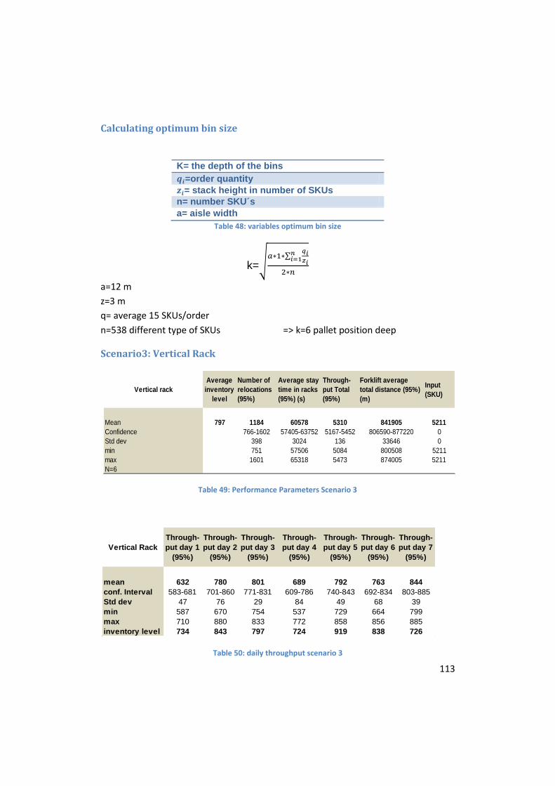
113

Calculating optimum bin size

K= the depth of the bins

=order quantity

= stack height in number of SKUs

n= number SKU´s

a= aisle width

Table 48: variables optimum bin size

k=

a=12 m

z=3 m

q= average 15 SKUs/order

n=538 different type of SKUs => k=6 pallet position deep

Scenario3: Vertical Rack



Vertical rack

Average

inventory

level

Number of

relocations

(95%)

Average stay

time in racks

(95%) (s)

Through-

put Total

(95%)

Forklift average


(m)

Input

(SKU)

Mean 797 1184 60578 5310 841905 5211

Confidence 766-1602 57405-63752 5167-5452 806590-877220 0

Std dev 398 3024 136 33646 0

min 751 57506 5084 800508 5211

max 1601 65318 5473 874005 5211

N=6

Vertical Rack

Through-

put day 1

(95%)

Through-

put day 2

(95%)

Through-

put day 3

(95%)

Through-

put day 4

(95%)

Through-

put day 5

(95%)

Through-

put day 6

(95%)

Through-

put day 7

(95%)

mean 632 780 801 689 792 763 844

conf. Interval 583-681 701-860 771-831 609-786 740-843 692-834 803-885

Std dev 47 76 29 84 49 68 39

min 587 670 754 537 729 664 799

max 710 880 833 772 858 856 885

inventory level 734 843 797 724 919 838 726

114

Scenario 4: 4 truck 4 forklifts


Table 52: Daily Throughput Scenario 4

Scenario 5: Higher Capacity Layout


4 trucks and 4 forklifts

Average

inventory

level

Number of

relocations

(95%)

Average stay

time in racks

(95%) (s)

Through-

put Total

(95%)

Forklift average


(m)

Input

(SKU)

Mean 627 414 36968 5224 856771 5211

Confidence 363-465 35630-38630 5197-5290 847187-866354 0

Std dev 49 1275 44 9130 0

min 348 35445 5186 846980 5211

max 486 38849 5318 869219 5211

N=6

4 trucks, 4

forklifts

Through-

put day 1

(95%)

Through-

put day 2

(95%)

Through-

put day 3

(95%)

Through-

put day 4

(95%)

Through-

put day 5

(95%)

Through-

put day 6

(95%)

Through-

put day 7

(95%)

mean 776 744 690 564 941 714 814

conf. Interval 711-842 704-784 678-702 554-576 927-954 686-743 796-832

Std dev 62 38 12 10 48 27 17

min 669 721 670 554 834 664 797

max 850 820 705 582 973 740 846

inventory level 580 545 535 573 893 663 600

High capacity layoutAverage

Inventory

Level

Number of

relocations

(95%)

Average stay

time in racks

(95%) (s)

Through-

put Total

(95%)

Forklift average


(m)

Input

(SKU)

Mean 786 1311 56221 5220 1435681 5211

Confidence 674-1948 52804-59639 5016-5423 1416742-1454619 0

Std dev 607 3256 194 18043 0

min 732 52424 4951 1410485 5211

max 2071 60257 5456 1466361 5211

N=6

115

Table 54: Daily throughput scenario 5

High capacity

layout

Through-

put day 1

(95%)

Through-

put day 2

(95%)

Through-

put day 3

(95%)

Through-

put day 4

(95%)

Through-

put day 5

(95%)

Through-

put day 6

(95%)

Through-

put day 7

(95%)

mean 622 855 815 626 728 741 833

conf. Interval 541-703 812-898 749-880 536-717 604-852 703-779 784-881

Std dev 77 41 62 86 119 36 46

min 490 805 752 561 578 703 779

max 723 915 879 772 858 797 884

inventory level 727 846 725 638 896 879 789

simulation of finished goods inventory - lund...

Documents