simulation of electromagnetic fields

”Simulation of Electromagnetic Fields”

1

SIMULATION OF

ELECTROMAGNETIC

FIELDS


2

CONTENTS

1. MATLAB FOR BEGINNERS 1.1 Getting Started 1.2 Addition operation in MATLAB 1.3 Subtraction Operation 1.4 Multiplication Operation 1.5 Writing a program in MATLAB 1.6 General programming Commands in MATLAB

2. MATLAB COMMANDS 2.1 quiver3 2.2 vectarrow

2.3 hold 2.4 num2str 2.5 sqrt 2.6 text 2.7.1 xlabel 2.7.2 ylabel 2.7.3 zlabel 2.7.4 title 2.8 patch 2.9 surf

3. Co-Ordinate Systems 3.1 Addition of two vectors using Parallelogram rule 3.2 Addition of two vectors using head to tail rule 3.3 Plotting of unit vectors 3.4 Calculation and representation of unit vector 3.5 Illustration of position vector 3.6 Plotting of position vectors 3.7 Calculation of angle between vectors 3.8 Representation of two planes with ‘x’ constant 3.9 Representation of planes in X-Y and Z co-ordinates 3.10 Representation of differential element in Cartesian co-ordinates 3.11 Representation of surface with φ constant 3.12 Representation of surface with z constant 3.13 Representation of surface with ρ constant 3.14 Representation of surfaces in cylindrical co-ordinates 3.15 Representation of differential elements in cylindrical co-ordinates 3.16 Representation of surface with θ constant 3.17 Representation of surface with r constant 3.18 Representation of surfaces with r, θ and φ constant 3.19 Evaluation of surface and volume integrals of a cylinder

4. MATLAB COMMANDS FOR VISUALIZATION OF ELECTROMAGNETIC FIELDS


3

4.1 Use of meshgrid command

4.2 Use of Peaks Command

4.4 Divergnce

4.5 Contour

4.6 Evaluation of divergence of a vector

4.7 Calculate and plot the divergence of a vector field

4.8 Calculate and plot the gradient of a function

4.9 Plot the gradient of a function

4.10 Plot the curl of a function

5. EXERCISE PROBLEMS


4

1. MATLAB FOR BEGINNERS

1.1 Getting Started

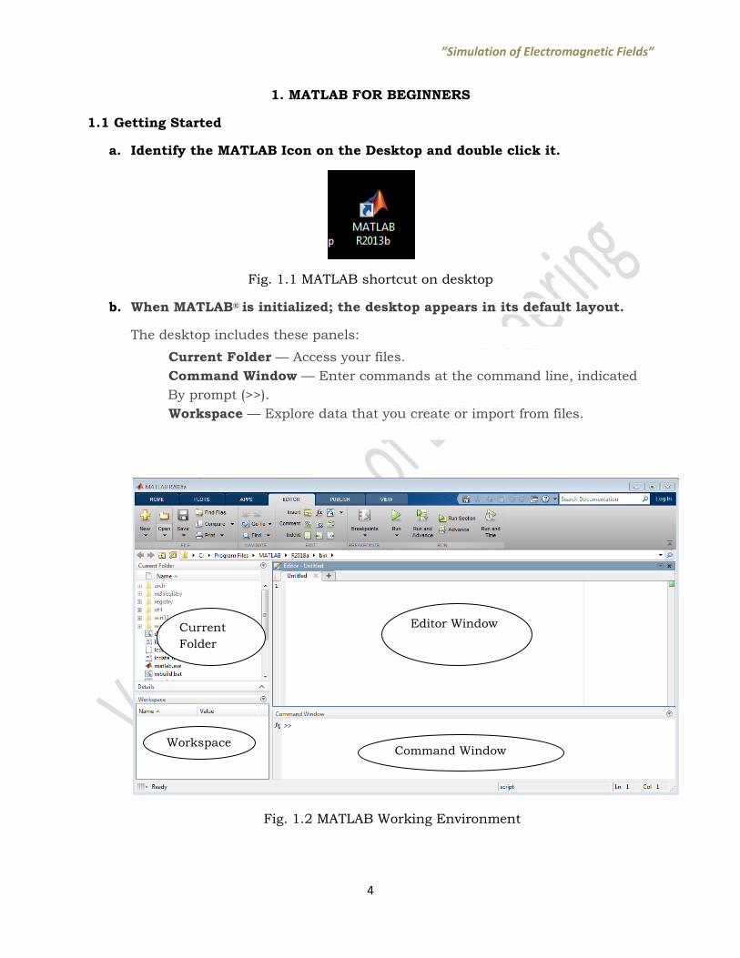
a. Identify the MATLAB Icon on the Desktop and double click it.

Fig. 1.1 MATLAB shortcut on desktop

b. When MATLAB® is initialized; the desktop appears in its default layout.

The desktop includes these panels:

Current Folder — Access your files.

Command Window — Enter commands at the command line, indicated

By prompt (>>).

Workspace — Explore data that you create or import from files.

Fig. 1.2 MATLAB Working Environment

Editor Window

Command Window Workspace

Current

Folder


5

c. Every variable is saved as a matrix and if a variable ‘a’ is entered it is saved in work space as matrix .Its size can be found by using the command size(a).

Fig. 1.3 MATLAB Workspace

d. Columns are separated by commas or by space.

Fig. 1.4 Determining size of a variable in MATLAB

e. Rows are separated by semicolon.


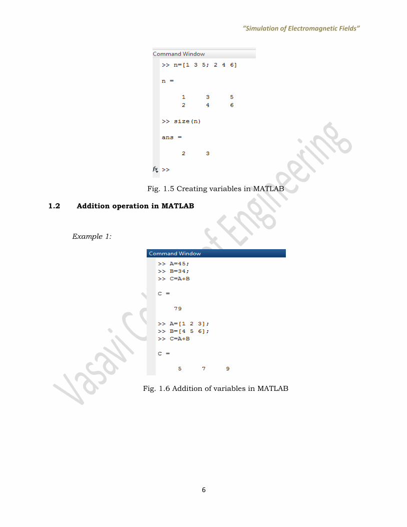
6

Fig. 1.5 Creating variables in MATLAB

1.2 Addition operation in MATLAB

Example 1:

Fig. 1.6 Addition of variables in MATLAB


7

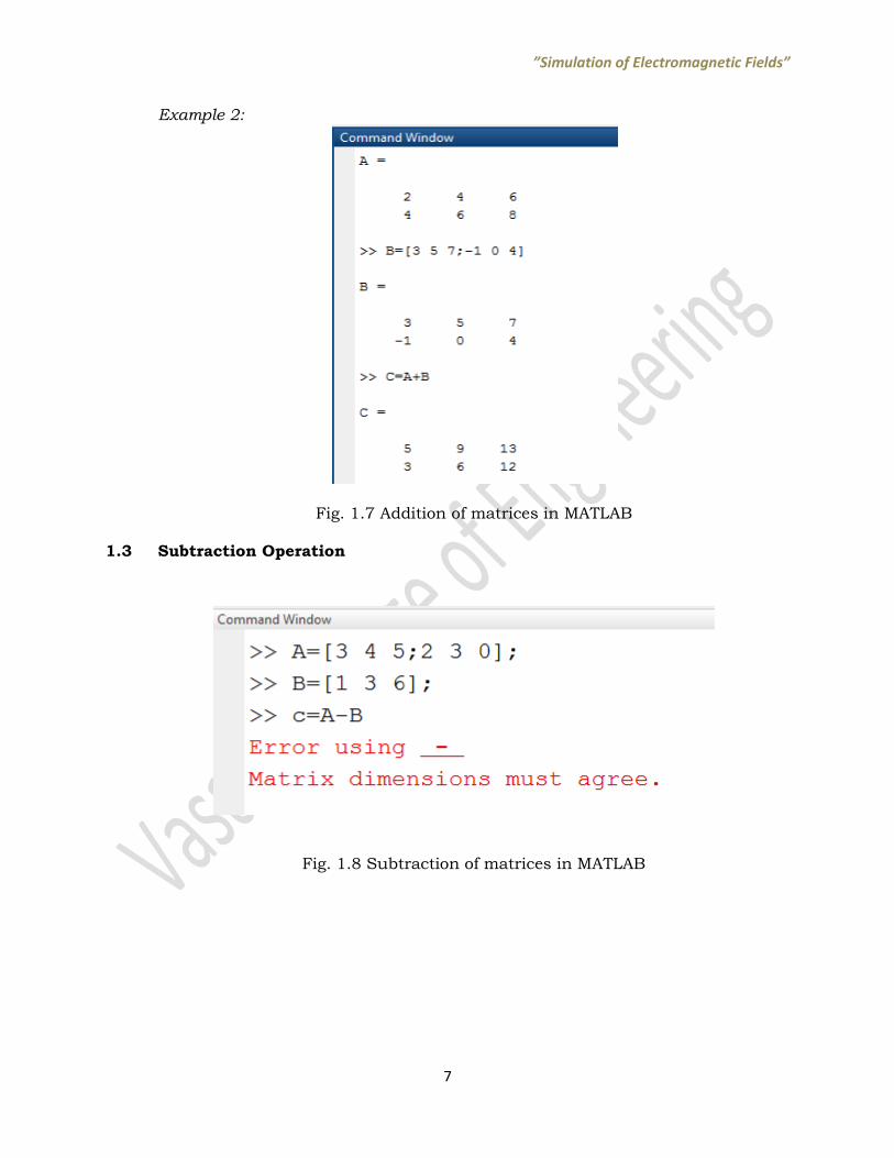
Example 2:

Fig. 1.7 Addition of matrices in MATLAB

1.3 Subtraction Operation

Fig. 1.8 Subtraction of matrices in MATLAB


8

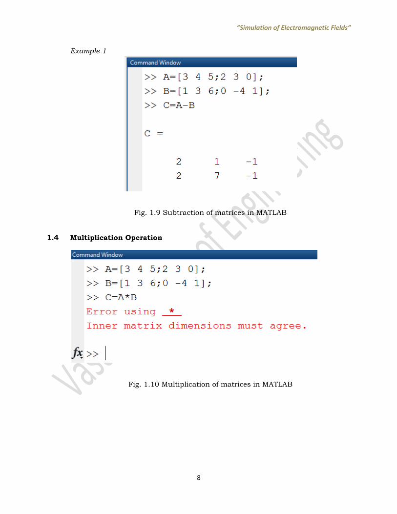
Example 1

Fig. 1.9 Subtraction of matrices in MATLAB

1.4 Multiplication Operation

Fig. 1.10 Multiplication of matrices in MATLAB


9

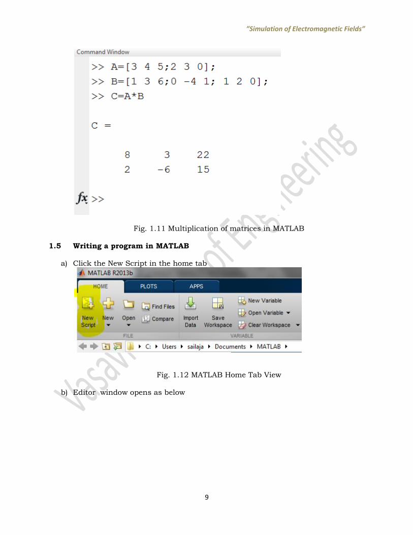
Fig. 1.11 Multiplication of matrices in MATLAB

1.5 Writing a program in MATLAB

a) Click the New Script in the home tab

Fig. 1.12 MATLAB Home Tab View

b) Editor window opens as below


10

Fig. 1.12 MATLAB Editor Window

c) Write the program in this window Example: Program to find the sum of 1 to n numbers

Fig. 1.13 MATLAB program for addition of first ‘n’ numbers clc :clc clears the command window and homes the cursor.


11

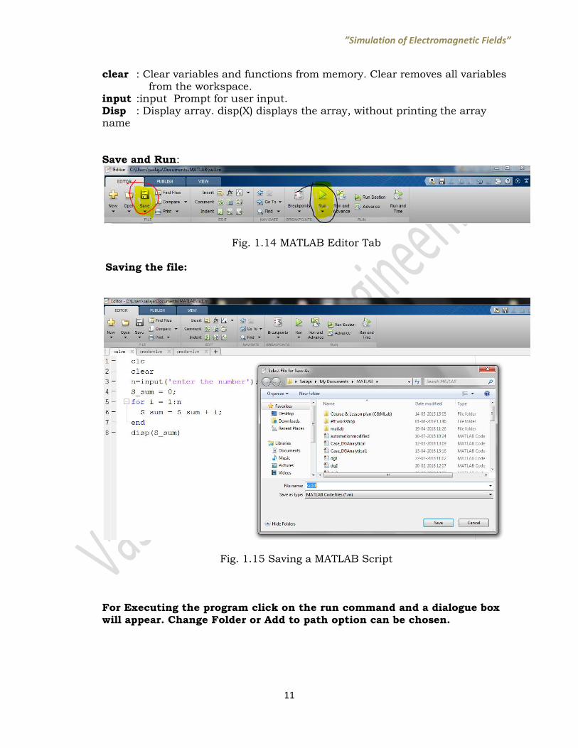
clear : Clear variables and functions from memory. Clear removes all variables from the workspace. input :input Prompt for user input. Disp : Display array. disp(X) displays the array, without printing the array name Save and Run:

Fig. 1.14 MATLAB Editor Tab Saving the file:

Fig. 1.15 Saving a MATLAB Script For Executing the program click on the run command and a dialogue box will appear. Change Folder or Add to path option can be chosen.


12

Fig. 1.16 Executing a MATLAB Script If there are no errors in the program MATLAB waits for the input

Fig. 1.17 Giving input to MATLAB Script After entering input output of the program will be displayed


13

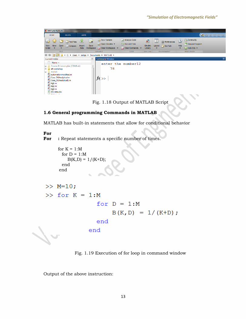
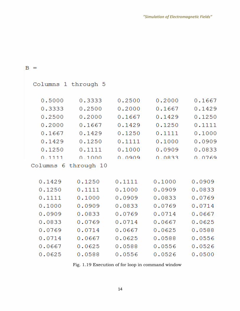
Fig. 1.18 Output of MATLAB Script 1.6 General programming Commands in MATLAB MATLAB has built-in statements that allow for conditional behavior For For : Repeat statements a specific number of times.

for K = 1:M for D = 1:M B(K,D) = 1/(K+D); end end

Fig. 1.19 Execution of for loop in command window Output of the above instruction:


14

Fig. 1.19 Execution of for loop in command window


15

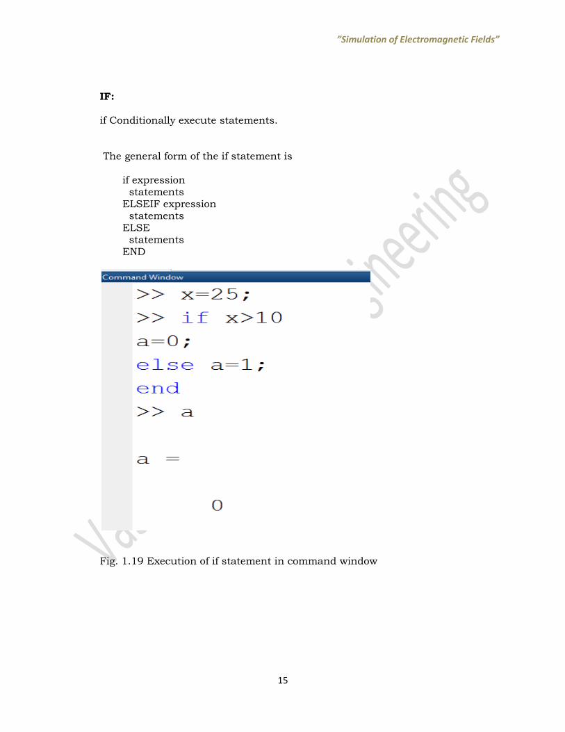
IF: if Conditionally execute statements. The general form of the if statement is if expression statements ELSEIF expression statements ELSE statements END

Fig. 1.19 Execution of if statement in command window


16

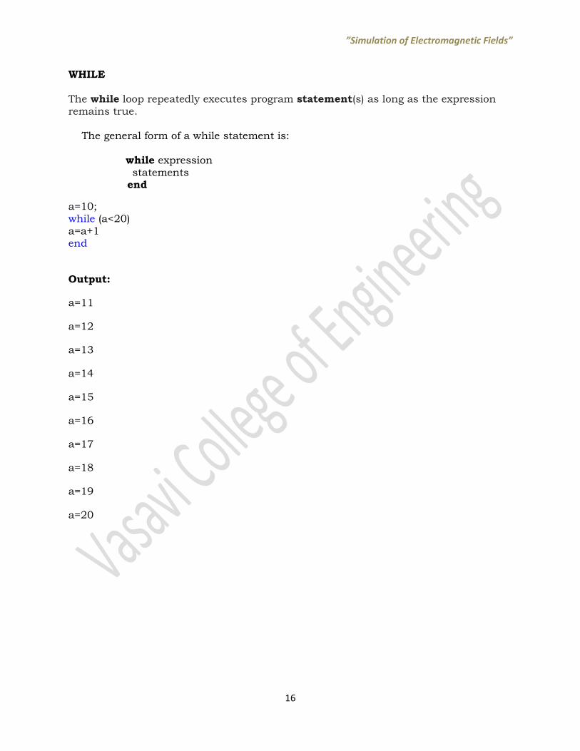
WHILE

The while loop repeatedly executes program statement(s) as long as the expression remains true. The general form of a while statement is:

while expression statements end

a=10; while (a<20) a=a+1 end

Output:

a=11

a=12

a=13

a=14

a=15

a=16

a=17

a=18

a=19

a=20


17

2. MATLAB COMMANDS

2.1 quiver3

quiver3(X,Y,Z,U,V,W,S) plots velocity vectors as arrows with components (u,v,w) at

the points (x,y,z). The matrices X,Y,Z,U,V,W must all be the same size and contain the

corresponding position and velocity components. It automatically scales the arrows to

fit and then stretches them by S. Use S=0 to plot the arrows without the automatic

scaling. [Mathworks Documentation]

Example 2.1:

quiver3([0 0 0],[0 0 0],[0 0 0],[15 0 0],[0 15 0],[0 0 15],0); It plots vectors of length equal to 15 in x,y,z planes from origin.

Fig 2.1 Plot indicating the function of command ‘quiver3’ in a 3d view


18

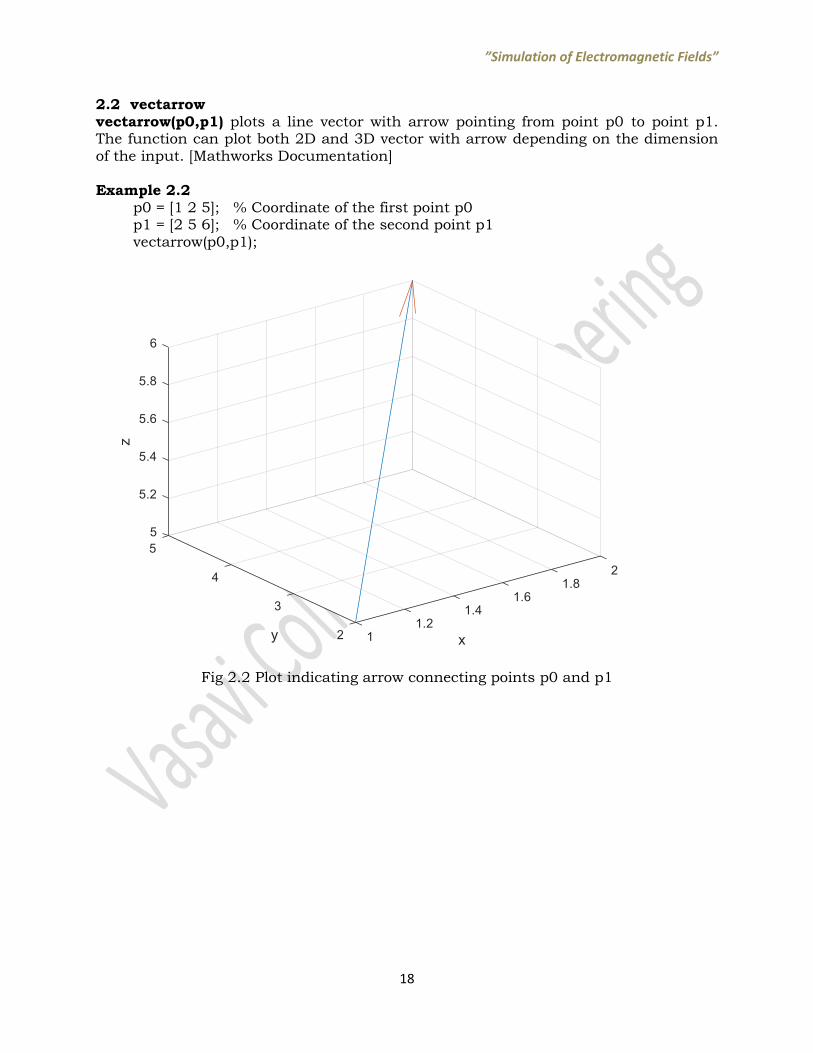
2.2 vectarrow

vectarrow(p0,p1) plots a line vector with arrow pointing from point p0 to point p1. The function can plot both 2D and 3D vector with arrow depending on the dimension of the input. [Mathworks Documentation] Example 2.2 p0 = [1 2 5]; % Coordinate of the first point p0 p1 = [2 5 6]; % Coordinate of the second point p1 vectarrow(p0,p1);

Fig 2.2 Plot indicating arrow connecting points p0 and p1


19

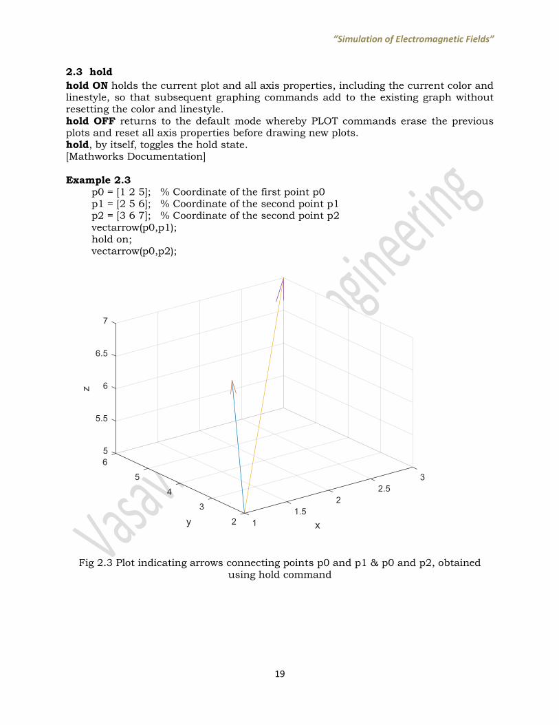
2.3 hold

hold ON holds the current plot and all axis properties, including the current color and linestyle, so that subsequent graphing commands add to the existing graph without resetting the color and linestyle. hold OFF returns to the default mode whereby PLOT commands erase the previous plots and reset all axis properties before drawing new plots. hold, by itself, toggles the hold state. [Mathworks Documentation] Example 2.3 p0 = [1 2 5]; % Coordinate of the first point p0 p1 = [2 5 6]; % Coordinate of the second point p1 p2 = [3 6 7]; % Coordinate of the second point p2

vectarrow(p0,p1); hold on; vectarrow(p0,p2);

Fig 2.3 Plot indicating arrows connecting points p0 and p1 & p0 and p2, obtained using hold command


20

2.4 num2str

num2str Convert numbers to character representation T = num2str(X) converts the matrix X into its character representation T with about 4 digits and an exponent if required. This is useful for labeling plots with the TITLE, XLABEL, YLABEL, and TEXT commands. [Mathworks Documentation] Example 2.4 p0 = [1 2 5];

p1 = [2 5 6]; p2 = [3 6 7];

A=num2str(p0)

B=num2str(p1)

C=num2str(p2)

Output A = '1 2 5' B = '2 5 6' C = '3 6 7' 2.5. sqrt sqrt(X) is the square root of the elements of X. Complex results are produced if X is not positive. [Mathworks Documentation] Example 2.5.1 A=sqrt(30)

Output

A = 5.4772

Example 2.5.2 B=sqrt(-1)

Output

B= 0.0000 + 1.0000i


21

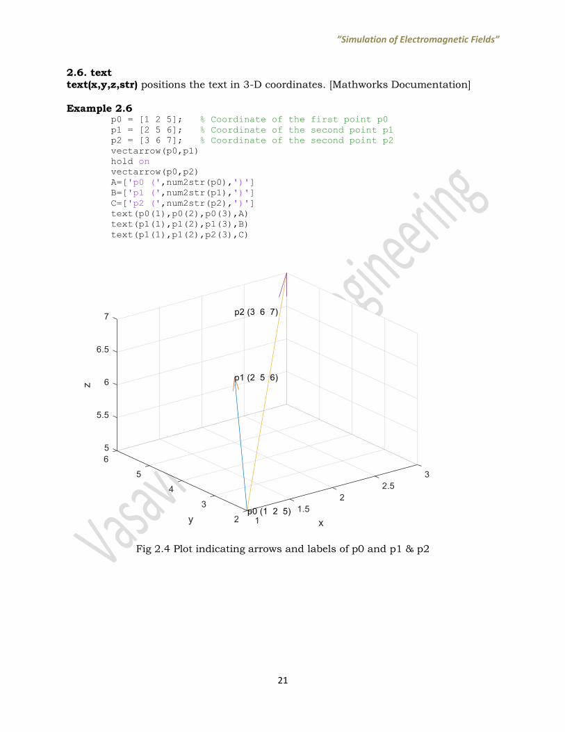
2.6. text

text(x,y,z,str) positions the text in 3-D coordinates. [Mathworks Documentation] Example 2.6 p0 = [1 2 5]; % Coordinate of the first point p0 p1 = [2 5 6]; % Coordinate of the second point p1 p2 = [3 6 7]; % Coordinate of the second point p2 vectarrow(p0,p1) hold on vectarrow(p0,p2) A=['p0 (',num2str(p0),')'] B=['p1 (',num2str(p1),')'] C=['p2 (',num2str(p2),')'] text(p0(1),p0(2),p0(3),A) text(p1(1),p1(2),p1(3),B) text(p1(1),p1(2),p2(3),C)

Fig 2.4 Plot indicating arrows and labels of p0 and p1 & p2


22

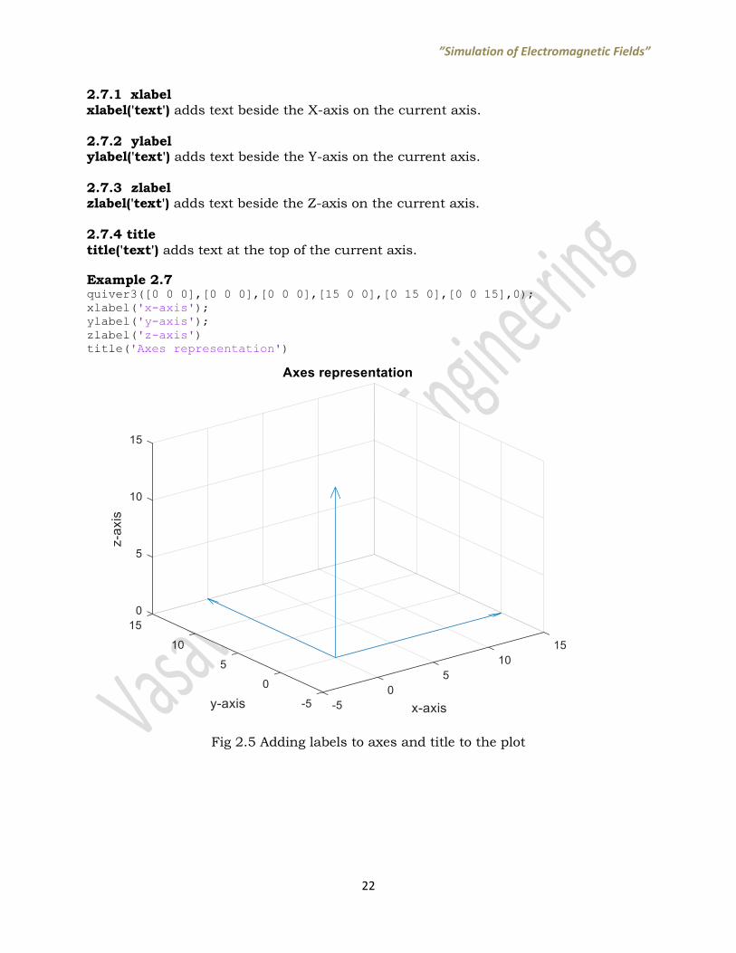
2.7.1 xlabel

xlabel('text') adds text beside the X-axis on the current axis. 2.7.2 ylabel ylabel('text') adds text beside the Y-axis on the current axis. 2.7.3 zlabel zlabel('text') adds text beside the Z-axis on the current axis. 2.7.4 title

title('text') adds text at the top of the current axis.

Example 2.7 quiver3([0 0 0],[0 0 0],[0 0 0],[15 0 0],[0 15 0],[0 0 15],0); xlabel('x-axis'); ylabel('y-axis'); zlabel('z-axis') title('Axes representation')

Fig 2.5 Adding labels to axes and title to the plot


23

2.8 patch

patch(X,Y,Z,C) creates the polygons in 3-D coordinates using X, Y, and Z. To view the polygons in a 3-D view, use the view(3) command. C determines the polygon colors. Example 2.8 quiver3([0 0 0],[0 0 0],[0 0 0],[25 0 0],[0 25 0],[0 0 25]); hold on; quiver3([0 0 0],[0 0 0],[0 0 0],[-25 0 0],[0 -25 0],[0 0 -25]); hold on; x=6; y1=-15;y2=15;y3=15;y4=-15; z1=-15;z2=-15;z3=15;z4=15; patch([x x x x x], [y1 y2 y3 y4 y1], [z1 z2 z3 z4 z1],'green'); A=[x y1 z1];B=[x y2 z2];C=[x y3 z3];D=[x y4 z4]; Astr=['A (',num2str(A),')'];Bstr=['B (',num2str(B),')']; Cstr=['C (',num2str(C),')'];Dstr=['D (',num2str(D),')']; text(A(1),A(2),A(3),Astr);text(B(1),B(2),B(3),Bstr); text(C(1),C(2),C(3),Cstr);text(D(1),D(2),D(3),Dstr); xlabel('x-axis');ylabel('y-axis');zlabel('z-axis'); title('Patch command-polygon');

Fig 2.6 Plotting a rectangle using patch command


24

2.9 surf

surf(X,Y,Z,C) plots the colored parametric surface defined by four matrix arguments. The view point is specified by VIEW. The axis labels are determined by the range of X, Y and Z, or by the current setting of AXIS. The color scaling is determined by the range of C, or by the current setting of CAXIS. The scaled color values are used as indices into the current COLORMAP. surf(x,y,Z) and surf(x,y,Z,C), with two vector arguments replacing the first two matrix arguments, must have length(x) = n and length(y) = m where [m,n] = size(Z). In this case, the vertices of the surface patches are the triples (x(j), y(i), Z(i,j)). Note that x corresponds to the columns of Z and y corresponds to the rows. Example 2.9 quiver3([0 0 0],[0 0 0],[0 0 0],[25 0 0],[0 25 0],[0 0 25]) hold on quiver3([0 0 0],[0 0 0],[0 0 0],[-25 0 0],[0 -25 0],[0 0 -25]) hold on theta=0:pi/10:2*pi; r=10; x1=r*cos(theta); y1=r*sin(theta); for k=1:length(x1) z1(k)=-5; z2(k)=5; end x=[x1;x1]; y=[y1;y1]; z=[z1;z2]; surf(x,y,z); xlabel('x-axis');ylabel('y-axis');zlabel('z-axis');

Fig 2.7 Plotting a cylinder using surf command


25

3.MATLAB PROGRAMS

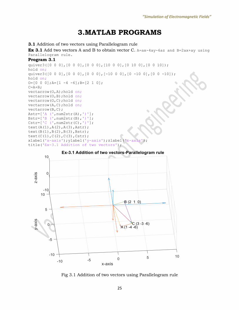
3.1 Addition of two vectors using Parallelogram rule

Ex 3.1 Add two vectors A and B to obtain vector C. A=ax-4ay-6az and B=2ax+ay using Parallelogram rule.

Program 3.1

quiver3([0 0 0],[0 0 0],[0 0 0],[10 0 0],[0 10 0],[0 0 10]);

hold on;

quiver3([0 0 0],[0 0 0],[0 0 0],[-10 0 0],[0 -10 0],[0 0 -10]);

hold on;

O=[0 0 0];A=[1 -4 -6];B=[2 1 0];

C=A+B;

vectarrow(O,A);hold on;

vectarrow(O,B);hold on;

vectarrow(O,C);hold on;

vectarrow(A,C);hold on;

vectarrow(B,C);

Astr=['A (',num2str(A),')'];

Bstr=['B (',num2str(B),')'];

Cstr=['C (',num2str(C),')'];

text(A(1),A(2),A(3),Astr);

text(B(1),B(2),B(3),Bstr);

text(C(1),C(2),C(3),Cstr);

xlabel('x-axis');ylabel('y-axis');zlabel('z-axis');

title('Ex-3.1 Addition of two vectors');

Fig 3.1 Addition of two vectors using Parallelogram rule


26

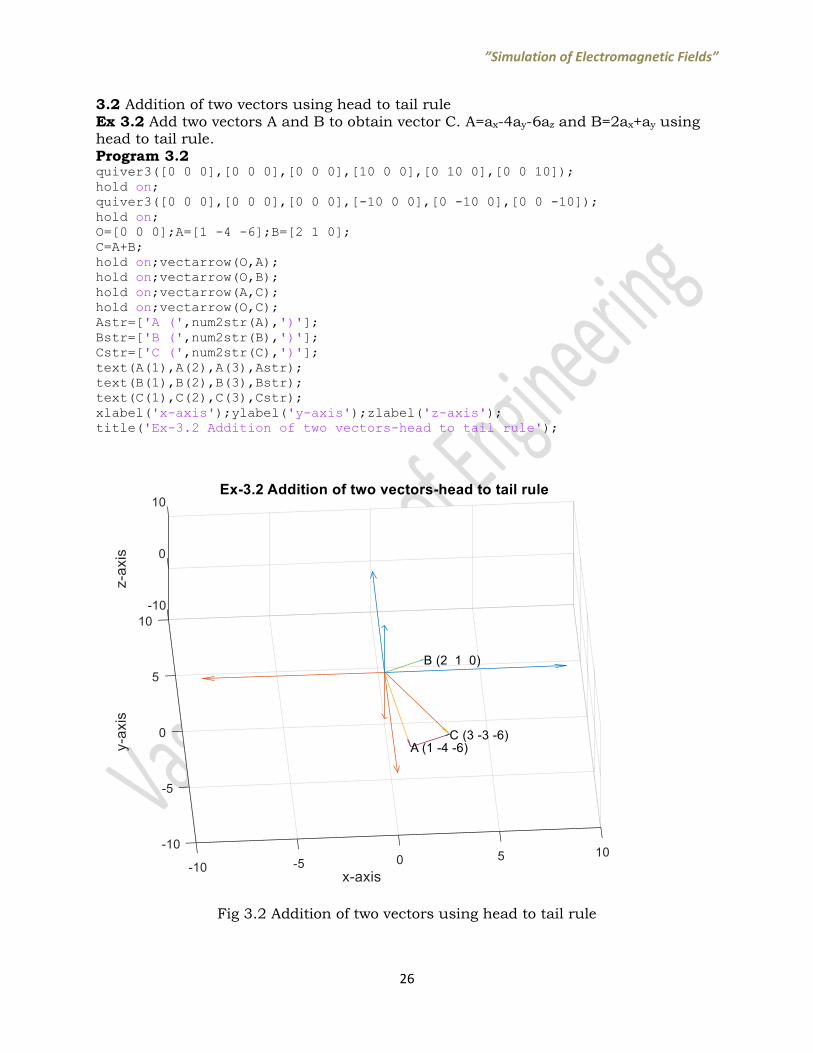
3.2 Addition of two vectors using head to tail rule

Ex 3.2 Add two vectors A and B to obtain vector C. A=ax-4ay-6az and B=2ax+ay using head to tail rule. Program 3.2 quiver3([0 0 0],[0 0 0],[0 0 0],[10 0 0],[0 10 0],[0 0 10]); hold on; quiver3([0 0 0],[0 0 0],[0 0 0],[-10 0 0],[0 -10 0],[0 0 -10]); hold on; O=[0 0 0];A=[1 -4 -6];B=[2 1 0]; C=A+B; hold on;vectarrow(O,A); hold on;vectarrow(O,B); hold on;vectarrow(A,C); hold on;vectarrow(O,C); Astr=['A (',num2str(A),')']; Bstr=['B (',num2str(B),')']; Cstr=['C (',num2str(C),')']; text(A(1),A(2),A(3),Astr); text(B(1),B(2),B(3),Bstr); text(C(1),C(2),C(3),Cstr); xlabel('x-axis');ylabel('y-axis');zlabel('z-axis'); title('Ex-3.2 Addition of two vectors-head to tail rule');

Fig 3.2 Addition of two vectors using head to tail rule


27

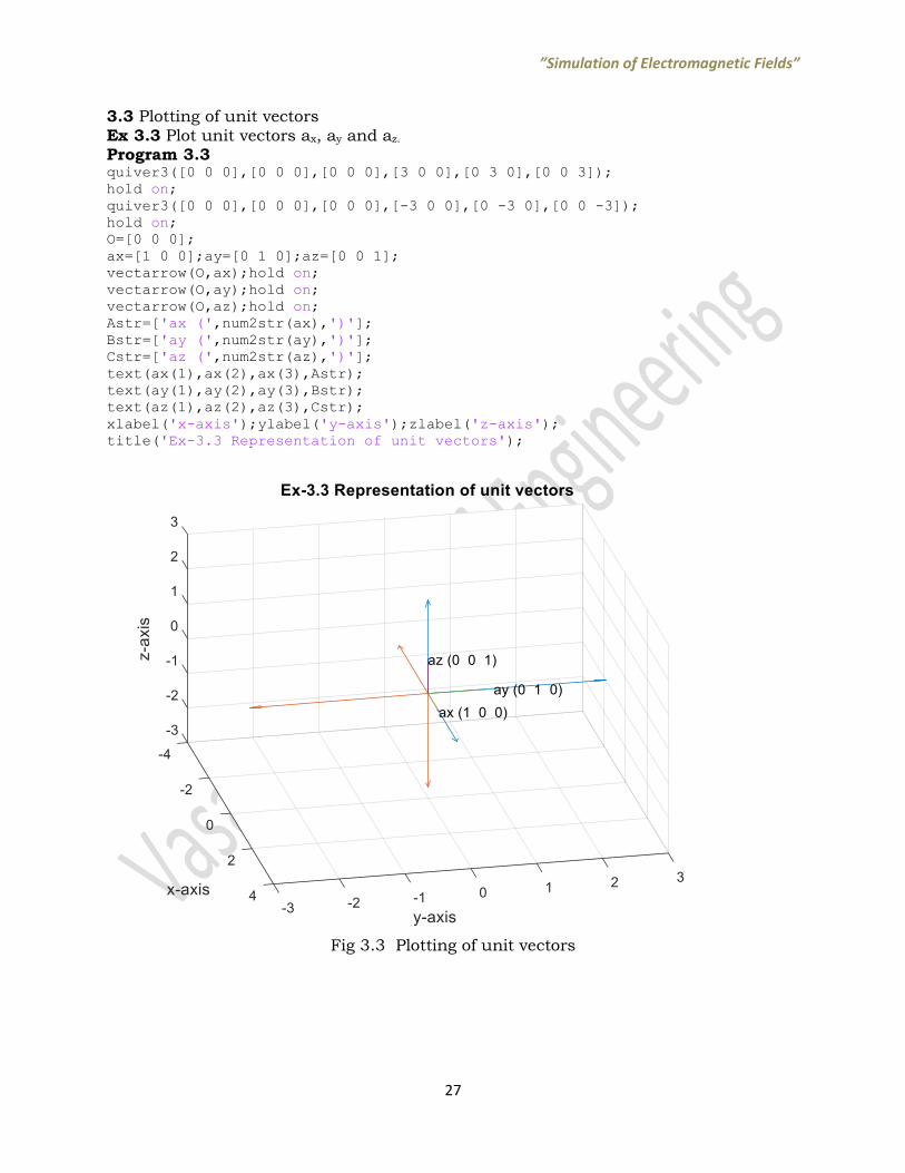
3.3 Plotting of unit vectors Ex 3.3 Plot unit vectors ax, ay and az. Program 3.3 quiver3([0 0 0],[0 0 0],[0 0 0],[3 0 0],[0 3 0],[0 0 3]); hold on; quiver3([0 0 0],[0 0 0],[0 0 0],[-3 0 0],[0 -3 0],[0 0 -3]); hold on; O=[0 0 0]; ax=[1 0 0];ay=[0 1 0];az=[0 0 1]; vectarrow(O,ax);hold on; vectarrow(O,ay);hold on; vectarrow(O,az);hold on; Astr=['ax (',num2str(ax),')']; Bstr=['ay (',num2str(ay),')']; Cstr=['az (',num2str(az),')']; text(ax(1),ax(2),ax(3),Astr); text(ay(1),ay(2),ay(3),Bstr); text(az(1),az(2),az(3),Cstr); xlabel('x-axis');ylabel('y-axis');zlabel('z-axis'); title('Ex-3.3 Representation of unit vectors');

Fig 3.3 Plotting of unit vectors


28

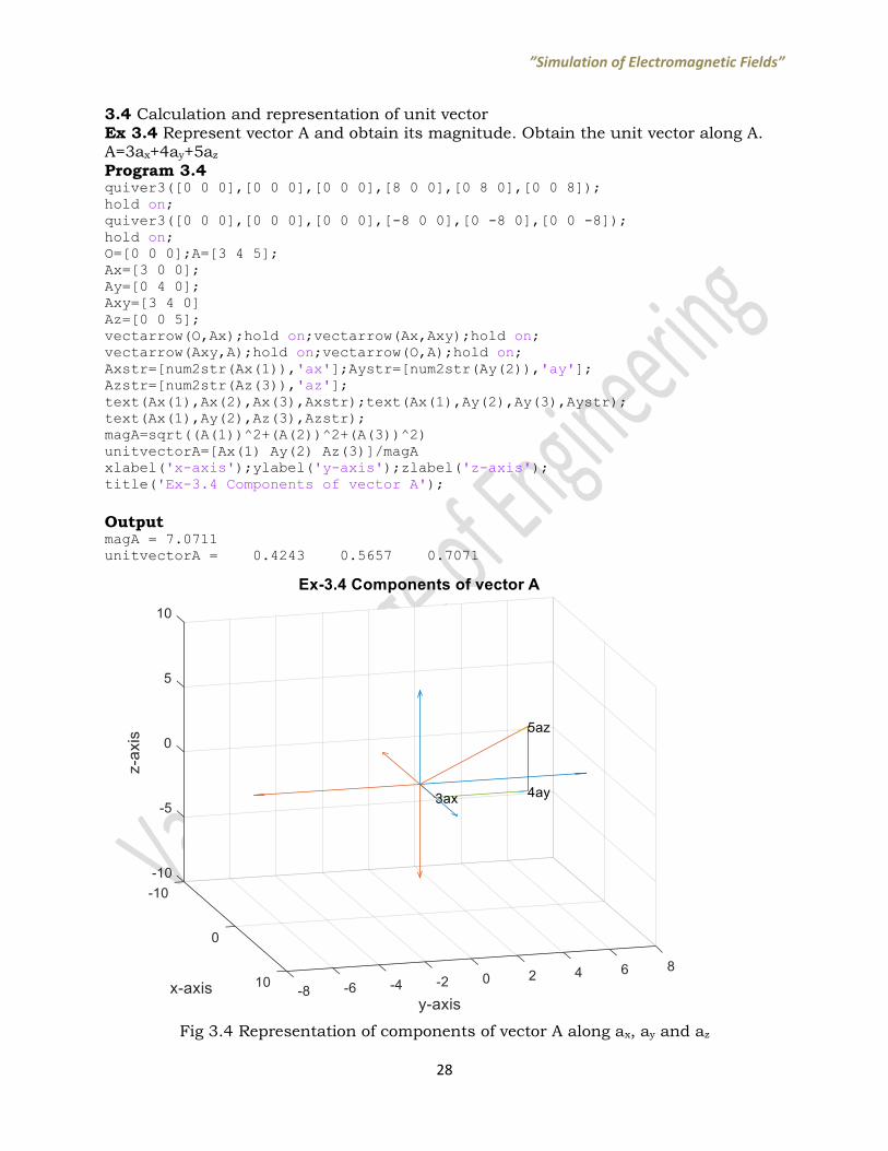
3.4 Calculation and representation of unit vector Ex 3.4 Represent vector A and obtain its magnitude. Obtain the unit vector along A. A=3ax+4ay+5az Program 3.4 quiver3([0 0 0],[0 0 0],[0 0 0],[8 0 0],[0 8 0],[0 0 8]); hold on; quiver3([0 0 0],[0 0 0],[0 0 0],[-8 0 0],[0 -8 0],[0 0 -8]); hold on; O=[0 0 0];A=[3 4 5]; Ax=[3 0 0]; Ay=[0 4 0]; Axy=[3 4 0] Az=[0 0 5]; vectarrow(O,Ax);hold on;vectarrow(Ax,Axy);hold on; vectarrow(Axy,A);hold on;vectarrow(O,A);hold on; Axstr=[num2str(Ax(1)),'ax'];Aystr=[num2str(Ay(2)),'ay']; Azstr=[num2str(Az(3)),'az']; text(Ax(1),Ax(2),Ax(3),Axstr);text(Ax(1),Ay(2),Ay(3),Aystr); text(Ax(1),Ay(2),Az(3),Azstr); magA=sqrt((A(1))^2+(A(2))^2+(A(3))^2) unitvectorA=[Ax(1) Ay(2) Az(3)]/magA xlabel('x-axis');ylabel('y-axis');zlabel('z-axis'); title('Ex-3.4 Components of vector A');

Output magA = 7.0711

unitvectorA = 0.4243 0.5657 0.7071

Fig 3.4 Representation of components of vector A along ax, ay and az


29

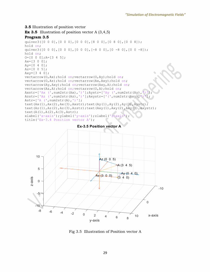
3.5 Illustration of position vector

Ex 3.5 Illustration of position vector A (3,4,5)

Program 3.5

quiver3([0 0 0],[0 0 0],[0 0 0],[8 0 0],[0 8 0],[0 0 8]); hold on; quiver3([0 0 0],[0 0 0],[0 0 0],[-8 0 0],[0 -8 0],[0 0 -8]); hold on; O=[0 0 0];A=[3 4 5]; Ax=[3 0 0]; Ay=[0 4 0]; Az=[0 0 5]; Axy=[3 4 0]; vectarrow(O,Ax);hold on;vectarrow(O,Ay);hold on; vectarrow(O,Az);hold on;vectarrow(Ax,Axy);hold on; vectarrow(Ay,Axy);hold on;vectarrow(Axy,A);hold on; vectarrow(Az,A);hold on;vectarrow(O,A);hold on; Axstr=['Ax (',num2str(Ax),')'];Aystr=['Ay (',num2str(Ay),')']; Azstr=['Az (',num2str(Az),')'];Axystr=['(',num2str(Axy),')']; Astr=['A (',num2str(A),')']; text(Ax(1),Ax(2),Ax(3),Axstr);text(Ay(1),Ay(2),Ay(3),Aystr); text(Az(1),Az(2),Az(3),Azstr);text(Axy(1),Axy(2),Axy(3),Axystr); text(A(1),A(2),A(3),Astr); xlabel('x-axis');ylabel('y-axis');zlabel('z-axis'); title('Ex-3.4 Position vector A');

Fig 3.5 Illustration of Position vector A


30

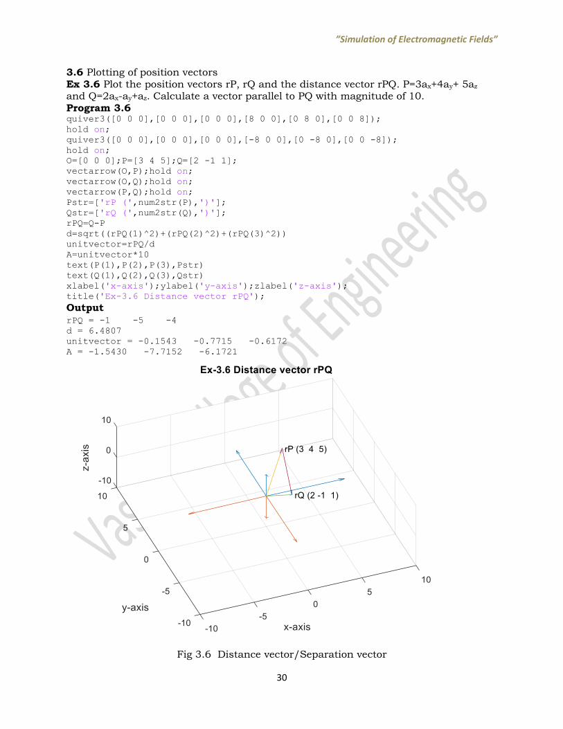
3.6 Plotting of position vectors Ex 3.6 Plot the position vectors rP, rQ and the distance vector rPQ. P=3ax+4ay+ 5az and Q=2ax-ay+az. Calculate a vector parallel to PQ with magnitude of 10. Program 3.6 quiver3([0 0 0],[0 0 0],[0 0 0],[8 0 0],[0 8 0],[0 0 8]); hold on; quiver3([0 0 0],[0 0 0],[0 0 0],[-8 0 0],[0 -8 0],[0 0 -8]); hold on; O=[0 0 0];P=[3 4 5];Q=[2 -1 1]; vectarrow(O,P);hold on; vectarrow(O,Q);hold on; vectarrow(P,Q);hold on; Pstr=['rP (',num2str(P),')']; Qstr=['rQ (',num2str(Q),')']; rPQ=Q-P

d=sqrt((rPQ(1)^2)+(rPQ(2)^2)+(rPQ(3)^2))

unitvector=rPQ/d A=unitvector*10 text(P(1),P(2),P(3),Pstr) text(Q(1),Q(2),Q(3),Qstr) xlabel('x-axis');ylabel('y-axis');zlabel('z-axis'); title('Ex-3.6 Distance vector rPQ');

Output rPQ = -1 -5 -4

d = 6.4807

unitvector = -0.1543 -0.7715 -0.6172

A = -1.5430 -7.7152 -6.1721

Fig 3.6 Distance vector/Separation vector


31

3.7 Calculation of angle between vectors Ex 3.7 Given vectors A=3ax+4ay+az and B=2ay-5az, find the angle between A and B Program 3.7 A=[3 4 1]; B=[0 2 -5]; crossAB=cross(A,B) magcrossAB=sqrt((crossAB(1))^2+(crossAB(2))^2+(crossAB(3))^2) dotAB=dot(A,B) magA=sqrt((A(1))^2+(A(2))^2+(A(3))^2) magB=sqrt((B(1))^2+(B(2))^2+(B(3))^2) costhetaAB=dotAB/(magA*magB) thetaAB1=(acos(costhetaAB))*180/pi sinthetaAB=magcrossAB/(magA*magB) thetaAB2=(asin(sinthetaAB))*180/pi

Output crossAB = -22 15 6

magcrossAB = 27.2947

dotAB = 3

magA = 5.0990

magB = 5.3852

costhetaAB = 0.1093

thetaAB1 = 83.7277

sinthetaAB = 0.9940

thetaAB2 = 83.7277


32

3.8 Representation of two planes with ‘x’ constant

Ex 3.8 Draw two planes with x=constant

Program 3.8

quiver3([0 0 0],[0 0 0],[0 0 0],[25 0 0],[0 25 0],[0 0 25]) hold on quiver3([0 0 0],[0 0 0],[0 0 0],[-25 0 0],[0 -25 0],[0 0 -25]) hold on x=10; y1=-15;y2=15;y3=15;y4=-15; z1=-15;z2=-15;z3=15;z4=15; patch([x x x x x], [y1 y2 y3 y4 y1], [z1 z2 z3 z4 z1],'green'); G1=[x y1 z1];G2=[x y2 z2];G3=[x y3 z3];G4=[x y4 z4]; g1=['g1 (',num2str(G1),')'];g2=['g2 (',num2str(G2),')']; g3=['g3 (',num2str(G3),')'];g4=['g4 (',num2str(G4),')']; text(x,y1,z1,g1);text(x,y2,z2,g2);text(x,y3,z3,g3);text(x,y4,z4,g4); hold on x=-10; patch([x x x x x], [y1 y2 y3 y4 y1], [z1 z2 z3 z4 z1],'red'); R1=[x y1 z1];R2=[x y2 z2];R3=[x y3 z3];R4=[x y4 z4]; r1=['r1 (',num2str(R1),')'];r2=['r2 (',num2str(R2),')']; r3=['r3 (',num2str(R3),')'];r4=['r4 (',num2str(R4),')']; text(x,y1,z1,r1);text(x,y2,z2,r2);text(x,y3,z3,r3);text(x,y4,z4,r4);

xlabel('x-axis');ylabel('y-axis');zlabel('z-axis'); title('Ex-3.8 x-constant planes');

Fig 3.8 Two planes with x=constant


33

3.9 Representation of planes in X-Y and Z co-ordinates Ex 3.9 Draw planes in X-Y and Z axes Program 3.9 quiver3([0 0 0],[0 0 0],[0 0 0],[25 0 0],[0 25 0],[0 0 25]) hold on quiver3([0 0 0],[0 0 0],[0 0 0],[-25 0 0],[0 -25 0],[0 0 -25]) hold on x=6; y1=-13;y2=13;y3=13;y4=-13; z1=-13;z2=-13;z3=13;z4=13; patch([x x x x x], [y1 y2 y3 y4 y1], [z1 z2 z3 z4 z1],'blue') hold on y=8; x1=-13;x2=13;x3=13;x4=-13; z1=-15;z2=-15;z3=15;z4=15; hold on patch([x1 x2 x3 x4 x1], [y y y y y], [z1 z2 z3 z4 z1],'green') z=3; x1=-13;x2=13;x3=13;x4=-13; y1=-15;y2=-15;y3=15;y4=15; hold on patch([x1 x2 x3 x4 x1], [y1 y2 y3 y4 y1], [z z z z z],'red') xlabel('x-axis');ylabel('y-axis');zlabel('z-axis'); title('Ex-3.9-X,Y and Z planes ');

Fig 3.9 X-Y and Z planes


34

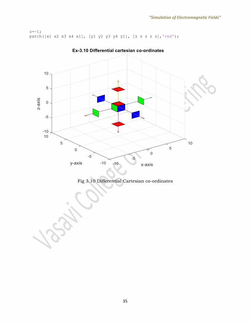
3.10 Representation of differential element in Cartesian co-ordinates

Ex 3.10 Draw a differential element in Cartesian co-ordinates

Program 3.10

clear all quiver3([0 0 0],[0 0 0],[0 0 0],[10 0 0],[0 10 0],[0 0 10]); hold on; quiver3([0 0 0],[0 0 0],[0 0 0],[-10 0 0],[0 -10 0],[0 0 -10]); hold on; xlabel('x-axis');ylabel('y-axis');zlabel('z-axis'); title('Ex-3.10 Differential cartesian co-ordinates'); x=6; y1=-1;y2=1;y3=1;y4=-1 z1=-1;z2=-1;z3=1;z4=1 patch([x x x x x], [y1 y2 y3 y4 y1], [z1 z2 z3 z4 z1],'green'); hold on; x=-6; patch([x x x x x], [y1 y2 y3 y4 y1], [z1 z2 z3 z4 z1],'green'); y=6; x1=-1;x2=1;x3=1;x4=-1; z1=-1;z2=-1;z3=1;z4=1; hold on; patch([x1 x2 x3 x4 x1], [y y y y y], [z1 z2 z3 z4 z1],'blue'); hold on; y=-6; patch([x1 x2 x3 x4 x1], [y y y y y], [z1 z2 z3 z4 z1],'blue'); z=6; x1=-1;x2=1;x3=1;x4=-1; y1=-1;y2=-1;y3=1;y4=1; hold on; patch([x1 x2 x3 x4 x1], [y1 y2 y3 y4 y1], [z z z z z],'red'); hold on; z=-6; patch([x1 x2 x3 x4 x1], [y1 y2 y3 y4 y1], [z z z z z],'red');

x=1; y1=-1;y2=1;y3=1;y4=-1; z1=-1;z2=-1;z3=1; z4=1; patch([x x x x x], [y1 y2 y3 y4 y1], [z1 z2 z3 z4 z1],'green'); hold on; x=-1; patch([x x x x x], [y1 y2 y3 y4 y1], [z1 z2 z3 z4 z1],'green'); y=1; x1=-1;x2=1;x3=1;x4=-1; z1=-1;z2=-1;z3=1;z4=1; hold on; patch([x1 x2 x3 x4 x1], [y y y y y], [z1 z2 z3 z4 z1],'blue'); hold on; y=-1; patch([x1 x2 x3 x4 x1], [y y y y y], [z1 z2 z3 z4 z1],'blue'); z=1; x1=-1;x2=1;x3=1;x4=-1; y1=-1;y2=-1;y3=1;y4=1; hold on; patch([x1 x2 x3 x4 x1], [y1 y2 y3 y4 y1], [z z z z z],'red'); hold on;


35

z=-1; patch([x1 x2 x3 x4 x1], [y1 y2 y3 y4 y1], [z z z z z],'red');

Fig 3.10 Differential Cartesian co-ordinates


36

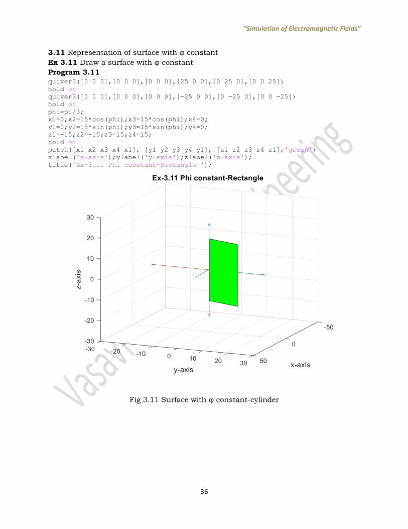
3.11 Representation of surface with φ constant

Ex 3.11 Draw a surface with φ constant

Program 3.11

quiver3([0 0 0],[0 0 0],[0 0 0],[25 0 0],[0 25 0],[0 0 25]) hold on quiver3([0 0 0],[0 0 0],[0 0 0],[-25 0 0],[0 -25 0],[0 0 -25]) hold on phi=pi/3; x1=0;x2=15*cos(phi);x3=15*cos(phi);x4=0; y1=0;y2=15*sin(phi);y3=15*sin(phi);y4=0; z1=-15;z2=-15;z3=15;z4=15; hold on patch([x1 x2 x3 x4 x1], [y1 y2 y3 y4 y1], [z1 z2 z3 z4 z1],'green') xlabel('x-axis');ylabel('y-axis');zlabel('z-axis'); title('Ex-3.11 Phi constant-Rectangle ');

Fig 3.11 Surface with φ constant-cylinder


37

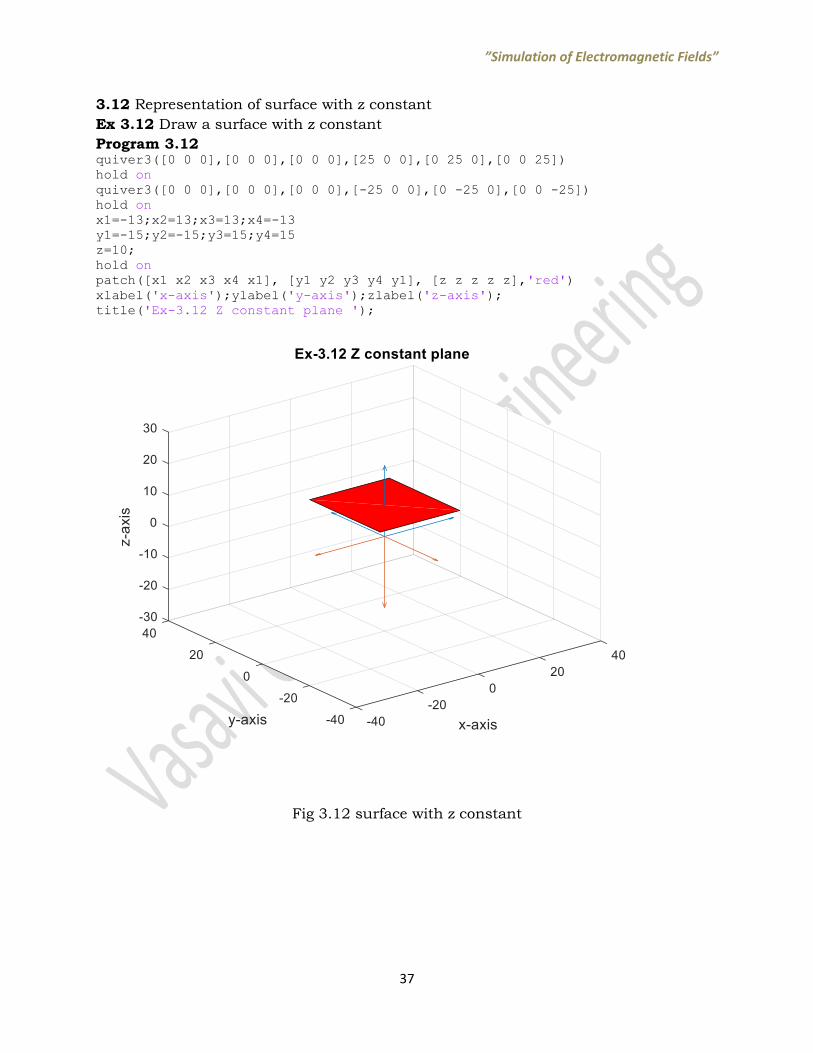
3.12 Representation of surface with z constant

Ex 3.12 Draw a surface with z constant

Program 3.12 quiver3([0 0 0],[0 0 0],[0 0 0],[25 0 0],[0 25 0],[0 0 25]) hold on quiver3([0 0 0],[0 0 0],[0 0 0],[-25 0 0],[0 -25 0],[0 0 -25]) hold on x1=-13;x2=13;x3=13;x4=-13 y1=-15;y2=-15;y3=15;y4=15 z=10; hold on patch([x1 x2 x3 x4 x1], [y1 y2 y3 y4 y1], [z z z z z],'red') xlabel('x-axis');ylabel('y-axis');zlabel('z-axis'); title('Ex-3.12 Z constant plane ');

Fig 3.12 surface with z constant


38

3.13 Representation of surface with ρ constant

Ex 3.13 Draw a surface with ρ constant

Program 3.13

quiver3([0 0 0],[0 0 0],[0 0 0],[25 0 0],[0 25 0],[0 0 25]) hold on quiver3([0 0 0],[0 0 0],[0 0 0],[-25 0 0],[0 -25 0],[0 0 -25]) hold on theta=0:pi/40:2*pi; r=10; x1=r*cos(theta); y1=r*sin(theta); for k=1:length(x1) z1(k)=-15; z2(k)=15; end x=[x1;x1]; y=[y1;y1]; z=[z1;z2]; surf(x,y,z); xlabel('x-axis');ylabel('y-axis');zlabel('z-axis'); title('Ex-3.13 Rho constant-Cylinder ');

Fig 3.13 Surface with ρ constant-cylinder


39

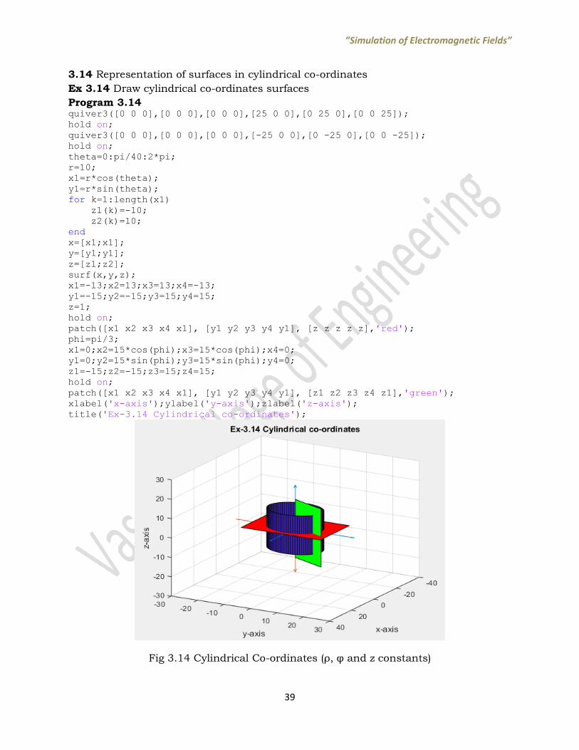
3.14 Representation of surfaces in cylindrical co-ordinates

Ex 3.14 Draw cylindrical co-ordinates surfaces

Program 3.14 quiver3([0 0 0],[0 0 0],[0 0 0],[25 0 0],[0 25 0],[0 0 25]); hold on; quiver3([0 0 0],[0 0 0],[0 0 0],[-25 0 0],[0 -25 0],[0 0 -25]); hold on; theta=0:pi/40:2*pi; r=10; x1=r*cos(theta); y1=r*sin(theta); for k=1:length(x1) z1(k)=-10; z2(k)=10; end x=[x1;x1]; y=[y1;y1]; z=[z1;z2]; surf(x,y,z); x1=-13;x2=13;x3=13;x4=-13; y1=-15;y2=-15;y3=15;y4=15; z=1; hold on; patch([x1 x2 x3 x4 x1], [y1 y2 y3 y4 y1], [z z z z z],'red'); phi=pi/3; x1=0;x2=15*cos(phi);x3=15*cos(phi);x4=0; y1=0;y2=15*sin(phi);y3=15*sin(phi);y4=0; z1=-15;z2=-15;z3=15;z4=15; hold on; patch([x1 x2 x3 x4 x1], [y1 y2 y3 y4 y1], [z1 z2 z3 z4 z1],'green'); xlabel('x-axis');ylabel('y-axis');zlabel('z-axis'); title('Ex-3.14 Cylindrical co-ordinates');

Fig 3.14 Cylindrical Co-ordinates (ρ, φ and z constants)


40

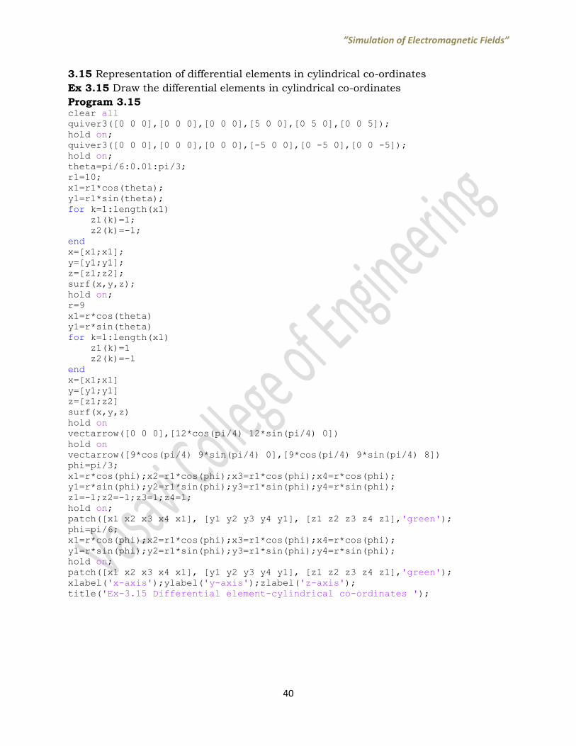
3.15 Representation of differential elements in cylindrical co-ordinates

Ex 3.15 Draw the differential elements in cylindrical co-ordinates

Program 3.15 clear all quiver3([0 0 0],[0 0 0],[0 0 0],[5 0 0],[0 5 0],[0 0 5]); hold on; quiver3([0 0 0],[0 0 0],[0 0 0],[-5 0 0],[0 -5 0],[0 0 -5]); hold on; theta=pi/6:0.01:pi/3; r1=10; x1=r1*cos(theta); y1=r1*sin(theta); for k=1:length(x1) z1(k)=1; z2(k)=-1; end x=[x1;x1]; y=[y1;y1]; z=[z1;z2]; surf(x,y,z); hold on; r=9 x1=r*cos(theta) y1=r*sin(theta) for k=1:length(x1) z1(k)=1 z2(k)=-1 end x=[x1;x1] y=[y1;y1] z=[z1;z2] surf(x,y,z) hold on vectarrow([0 0 0],[12*cos(pi/4) 12*sin(pi/4) 0]) hold on vectarrow([9*cos(pi/4) 9*sin(pi/4) 0],[9*cos(pi/4) 9*sin(pi/4) 8]) phi=pi/3; x1=r*cos(phi);x2=r1*cos(phi);x3=r1*cos(phi);x4=r*cos(phi); y1=r*sin(phi);y2=r1*sin(phi);y3=r1*sin(phi);y4=r*sin(phi); z1=-1;z2=-1;z3=1;z4=1; hold on; patch([x1 x2 x3 x4 x1], [y1 y2 y3 y4 y1], [z1 z2 z3 z4 z1],'green'); phi=pi/6; x1=r*cos(phi);x2=r1*cos(phi);x3=r1*cos(phi);x4=r*cos(phi); y1=r*sin(phi);y2=r1*sin(phi);y3=r1*sin(phi);y4=r*sin(phi); hold on; patch([x1 x2 x3 x4 x1], [y1 y2 y3 y4 y1], [z1 z2 z3 z4 z1],'green'); xlabel('x-axis');ylabel('y-axis');zlabel('z-axis'); title('Ex-3.15 Differential element-cylindrical co-ordinates ');


41

Fig 3.15 Differential element-Cylindrical co-ordinates


42

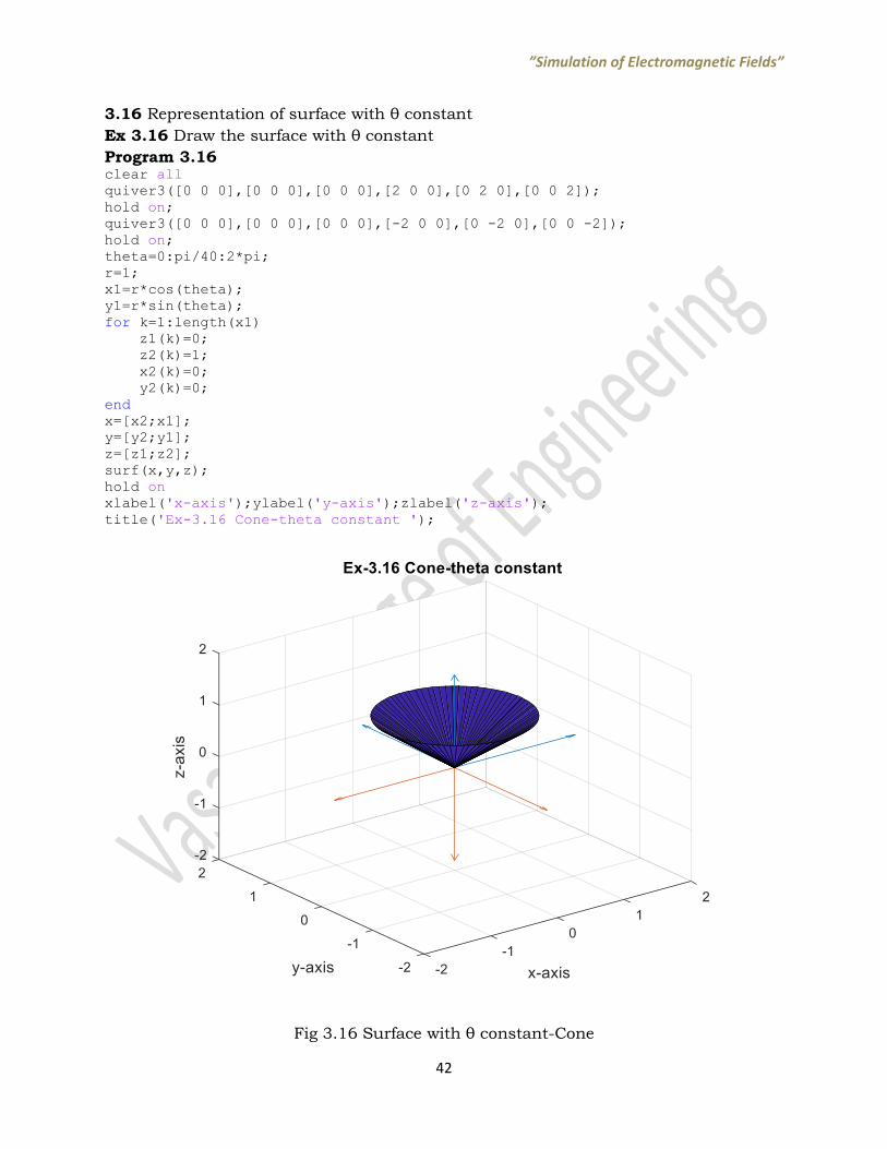
3.16 Representation of surface with θ constant

Ex 3.16 Draw the surface with θ constant

Program 3.16 clear all quiver3([0 0 0],[0 0 0],[0 0 0],[2 0 0],[0 2 0],[0 0 2]); hold on; quiver3([0 0 0],[0 0 0],[0 0 0],[-2 0 0],[0 -2 0],[0 0 -2]); hold on; theta=0:pi/40:2*pi; r=1; x1=r*cos(theta); y1=r*sin(theta); for k=1:length(x1) z1(k)=0; z2(k)=1; x2(k)=0; y2(k)=0; end x=[x2;x1]; y=[y2;y1]; z=[z1;z2]; surf(x,y,z); hold on xlabel('x-axis');ylabel('y-axis');zlabel('z-axis'); title('Ex-3.16 Cone-theta constant ');

Fig 3.16 Surface with θ constant-Cone


43

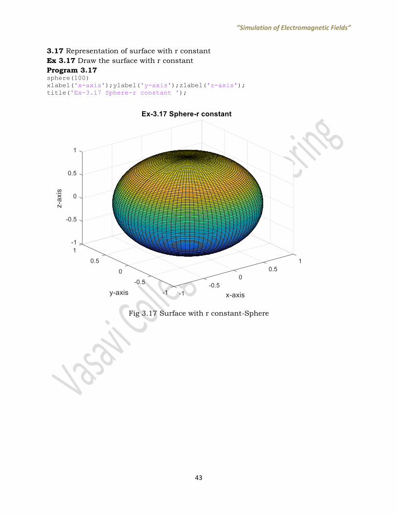
3.17 Representation of surface with r constant

Ex 3.17 Draw the surface with r constant

Program 3.17 sphere(100) xlabel('x-axis');ylabel('y-axis');zlabel('z-axis'); title('Ex-3.17 Sphere-r constant ');

Fig 3.17 Surface with r constant-Sphere


44

3.18 Representation of surfaces with r, θ and φ constant

Ex 3.18 Draw the surface with r, θ and φ constant

Program 3.18 clear all quiver3([0 0 0],[0 0 0],[0 0 0],[2 0 0],[0 2 0],[0 0 2]); hold on; quiver3([0 0 0],[0 0 0],[0 0 0],[-2 0 0],[0 -2 0],[0 0 -2]); hold on; theta=0:pi/40:2*pi; r=1; x1=r*cos(theta); y1=r*sin(theta); for k=1:length(x1) z1(k)=0;z2(k)=1;x2(k)=0;y2(k)=0; end x=[x2;x1];y=[y2;y1];z=[z1;z2]; surf(x,y,z); hold on; phi=pi/3; x1=0;x2=1.5*cos(phi);x3=1.5*cos(phi);x4=0; y1=0;y2=1.5*sin(phi);y3=1.5*sin(phi);y4=0; z1=-1.5;z2=-1.5;z3=1.5;z4=1.5; hold on; patch([x1 x2 x3 x4 x1], [y1 y2 y3 y4 y1], [z1 z2 z3 z4 z1],'green'); sphere(100); xlabel('x-axis');ylabel('y-axis');zlabel('z-axis'); title('Ex-3.18 r, theta and phi constant ');

Fig 3.18 Surface with r, θ and φ constant


45

3.19 Evaluation of surface and volume integrals of a cylinder

Ex 3.19 Evaluation of surface and volume integrals of a cylinder with given ,φ and z

Program 3.19 clc; %clear the command line clear; %removole all prevolious volariables VOLol=0; %initialize vololume of the closed surface to 0 % initialize the area of A1-A6 to 0

A1=0;

A2=0; A3=0; A4=0; A5=0;

A6=0; ro=4; %initialize ro to the its lower boundary z=8; %initialize z to the its lower boundary ang=pi/6;%initialize ang to the its lower boundary No_ro_values=100; %initialize the ro discretization No_ang_values=100;%initialize the ang discretization No_z_values=100;%initialize the z discretization dro=(4-2)/No_ro_values;%The ro increment dang=(pi/3-pi/9)/No_ang_values;%The ang increment dz=(5-3)/No_z_values;%The z increment %%the following routine calculates the vololume of the enclosed surface for k=1:No_z_values for j=1:No_ro_values for i=1:No_ang_values VOL=VOL+ro*dang*dro*dz;%add contribution to the vololume end ro=ro+dro;%p increases each time when z has been travoleled from its lower

boundary to its upper boundary end ro=2;%reset ro to its lower boundary end %%the following routine calculates the area of A1 and A2 ro1=2;%radius of A1 ro2=4;%radius of a2 for k=1:No_z_values for i=1:No_ang_values A1=A1+ro1*dang*dz;%get contribution to the the area of A1 A2=A2+ro2*dang*dz;%get contribution to the the area of A2 end end %%the following routing calculate the area of A3 and A4 ro=2;%reset ro to it's lower boundaty for j=1:No_ro_values for i=1:No_ang_values A3=A3+ro*dang*dro;%get contribution to the the area of A3 end ro=ro+dro;%p increases each time when ang has been travoleled from it's lower

boundary to it's upper boundary end A4=A3;%the area of A4 is equal to the area of A3 %%the following routing calculate the area of A5 and A6 for k=1:No_z_values


46

for j=1:No_ro_values A5=A5+dz*dro;%get contribution to the the area of A3 end end A6=A5;%the area of A6 is equal to the area of A6 Surface_area=A1+A2+A3+A4+A5+A6;%the area of the enclosed surface VOL Surface_area

Output

VOL = 8.3497

Surface_area = 24.7272


47


48

4. MATLAB Commands for Visualization of

Electromagnetic Fields

4.1 Use of meshgrid command

meshgrid Cartesian grid in 2-D/3-D space

[X,Y] = meshgrid(xgv,ygv) replicates the grid vectors xgv and ygv to produce the

coordinates of a rectangular grid (X, Y). The grid vector xgv is replicated

numel(ygv) times to form the columns of X. The grid vector ygv is replicated

numel(xgv) times to form the rows of Y.

[X,Y,Z] = meshgrid(xgv,ygv,zgv) replicates the grid vectors xgv, ygv, zgv to

produce the coordinates of a 3D rectangular grid (X, Y, Z). The grid vectors

xgv,ygv,zgv form the columns of X, rows of Y, and pages of Z respectively.

[x,y]=meshgrid(2,3)

x =

2

y =

3

>> [x,y]=meshgrid(2:4,3:5)


49

x =

2 3 4

2 3 4

2 3 4

y =

3 3 3

4 4 4

5 5 5

>> [x,y]=meshgrid(3:4,4:5)

x =

3 4

3 4

y =

4 4

5 5


50

>> [x,y]=meshgrid(3:4,3:5)

x =

3 4

3 4

3 4

y =

3 3

4 4

5 5

>> [x,y]=meshgrid(3:4,3:6)

x =

3 4

3 4

3 4

3 4

y =


51

3 3

4 4

5 5

6 6

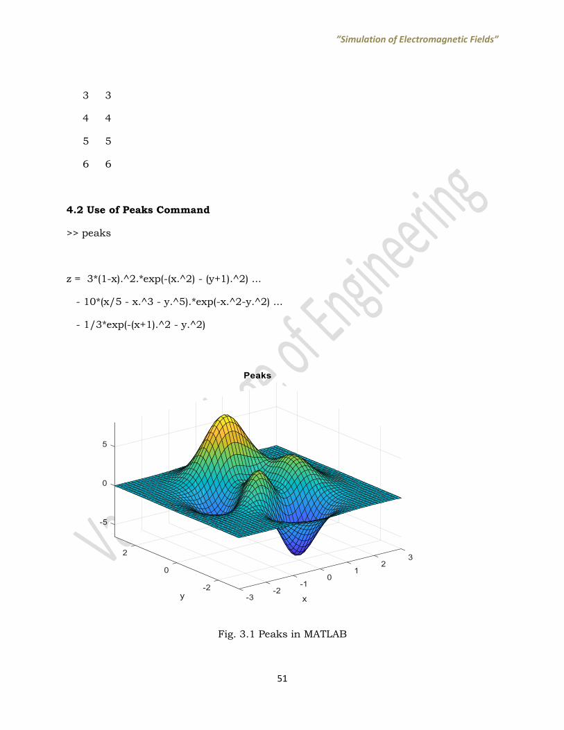
4.2 Use of Peaks Command

>> peaks

z = 3*(1-x).^2.*exp(-(x.^2) - (y+1).^2) ...

- 10*(x/5 - x.^3 - y.^5).*exp(-x.^2-y.^2) ...

- 1/3*exp(-(x+1).^2 - y.^2)

Fig. 3.1 Peaks in MATLAB


52

4.3 Divergnce:

Divergence: Divergence of a vector field.

DIV = divergence(X,Y,Z,U,V,W) computes the divergence of a 3-D vector field

U,V,W. The arrays X,Y,Z define the coordinates for U,V,W and must be

monotonic and 3-D plaid.

4.4 Contour:

Contour: Contour plot.

contour(Z) draws a contour plot of matrix Z in the x-y plane, with the x-

coordinates of the vertices corresponding to column indices of Z and the y-

coordinates corresponding to row indices of Z. The contour levels are chosen

automatically.

4.5 Evaluation of divergence of a vector K=10xax+6yay+10zaz

[X,Y,Z]= meshgrid(-2:.2:2, -2:.25:2, -2:.16:2);

U = 10*X;

V = 6*Y ;

W = 10*Z ;

div=divergence(X,Y,Z,U,V,W);

disp(div(1))

Output

26.0000

4.6 Calculate and plot the divergence of a vector field ( ⁄ )

where r=xax+yay

v=[-2:0.1:2];

[x,y]=meshgrid(v);

z=x;

r=sqrt(x.^2 + y.^2);


53

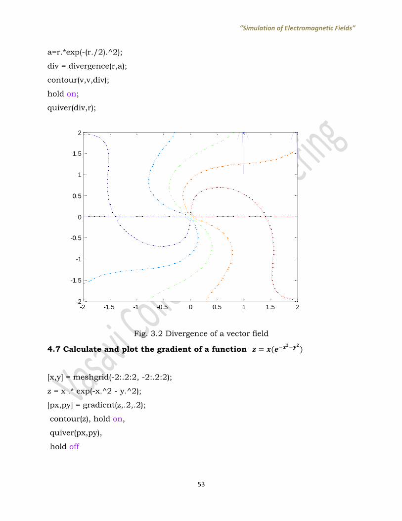
a=r.*exp(-(r./2).^2);

div = divergence(r,a);

contour(v,v,div);

hold on;

quiver(div,r);

Fig. 3.2 Divergence of a vector field

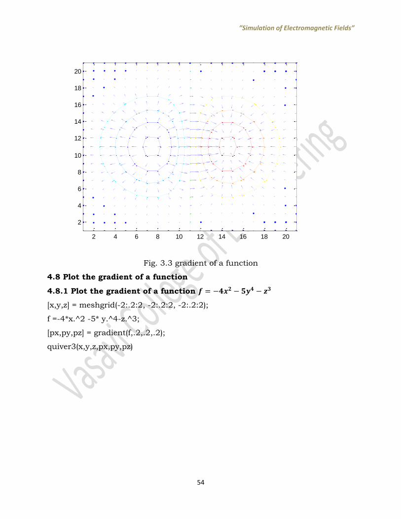
4.7 Calculate and plot the gradient of a function

[x,y] = meshgrid(-2:.2:2, -2:.2:2);

z = x .* exp(-x.^2 - y.^2);

[px,py] = gradient(z,.2,.2);

contour(z), hold on,

quiver(px,py),

hold off

-2 -1.5 -1 -0.5 0 0.5 1 1.5 2-2

-1.5

-1

-0.5

0

0.5

1

1.5

2


54

Fig. 3.3 gradient of a function

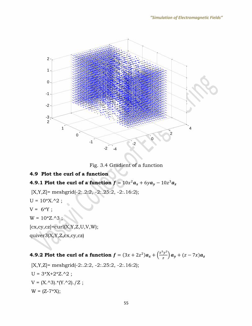
4.8 Plot the gradient of a function

4.8.1 Plot the gradient of a function

[x,y,z] = meshgrid(-2:.2:2, -2:.2:2, -2:.2:2);

f =-4*x.^2 -5* y.^4-z.^3;

[px,py,pz] = gradient(f,.2,.2,.2);

quiver3(x,y,z,px,py,pz)

2 4 6 8 10 12 14 16 18 20

2

4

6

8

10

12

14

16

18

20


55

Fig. 3.4 Gradient of a function

4.9 Plot the curl of a function

4.9.1 Plot the curl of a function

[X,Y,Z]= meshgrid(-2:.2:2, -2:.25:2, -2:.16:2);

U = 10*X.^2 ;

V = 6*Y ;

W = 10*Z.^3 ;

[cx,cy,cz]=curl(X,Y,Z,U,V,W);

quiver3(X,Y,Z,cx,cy,cz)

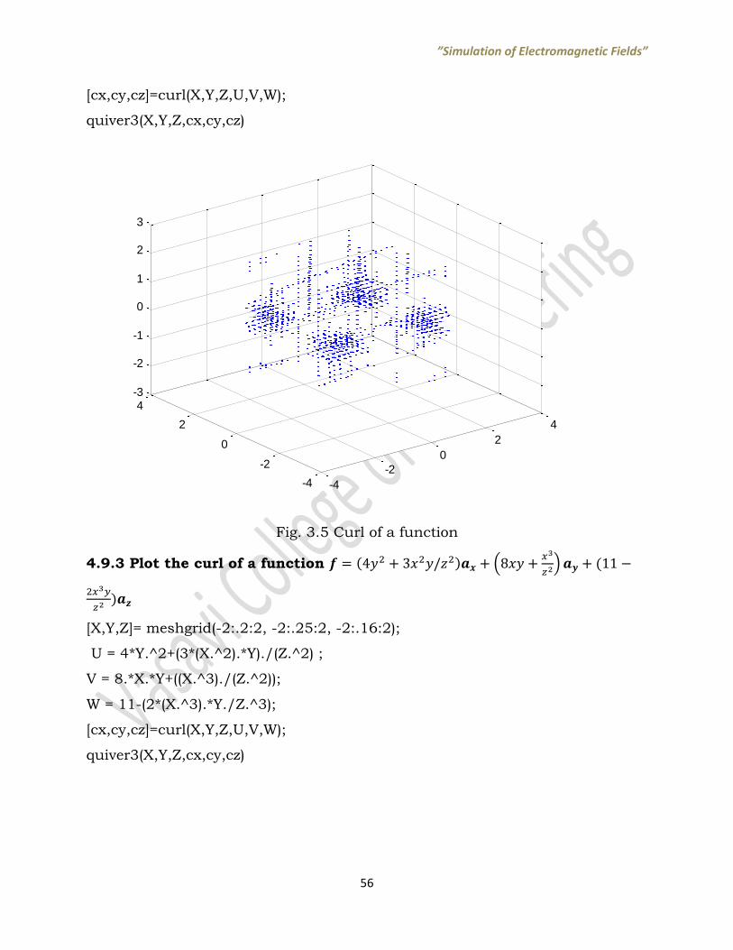
4.9.2 Plot the curl of a function (

)

[X,Y,Z]= meshgrid(-2:.2:2, -2:.25:2, -2:.16:2);

U = 3*X+2*Z.^2 ;

V = (X.^3).*(Y.^2)./Z ;

W = (Z-7*X);

-4

-2

0

2

4

-2

-1

0

1

2-3

-2

-1

0

1

2


56



Fig. 3.5 Curl of a function

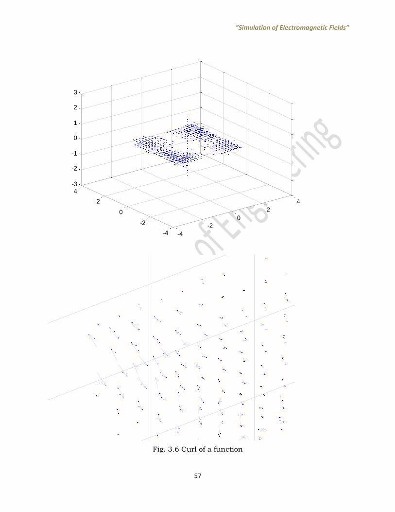
4.9.3 Plot the curl of a function (

)

[X,Y,Z]= meshgrid(-2:.2:2, -2:.25:2, -2:.16:2);

U = 4*Y.^2+(3*(X.^2).*Y)./(Z.^2) ;

V = 8.*X.*Y+((X.^3)./(Z.^2));

W = 11-(2*(X.^3).*Y./Z.^3);



-4

-2

0

2

4

-4

-2

0

2

4-3

-2

-1

0

1

2

3


57

Fig. 3.6 Curl of a function

-4

-2

0

2

4

-4

-2

0

2

4-3

-2

-1

0

1

2

3

-3

-2

-1

0

1

2

3

-2.5

-2

-1.5

-1

-0.5

0

0.5

1

1.5

2

2.5

-2

-1.5

-1

-0.5

0

0.5

1

1.5

2


58

5. Exercise Problems 1. Find the angle between the vectors A=10 ax+5ay ,B=12ax-2ay+3az using dot

product and cross product.

2. Given A=-4 ax+2ay+3az and B=3ax+4ay-az. Find the vector component of A

parallel to B.

3. Find the sum of P=3 ax+4ay+5az and T=-5ax+4ay-3az using parallelogram law of

addition.

4. Find the sum of Q=10 ax-6ay+8az and R=-ax+12ay-7az using triangular law of

addition.

5. Draw the position vector of points D(3,0,-5) and F(-9,2,-1).

6. Let A=-2ax+3ay+4az;B=7ax+ay+2az and C=-ax+2ay+4az.Find

i) AXB ii) (AXB).C iii) A.(BXC)

7. Given vectors A=ax+2ay+5az and B=5ax-ay+3az. Find the vector component of A

along B.

8. Show that vectors a = (4, 0,- 1) , b = (1,3, 4), and c = (-5,- 3,- 3) form the sides of a triangle.

9. If the position vectors of points T and S are 3ax-2ay+az and 4ax+6ay+2az find: (a) the coordinates of T and S, (b) the distance vector from T to S, (c) the distance between T and S.

10. Calculate the angles that vector H = 3ax + 5ay - 8az makes with the x-,y-, and z-axes.

For any queries please Contact:

Dr.G.Pranava Assistant Professor

EEE Department,VCE(A) [email protected]

9966744474

Dr.Ch.Ch.V.S.S.Sailaja Associate Professor

EEE Department,VCE(A) [email protected]

8121981253

Dr.M.Chakravarthy Professor,HoD EEE

[email protected] 9849979136

simulation of electromagnetic fields

Documents