simulation of blunt leading edge aerothermodynamics in ... · simulation of blunt leading edge ......

Simulation of Blunt Leading Edge Aerothermodynamics in Rarefied Hypersonic Flow

J. of the Braz. Soc. of Mech. Sci. & Eng. Copyright 2007 by ABCM April-June 2007, Vol. XXIX, No. 2 /123

Wilson F. N. Santos Member, ABCM

[email protected] Combustion and Propulsion Laboratory

National Institute for Space Research - INPE 12630-000 Cachoeira Paulista, SP. Brazil

Simulation of Blunt Leading Edge Aerothermodynamics in Rarefied Hypersonic Flow The steady-state aerodynamic characteristics of a new family of blunted leading edges immersed in a high-speed rarefied air flow are examined by using a Direct Simulation Monte Carlo (DSMC) Method. A very detailed description of the flow properties has been presented separately at the vicinity of the nose and adjacent to the afterbody surface of the leading edges by a numerical method that properly accounts for non-equilibrium effects that arise near the leading edges and that are especially important at high Mach number. Comparisons based on geometry are made between these new blunt configurations and round leading edge. Some significant differences between these leading edges are noted on the flowfield structure and on the aerodynamic surface quantities. It is found that the upstream effects have different influence on velocity, density, pressure and temperature along the stagnation streamline ahead of the leading edges. The analysis also shows that, despite the seeming advantages of the new blunt leading edge shapes, round leading edge still provides smaller stagnation point heating. Nevertheless, round leading edge provides larger total drag than the new blunt shapes under the range of condition investigated. Keywords: hypersonic flow, rarefied flow, DSMC, blunt leading edge, sharp leading edge

Introduction

At hypersonic flight speeds, the vehicle leading edge must be blunt to some extent in order to reduce the heat transfer rate to acceptable levels and to allow for internal heat conduction. The use of blunt-nose shapes tends to alleviate the aerodynamic heating problem since the heat flux for blunt bodies is far lower than that for sharply pointed bodies. In addition, the reduction in heating rate for a blunt body is accompanied by an increase in heat capacity, due to the increased volume. Due mainly to manufacturing problems and the extremely high temperatures attained in hypersonic flight, hypersonic vehicles will have blunt nose, although probably slendering out at a short distance from the nose. Therefore, designing a hypersonic vehicle leading edge involves a tradeoff between making the leading edge sharp enough to obtain acceptable aerodynamic and propulsion efficiency and blunt enough to reduce the aerodynamic heating at the stagnation point.

Usually, a round leading edge with constant radius of curvature (circular cylinder) near the stagnation point has been chosen for blunting geometry. Nevertheless, shock detachment distance on a cylinder, with associated leakage, scales with the radius of curvature. Certain classes of non-circular shapes may provide the required bluntness with smaller shock separation than round leading edges, thus allowing manufacturing, and ultimately heating control, with reduced aerodynamic losses. In this connection, a typical blunt body, composed of a flat nose followed by a highly curved, but for the most part slightly inclined afterbody surface, may provide the required bluntness for heat transfer, manufacturing and handling concerns with reduced departures from ideal aerodynamic performance. This concept is based on work of Reller (1957), who has pointed out that this shape results from a method of designing low heat transfer bodies. According to Reller (1957), low heat transfer bodies are devised on the premise that the rate of heat transfer to the nose will be low if the local velocity is low, while the rate of heat transfer to the afterbody will be low if the local density is low.1

In this scenario, the purpose of this work is to examine computationally the flowfield structure and the aerodynamic surface quantities for a family of these contours, flat-nose leading edges.

Paper accepted January, 2007. Technical Editor: Olympio A. de Faria Mello.

Both the flowfield properties upstream of the leading edge of a body and the state of the gas adjacent to the body surface are affected by molecules reflected from the edge region. The degree of the effect is in part conditioned by the edge geometry. Therefore, the effect of the flat-face thickness on the flowfield structure and on the aerodynamic surface quantities will be investigated for a range of Knudsen number, based on the thickness of the leading edge, covering from the transitional flow regime to the free molecular flow regime.

In a first stage, in the present account, the aerodynamic performance of these flat-nose leading edges will be compared to round leading edge in order to provide information on how well these shapes stand up as possible candidates for blunting geometries of hypersonic leading edges, such as hypersonic waveriders (Nonweiler, 1959), which have been considered for high-altitude/low-density applications (Anderson, 1990, Potter and Rockaway, 1994, Rault, 1994, Graves and Argrow, 2001, Shvets et al., 2005). In a second stage, in a future account, the aerodynamic performance of these flat-nose leading edges will be compared to other non-circular shapes, such as power-law shaped leading edges (Santos, 2005a, and Santos and Lewis, 2002, 2005a and 2005b).

The focus of the present study is the low-density region in the upper atmosphere, where numerical gaskinetic procedures are available to simulate hypersonic flows. High-speed flows under low-density conditions deviate from a perfect gas behavior because of the excitation of rotation, vibration and possibly dissociation. At high altitude, and therefore low density, the molecular collision rate is low and the energy exchange occurs under non-equilibrium conditions. In such a circumstance, the degree of molecular non-equilibrium is such that the Navier-Stokes equations are inappropriate. Therefore, a Direct Simulation Monte Carlo (DSMC) method will be employed to calculate the rarefied hypersonic two-dimensional flow on the flat-nose leading edges.

Nomenclature

a = speed of sound, m/s Cd = drag coefficient, Eq. (10) Cf = skin friction coefficient, Eq. (7) Ch = heat transfer coefficient, Eq. (3) Cp = pressurer coefficient, Eq. (5) c = molecular velocity, m/s e =specific energy, J/kg

Wilson F. N. Santos

/ Vol. XXIX, No. 2, April-June 2007 ABCM124

F = drag force, N H = body height at the base, m k = exponent, Eq. (1) Kn = Knudsen number, λ/l L = body length, m l = characteristic length, m M = Mach number, V/a m = mass, kg N = number of molecules, dimensionless n = number densty, m-3

p = pressure, N/m2

q = heat flux, W/m2

R = circular cylinder radius, m Re = Reynolds number, ρVl/µs = arc length, m S = dimensionless arc length, s/λ∞t = leading-edge thickness, m T = temperature, K V = velocity, m/s x = cartesian axis in physical space, m y = cartesian axis in physical space, m ynose = half leading-edge thickness, m

Greek Symbols

η = coordinate normal to body surface, mξ = coordinate tangent to body surface, m λ = mean free path, m ζ = degree of freedom, dimensionless θ = wedge angle, body slope angle, degree τ =shear stress, N/m2

µ = dynamic viscosity, kg/(m s)ρ = density, kg/m3

Subscripts

i relative to incident molecule o relative to overall r relative to reflected molecule R relative to rotational T relative to translational V relative to vibrationalw wall conditions∞ freestream conditions

Body-Shape Definition

In dimensionless form, the contour that defines the shape of the afterbody surface is given by the following equation,

ydyx noseyy

yk

∫== −=

01 (1)

where noseyxx = and noseyyy = .

The flat-nose leading edges are modeled by assuming a sharp leading edge of half angle θ with a circular cylinder of radius Rinscribed tangent to the wedge. The blunt leading edges, inscribed between the wedge and the cylinder, are also tangent to them at the same common point where they have the same slope angle. The circular cylinder diameter provides a reference for the amount of blunting desired on the leading edges. It was assumed a leading edge half angle of 10 degrees, a circular cylinder diameter of 10-2m and flat-face thickness t/λ∞ of 0.01, 0.1 and 1, where t = 2ynose and λ∞ is the freestream mean free path. Figure 1 illustrates this construction for the set of leading edges investigated. From geometric considerations, the exponent k in Eq. (1) is obtained by matching slope on the wedge, circular cylinder and on the body

shapes at the tangency point. For dimensionless thickness t/λ∞ of 0.01, 0.1 and 1, the exponent k corresponds to 0.501, 0.746 and 1.465, respectively. The common body height H and the body length L are obtained in a straightforward manner. It was assumed that the leading edges are infinitely long but only the length L is considered, since the wake region behind the leading edges is not of interest in this investigation.

Computational Method and Procedure

The most successful numerical technique for modeling complex transitional flows has been the DSMC method (Bird, 1994) introduced by Bird in 1960’s. The DSMC method simulates real gas flows with various physical processes by means of a huge number of modeling particles, where each particle represents a fixed number of real gas particles. In the DSMC model, the particle evolution is divided into two independent phases during the simulation; the movement phase and the collision phase. In the movement phase, all particles are moved over distances appropriate to a short time interval, time step, and some of them interact with the domain boundaries in this time interval. Particles that strike the solid wall would reflect according to the appropriate gas-surface interaction model, specular, diffusive or a combination of these. In the collision phase, intermolecular collisions are performed according to the theory of probability without time being consumed. In this way, the intermolecular collisions are uncoupled to the translational molecular motion over the time step used to advance the simulation. Time is advanced in discrete steps such that each step is small in comparison with the mean collision time (Hadjiconstantinou, 2000, and Garcia and Wagner, 2000). The simulation is always calculated as unsteady flow. However, a steady flow solution is obtained as the large time state of the simulation.

θt = 1.0λ∞0.1λ∞

0.01λ∞

Wedge

Tangency point

Cylinder

L

HR

x

Figure 1. Drawing illustrating the leading edge geometry.

The molecular collisions are modeled by using the variable hard sphere (VHS) molecular model (Bird, 1981) and the no time counter (NTC) collision sampling technique (Bird, 1989). The energy exchange between kinetic and internal modes is controlled by the Borgnakke-Larsen statistical model (Borgnakke and Larsen, 1975). Simulations are performed using a non-reacting gas model consisting of two chemical species, N2 and O2. Energy exchanges between the translational and internal modes, rotational and vibrational, are considered. Relaxation collision numbers of 5 and 50 were used for the calculations of rotation and vibration, respectively.

In order to easily account for particle-particle collisions, the flowfield is divided into an arbitrary number of regions, which are subdivided into computational cells. The cells are further subdivided into subcells. The cell provides a convenient reference sampling of the macroscopic gas properties, while the collision partners are selected from the same subcell for the establishment of the collision rate. In the DSMC algorithm, the linear dimensions of the cells should be small in comparison with the scale length of the



macroscopic flow gradients normal to streamwise directions, which means that the cell dimensions should be of the order of or smaller than the local mean free path (Alexander et al., 1998 and 2000).

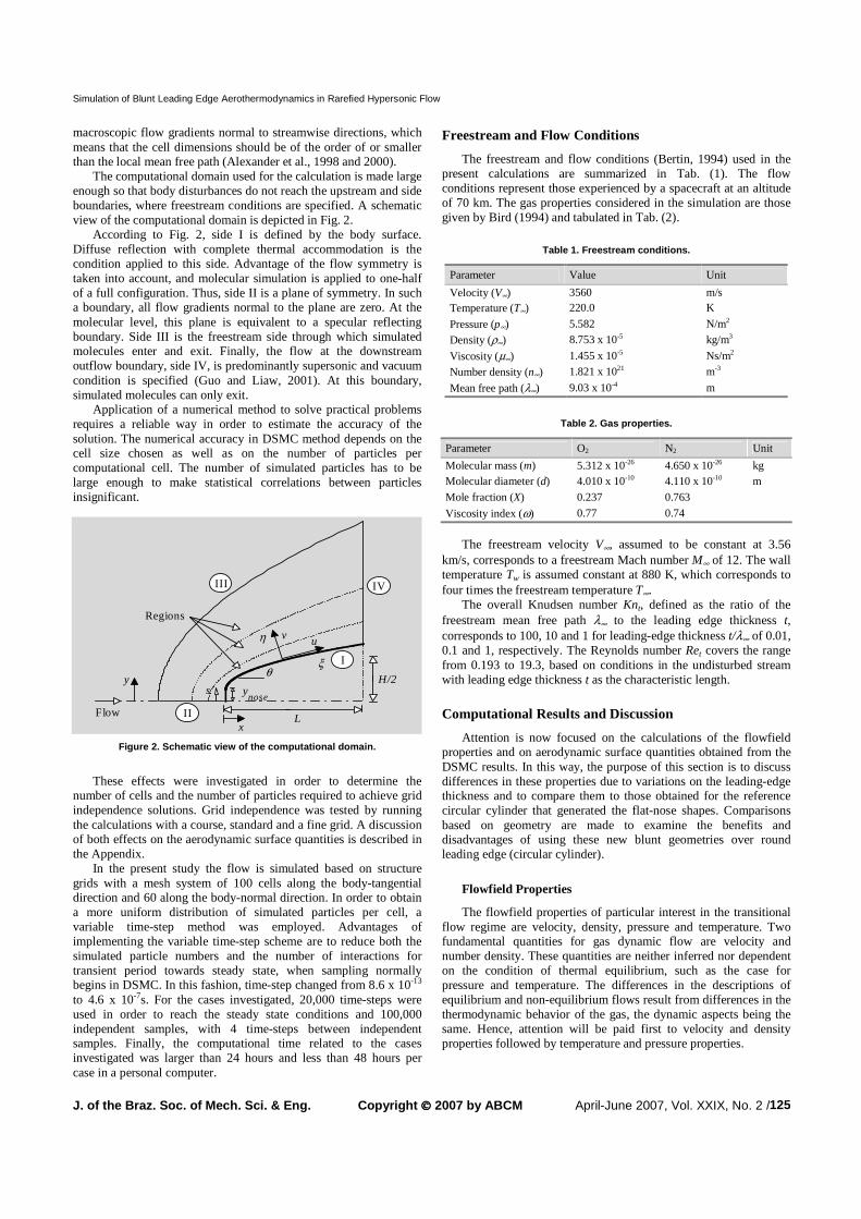
The computational domain used for the calculation is made large enough so that body disturbances do not reach the upstream and side boundaries, where freestream conditions are specified. A schematic view of the computational domain is depicted in Fig. 2.

According to Fig. 2, side I is defined by the body surface. Diffuse reflection with complete thermal accommodation is the condition applied to this side. Advantage of the flow symmetry is taken into account, and molecular simulation is applied to one-half of a full configuration. Thus, side II is a plane of symmetry. In such a boundary, all flow gradients normal to the plane are zero. At the molecular level, this plane is equivalent to a specular reflecting boundary. Side III is the freestream side through which simulated molecules enter and exit. Finally, the flow at the downstream outflow boundary, side IV, is predominantly supersonic and vacuum condition is specified (Guo and Liaw, 2001). At this boundary, simulated molecules can only exit.

Application of a numerical method to solve practical problems requires a reliable way in order to estimate the accuracy of the solution. The numerical accuracy in DSMC method depends on the cell size chosen as well as on the number of particles per computational cell. The number of simulated particles has to be large enough to make statistical correlations between particles insignificant.

I

II

III IV

xL

y

η

ξ

v u

θH/2

Regions

Flow

s ynose

Figure 2. Schematic view of the computational domain.

These effects were investigated in order to determine the number of cells and the number of particles required to achieve grid independence solutions. Grid independence was tested by running the calculations with a course, standard and a fine grid. A discussion of both effects on the aerodynamic surface quantities is described in the Appendix.

In the present study the flow is simulated based on structure grids with a mesh system of 100 cells along the body-tangential direction and 60 along the body-normal direction. In order to obtain a more uniform distribution of simulated particles per cell, a variable time-step method was employed. Advantages of implementing the variable time-step scheme are to reduce both the simulated particle numbers and the number of interactions for transient period towards steady state, when sampling normally begins in DSMC. In this fashion, time-step changed from 8.6 x 10-13

to 4.6 x 10-7s. For the cases investigated, 20,000 time-steps were used in order to reach the steady state conditions and 100,000 independent samples, with 4 time-steps between independent samples. Finally, the computational time related to the cases investigated was larger than 24 hours and less than 48 hours per case in a personal computer.

Freestream and Flow Conditions

The freestream and flow conditions (Bertin, 1994) used in the present calculations are summarized in Tab. (1). The flow conditions represent those experienced by a spacecraft at an altitude of 70 km. The gas properties considered in the simulation are those given by Bird (1994) and tabulated in Tab. (2).

Table 1. Freestream conditions.

Parameter Value Unit

Velocity (V∞) 3560 m/s Temperature (T∞) 220.0 K

Pressure (p∞) 5.582 N/m2

Density (ρ∞) 8.753 x 10-5 kg/m3

Viscosity (µ∞) 1.455 x 10-5 Ns/m2

Number density (n∞) 1.821 x 1021 m-3

Mean free path (λ∞) 9.03 x 10-4 m

Table 2. Gas properties.

Parameter O2 N2 Unit

Molecular mass (m) 5.312 x 10-26 4.650 x 10-26 kg Molecular diameter (d) 4.010 x 10-10 4.110 x 10-10 m

Mole fraction (X) 0.237 0.763

Viscosity index (ω) 0.77 0.74

The freestream velocity V∞, assumed to be constant at 3.56 km/s, corresponds to a freestream Mach number M∞ of 12. The wall temperature Tw is assumed constant at 880 K, which corresponds to four times the freestream temperature T∞.

The overall Knudsen number Knt, defined as the ratio of the freestream mean free path λ∞ to the leading edge thickness t, corresponds to 100, 10 and 1 for leading-edge thickness t/λ∞ of 0.01, 0.1 and 1, respectively. The Reynolds number Ret covers the range from 0.193 to 19.3, based on conditions in the undisturbed stream with leading edge thickness t as the characteristic length.

Computational Results and Discussion

Attention is now focused on the calculations of the flowfield properties and on aerodynamic surface quantities obtained from the DSMC results. In this way, the purpose of this section is to discuss differences in these properties due to variations on the leading-edge thickness and to compare them to those obtained for the reference circular cylinder that generated the flat-nose shapes. Comparisons based on geometry are made to examine the benefits and disadvantages of using these new blunt geometries over round leading edge (circular cylinder).

Flowfield Properties

The flowfield properties of particular interest in the transitional flow regime are velocity, density, pressure and temperature. Two fundamental quantities for gas dynamic flow are velocity and number density. These quantities are neither inferred nor dependent on the condition of thermal equilibrium, such as the case for pressure and temperature. The differences in the descriptions of equilibrium and non-equilibrium flows result from differences in the thermodynamic behavior of the gas, the dynamic aspects being the same. Hence, attention will be paid first to velocity and density properties followed by temperature and pressure properties.

Wilson F. N. Santos


Velocity Profile

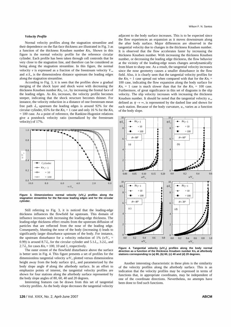
Normal velocity profiles along the stagnation streamline and their dependence on the flat-face thickness are illustrated in Fig. 3 as a function of the thickness Knudsen number Knt. Shown in this figure is the normal velocity profile for the reference circular cylinder. Each profile has been taken through cell centroids that lie very close to the stagnation line, and therefore can be considered as being along the stagnation streamline. In this figure, the normal velocity v is expressed as a fraction of the freestream velocity V∞, and x/λ∞ is the dimensionless distance upstream the leading edges along the stagnation streamline.

According to Fig. 3, it is seen that the profiles show a gradual merging of the shock layer and shock wave with decreasing the thickness Knudsen number Knt, i.e., by increasing the frontal face of the leading edges. As Knt increases, the velocity profile becomes steeper, indicating that the shock structure becomes thinner. For instance, the velocity reduction in a distance of one freestream mean free path λ∞ upstream the leading edges is around 92% for the circular cylinder, 65% for the Knt = 1 case and only 16 % for the Knt

= 100 case. As a point of reference, the Rankine-Hugoniot relations give a postshock velocity ratio (normalized by the freestream velocity) of 17%.

0.0

0.2

0.4

0.6

0.8

1.0

10.0 8.0 6.0 4.0 2.0 0.0

Cylinder

= 1

= 10

= 100

Knt

-x/λ∞

Figure 3. Dimensionless normal velocity (v/V∞∞∞∞) profiles along the stagnation streamline for the flat-nose leading edges and for the circular cylinder.

Still referring to Fig. 3, it is noticed that the leading-edge thickness influences the flowfield far upstream. This domain of influence increases with increasing the leading-edge thickness. The leading-edge thickness effect results from the upstream diffusion of particles that are reflected from the nose of the leading edge. Consequently, blunting the nose of the body (increasing t) leads to significantly larger disturbance upstream of the body. For instance, the upstream disturbance for a velocity reduction of 1% (v/V∞ = 0.99) is around 8.7λ∞ for the circular cylinder and 5.1λ∞, 3.2λ∞ and 2.7λ∞ for cases Knt = 100, 10 and 1, respectively.

The outer extent of the flowfield disturbance above the surface is better seen in Fig. 4. This figure presents a set of profiles for the dimensionless tangential velocity u/V∞ plotted versus dimensionless height away from the body surface η/λ∞ and parameterized by the body slope angle θ along the afterbody surface. In an effort to emphasize points of interest, the tangential velocity profiles are shown for four stations along the afterbody surface represented by the body slope angles of 80, 60, 40 and 20 degrees.

Interesting features can be drawn from this set of tangential velocity profiles. As the body slope decreases the tangential velocity

adjacent to the body surface increases. This is to be expected since the flow experiences an expansion as it moves downstream along the after body surface. Major differences are observed in the tangential velocity due to changes in the thickness Knudsen number. It is observed that the flow accelerates faster by increasing the thickness Knudsen number. With increasing the thickness Knudsen number, or decreasing the leading edge thickness, the flow behavior at the vicinity of the leading-edge noses changes aerodynamically from blunt to sharp one. As a result, the tangential velocity increases since the nose geometry causes a smaller disturbance in the flow field. Also, it is clearly seen that the tangential velocity profiles for the Knt = 1 case spread out when compared with that for the Knt = 100 case, indicating the flow expansion along the body surface for Knt = 1 case is much slower than that for the Knt = 100 case. Furthermore, of great significance in this set of diagrams is the slip velocity. The slip velocity increases with increasing the thickness Knudsen number. It should be noted that the tangential velocity u∞, defined as η → ∞, is represented by the dashed line and shown for each station. Because of the body curvature, u∞ varies as a function of the body slope.

0

2

4

6

8

10

0.00 0.05 0.10 0.15 0.20

= 1

= 10

= 100

θ = 80o

Knt

(a)

η/λ∞

u/V∞

0

2

4

6

8

10

0.0 0.2 0.4 0.6

= 1

= 10

= 100

θ = 60o

Knt

(b)

η/λ∞

u/V∞

0

2

4

6

8

10

0.0 0.2 0.4 0.6 0.8

= 1

= 10

= 100

θ = 40o

Knt

(c)

η/λ∞

u/V∞

0

2

4

6

8

10

0.0 0.2 0.4 0.6 0.8 1.0

= 1

= 10

= 100

θ = 20o

Knt

(d)

η/λ∞

u/V∞

Figure 4. Tangential velocity (u/V∞∞∞∞) profiles along the body normal direction as a function of the thickness Knudsen number Knt at afterbody stations corresponding to (a) 80, (b) 60, (c) 40 and (d) 20 degrees.

Another interesting characteristic in these plots is the similarity of the velocity profiles along the afterbody surface. This is an indication that the velocity profiles may be expressed in terms of functions that, in appropriate coordinates, may be independent of one of the coordinate directions. Nevertheless, no attempts have been done to find such functions.



Density Profile

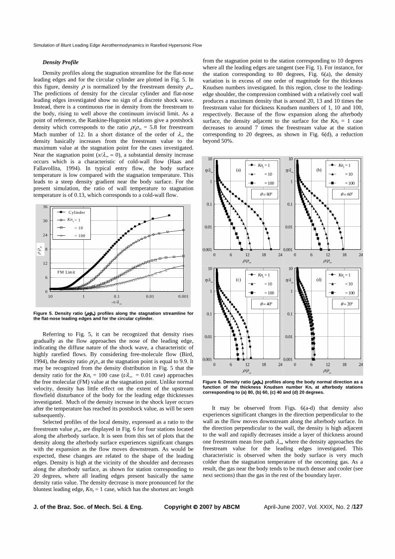
Density profiles along the stagnation streamline for the flat-nose leading edges and for the circular cylinder are plotted in Fig. 5. In this figure, density ρ is normalized by the freestream density ρ∞. The predictions of density for the circular cylinder and flat-nose leading edges investigated show no sign of a discrete shock wave. Instead, there is a continuous rise in density from the freestream to the body, rising to well above the continuum inviscid limit. As a point of reference, the Rankine-Hugoniot relations give a postshock density which corresponds to the ratio ρ/ρ∞ = 5.8 for freestream Mach number of 12. In a short distance of the order of λ∞ the density basically increases from the freestream value to the maximum value at the stagnation point for the cases investigated. Near the stagnation point (x/λ∞ ≈ 0), a substantial density increase occurs which is a characteristic of cold-wall flow (Haas and Fallavollita, 1994). In typical entry flow, the body surface temperature is low compared with the stagnation temperature. This leads to a steep density gradient near the body surface. For the present simulation, the ratio of wall temperature to stagnation temperature is of 0.13, which corresponds to a cold-wall flow.

0

6

12

18

24

30

36

10 1 0.1 0.01 0.001

Cylinder

= 1

= 10

= 100

Knt

-x/λ∞

FM Limit

Figure 5. Density ratio (ρρρρ⁄⁄⁄⁄ρρρρ∞∞∞∞) profiles along the stagnation streamline for the flat-nose leading edges and for the circular cylinder.

Referring to Fig. 5, it can be recognized that density rises gradually as the flow approaches the nose of the leading edge, indicating the diffuse nature of the shock wave, a characteristic of highly rarefied flows. By considering free-molecule flow (Bird, 1994), the density ratio ρ/ρ∞ at the stagnation point is equal to 9.9. It may be recognized from the density distribution in Fig. 5 that the density ratio for the Knt = 100 case (t⁄λ∞ = 0.01 case) approaches the free molecular (FM) value at the stagnation point. Unlike normal velocity, density has little effect on the extent of the upstream flowfield disturbance of the body for the leading edge thicknesses investigated. Much of the density increase in the shock layer occurs after the temperature has reached its postshock value, as will be seen subsequently.

Selected profiles of the local density, expressed as a ratio to the freestream value ρ∞, are displayed in Fig. 6 for four stations located along the afterbody surface. It is seen from this set of plots that the density along the afterbody surface experiences significant changes with the expansion as the flow moves downstream. As would be expected, these changes are related to the shape of the leading edges. Density is high at the vicinity of the shoulder and decreases along the afterbody surface, as shown for station corresponding to 20 degrees, where all leading edges present basically the same density ratio value. The density decrease is more pronounced for the bluntest leading edge, Knt = 1 case, which has the shortest arc length

from the stagnation point to the station corresponding to 10 degrees where all the leading edges are tangent (see Fig. 1). For instance, for the station corresponding to 80 degrees, Fig. 6(a), the density variation is in excess of one order of magnitude for the thickness Knudsen numbers investigated. In this region, close to the leading-edge shoulder, the compression combined with a relatively cool wall produces a maximum density that is around 20, 13 and 10 times the freestream value for thickness Knudsen numbers of 1, 10 and 100, respectively. Because of the flow expansion along the afterbody surface, the density adjacent to the surface for the Knt = 1 case decreases to around 7 times the freestream value at the station corresponding to 20 degrees, as shown in Fig. 6(d), a reduction beyond 50%.

0.001

0.01

0.1

1

10

0 6 12 18 24

= 1

= 10

= 100

θ = 80o

Knt(a)η/λ∞

ρ/ρ∞

0.001

0.01

0.1

1

10

0 6 12 18 24

= 1

= 10

= 100

θ = 60o

Knt(b)η/λ∞

ρ/ρ∞

0.001

0.01

0.1

1

10

0 6 12 18 24

= 1

= 10

= 100

θ = 40o

Knt(c)η/λ∞

ρ/ρ∞

0.001

0.01

0.1

1

10

0 6 12 18 24

= 1

= 10

= 100

θ = 20o

Knt(d)η/λ

∞

ρ/ρ∞

Figure 6. Density ratio (ρρρρ⁄⁄⁄⁄ρρρρ∞∞∞∞) profiles along the body normal direction as a function of the thickness Knudsen number Knt at afterbody stations corresponding to (a) 80, (b) 60, (c) 40 and (d) 20 degrees.

It may be observed from Figs. 6(a-d) that density also experiences significant changes in the direction perpendicular to the wall as the flow moves downstream along the afterbody surface. In the direction perpendicular to the wall, the density is high adjacent to the wall and rapidly decreases inside a layer of thickness around one freestream mean free path λ∞, where the density approaches the freestream value for the leading edges investigated. This characteristic is observed when the body surface is very much colder than the stagnation temperature of the oncoming gas. As a result, the gas near the body tends to be much denser and cooler (see next sections) than the gas in the rest of the boundary layer.

Wilson F. N. Santos


Temperature Profile

The strong shock wave that forms ahead of a blunt leading edge at hypersonic flow converts part of the kinetic energy of the freestream air molecules into thermal energy. This thermal energy downstream of the shock wave is partitioned into increasing the translational kinetic energy of the air molecules, and into exciting of other molecular energy states such as rotation and vibration.

Kinetic temperature profiles along the stagnation streamline are demonstrated in Figs. 7 and 8 for thickness Knudsen number of 100 and 1, respectively. Kinetic temperature profiles for thickness Knudsen number of 10 are intermediate to those for Knt of 100 and 1 and, therefore, they are not shown. For comparison purpose, Fig. 9 illustrates the kinetic temperature profiles for the reference circular cylinder. In these figures, temperature ratio accounts for the kinetic temperatures normalized by the freestream temperature T∞. It is apparent from this set of figures that thermodynamic non-equilibrium occurs throughout the shock layer, as shown by the lack of equilibrium of the translational and internal kinetic temperatures. Thermal non-equilibrium occurs when the temperatures associated with the translational, rotational, and vibrational modes of a polyatomic gas are different.

The overall kinetic temperature shown is defined for a non-equilibrium gas as the weighted mean of the translational and internal temperature (Bird, 1994) as follows,

VRT

VVRRTTo

TTTT

ζζζζζζ

++++

= (2)

where ζ is the degree of freedom, and subscripts T, R and V stand for translational, rotational and vibrational modes.

The overall kinetic temperature is equivalent to the thermodynamic temperature only under thermal equilibrium conditions. In this way, it should be emphasized that the ideal gas equation of state does not apply to this temperature in a non-equilibrium situation.

Referring to Figs. 7, 8 and 9, in the undisturbed freestream far from the nose of the leading edges, the translational and internal kinetic temperatures have basically the same value and are equal to the thermodynamic temperature. Approaching the nose of the leading edges, the translational kinetic temperature rises to well above the rotational and vibrational temperatures and reaches a maximum value that is a function of the leading edge thickness. For comparison purpose, the maximum value (TT/T∞) is around 24.7, 28, 28.8, and 31.8 for leading edges given by Knt of 100, 10, and 1 and the circular cylinder, respectively. Since a large number of collisions is needed to excite molecules vibrationally from the ground state to the upper state, the vibrational temperature increases much more slowly than rotational temperature. Still further downstream toward the nose of the leading edges, the translational kinetic temperature decreases and reaches a value on the wall that is above the wall temperature, resulting in a temperature jump as defined in continuum formulation.

The substantial rise in translational kinetic temperature for blunt leading edges occurred before the density rise, as shown in Fig. 5. For instance, the kinetic translational temperature reaches the maximum value around a distance of one freestream mean free path from the nose of the leading edge for the Knt = 1 case, while the density ratio ρ⁄ρ∞ is around 2.4 at the same station. The translational kinetic temperature rise for blunt leading edges results from the essentially bimodal velocity distribution (Liepmann et al., 1964): the molecular sample consisting of mostly undisturbed freestream molecules with the molecules that have been affected by the shock and reflected from the body. In this connection, the translational

kinetic temperature rise is a consequence of the large velocity separation between these two classes of molecules.

0

8

16

24

32

10 1 0.1 0.01 0.001

Translational

Rotational

Vibrational

Overall

Knt = 100

-x/λ∞

Figure 7. Kinetic temperature ratio (T⁄⁄⁄⁄T∞∞∞∞) profiles along the stagnation streamline for thickness Knudsen number Knt of 100.

0

8

16

24

32

10 1 0.1 0.01 0.001

Translational

Rotational

Vibrational

Overall

Knt = 1

-x/λ∞

Figure 8. Kinetic temperature ratio (T⁄⁄⁄⁄T∞∞∞∞) profiles along the stagnation streamline for thickness Knudsen number Knt of 1.

0

8

16

24

32

20 10 1 0.1 0.01 0.001

Translational

Rotational

Vibrational

Overall

Cylinder

−x/λ∞

Figure 9. Kinetic temperature ratio (T⁄⁄⁄⁄T∞∞∞∞) profiles along the stagnation streamline for the circular cylinder.



The difference between translational temperature and the internal temperatures close to the stagnation point region also indicates that the thermodynamic equilibrium is not achieved in the boundary layer. The difference between the temperature components in the shock layer decreases as thickness Knudsen number decreases, i.e., as the leading edge becomes blunt, since the collision rate increases because of the higher density (see Fig. 5). The vibrational temperature increases much more slowly as the thickness Knudsen number increases. As this process is density dependent, the differences between the translational kinetic temperature and vibrational temperature increases as the leading edges become sharp.

Particular attention is paid to the overall kintetic temperature in the shock layer. In this respect, the overall kinetic temperature variation is taken normal to the body surface at afterbody stations corresponding to 80, 60, 40 and 20 degrees.

Figure 10 depicts profiles of overall kinetic temperatures as a function of the thickness Knudsen number Knt at the considered positions normal to the afterbody surface along the η-axis. According to this set of plots, it is observed that the downstream evolution of the flow displays a smearing tendency of the shock wave due to the displacement of the maximum value for the overall kinetic temperature. Also, it may be recognized from the temperature distribution in Fig. 10 that significant changes in the overall kinetic temperature profiles occur within a larger layer adjacent to the body surface compared to that for density.

To /T∞

0.001

0.01

0.1

1

10

0 4 8 12 16 20

= 1

= 10

= 100

θ = 80o

Knt

(a)η/λ∞

To /T∞

0.001

0.01

0.1

1

10

0 4 8 12 16 20

= 1

= 10

= 100

θ = 60o

Knt

(b)η/λ∞

To /T∞

0.001

0.01

0.1

1

10

0 4 8 12 16 20

= 1

= 10

= 100

θ = 40o

Knt

(c)η/λ∞

To /T∞

0.001

0.01

0.1

1

10

0 4 8 12 16 20

= 1

= 10

= 100

θ = 20o

Knt

(d)η/λ∞

Figure 10. Overall kinetic temperature ratio (To⁄⁄⁄⁄T∞∞∞∞) profiles along the body normal direction as a function of the thickness Knudsen number Knt at afterbody stations corresponding to (a) 80, (b) 60, (c) 40 and (d) 20 degrees.

Pressure Profile

The large amount of kinetic energy present in a hypersonic freestream is converted by molecular collisions into high thermal energy surrounding the body and by flow work into increased pressure. In this respect, the stagnation line is a zone of strong compression, where pressure increases from the freestream to the stagnation point due to the shock wave that forms ahead of the leading edges.

Representative pressure profiles along the stagnation streamline are shown in Fig. 11 for flat-nose leading edges as well as for the circular cylinder. In this figure, the pressure p is normalized by the freestream pressure p∞. As can be seen, there is a continuous rise in pressure from the freestream up to the nose of the leading edges. Near the stagnation point, a substantial pressure increase occurs with decreasing the thickness Knudsen number Knt. Therefore, a significant pressure increase occurs with increasing the leading edge thickness t.

According to Fig. 11, it is apparent that the extent of the upstream flowfield disturbance for pressure is significantly different from that presented by density. The domain of influence for pressure is higher than that for density and lower than that presented for temperature. Similar to the density, much of the pressure increase in the shock layer occurs after the translational kinetic temperature has reached its postshock value.

0

40

80

120

160

200

10 1 0.1 0.01 0.001

Cylinder

= 1

= 10

= 100

Knt

-x/λ∞

Figure 11. Pressure ratio (p⁄⁄⁄⁄p∞∞∞∞) profiles along the stagnation streamline for the flat-nose leading edges and for the circular cylinder.

Local pressure, expressed as a ratio to the freestream pressure value p∞, for four stations located on the afterbody surface is displayed in Fig. 12. From these profiles, it is firmly established that meaningful changes occur on the pressure due to the flow expansion along the afterbody surface. As an illustrative example, for the station corresponding to 80 degrees, the pressure variation is in excess of two orders of magnitude for the thickness Knudsen numbers investigated. In this region, close to the leading-edge shoulder, the compression produces a maximum pressure that is around 160 times the freestream value for the Knt = 1 case. Due to the flow expansion along the body surface, the pressure adjacent to the surface decreases to around 70 times the freestream pressure value for Knt = 1 case at the station corresponding to 20 degrees. It means a reduction beyond 50% in pressure from station at 80 to 20 degrees.

Wilson F. N. Santos


0.001

0.01

0.1

1

10

0 40 80 120 160

= 1

= 10

= 100

θ = 80o

Knt

(a)η/λ∞

p/p∞

0.001

0.01

0.1

1

10

0 40 80 120 160

= 1

= 10

= 100

θ = 60o

Knt

(b)η/λ∞

p/p∞

0.001

0.01

0.1

1

10

0 40 80 120 160

= 1

= 10

= 100

θ = 40o

Knt

(c)η/λ∞

p/p∞

0.001

0.01

0.1

1

10

0 40 80 120 160

= 1

= 10

= 100

θ = 20o

Knt(d)η/λ∞

p/p∞

Figure 12. Presssure ratio (p⁄⁄⁄⁄p∞∞∞∞) profiles along the body normal direction as a function of the thickness Knudsen number Knt at afterbody stations corresponding to (a) 80, (b) 60, (c) 40 and (d) 20 degrees.

Aerodynamic Surface Quantities

In the following, a second part of the investigation will be presented. The major features of the aerodynamic surface quantities will be summarized in this section. Particular attention is paid to number flux, pressure, heat transfer, skin friction and drag.

Number Flux

The number flux N is calculated by sampling the molecules impinging on the surface by unit time and unit area. The sensitivity of the number flux to variations on the leading-edge thickness is depicted in Fig. 13 parameterized by the thickness Knudsen number Knt. In this figure, the dimensionless number flux stands for the number flux N normalized by n∞V∞, where n∞ is the freestream number density and V∞ is the freestream velocity. Also, S is the arc length s along the body surface, measured from the stagnation point, normalized by the freestream mean free path λ∞. In addition, the dimensionless number flux for the reference circular cylinder (Santos, 2005b) and that predicted by assuming free collision flow (FM) (Bird, 1994) are included for reference in Fig. 13.

According to Fig. 13, it is observed that the dimensionless number flux is high near the stagnation point and slightly decreases along the front surface up to the flat-face/afterbody junction (Knt =1 case). After that, it drops off sharply along the afterbody surface. The qualitative trend for the dimensionless number flux is as expected, approaching the limit value obtained by the free-molecule flow equations as the thickness Knudsen number increases, i.e., as

the leading edge becomes sharp. It is very encouraging to observe that the dimensionless number

flux to the front surface relies on the leading-edge thickness in that it increases with the thickness t. One possible reason for this behavior may be related to the collisions of two groups of molecules; the molecules reflecting from the nose of the leading edge and the molecules oncoming from the freestream. The molecules that are reflected from the body surface, which have a lower kinetic energy interact with the oncoming freestream molecules, which have a higher kinetic energy. Thus, the surface-reflected molecules recollide with the body surface, which produce an increase in the dimensionless number flux in this region.

0.0

0.4

0.8

1.2

1.6

2.0

2.4

0.001 0.01 0.1 1 10 30S

= 100

= 10

= 1

Cylinder

FM

Flat face

Knt

Figure 13. Dimensionless number flux (N/n∞∞∞∞V∞∞∞∞) along the body surface for flat-nose leading edges and for the circular cylinder.

Heat Transfer Coefficient

The heat transfer coefficient Ch is defined as being,

32

1 ∞∞=

V

qC w

hρ

(3)

where the heat flux qw to the body surface is calculated by the net energy flux of the molecules impinging on the surface. A flux is regarded as positive if it is directed toward the surface. The heat flux qw is related to the sum of the translational, rotational and vibrational energies of both incident and reflected molecules as defined by,

∑=

++

+

++=+=

N

j

rVjRjjj

iVjRjjj

riw

eecm

eecm

qqq1 2

2

2

1

2

1

(4)

where N is the number of molecules colliding with the surface by unit time and unit area, m is the mass of the molecules, c is the velocity of the molecules, eR and eV stand for the rotational and vibrational energies, and subscripts i and r refer to incident and reflected molecules.

The heat flux was based upon the gas-surface interaction model of fully accommodated, completely diffuse re-emission. This is the most common model assumed, even though it is well known that some degree of specular re-emission and less than complete accommodation are more realistic assumptions. Moreover, it should also be mentioned in this context that the diffuse model assumes that molecules are reflected equally in all directions, quite independently



of their incident speed and direction. Due to the diffuse reflection model, the reflected thermal velocity of the molecules impinging on the surface is obtained from a Maxwellian distribution that takes into account for the temperature of the body surface. In this fashion, as the wall temperature is the same for all the cases investigated, the number of molecules impinging on the surface plays the important role on the reflected contribution to the net heat flux to the body surface.

0.0

0.2

0.4

0.6

0.8

1.0

0.001 0.01 0.1 1 10 30

Ch

S

= 100

= 10

= 1

Cylinder

FM

Flat face

Knt

Figure 14. Heat transfer coefficient Ch along the body surface for flat-nose leading edges and for the circular cylinder.

Distribution of heat transfer coefficient Ch along the body surface is displayed in Fig. 14 as a function of the dimensionless distance S. For completeness, the heat transfer coefficient Ch

predicted by considering free-molecule flow and that for the circular cylinder case are also shown. It is clearly noticed in Fig. 14 that the heat transfer coefficient is sensitive to the leading edge thickness. As would be expected, the blunter the leading edge is the lower the heat transfer coefficient at the stagnation point. The heat transfer coefficient remains essentially constant over the first half of the front surface, but then increases in the vicinity of the flat-face/afterbody junction for the bluntest case investigated, Knt = 1 case. Subsequently, the heat transfer coefficient decreases sharply and continues to decline along the afterbody surface. In contrast, for the circular cylinder, the heat transfer coefficient remains essentially constant over the first half of the cylindrically portion of the leading edge, but then decreases sharply up to the cylinder/wedge junction. With respect to the stagnation point, the heat transfer coefficient for leading edges defined by thickness Knudsen number Knt of 100, 10 and 1 corresponds, respectively, to 2.4, 2.2 and 1.5 times the heat transfer coefficient for the circular cylinder. Therefore, the heat transfer coefficient for the Knt = 1 case is 50% larger than that for the circular cylinder.

Pressure Coefficient

The pressure coefficient Cp is defined as being,

22

1 ∞∞

∞−=

V

ppC w

pρ

(5)

where pw is the pressure acting on the body surface and p∞ is the freestream pressure.

The pressure pw on the body surface is calculated by the sum of the normal momentum fluxes of both incident and reflected molecules at each time step as follows,

[ ] [ ]{ }∑=

+=+=N

jrjjijjriw cmcmppp

1

22ηη (6)

where cη is the normal velocity component (η-direction in Fig. 2) of the molecules.

The effect of the leading-edge thickness on the pressure coefficient is demonstrated in Fig. 15. Plotted along with the computational solution for pressure coefficient is the pressure coefficient predicted by the free-molecule flow equations and that for the circular cylinder. Based on Fig. 15, it can be seen that the pressure coefficient is basically constant along the front surface, and this constant value increases with increasing Knudsen number Knt. For the circular cylinder case, the pressure coefficient follows the same trend presented by the heat transfer coefficient in that it remains constant over the first half of the cylindrically portion of the leading edge, but then decreases sharply up to the cylinder/wedge junction.

0.0

0.4

0.8

1.2

1.6

2.0

2.4

0.001 0.01 0.1 1 10 30

Cp

S

= 100

= 10

= 1

Cylinder

FM

Flat face

Knt

Figure 15. Pressure coefficient Cp along the body surface for flat-nose leading edges and for the circular cylinder.

The pressure coefficient predicted by the free-molecule flow equations on the front surface is Cp = 2.35. Therefore, for the thinnest blunt leading edge investigated, Knt = 100, the flow seems to approach the free collision flow at the vicinity of the stagnation point, as was pointed out earlier.

Skin Friction Coefficient

The skin friction coefficient Cf is defined as being,

22

1 ∞∞=

VC

wf

ρ

τ(7)

where τw is the shear stress acting on the body surface. The shear stress τw on the body surface is calculated by the sum

of the tangential momentum fluxes of both incident and reflected molecules at each time step as follows,

[ ] [ ]{ }∑=

+=+=N

jrjjijjriw cmcm

1

22ξξτττ (8)

where cξ is the tangential component (ξ-direction in Fig. 2) of the molecular velocity.

For the diffuse reflection model imposed for the gas-surface interaction, reflected molecules have a tangential moment equal to

Wilson F. N. Santos


zero, since the molecules essentially lose, on average, their tangential velocity component. In this fashion, the second term on the right-hand side of Eq. (8) disappears, and the wall shear stress τw

reduces to the following expression,

[ ]{ }∑=

==N

jijjiw cm

1

2ξττ (9)

The influence of the leading-edge thickness on the skin friction coefficient Cf obtained by the DSMC method is displayed in Fig. 16 as a function of the dimensionless arc length S. As shown in this figure, the skin friction coefficient is zero at the stagnation point and slightly increases along the front surface up to the flat-face/afterbody junction of the leading edges. After that, it increases dramatically to a maximum value that depends on the leading-edge thickness, and then decreases downstream along the afterbody surface. Smaller thickness t (or larger Knt) leads to higher peak value for the skin friction coefficient. Also, smaller thickness tdisplaces the peak value to near the flat-face/afterbody junction.

0.0

0.2

0.4

0.6

0.8

1.0

0.001 0.01 0.1 1 10 30

Cf

S

= 100

= 10

= 1

Cylinder

FM

Flat face

Knt

Figure 16. . Skin friction coefficient Cf along the body surface for flat-nose leading edges and for the circular cylinder.

The skin friction coefficient predicted by the free-molecule flow equations exhibits its maximum value at a station that corresponds to a body slope of 45 degrees. Similarly, the maximum values for the thickness Knudsen numbers investigated occur very close to the same station. An understanding of this behavior can be gained as follows. Based on Fig. 13, the number of molecules by unit time and unit area impinging on the body is high on the front surface of the leading edge and low on the afterbody portion of the body. In contrast, the tangential velocity component of the molecules is basically zero on the front surface and high along the afterbody surface (due to the flow expansion), where the velocities of the molecules are those that are more characteristic of the freestream velocity. As a result, the product of both properties, which is proportional to the skin friction coefficient, presents the maximum value close to station of 45 degrees. Furthermore, attention should be paid to the fact that a body slope of 45 degrees corresponds to different dimensionless arc length S for the leading edges investigated.

Drag Coefficient

The total drag coefficient Cd is defined as being,

HV

FCd 2

21 ∞∞

=ρ

(10)

where F is the resultant force acting on the body surface, and H is the height at the matching point common to the leading edges (see Fig. 1).

The drag on a surface in a gas flow results from the interchange of momentum between the surface and the molecules colliding with the surface. In this way, the total drag F is obtained by the integration of the pressure pw and shear stress τw distributions from the stagnation point of the leading edges to the station L that corresponds to the tangent point common to all the leading edges, as depicted in Fig. 1. It is worthwhile mentioning that the values for the total drag were obtained by assuming the shapes acting as leading edges. Therefore, no base pressure effects were taken into account on the calculations.

The extent of the changes on the drag coefficient Cd with increasing the leading-edge thickness is demonstrated in Fig. 17 along with the drag coefficient for the reference circular cylinder. It is clearly seen that as the leading edge becomes blunt (Knt

� 1) the contribution of the pressure drag Cpd to the total drag increases and the contribution of the skin friction drag Cfd decreases. As the net effect on total drag coefficient depends on these to opposite behaviors, hence no appreciable changes are observed in the total drag coefficient for the leading-edge thickness investigated. As a reference, the drag coefficient for the Knt = 1 case is around 8% higher than that for the Knt = 100 case.

For the reference circular cylinder, the pressure drag Cpd, skin friction drag Cfd and the total drag Cd are 1.352, 0.167 and 1.519, respectively. In this way, the total drag Cd for the circular cylinder is 48.5%, 45.3% and 37.4% higher than the total drag for the leading edges represented by thickness Knudsen number of 100, 10 and 1, respectively. Thus, compared to the flat-nose leading edges, the circular cylinder presents a high value for the total drag coefficient, where the major contribution is given by the pressure coefficient, a characteristic of a blunt body.

Knt = 100 Kn

t = 10 Kn

t = 1 Cylinder

0.0

0.2

0.4

0.6

0.8

1.0

1.2

1.4

1.6

Leading-edge shapes

Cpd

Cfd

Cd

Figure 17. Pressure drag Cpd, skin friction drag Cfd and total drag Cd

coefficients for flat-nose leading edges and for the circular cylinder.

The fraction of pressure drag to total drag as well as the fraction of skin friction drag to total drag is depicted in Fig. 18 for the cases investigated. As shown, for the Knt = 100 case, the shear forces account for more than 70% of the total drag on the leading edge, whereas for the Knt = 1 case, it accounts for less than 50%. In contrast, for the circular cylinder, the skin friction drag contribution is only of 10%.



Knt = 100 Kn

t = 10 Kn

t = 1 Cylinder

0

20

40

60

80

100

Leading edges shapes

% Cpd

% Cfd

Figure 18. Percentage of pressure Cpd and skin friction Cfd contributions to the total drag Cd for flat-nose leading edges and for the circular cylinder.

Concluding Remarks

The computations of a rarefied hypersonic flow on blunt leading edges have been performed by using the Direct Simulation Monte Carlo method. The calculations provided information concerning the nature of the flow structure and the aerodynamic surface quantities at the vicinity of the nose for a family of contours composed by a flat face followed by a highly curved aferbody surface.

It was found that changes on the leading-edge shape disturbed the flowfield far upstream, as compared to the freestream mean free path, and the domain of influence decreased by reducing the flat-face thickness, i.e., as the leading edge became sharp. Moreover, the extent of the upstream flowfield disturbance is significantly different for each one of the primary flow properties. The domain of influence for temperature is larger than that observed for pressure and density. Since the extent of the flowfield disturbance is significantly different for each one of the leading-edge shapes, this will have important implications in problems that take into account for the gas-phase chemistry and for the gas-surface catalytic activity.

The aerodynamic performance of these blunt shapes was also compared to a corresponding round leading edge (circular cylinder), typically used in blunting sharp leading edges for heat transfer considerations. It was found that the stagnation point heating is higher and the total drag is lower on the new blunt shapes than the representative circular cylinder solution in this geometric comparison. Thus, in general, these shapes behave as if they had a sharper profile than their representative circular cylinder. Nevertheless, these shapes have more volume than the circular cylinder geometry. Hence, although stagnation point heating on these new shapes may be higher, the overall heat transfer to these leading edges may be tolerate if there is active cooling because additional coolant may be placed in the leading edge. Moreover, shock standoff distance on a cylinder scales with the radius of curvature, therefore cylindrical bluntness added for heating rate reduction will also tend to displace the shock wave, allowing pressure leakage. In this context, as the new shapes behave as if they were sharper profiles than the circular cylinder, they may display smaller shock detachment distances than the corresponding circular cylinder. Nonetheless, the shock wave structure on these new shapes is the subject for future work.

Appendix

This section focuses on the analysis of the influence of the cell size and the number of molecules per computational cell on the surface properties in order to achieve grid independent solutions.

In the DSMC method, a computational mesh has to be constructed to form a reference for selecting collision partners and for sampling and averaging the macroscopic flowfield properties. In order to accurately model the collision process, the cell size of a computational cell should be on the order of one-third of the local mean free path in the direction of primary gradients (Alexander et al., 1998 and 2000). Close to the body surface, cell spacing normal to the body should also to be of the order of a third of the local mean free path. If the cell size near the body surface is too large, then energetic molecules at the far edge of the cell are able to transmit momentum and energy to molecules immediately adjacent to the body surface. This leads to overprediction of both the surface heat flux and the aerodynamic forces on the body that would occur in the real gas (Haas and Fallavollita, 1994). In this context, heat transfer coefficient and pressure coefficient were selected in order to elucidate the requirements posed for the grid sensitivity study. As an illustrative example, the analysis presented in this section is limited to the leading edge corresponding to Knt = 1 case. The same procedure was employed for the other cases.

Effect of Grid Variation

The grid generation scheme used in this study follows that procedure presented by Bird (1994). Along the outer boundary and the body surface, as shown in Fig. 2, point distributions are generated in such way that the number of points on each side is the same (ξ-direction in Fig. 2). Then, the cell structure is defined by joining the corresponding points on each side by straight lines and then dividing each of these lines into segments which are joined to form the system of quadrilateral cells (η-direction in Fig. 2). The distribution can be controlled by a number of different distribution functions that allow the concentration of points in regions where high flow gradients or small mean free paths are expected.

The effect of altering the size of the computational cells is investigated for a series of three simulations with grids of 50 (coarse), 100 (standard) and 150 (fine) cells in the ξ-direction and 60 cells in the η-direction. Each grid was made up of non-uniform cell spacing in both directions.

The effect of changing the number of cells in the ξ-direction is illustrated in Fig. A1 as it impacts the calculated heat transfer coefficient Ch and pressure coefficient Cp. The comparison shows that the calculated results are rather insensitive to the range of cell spacing considered.

In analogous fashion, an examination was made in the η-direction. The sensitivity of the calculated results to cell size variations in the η-direction is displayed in Fig. A2 for heat transfer coefficient Ch and pressure coefficient Cp. In this figure, a new series of three simulations with grid of 100 cells in the ξ-direction and 30 (coarse), 60 (standard) and 90 (fine) cells in the η-direction is compared. The cell spacing in both directions is again non-uniform.

According to Fig. A2, the results for the three grids are basically the same, indicating that the standard grid, 100x60 cells, is essentially grid independent. For the standard case, the cell size in the η-direction is always less than the local mean free path length in the vicinity of the surface.

Wilson F. N. Santos


0.0

0.4

0.8

1.2

1.6

2.0

2.4

0.01 0.1 1 10 30S

Ch

Cp

50 X 60

100 X 60

150 X 60

ξ η

Figure A1. Effect of altering the cell size along the .ξξξξ-direction on heat transfer coefficient Ch and on pressure coefficient Cp.

0.0

0.4

0.8

1.2

1.6

2.0

2.4

0.01 0.1 1 10 30S

Ch

Cp

ξ η100 X 30

100 X 60

100 X 90

Figure A2. Effect of altering the cell size along the ηηηη-direction on heat transfer coefficient Ch and on pressure coefficient Cp.

0.0

0.4

0.8

1.2

1.6

2.0

2.4

0.01 0.1 1 10 30S

Ch

Cp

111,000 Mols.

208,000 Mols.

311,000 Mols.

Figure A3. Effect of altering the number of the molecules on heat transfer coefficient Ch and on pressure coefficient Cp.

Effect of Number of Molecules

A similar examination was made for the number of molecules. The sensitivity of the calculated results to number of molecule variations is demonstrated in Fig. A3 for heat transfer coefficient Ch

and pressure coefficient Cp. The standard grid, 100x60 cells, corresponds to a total of around 208,000 molecules. Two new cases using the same grid were investigated. These new cases correspond to, on average, 111,000 and 311,000 molecules in the entire computational domain. It is seen that the standard grid with a total of 208,000 molecules is enough for the computation of the aerodynamic surface quantities.

References

Alexander, F. J., Garcia, A. L., and, Alder, B. J., 1998, “Cell Size Dependence of Transport Coefficient in Stochastic Particle Algorithms”, Physics of Fluids, Vol. 10, No. 6, pp. 1540-1542.

Alexander, F. J., Garcia, A. L., and, Alder, B. J., 2000, “Erratum: Cell Size Dependence of Transport Coefficient is Stochastic Particle Algorithms”, Physics of Fluids, Vol. 12, No. 3, pp. 731-731.

Anderson, J. L., 1990, “Tethered Aerothermodynamic Research for Hypersonic Waveriders”. Proceedings of the 1st International Hypersonic Waverider Symposium, Univ. of Maryland, College Park, MD.

Bertin, J. J., 1994, “Hypersonic Aerothermodynamics”, AIAA Education Series, Washington D.C.

Bird, G. A., 1981, “Monte Carlo Simulation in an Engineering Context”,Progress in Astronautics and Aeronautics: Rarefied gas Dynamics, Ed. Sam S. Fisher, Vol. 74, part I, AIAA New York, pp. 239-255.

Bird, G. A., 1989, “Perception of Numerical Method in Rarefied Gasdynamics”, Rarefied gas Dynamics: Theoretical and Computational Techniques, Eds. E. P. Muntz, and D. P. Weaver and D. H. Capbell, Vol. 118, AIAA, New York, pp. 374-395.

Bird, G. A., 1994, “Molecular Gas Dynamics and the Direct Simulation of Gas Flows”, Oxford University Press, Oxford, England, UK., 458p.

Borgnakke, C. and Larsen, P. S., 1975, “Statistical Collision Model for Monte Carlo Simulation of Polyatomic Gas Mixture”, Journal of computational Physics, Vol. 18, No. 4, pp. 405-420.

Garcia, A. L., and Wagner, W., 2000, “Time Step Truncation Error in Direct Simulation Monte Carlo”, Physics of Fluids, Vol. 12, No. 10, pp. 2621-2633.

Graves, R. E. and Argrow, B. M., 2001, “Aerodynamic Performance of an Osculating-Cones Waverider at High Altitudes.” Proceedings of the 35th AIAA Thermophysics Conference, AIAA Paper 2001-2960, Anaheim, CA.

Guo, K. and Liaw, G.-S., 2001, “A Review: Boundary Conditions for the DSMC Method”, Proceedings of the 35th AIAA Thermophysics Conference, AIAA Paper 2001-2953, Anaheim, CA.

Haas, B, L., and Fallavollita, M. A., 1994, “Flow Resolution and Domain Influence in Rarefied Hypersonic Blunt-Body Flows”, Journal of Thermophysics and Heat Transfer, Vol. 8, No. 4, pp. 751-757.

Hadjiconstantinou, N. G., 2000, “Analysis of Discretization in the Direct Simulation Monte Carlo”, Physics of Fluids, Vol. 12, No. 10, pp. 2634-2638.

Liepmann, H. W., Narasimha, R. and Chahine, M., 1964, “Theoretical and Experimental Aspects of the Shock Structure Problem”, Proceedings of the 11th International Congress of Applied Mechanics, Ed. H. Gortler, Munich, Germany, pp. 973-979.

Nonweiler, T. R. F., 1959, “Aerodynamic Problems of Manned Space Vehicles”, Journal of the Royal Aeronautical Society, Vol. 63, No. 589, pp. 521-528.

Potter, J. L. and Rockaway, J. K., 1994, “Aerodynamic Optimization for Hypersonic Flight at very High Altitudes.” In B. D. Shizgal and D. P. Weaver, eds., Rarefied gas Dynamics: Space Science and Engineering, Vol. 160, pp. 296-307, AIAA New York.

Rault, D. F. G., 1994, “Aerodynamic Characteristics of a Hypersonic Viscous Optimized Waverider at High Altitude.” Journal of Spacecraft and Rockets, Vol. 31, No. 5, pp. 719-727.

Reller, J. O., 1957, “Heat Transfer to Blunt Nose Shapes with Laminar Boundary Layers at High Supersonic Speeds”, NACA RM-A57FO3a.

Santos, W. F. N., 2005a, “Leading-Edge Bluntness Effects on Aerodynamic Heating and Drag of Power Law Body in Low Density Hypersonic Flow”, Journal of the Brazilian Society of Mechanical Sciences and Engineering, Vol. 27, No. 3, pp. 236-241.

Santos, W. F. N., 2005b, “Simulation of Round Leading Edge Aerothermodynamics”, Proceedings of the 18th International Congress of Mechanical Engineering COBEM 2005, 10-14 Nov, Ouro Preto, MG, Brazil.

Santos, W. F. N., and Lewis, M. J., 2002, “Power Law Shaped Leading Edges in Rarefied Hypersonic Flow”, Journal of Spacecraft and Rockets, Vol. 39, No. 6, pp. 917-925.



Santos, W. F. N., and Lewis, M. J., 2005a, “Calculation of Shock Wave Structure over Power Law Bodies in Hypersonic Flow”, Journal of Spacecraft and Rockets, Vol. 42, No. 2, pp. 213-222.

Santos, W. F. N., and Lewis, M. J., 2005b, “Aerothermodynamic Performance Analysis of Hypersonic Flow on Power Law Leading Edges”, Journal of Spacecraft and Rockets, Vol. 42, No. 4, pp. 588-597.

Shvets, A. I., Voronin, V. I., Blankson, I. M., Khikine, V., and Thomas, L., 2005, “On Waverider Performance with Hypersonic Flight Speed and High Altitudes.” Proceedings of the 43rd AIAA Aerospace Sciences Meeting and Exhibit, AIAA Paper 2005-0512, Reno, NV.

simulation of blunt leading edge aerothermodynamics in ... · simulation of blunt leading edge ......

Documents