TVE 13 045

Examensarbete 15 hpJuni 2013

Simulation model of an ultrasonic sensor used in non-destructive testing

Joachim BjörsellViktor Ferm LithénJoel Törmä

Teknisk- naturvetenskaplig fakultet UTH-enheten Besöksadress: Ångströmlaboratoriet Lägerhyddsvägen 1 Hus 4, Plan 0 Postadress: Box 536 751 21 Uppsala Telefon: 018 – 471 30 03 Telefax: 018 – 471 30 00 Hemsida: http://www.teknat.uu.se/student

Abstract

Simulation model of an ultrasonic sensor used innon-destructive testing

Joachim Björsell, Viktor Ferm Lithén & Joel Törmä

In the steel industry the welding and structure of steel pipes are tested to make surethat the quality of the pipes are good enough. Today this is often done by taking somesamples, cutting them and examining them manually. By testing the steel pipes withultrasonic testing instruments all the samples can be examined without anydestructing being done which can decrease the cost and time spent examiningsamples. This project was about creating a simulation model in MATLAB/Simulink and XilinxISE for the signal processing part in a larger non-destructive ultrasonic testing project.The model would be able to generate pulses and make relevant processing of thetransmitted and received signal. The completed model can be configured as the user wishes for differentsimulations. It can handle the frequencies in the interval that are being used innon-destructive ultrasonic testing and do relevant processing of the signal. TheSimulink model can be improved, for example by adding some noise to the differentMATLAB function blocks. The simulation is done by saving and loading files betweenMATLAB/Simulink and Xilinx ISE but with some licenses and software it would bepossible to do a co-simulation.

ISSN: 1401-5757, TVE 13 045Examinator: Martin SjödinÄmnesgranskare: Daniel CarlssonHandledare: Lars Johansson

Populärvetenskaplig sammanfattning

I stålindustrin undersöks svetsfogar och struktur på stålrör som produceras föratt säkerställa att de har nog bra kvalitet för dess ändamål. Idag gör man detofta manuellt genom att kapa och mäta på stickprov. Med ultraljud kan manundersöka alla stålrör utan att de förstörs.

Målet med det här projektet var att skapa en simuleringsmodell i MATLAB/Simulinkoch Xilinx ISE för signalbehandlingsdelen till ett instrument för ultraljudstesterpå stålrör. Kraven på modellen var att den ska kunna hantera de frekvensersom används i ultraljudstester och göra relevant behandling av de signaler somskickas in i modellen.

Den färdiga modellen kan bli justerad för att passa de simuleringar som skaköras. Den klarar av de frekvenser som används i ultraljudstester och gör rele-vant behandling av de signaler som skickas in i modellen.

Contents

1 Introduction 11.1 Background . . . . . . . . . . . . . . . . . . . . . . . . . . . . . . . . 11.2 Thesis . . . . . . . . . . . . . . . . . . . . . . . . . . . . . . . . . . . . 31.3 Development Tools . . . . . . . . . . . . . . . . . . . . . . . . . . . . 31.4 Theory . . . . . . . . . . . . . . . . . . . . . . . . . . . . . . . . . . . 4

1.4.1 Ultrasound . . . . . . . . . . . . . . . . . . . . . . . . . . . . . 41.4.2 Reflection . . . . . . . . . . . . . . . . . . . . . . . . . . . . . 41.4.3 Two’s complement . . . . . . . . . . . . . . . . . . . . . . . . 51.4.4 Digital-to-analogue-Converter . . . . . . . . . . . . . . . . . 51.4.5 Low Pass Filter . . . . . . . . . . . . . . . . . . . . . . . . . . . 61.4.6 Pre-Amplifier . . . . . . . . . . . . . . . . . . . . . . . . . . . 61.4.7 Transducer . . . . . . . . . . . . . . . . . . . . . . . . . . . . . 71.4.8 Transmitter/Receiver Switch . . . . . . . . . . . . . . . . . . 71.4.9 Low Noise Amplifier . . . . . . . . . . . . . . . . . . . . . . . 71.4.10 Variable-Gain Amplifier . . . . . . . . . . . . . . . . . . . . . 71.4.11 Matched Filter . . . . . . . . . . . . . . . . . . . . . . . . . . . 81.4.12 analogue-To-Digital-Converter . . . . . . . . . . . . . . . . . 8

2 Results 92.1 Components . . . . . . . . . . . . . . . . . . . . . . . . . . . . . . . . 10

2.1.1 Input Signal . . . . . . . . . . . . . . . . . . . . . . . . . . . . 102.1.2 Digital-to-analogue-Converter . . . . . . . . . . . . . . . . . 112.1.3 White noise and LP-filter . . . . . . . . . . . . . . . . . . . . 132.1.4 Reflection . . . . . . . . . . . . . . . . . . . . . . . . . . . . . 132.1.5 Transmitter/Receiver Switch . . . . . . . . . . . . . . . . . . 142.1.6 Pre-Amplifier and LNA . . . . . . . . . . . . . . . . . . . . . . 142.1.7 Variable-Gain Amplifier . . . . . . . . . . . . . . . . . . . . . 142.1.8 Matched Filter . . . . . . . . . . . . . . . . . . . . . . . . . . . 152.1.9 Output Signal . . . . . . . . . . . . . . . . . . . . . . . . . . . 16

2.2 VHDL . . . . . . . . . . . . . . . . . . . . . . . . . . . . . . . . . . . . 162.2.1 Pulse generation . . . . . . . . . . . . . . . . . . . . . . . . . 16

2.2.2 Signal processing . . . . . . . . . . . . . . . . . . . . . . . . . 16

3 Discussion 173.1 Components . . . . . . . . . . . . . . . . . . . . . . . . . . . . . . . . 17

3.1.1 Digital-to-analogue-Converter . . . . . . . . . . . . . . . . . 173.1.2 White noise and LP-Filter . . . . . . . . . . . . . . . . . . . . 183.1.3 Reflection . . . . . . . . . . . . . . . . . . . . . . . . . . . . . 183.1.4 Transmitter/Receiver Switch . . . . . . . . . . . . . . . . . . 183.1.5 Pre-Amplifier and LNA . . . . . . . . . . . . . . . . . . . . . . 193.1.6 Variable-Gain Amplifier . . . . . . . . . . . . . . . . . . . . . 193.1.7 Matched Filter . . . . . . . . . . . . . . . . . . . . . . . . . . . 19

3.2 VHDL . . . . . . . . . . . . . . . . . . . . . . . . . . . . . . . . . . . . 20

4 Conclusion 21

Appendices I

A Figures IA.1 Stand-Alone Model . . . . . . . . . . . . . . . . . . . . . . . . . . . . IA.2 Parameter Window . . . . . . . . . . . . . . . . . . . . . . . . . . . . IIIA.3 Normal Scan . . . . . . . . . . . . . . . . . . . . . . . . . . . . . . . . IVA.4 Xilinx ISE and MATLAB related pulse generation figures . . . . . . IVA.5 Signal processing Xilinx ISE . . . . . . . . . . . . . . . . . . . . . . . VI

B Code VIIB.1 Matlab . . . . . . . . . . . . . . . . . . . . . . . . . . . . . . . . . . . VIIB.2 VHDL . . . . . . . . . . . . . . . . . . . . . . . . . . . . . . . . . . . . XI

1. INTRODUCTION

In the steel industry the welding and structure of steel pipes are tested to makesure that the quality of the pipes are good enough. Today this is often done bytaking some samples, cutting them and examining them manually. This way,only a few samples can be checked and those samples are destroyed. Anotherway of examining the quality of the welding and the structure is by using a non-destructive ultrasonic testing method. The test is done by analysing the echofrom ultrasound that is reflected from the examined sample. From the ultra-sonic testing data is collected and with high speed processing it is possible tocreate real-time 3D images of the sample. The 3D-imaging is a desired testingmethod in the steel industry since all the steel pipes can be examined with highspeed and precision without destroying any samples.

1.1 Background

Ultrasonic testing is done by sending acoustic pulses towards the examinedmaterial through a medium which will prevent total reflection for the soundwaves when they encounter the material. Some part of the pulse will transmitthrough the material while the rest will be reflected. By measuring the time ofarrival (TOA) for each returned pulse (also referred to as TOA) and knowing thepropagation speed of the pulse the thickness of the material can be calculated.The way each TOA travels and the resulting graph of these is shown in Figure1.12.

The time measurements for each TOA is done with digital circuits, oftenwith a field-programmable gate array (FPGA). The controlling and analysingof the system is done digitally and the signal processing is done by analoguecircuits. There are great requirements from the analogue circuits for a systemwhich is able to generate a 3D-image in real time and with great accuracy. Amodel of a system like this can be seen in Figure 1.2. During development ofultrasonic systems, simulation models of the circuits are vital since the timeconsumption and cost for testing ideas with real components would be un-sustainable. In this thesis a model like this was built. It contains all essentialanalogue parts, digital pulse generation and digital signal analysing.

All the Matlab and VHDL code and functions created during the project aregathered in Appendix B.

1

Figure 1.1: A visual model of how the pulses echo from the material and a graphof the pulse response from the echo when examining sample with ultrasound2

Figure 1.2: An overview model of the complete ultrasonic system planed to beable to generate a 3D-model in real time

2

1.2 Thesis

The aim of this thesis is to generate a digital pulse train that can be used asinput in an analogue simulation model and then analyse the output from themodel digitally. The analogue model is going to be created from scratch andfunction as a behaviour model and not include, for example, all noise additionsand nonlinearities. Doing so will limit the use of the model but make the modelmuch simpler to create and possible to complete in the short period of time thatis available for working on the project. It will also leave more of the design andstructure for us to decide.

The system is going to be configured to simulate an examination of a steelpipe with water as transport medium and be adjustable so it can be used forother similar purposes. Because of the demands on the instrument the modelshould be constructed so it can handle high frequencies, up to at least 50MHz.

The project will consist of two main parts. One is the simulation model ofthe analogue part of ultrasonic testing done in Simulink. The other is gener-ation of digital components that generates pulses, receives the pulse responseand analyses it which is done in Xilinx ISE.

The goal is that the simulation model can be used to try different modelswhen constructing an instrument which will be able to, in real-time, gener-ate a 3d-image of the examined object. The requirements of the instrumentis to have a precision of 5µm and then make PASS/FAIL-decisions based on themeasurements.

1.3 Development Tools

The main simulation is done in Simulink, a simulation tool in MATLAB. All thecode is generated through MATLAB and the possibilities to make your ownfunction using MATLAB code is almost infinite. During this project MATLABversion R2013a student edition has been used.

The pulse generation and signal processing in the FPGA is done in XilinxISE. The language used in Xilinx ISE is very high speed integrated circuits hard-ware description Language (VHDL) which is an industry-standard language usedfor modelling and to synthesise digital hardware. VHDL is used for Xilinx pro-grammable FPGAs to design signal processing FPGA circuit. With Xilinx ISE it ispossible to integrate many functions in the circuit as digital parts and simulatethe pulse generation and signal processing with behaviour similar to that of thephysical system.

3

1.4 Theory

1.4.1 Ultrasound

Ultrasound is an oscillating sound pressure wave with higher frequency thanwhat humans are able to hear. Ultrasonic devices are constructed to use ul-trasound for many different types of measurements. Some examples are de-tecting objects, measuring distances, detecting flaws in materials, called non-destructive testing, and medical imaging. In non-destructive testing by usingan ultrasonic system ultrasound waves are produced by piezoelectric transduc-ers to examine the structure of samples and detecting flaws in them withoutany destruction being made. One type of ultrasonic testing is pulse-echo mode.In these systems the piezoelectric transducers convert electricity to sound wavesand the reversed conversion to both transmit and receive the sound waves. Theother type will instead of receiving the echo analyse the transmission of the sig-nal.

When a sound wave travels from one material to another the wave will be to-tally reflected or partially reflected and partially transmitted depending on theattributes of the materials. If the sample is put in a medium that leads to partialreflection of the sound waves it is possible to determine the thickness and pos-sible imperfections within the material from the bounces. That is why doctorsuse a gel between the skin and the apparatus when performing an ultrasonog-raphy on pregnant women. The frequencies used in the non-destructive testingare most commonly in the range from 0.1MHz to 20MHz, but even higher fre-quencies are being tested. Higher frequencies leads to better resolution but alower image depth since the waves with shorter wavelength reflects and scat-ters from small anomalies and also decreases faster in amplitude when travel-ling through materials.1

1.4.2 Reflection

To calculate the energy loss of an ultrasonic wave when travelling through amaterial the relation

Aout = Ae−αd [V] (1.1)

is used, where α is the materials absorption coefficient, A is the amplitude ofthe signal and d is the thickness of the material8. The absorption coefficient forwater9,

αw ater = 0.2∗ (10−6 f )2 [dB/m], (1.2)

4

and the reflection constant, the amount of the signal that is reflected when trav-elling between mediums and the rest is transmitted,7

R = (Z1 −Z2

Z1 +Z2)2 [−], (1.3)

where Z1 and Z2 is the acoustic impedance of the materials, are used to calcu-late the the loss of energy in the signal while travelling through the material andmedium. The acoustic impedance is calculated by using the relation7,

Z = ρc [kg/ms], (1.4)

where ρ is the density of the material and c is the propagation speed of the wavein the material. When the wave is reflected or transmitted some noise will becreated.

1.4.3 Two’s complement

Two’s complement is a mathematical operation to create signed numbers frombinary code. The first number in two’s complement represents the highest ab-solute value of the negative numbers. For an example the number four rep-resented in ordinary binary code is 100, the same code represented with two’scomplement is −4. The following bits after the first bit represent the numberadded to the highest absolute value of the negative numbers, e.g 110 repre-sented with two’s complement is −4+ 2 = −2. To represent the positive valuefour with two’s complement an extra bit is needed and the number four is writ-ten 0100. Therefore two’s complement can only represent numbers between−(2N−1) to (2N−1 −1) where N is the number of bits in the code string.

1.4.4 Digital-to-analogue-Converter

The first component of the analogue part in a ultrasonic system is the digital toanalogue converter (DAC). The purpose of the DAC is to work as a link betweenthe digital and the analogue world. When the digital signal is generated in theFPGA, the DAC will receive a signal composed of discrete sampled values inbinary code divided into bits. The DAC is converting the signal to a continuous,analogue signal which can be processed and used as input in the transducer.

One way to simulate a DAC is to build a so called R-2R ladder network3.A R-2R ladder consists of a series of bits arranged from the most significantbit (MSB) to the least significant bit (LSB) where the value of the bit is eitherone or zero depending on the input signal. The bits are afterwards amplifiedwith a gain of 1/(2n) where n is the bit number, n=1 for the MSB and n=total

5

number of bits for the LSB, summed together and multiplied with a referencesignal. An example of how the bits are gained when using 4 bits can be seen inthe Table 1.1.

Table 1.1: Amplification of bitsBits Amplification

1 (MSB) 1/22 1/43 1/8

4 (LSB) 1/16

The DAC will have limitations on how high or low the amplitude of the sig-nal can be. The DAC will have a preset voltage interval that determines themaximum and minimum value of the signal that the DAC can handle.

The DAC is sampled using an internal digital clock. The digital clock willnot be exact which results small distortion in the output signal, the distortionis called jitter.

To prevent the signal from becoming completely cut of at certain frequen-cies when the signal is filtered after the DAC some white noise is added to thesignal after the DAC.

1.4.5 Low Pass Filter

After the DAC the low pass filter (LPF) is located. The main purpose of the LPFis to filter out the frequencies higher than the desired signal to prevent alias-ing in the reflection. To achieve this the LPF is placed after the white noise isadded and before the reflection. The desired effect can be achieved with a loworder filter. This makes the filter less complicated and cheaper. It also creates asmooth signal as close to the original as possible. To achieve this the passbandedge is set close to the centre frequency of the original signal.

1.4.6 Pre-Amplifier

Because of the low efficiency of the transducer and the attenuation of the soundwaves a high-voltage pulse is needed. Therefore the pre-amplifier is placed be-fore the transducer that transforms the signal to sound waves. The amplituderestrictions from the DAC demands extra amplification to achieve the high-voltage pulse. The amplifier is one of the primary sources of noise in the re-ceived signal4.

6

1.4.7 Transducer

A transducer is a component which transforms one energy form to another.The piezoelectric transducer used in ultrasonic systems that uses pulse-echomode transforms the electrical pulse to ultrasonic sound waves, receives theecho and transforms it back to an electrical signal5. This results in that boththe transmitting and the receiving signal passes through this component. Theefficiency in the transformation is low and therefor needs a high-voltage input.

1.4.8 Transmitter/Receiver Switch

The transmitter/receiver switch (TR switch) is located just before the transducer.Since both the transmitting and the receiving signal will pass through the trans-ducer a component is needed to direct these two signals so the transmitting sig-nal arrives at the transducer and that the received signal can be analysed with-out any significant distortion from the transmitting signal. The switch closesthe connection to the analyse part when there is a transmitting pulse comingthrough. The rest of the time it is open so the received pulse response can gothrough the system and be analysed10. Because of the high voltage of the trans-mitted compared to the received pulse response the components handling thereceived signal would be blinded if the transmitting signal would reach thesecomponents, meaning the pulse response can not be read.

1.4.9 Low Noise Amplifier

The low noise amplifier (LNA) is the first component to process the received sig-nal after it have been sent back through the TR switch. The LNA is designed toincrease the signal/noise ratio (SNR) as much as possible. The primary sourcesof noise, the pre-amplifier, transducer and environmental noise4, would effectthe result much more without a LNA. The LNA is located close to the receiverto reduce the loss of amplitude from the cable.

1.4.10 Variable-Gain Amplifier

After the LNA the variable-gain amplifier (VGA) is located. The VGA amplifiesthe signal with a varying size of the amplification. This is needed because of thebehaviour of ultrasonic waves the amplitude of the signal from the transducerwill decrease with time, see (1.1) and (1.3). The pulse response amplitude forthe first and second TOA are amplified differently so both can be read. This isdone by the VGA. In this case a time-gain control (TGC) is used, that is con-trolled by the FPGA by time. A TGC is a time controlled VGA that changes the

7

amplification depending on the time. If the time it takes for each TOA to returnand the size of the attenuation for each TOA is known, it is possible to controlthe TGC with time to increase the amplification for every TOA of one pulse atthe time and then reset before the next pulse response returns.

Each TOA is amplified to about the same amplitude and can be read by theanalogue to digital converter (ADC) with great accuracy.

1.4.11 Matched Filter

After the signal has been processed through the LNA and the VGA it is filteredthrough a matched filter. The filter is designed to locate the shape of the pulsethat is sent through the transducer. The matched filter will increase the ampli-tude significantly when it recognises the pulse shape. This results in that theSNR does not have to be as high for the ADC to be able to read the time whenthe signal arrives2.

1.4.12 analogue-To-Digital-Converter

The ADC is the last component in the analogue circuit before the process sig-nal will be converted to a digital signal. The ADC works similar to a reversedDAC. The ADC requires an even Vppt for every TOA and a sufficiently high SNR.This makes the biggest requirements for especially the LNA and the VGA. Thiscomponent allows the information to be read by, for example, a computer andenables many different kinds of usage of the data.

8

2. RESULTS

In this project a simulation system has been created in two different develop-ment environments, Xilinx ISE and MATLAB/Simulink. Xilinx ISE handles thedigital circuit simulation and MATLAB/Simulink handles the analogue simula-tion. The software saves and loads data from files so it is possible to run eachsimulation with input generated by the other software.

The pulse is made from a MATLAB function and saved to a file. The XilinxISE code loads that file, converts it to binary bits and saves it to another file.The Simulink model reads the binary values from that file and uses it as dig-ital input. The result from Simulink is exported back to Xilinx ISE where it isanalysed.

Figure 2.1: Analogue model containing block for each component when im-porting data from VHDL

The system works well and many variables are easy to configure dependingon how the user wishes to run the simulation. The user can also choose tosimulate an A-scan, where the result shows the energy for the pulse response,or a normal simulation, where the result shows a normal time diagram for thesignal, in the system. An example of a normal scan is shown in Appendix A.

The presentation of results from the analogue model is done by graphs fromtime scopes. An example of the input and the output of a simulation is shownin Figure 2.2 and 2.3. In this simulation the signal consist of three pulses, witha repetition frequency of 1MHz where each pulse has a centre frequency of

9

40MHz, an initial amplitude of 5V and a sample frequency of 800MHz

Figure 2.2: The input signal in the analogue simulation in Simulink after pass-ing through the DAC

Figure 2.3: Result of the analogue simulation in Simulink before passingthrough the ADC presented as A-scan

2.1 Components

2.1.1 Input Signal

The input signal consists of bits generated with VHDL-code. This code is storedin a file and loaded into the simulation through a MATLAB function. To handle

10

the matrix from the file as a signal we use an unbuffer, the block diagram of thisin Simulink is shown in Figure 2.4

Figure 2.4: The Simulink block to handle the output from VHDL as a digitalsignal

2.1.2 Digital-to-analogue-Converter

The DAC used in the simulations has a resolution of 17 bits and creates an im-age of the signal clear enough to use in the rest of the simulation. To create theDAC in Simulink the R-2R ladder network model was used3. The simulationblock consists of a subsystem with 17 inputs where the first input is the lowestvalue of the signal and the rest are arranged from MSB to LSB and gained witha decreasing factor of two for each bit, the MSB is gained with 1/2 and the LSBis gained with 1/216. The subsystem for how the MSB to the eighth bit is gainedis shown in Figure 2.5

Figure 2.5: Simulink block of the first subsystem of the R-2R ladder

After the bits have been amplified, two’s complement is used to calculate theanalogue value of the signal at the present time and the signal is gained withthe DAC output interval. The signal is then sampled using a "sample and hold"block controlled by the rising edge of a digital clock. To simulate how the DAC

11

would behave in a real circuit, jitter is added to the sample clock using a randomnumber block and a delay block. The jitter effects the output of the DAC byholding the sample values for a random time before they are sent out. Thisrandom delay is shown in Figure 2.6. How the jitter delay is implemented to thesample clock is shown in Figure 2.7. An overview of how the entire DAC is builtin Simulink is shown in Figure 2.8.

Figure 2.6: The pulse after the DAC with added jitter

Figure 2.7: Simulink blocks of the sample clock with jitter

Figure 2.8: Simulink blocks of the DAC, subsystem 1-8 is shown in Figure 2.5

12

2.1.3 White noise and LP-filter

To implement the white Gaussian noise (WGN) in the simulation model an addwhite Gaussian noise (AWGN) block is added to the model after the DAC. Afterthe noise is added the signal travels through a Butterworth low pass filter witha passband edge frequency set close to eight times the centre frequency of theoriginal pulses and with an order of seven to filter out high frequency noise andprevent aliasing.

2.1.4 Reflection

The reflection model consists of three time delays, one phase changer, for thefirst reflection, and a number of gains to simulate the loss of energy the signalgets when it is reflected, transmitted and travels through the materials. Whitenoise and two gain blocks are used to simulate how the transducer behaves ina real life circuit. How the reflection part is built in Simulink is shown in Figure2.9.

Figure 2.9: Simulink blocks of the reflection model

13

To calculate the energy lost when the signal travels through the materials(1.1) is used. The absorption coefficients for water is calculated using (1.2).For steel the constant lies between 1-2.5, the value used in the simulation is2. The energy lost in the reflection and in the transmissions is calculated us-ing (1.3) and (1.4). The time delays are calculated using the thickness and thepropagation speed of the pulse in the material and the transfer medium. All thevariables are easily changed by the user to simulate different scenarios.

2.1.5 Transmitter/Receiver Switch

By comparing the transmitting signal to a constant the switch will only let sig-nals through when the amplitude of the transmitting signal is lower than a spec-ified constant. This should avoid the LNA from getting blinded. Ground is con-nected to the other input to simulate the switch when it is disconnected.

Figure 2.10: Simulink block of the TR switch created for the model

2.1.6 Pre-Amplifier and LNA

To simulate the LNA and the pre-amplifier the block Amplifier from SimRFblockset6, a blockset contained in the student version of Simulinks library 2013a,is used. This block allows noise and non-linearity to be added if wished for. Ap-proximate values for LNA and the pre-amplifier are used in the model. Theamplifiers are implemented in the model as shown in Figure 2.1.

2.1.7 Variable-Gain Amplifier

The VGA, in this case a TGC, is represented by a MATLAB function that is con-figured for the specific simulation to increase the amplification linearly for the

14

period of the pulse response and reset before the first TOA of the next pulsearrives. The linear amplification of the VGA can be seen when looking at thenoise in Figure 2.11.

Figure 2.11: Time scope from Simulink after the VGA

2.1.8 Matched Filter

To simulate the matched filter without any delay a buffer is used to store asmany samples as the pulse consists of. A MATLAB function is used to comparethe signal to the filter and then only put out the last value to get a fair result.The function calculating the filtered signal also controls what type of scan theuser wishes to run, normal or A-Scan. The entire block diagram of the matchedfilter in Simulink is shown in Figure 2.12.

Figure 2.12: Simulink block of the matched filter created for the model

15

2.1.9 Output Signal

Conversion of the signal to digital bits is done by an ideal ADC and an "integerto bit converter". The bits are saved to workspace and through a function savedto a file that can be read by VHDL. The simulink block can be seen in Figure2.13.

Figure 2.13: The Simulink blocks to convert the analogue output to digital andsaves it

2.2 VHDL

2.2.1 Pulse generation

The pulses used in the simulations are first generated in MATLAB from thepulse generation script. The samples from the pulse generation are saved toa text file. The VHDL code for pulse generation loads data from the text file,converts it to binary numbers and uses it as output. The output is saved to an-other text file and is used as digital input for simulations in Simulink. Figuresof a pulse generation in both MATLAB and Xilinx ISE can be seen in AppendixA.

2.2.2 Signal processing

The pulse response from the simulations in Simulink is saved to a text file asbinary samples. The VHDL script for signal processing reads the data from thetext file and runs a simulation with the data as input. If the value of the inputis considered as a peak the time it occurs is saved to a slot in the RAM. A figureof a simulation in Xilinx ISE where the time for values considered as a peak, aTOA, are saved to RAM can be seen in Appendix A.

16

3. DISCUSSION

The relatively new area required quite some reading up on until the work withthe model could begin. The challenge to decide by ourselves how the modelwould be built by just mimic the behaviour, not construct the exact compo-nent, allowed some experimenting with different already existing componentsin Simulink. The experimenting resulted in a deeper understanding of the sys-tem at the same time progress was made with the model. This was an importantthing in the completion of the model. Because of the lack of experience with thedevelopment environments, except for MATLAB alone, the time estimation ofthe work required was tough.

The work with MATLAB/Simulink went on parallel to the work with VHDL.Not much co-operation between the two software was tested during the de-velopment. The data transferring system between the software was designedwhen the model was complete. The pulse-generation function was used to gen-erate discrete values and transferred manually to VHDL. From those values thedigital pulse generation was simulated in VHDL.

To be able to test different scenarios more efficiently another similar Simulinkmodel was created. The stand-alone model uses the pulse function as an inputand converts it into a digital signal using an ADC. Some figures of this model isshown in Appendix A.

3.1 Components

3.1.1 Digital-to-analogue-Converter

Creating the DAC, several already existing DAC blocks in Simulink were testedat first. Non of these achieved the desired result. A R-2R ladder model wastherefore created to simulate the behaviour similar to that of a DAC. The modelsatisfies the requirements even though it doesn’t behave completely like an ac-tual DAC.

Jitter was added to the DAC by delaying the sample clock. To achieve a real-istic result the delay was a normally distributed random number in the interval[0 , 2 · j i t ter ], where the size of the constant j i t ter is decided by the user. Thedelay made the jitter easy to adjust and the normal distribution is just an exam-ple used to show the effect of the jitter in the result.

17

3.1.2 White noise and LP-Filter

Without the WGN the signal would be completely cut of at certain times whenbeing filtered. In the Simulink model the SNR of the WGN can be set by the userto simulate different scenarios.

The requirements of the LPF were to keep the order of the filter low andprevent any aliasing. The Simulink block used to achieve this is the "analoguefilter design" block designed as a Butterworth LPF with an order of seven anda passband edge frequency of eight times the centre frequency of the pulses.This resulted in a smooth signal with only a small amount of noise.

3.1.3 Reflection

The first design of the reflection block consisted of few gain block in an attemptto make is as compact as possible. This made adjustments more complicatedto make. When representing every single source of attenuation by a gain blockadjustments can easily be made.

When the signal travels from the less dense medium to the more densemedium in the first reflection a phase shift of 180 degrees occurs. The phaseof the first reflection in the simulation must therefor be shifted. To implementthis a Phase/Frequency offset change block was added.

The low efficiency of an actual piezoelectric transducers when transmittingand receiving is simulated with gain blocks in the beginning and in the end ofthe reflection block. The values of these gain blocks are adjustable to simulatedifferent transducers. When using gain block both the signal and the noise willchange with the same ratio. In an actual transducer this is not the case. A WGNwas therefor added at the end of the block to let the user adjust the noise level.Noise created during transmission and receiving is also simulated by that WGNblock.

There were some difficulties to find reliable sources for the absorption co-efficients for water and steel. There are different values for steel depending onhow the material is made. An approximate constant was used in the simulationmade to test the model. It is easy for the user to change the value dependingon what type of material that is being examined. The attenuation constant forwater was calculated from the centre frequency by using (1.2.)

3.1.4 Transmitter/Receiver Switch

In reality the switch is a much more complicated component than the onemade in this model. Some energy will always leak through the TR switch intothe analyse part. The model is designed to either let nothing or everything

18

through. This way the goals of the simulation were fulfilled . By changing theconstant the signal is compared to it is possible to adjust when the signal willbe cut of. This way it is possible to, if the noise level is calculated, almost com-pletely block out any part of the signal. The noise level specific values for allthe previous components needs to be calculated. To make this work in generalis very difficult. This would result in a small leakage that could be seen as animitation of the actual leakage or just a small flaw in the model.

3.1.5 Pre-Amplifier and LNA

This was quite easy to implement because of the amplifier block in the SimRFblockset. The block has settings for both non-linearity and noise. The blockrequires a complex signal. The complex part 0i was added to the signal to getthe model to run.

3.1.6 Variable-Gain Amplifier

The VGA is an important component for analysing the second and the thirdpulse response. The model started with only an amplifier, similar to the LNAwith the intention to get a running model. This was not helpful since the firstpulse is so much stronger than the rest. Trying to use the same Simulink blockas for the pre-amplifier and the LNA made the time controlling of the VGA veryhard. A MATLAB function was created for the time controlling. Difficulties oc-curred when trying to create a system that distinguishes the pulse responsesfrom the noise with good SNR. The function of the VGA is easily configuredinside the MATLAB function block for modification.

3.1.7 Matched Filter

Calculating matched filters in MATLAB was done by using the function "filter(B , A, X )".The filter function works as a matched filter when B is a time reversed vector ofthe pulse. The symmetry of the pulse used in the model makes it possible to dothe time reversing the pulse by multiplying it with −1. X needs to be an arraywith the minimum length of the pulse to make it possible for the function tocompare the signal with the complete pulse.

To make the simulation run in real time with present data at the correcttime a buffer was added. The buffer holds as many samples as the pulse is longand sends it to the MATLAB function that calculates the filtering. For every newarray it sends out, all the values except one will be the same. The output fromthe function that calculates the filtering is the last value of the array. This isdone because of how the filter function presents the result. When the function

19

returns the first value of the array the last few data samples will be lost and ifit returns the last value the first few data samples will be lost, but since the lastsamples are the ones indicating if the signal is similar to the pulse the functionreturns the last value of the array. No important data will be lost because of thedelay in the reflection.

The function also calculates the settings for the scan type. This is done bysetting a constant at the beginning of the simulation corresponding to the scantype chosen. The normal scan shows the filtered signal and the A-Scan calcu-lates the energy level of the filtered signal. Removing the energy added by thefilter normalisation is done by dividing the result by a normalisation constantcalculated from the equation

nor m = 1m∑

i=1(bn)2

[−]. (3.1)

3.2 VHDL

The original plan was to do a co-simulation between Xilinx ISE and MatLab/Simulinkbut it required licenses or software which were not available. Instead separatesimulations were done in Xilinx ISE and MatLab/Simulink by saving to andloading from files. In Figure A.9 and Figure A.10 in Appendix A, which showsthe zoomed in second pulse in a generated pulse train in both MATLAB andXilinx ISE, different sample clocks where used in the simulations which createda small error. This can be fixed by using more accurate sample clock frequen-cies. In the VHDL code for pulse generation the sample frequency used were0.334ns while the actual MATLAB frequency were 1

3 ns. The load/save data tofile system requires that the data is printed in the right format. In MATLAB thesaving to and loading from files is done with MATLAB functions and in VHDL itis done in the scripts for pulse generating and signal processing.

In the VHDL code read data from simulation, that is used for saving thepulse response to RAM in Xilinx ISE, the specification for what defines a pulseresponse was made by running a simulation with the output from the Simulinksystem converted to integer and looking at the pulse response. An example ofthis can be seen in Appendix A. The specification for a pulse response can beconfigured by adding more conditions to the code.

20

4. CONCLUSION

In conclusion, the two systems that was created works well and all the vari-ables are easy to change so the user can adapt the program depending on whattype of situation the user wants to simulate. The model is built to simulatean ultrasound system and can handle frequencies in the interval used for non-destructive ultrasonic testing. To run a simulation the user has to define all thesignal, material and transport medium attributes that are required. An exampleof this is shown Appendix A.

Because of the time frame of this project the main focus was to create aworking model of a complete system and therefore the optimisation of eachcomponent in the analogue model had lower priority than making the modelrun smooth. For example, the MATLAB function blocks lacks noise and in thereflection part the noise is added to all of the signals in the end instead of af-ter every time the signal goes through a gain block. Since the function blocksworks as a normal MATLAB function the noise addition can be implementedby anyone with a little experience in the area, to fix the noise addition in thereflection part multiple AWGN blocks can be added.

Another problem with the model is that no co-simulations between MAT-LAB/Simulink and Xilinx ISE were done since no licenses or free software neededwere available. Instead the simulation is done by saving and loading informa-tion from files between the programs.

21

Bibliography

[1] Jack Blitz and Geoff Simpson. Ultrasonic methods of non-destructive test-ing, volume 2. Springer, 1995.

[2] R.V. Canales and C. Massatoshi Furukawa. Signal processing for corro-sion assessment in pipelines with ultrasound pig using matched filter. InIndustry Applications (INDUSCON), 2010 9th IEEE/IAS International Con-ference on, pages 1–6, 2010.

[3] Alexandre César Rodrigues da Silva and Ian Andrew Grout. A Methodologyand Tool to Translate MATLAB®/Simulink® Models of Mixed-Signal Cir-cuits to VHDL-AMS. 2011.

[4] G. Hayward, R.A. Banks, and L. B. Russell. A model for low noise designof ultrasonic transducers. In Ultrasonics Symposium, 1995. Proceedings.,1995 IEEE, volume 2, pages 971–974, 1995.

[5] Josef Krautkrämer, Werner Grabendörfer, and Herbert Krautkrämer. Ul-trasonic testing of materials ... Springer, Berlin, 3. ed. edition, 1983.

[6] Mathworks. Simrf, design and simulate rf systems, May 2013.

[7] Carl Nordlning and Jonny Österman. Physics Handbook for Science andEnginering, volume 8:5. Studentliteratur AB, Lund, Sweden, 2010.

[8] Dharmendra Kumar Pandey and Shri Pandey. Ultrasonics: A technique ofmaterial characterization. Acoustic Vaves, pages 397–430.

[9] Aerospace Eng. & Eng. Mechanics Peter B. Nagay. Ultrasonic nondestruc-tive evaluation. University Lecture, 2003.

[10] Niranjan Talwalkar. Integrated CMOS transmit-receive switch using on-chip spiral inductors. PhD thesis, Stanford University, 2003.

22

A. FIGURES

Figure A.1: Simulink model at the highest order when importing data fromVHDL

A.1 Stand-Alone Model

These figures are the Simulink blocks that are changed when we adjusted ourmodel to generated the pulse train directly in MATLAB/Simulink instead of inXilinx ISE.

Figure A.2: Simulink model using input from MATLAB instead of Xilinx ISE atthe highest order

I

Figure A.3: Subsystem containing pulse generation and the analogue systemusing input from MATLAB instead of Xilinx ISE

Figure A.4: Analogue model using input from MATLAB instead of Xilinx ISEcontaining blocks for each component

II

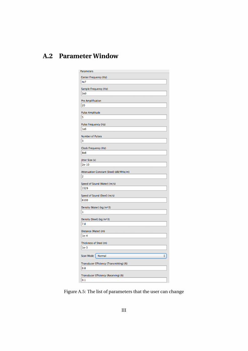
A.2 Parameter Window

Figure A.5: The list of parameters that the user can change

III

A.3 Normal Scan

Figure A.6: Plot of the scan result when using normal scan

A.4 Xilinx ISE and MATLAB related pulse generationfigures

The figures shows the generated pulse train in both MATLAB and Xilinx ISE. Inthe figures there is a small error because of the different sample clocks used inthe simulations. The Xilinx ISE figures represents the pulse train in 17 bits.

Figure A.7: The generated 17 bits pulse train, Xilinx ISE

IV

Figure A.8: The generated pulse train, MATLAB

Figure A.9: The zoomed in second pulse in the generated 17 bits pulse train,Xilinx ISE

V

Figure A.10: The zoomed in second pulse in the generated pulse train, MATLAB

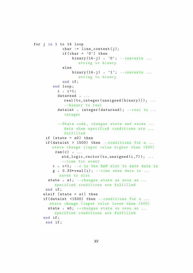
A.5 Signal processing Xilinx ISE

The figure shows signal processing for the first pulse response from the Simulinkoutput. When the 14 bits value converted to integer is considered as a peak thetime of arrival for the peak is saved to RAM.

Figure A.11: The signal processing for the 14 bits pulse respons in the interval0ns to 1140ns in Xilinx ISE, saves to RAM when the value converted to integeris higher than 1500

VI

B. CODE

B.1 Matlab

function [y] = pulse(c_freq, amp, samp_freq, pulse_freq, ...num_pulses)

%UNTITLED Summary of this function goes here% Detailed explanation goes here

if c_freq*2≤samp_freq && pulse_freq≤c_freq%Setting sample frequency and center frequencyfs=samp_freq;fc=c_freq;%Time vectort=linspace(−0.5/fc,0.5/fc,fs/fc);%Adjusts the shape of the pulses=0.15;a=fc*t/s;%Normalizes the pulse to an amplitude of 1norm=1/(exp(−1/2)/sqrt(2));%Creating the pulseyp=amp*norm*a.*exp(−a.^2);%Create the space between pulsesspace=zeros(1,(1/pulse_freq−1/fc)*fs−1);%Create a time vector corresponding to the pulse ...

frequency and the%number of pulsestime=linspace(0, ...

num_pulses*(1/pulse_freq),num_pulses*(length(yp)+length(space)));%Create the pulse trainy=[];for i=1:num_pulses

y=[y yp space];end

%Matched filter%b=yp(end:−1:1)/amp;

%Plot the pulses in time%plot(time,y)

%Plot filtered signal

VII

%fil=filter(b,1,y);%plot(time,fil)

end

y = pulse(fc,amp,fs,pf,np); %fc=center frequency, ...amp=amplitude, fs=sample frequency, pf=pulse frequency, ...np=nr of pulses

vec_lsb = 2^(−6); %vec_int = round( y / vec_lsb ); %converts the decimal values ...

to integers where vec_lsb determines the accuracy

fid = fopen('3.txt','wt'); %3.txt is the file, wt for ...writing in text mode

fprintf(fid,'%4.0f\n',vec_int); %Writes vec_int as one ...integer per row.

fclose(fid); %closes the file

function y = vga(u,t,first_delay,tot_delay,pulse_frequency)

time=mod(t−first_delay,1/pulse_frequency); %Calculates where ...in the period the signal is

if t≤first_delay %Only amplify if the first pulse resonce ...has arrivedy=u;

elseif time>tot_delay %Does not amplify if the the signal is ...after the third pulse responce and before the first ...responce of the next pulsey=u;

elsegain=16*time/tot_delay; %Amplifies linear to timey=u*gain;

end

VIII

function y1 = ...mathed_filter(u,b,sc,t,first_delay,tot_delay,pulse_frequency)

%Reverses the filter if it's the first pulse responseif mod(t−first_delay,pulse_frequency)≤first_delay

b=−1*b;end%Filters the signal, u is as many samples as the pulse itself.y = filter(b,1,u);y1=y(end); %Only put out the last element.

%Settings for the scantype. A−Scan will calculated the ...energy while Normal

%will display the signal as it is.switch sc

case 1%Normaly1=y(end);

case 2%A−Scannorm=1/sum(b.^2);y1=abs(y(end)*norm);

end

function Dataout = getBits()

A = textread('2.txt', '%s'); %Select file to readncols = size(A, 1); %Calculates number of columns in the A ...

matrixnrows = size(A{1}, 2); %Calculates number of rows in the A ...

matrixA = reshape(sscanf([A{:}], '%1d'), nrows, ncols); % Reshapes ...

A to a readable matrixDataout=A';

function y = saveToFile(hey)

fid = fopen('1.txt','wt'); % Opens file to write to and ...note the 'wt' for writing in text mode

% Put outs the data in a format that is readable in VHDL

IX

fprintf(fid,'%1.0f %1.0f %1.0f %1.0f %1.0f %1.0f %1.0f %1.0f ...%1.0f %1.0f %1.0f %1.0f %1.0f %.0f\n', hey');

fclose(fid);

X

B.2 VHDL

library std;use std.textio.all; --include package textio.vhdlibrary IEEE;use IEEE.STD_LOGIC_1164.ALL;use ieee.numeric_std.all;use ieee.std_logic_unsigned.all;use IEEE.std_logic_textio.all;

--entity declarationentity filehandle isend filehandle;

--architecture definitionarchitecture Behavioral of filehandle is

--period of clock ,bit for indicating end of file.signal clock ,end offile : bit := '0';

--type for the data to write.signal dataread : std_logic_vector (16 downto 0);

signal datatosave : real;

--line number of the file read or written.signal linenumber : integer :=1;

begin

clock ≤ not (clock) after 0.167 ns; --clock ...

with time period 0.334 ns(sample time)

--read processreading :process

XI

file infile : text is in "3.txt"; ...

--declare input filevariable inline : line; --line number ...

declarationvariable dataread1 : real;

beginwait until clock = '1' and clock 'event;if (not endfile(infile)) then --checking the ...

"END OF FILE" is not reached.readline(infile , inline); --reading a line ...

from the file.

read(inline , dataread1);dataread ≤...

std_logic_vector(to_signed(integer(dataread1) ,17)); ...

--converts the data to binaryelseendoffile ≤ '1'; --set signal to tell end ...

of file read file is reached.end if;

end process reading;

--write processwriting :process

file outfile : text is out "2. txt"; ...

--declare output filevariable outline : line; --line number ...

declarationbeginwait until clock = '0' and clock 'event;if(endoffile ='0') then --if the file end is not ...

reached.--write(linenumber ,value(binary ...

type),justified(side),field(width),digits(natural));write(outline , dataread , right , 17);-- write line to external file.writeline(outfile , outline);linenumber ≤ linenumber + 1; --jumps to next lineelse

XII

null;end if;

end process writing;

end Behavioral;

library std;use std.textio.all;library IEEE;use IEEE.STD_LOGIC_1164.ALL;use ieee.numeric_std.all;use ieee.std_logic_unsigned.all;use IEEE.std_logic_textio.all;

entity saveram is

end saveram;

architecture Behavioral of saveram is

type ram_t is array (0 to 255) of ...

std_logic_vector (6 downto 0); --256 slots ram , ...

7bits eachsignal ram : ram_t := (others => (others => '0'));signal c : integer range 0 to 255:=0; --index for ...

slot in RAM.signal i : integer range 0 to 10000:=0; ...

--minimum: nr of samplessignal g : real;

--period of clock ,bit for indicating end of file.signal endoffile : bit := '0';

--data read from the file.signal dataread : real;

XIII

--type of data from the input file.signal binary : std_logic_vector (13 downto ...

0) :="00000000000000"; --size of file to read

signal datatosave : integer;

signal dataint : integer range -10000 to ...

10000:=0;--line number of the file read or written.signal linenumber : integer :=1;

type state_type is (s0,s1);

signal state: state_type :=s0;

begin

--read processreading :process

variable line_content : string (1 to 14); ...

--size of file to readvariable line_num : line;variable j : integer := 0;

variable char : character :='0';file infile : text;

begin

file_open(infile ,"1. txt",READ_MODE); --declare ...

input filewhile not endfile(infile) loop --loop as long as ...

not the end of the filereadline (infile ,line_num); --line to read in fileREAD (line_num ,line_content);

XIV

for j in 1 to 14 loopchar := line_content(j);if(char = '0') then

binary (14-j) ≤ '0'; --converts ...

string to binaryelse

binary (14-j) ≤ '1'; --converts ...

string to binaryend if;

end loop;i ≤ i+1;dataread ≤ ...

real(to_integer(unsigned(binary))); ...

--binary to realdataint ≤ integer(dataread); --real to ...

integer

--State code , changes state and saves ...

data when specified conditions are ...

fulfilledif (state = s0) thenif(dataint > 1500) then --conditions for a ...

state change (input value higher than 1500)ram(c) ≤ ...

std_logic_vector(to_unsigned(i,7)); ...

--time for eventc ≤ c+1; --c is the RAM slot to save data ing ≤ 0.33* real(i); --time when data is ...

saved to slotstate ≤ s1; --changes state as soon as ...

specified conditions are fulfilledend if;

elsif (state = s1) thenif(dataint <1500) then --conditions for a ...

state change (input value lower than 1500)state ≤ s0; --changes state as soon as ...

specified conditions are fulfilledend if;end if;

XV

wait for 0.33 ns; --after reading each ...

line wait for 0.33ns(sample time).end loop;endoffile ≤ '1'; --sets endoffile =1 when ...

all the lines in the file are readfile_close(infile); --after reading all ...

the lines close the filewait;

end process;end Behavioral;

XVI