simulation, control and sensitivity analysis of crude oil distillation unit

Journal of Petroleum and Gas Engineering Vol. 3(6), pp. 99-113, November 2012 Available online at http://www.academicjournals.org/JPGE DOI: 10.5897/JPGE11.056 ISSN 2141-2677 ©2012 Academic Journals

Full Length Research Paper

Simulation, control and sensitivity analysis of crude oil distillation unit

Akbar Mohammadi Doust, Farhad Shahraki and Jafar Sadeghi*

Department of Chemical Engineering, Faculty of Engineering, University of Sistan and Baluchestan, Zahedan, Iran.

Accepted 23 April, 2012

Steady-state and dynamic simulation play important roles in investigation of refinery units. Therefore, simulation can help this investigation and behavior assessment. In this paper, simulation was done by commercial software. In fact, because of solving many state equations simultaneously and using control theory, dynamic simulation has more significant impact than steady-state simulation. Flow, pressure, temperature and level (FPTL) were controlled by Proportional-Integral-Derivative (PID) controllers in the unit. The case study is Kermanshah Refinery. The behavior of the FPTL controllers in dynamic regime were observed after the changing of the crude oil feed flow rate by 3% for 5 h. ASTM D86 boiling points (compositions) of two simulations were compared with experimental data. Finally, system sensitivity to inputs variables was investigated in the MATLAB®/Simulink

TM by transferring the

dynamic results. Transient responses to changes such as feed temperature, feed flow rates, steam flow rates and the duties of the reboilers of columns in Gasoline unit were plotted. Among of all disturbances, the system is more sensitive to changes in the feed temperature, the duties of the reboilers of columns in gasoline unit and simultaneous combination of above changes. Key words: Steady-state, dynamic, PID controller, ASTM D86, Sensitivity, MATLAB simulink, transition responses.

INTRODUCTION Today, distillation of crude oil is an important process in almost all of the refineries. Simulation of the process and analysis of the resulting data in both steady-state and dynamic conditions are fundamental steps in decreasing of the energy costs and controlling the quality of the oil products. The dynamic simulation when adding some Proportional-Integral-Derivative (PID) controllers and setting them to have desired responses, has more significant impacts and challenges than steady-state simulation in crude oil distillation units. A PID controller is a controller that includes three elements (Araki, 2002). PID control systems have exactly the same structure as depicted in Figure 1, where the PID controller is used as *Corresponding author. E-mail: [email protected]. Tel: +989155494265.

the compensator C(s). The transfer function of a PID controller is:

1( ) 1P D

I

C s K ss

ττ

= + +

(1)

All the three elements are kept in action. Here, PK ,

Iτ and Dτ are positive parameters, which are

respectively referred to as proportional gain, integral time, and derivative time, and as a whole, as PID parameters. These parameters can be adjusted using some empirical methods. One of them, which is an extension to Ziegler-Nichols method and uses the ultimate gain and frequency for adjustment of the parameters, is Tyreus-Luyben method (Almudena, 2001).

100 J. Petroleum Gas Eng.

Figure 1. Conventional feedback control system.

Crude oil is a mixture of many thousands of components varying from light hydrocarbons such as methane, ethane, propane, etc., to very high molecular weight components. The compositions of crude oil depend also on the location of exploitation. In the present work, the feed flow rate is 0.046 m

3/s (25,000 bbl/day)

that is provided by the blending of Crude oils of Ahwaz (60%), Naft-I-Shah (24%) and Maleh-Kuh (16%). Therefore, the feed has very complex compositions. Also the design and optimization of the oil fractionators are very important and complex. In petroleum refining the boiling point ranges are used instead of mass or mole fractions. Four types of boiling point analysis are known: ASTM D86, ASTM D1160, ASTM D158 and TBP (True Boiling Point). Six streams of product were investigated by ASTM D86 from initial boiling point (IBP) to final boiling point (FBP). We studied the system behavior by changing the feed flow rate in the dynamic conditions and MATLAB®/Simulink

TM. MATLAB software is very flexible

for this work, therefore, it was used. The aims of this work are to investigate the results in

steady-state and dynamic simulations, FPTL control while changing the crude oil feed flow rate and comparison of ASTM D86 boiling points (compositions) in two simulations with the correspondent experimental data. At last, sensitivity analysis of crude oil distillation unit in the MATLAB®/Simulink

TM was done by transferring dynamic

files to it as the basis aim. Directions of transferring files to sensitivity analysis were: Steady state files Dynamic files MATLAB®/Simulink

TM

Physical-mathematical model of the distillation column In the problems of multiple-stage separation for systems in which different phases and different components play a

part, we have to resort to the simultaneous or iterative solution of hundreds of equations. This means that it is necessary to specify a sufficient number of design variables so that the number of unknown quantities (output variables) is exactly the same as the number of equations (independent variables). This number of equation can be found and counted in a mathematical model.

The usual method to mathematically model a distillation process in refining columns is the theoretical stage method. To find the number of the theoretical stages of an existing column, the real number of stages might be multiplied by column efficiency. For each theoretical stage, the mass balance of individual components or pseudo components, energy balance, and vapor-liquid equilibrium equation can be written. The set of these equations creates the mathematical model of a theoretical stage. The mathematical model of a column is composed with models of individual theoretical stages. Finally, thermodynamic model Braun K10 “BK10” was used for the unit, because it is a model suitable for mixtures of heavier hydrocarbons at pressures under 700 kPa and temperatures from 170 to 430°C. The values of K10 can then be obtained by the Braun convergence pressure method using tabulated parameters for 70 hydrocarbons and light gases (Aspen Physical Property System, 2009). At low pressures, the Braun K10 model is strictly applicable to predict the properties of heavy hydrocarbon systems. Using the Braun convergence pressure method by the model at, given the normal boiling point of a component, K value is calculated at system temperature and 10 psia. The K10 value is then corrected for pressure using pressure correction charts. Using the modified Antoine equation one can find the K values for any components that are not covered by the charts at 10 psia and corrected to system conditions using the pressure correction charts (Aspen Physical Property System, 2009).

In existence of a large amount of acid gases or light

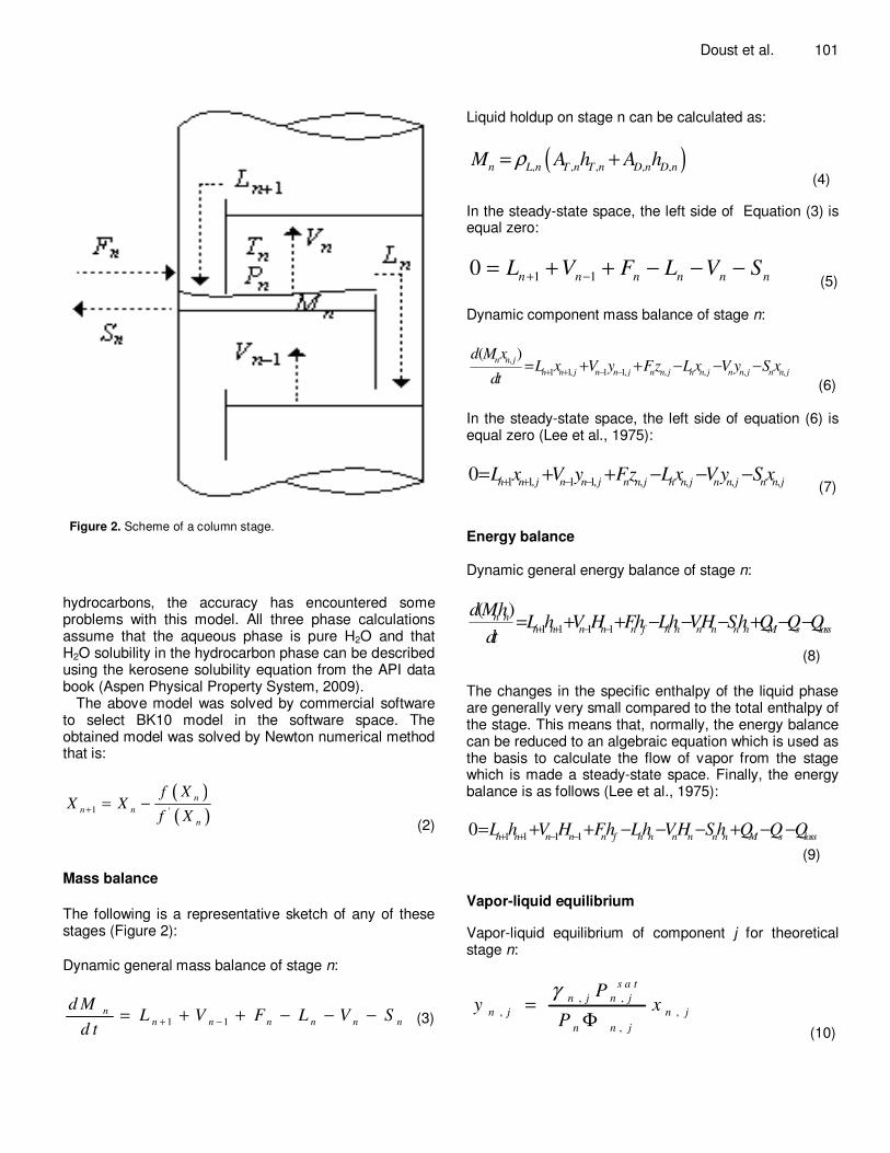
Figure 2. Scheme of a column stage.

hydrocarbons, the accuracy has encountered some problems with this model. All three phase calculations assume that the aqueous phase is pure H2O and that H2O solubility in the hydrocarbon phase can be described using the kerosene solubility equation from the API data book (Aspen Physical Property System, 2009).

The above model was solved by commercial software to select BK10 model in the software space. The obtained model was solved by Newton numerical method that is:

( )

( )1 '

n

n n

n

f XX X

f X+ = −

(2)

Mass balance

The following is a representative sketch of any of these stages (Figure 2):

Dynamic general mass balance of stage n:

1 1

nn n n n n n

d ML V F L V S

d t+ −= + + − − − (3)

Doust et al. 101 Liquid holdup on stage n can be calculated as:

( ), , , , ,n L n T n T n D n D nM A h A hρ= +

(4)

In the steady-state space, the left side of Equation (3) is equal zero:

1 10

n n n n n nL V F L V S

+ −= + + − − −

(5)

Dynamic component mass balance of stage n:

,

1 1, 1 1, , , , ,

( )n n j

n n j n n j n n j n n j n n j n n j

d M xL x V y Fz L x V y S x

dt+ + − −= + + − − −

(6) In the steady-state space, the left side of equation (6) is equal zero (Lee et al., 1975):

1 1, 1 1, , , , ,0

n n j n n j n n j n n j n n j n n jL x V y Fz Lx V y S x+ + − −= + + − − −

(7) Energy balance Dynamic general energy balance of stage n:

1 1 1 1

( )n nn n n n n f n n n n n n M s loss

d MhL h V H Fh Lh VH Sh Q Q Q

dt+ + − −= + + − − − + − −

(8)

The changes in the specific enthalpy of the liquid phase are generally very small compared to the total enthalpy of the stage. This means that, normally, the energy balance can be reduced to an algebraic equation which is used as the basis to calculate the flow of vapor from the stage which is made a steady-state space. Finally, the energy balance is as follows (Lee et al., 1975):

1 1 1 10

n n n n n f n n n n n n M s lossL h V H Fh Lh VH S h Q Q Q

+ + − −= + + − − − + − −

(9)

Vapor-liquid equilibrium

Vapor-liquid equilibrium of component j for theoretical stage n:

, ,

, ,

,

s a t

n j n j

n j n j

n n j

Py x

P

γ=

Φ (10)

102 J. Petroleum Gas Eng. Table 1. The Mass flows of the atmospheric column products.

Product Mass flow (Kg/s)

Naphtha 19.43

Blending naphtha 0.25

Kerosene 6.55

Atmosphere gas oil 6.38

Atmospheric residue 15.68

Table 2. The Mass flows of the debutanizer column products.


To fuel 0.38

To LPG unit 0.72

Bottom product 8.2

Table 3. The Mass flows of the splitter column products.


To flare 0.01

To LSRG Merox 2.1

HSRG to platforming 6.1

This equation is the equilibrium and in real state. If each

of vapor or liquid phase is ideal then ,n j

Φ or ,n j

γ is unit,

respectively. If both phases are ideal then ,n j

Φ and ,n j

γ

are unit. Therefore, the above equation is converted to Raoult’s equation:

, , ,

sat

n j n n j n jy P x P= (11)

Pressure

1n nP P P+= + ∆

(12)

2

0V

PK

∆ =

(13)

Where 0

V the volumetric flow is rate of live stream in

m3/h and K is the proportionality constant in m

3/bar

0.5.h.

The value of K for each geometry is different and has specific value which is chosen by software (Almudena, 2001; Lee et al., 1975).

Steady-state simulation In this work, distillation unit of Kermanshah Refinery was simulated. The three assays of crude oil were characterized by the TBP (True Boiling Point) data, API gravity and light components.

The unit consists of 5 heat exchangers, 2 coolers, 2 heaters, atmospheric column, debutanizer column, splitter column, valves and pumps. The atmospheric column as the main part of the unit had three side strippers and two pumparounds. Important parameters for the pumparound specification are the drown off and the return stages, mass flow rate and temperature drop. For the side strippers, beside the product flow rate, the specification of the steam flow and parameters, the drown off and the return stages, and the number of stripper stages were entered. The feed flow rate of 0.046 m

3/s (25,000 bbl/day) of crude oil was preheated. Then, it

was entered to the 35th stage of the atmospheric column

with 38 theoretical stages. Temperature of the feed was 328.11°C (622.6°F). Products of the column are naphtha, blending naphtha, kerosene, atmospheric gas oil and atmospheric residue. Table 1 shows their mass flow rates.

The product of kerosene, atmospheric gas oil and atmospheric residue played an important role in preheating of the feed, because they had high temperatures, hence energy optimization was done.

To purify the naphtha, firstly it was cooled to 26.67°C (80°C). Then the naphtha stream was entered to a two-phase separator and splitter. Fifty percent of the flow was returned as the reflux stream and the other half was preheated and entered to the debutanizer column. The bottom product preheated the feed and entered to splitter column.

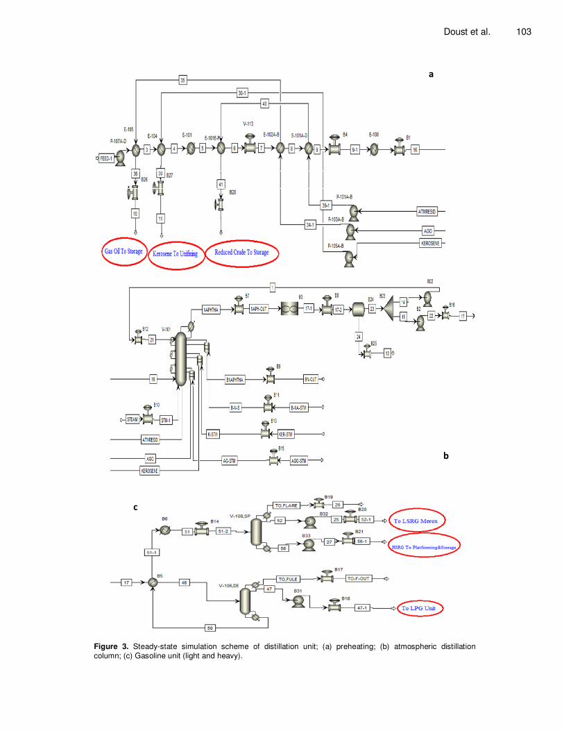
Tables 2 and 3 show the mass flow rates of the products (Tables 2 and 3). Also, Figure 3 illustrates the steady-state simulation scheme of the above steps in continuous forms.

Dynamic simulation

After steady-state simulation to observation the effects of changes the crude oil feed in the products of unit and investigation of results in real processes, we exported the stead-state simulation to dynamic simulation.

Before transferring the steady-state files, dynamic simulation requirements should be entered. In addition, the pressure changers (valves, pumps, etc.) are necessary and sensitive to exporting of steady-state simulation to dynamic simulation by “export dynamic (pressure driven)”.

For example dynamic requirements of column are column diameter, tray spacing, tray active area, weir

Doust et al. 103

a

b

c

Figure 3. Steady-state simulation scheme of distillation unit; (a) preheating; (b) atmospheric distillation

column; (c) Gasoline unit (light and heavy).

104 J. Petroleum Gas Eng. length, weir height, reflux drum length and diameter, and sump length and diameter. A “tray sizing” tool can be used to calculate the tray sizes based on flow conditions in the column. Of course, all of dynamic simulation requirements were provided by Research and Development (R&D) Bureau of Kermanshah Refinery.

After entering data and exporting to dynamic simulation in order to control the flow, pressure, temperature and level of streams, especially all products than changing of crude oil feed, controllers should be added in right places in the dynamic space. Dynamic space provides a number of different types of controllers. The PID Incr. model was used for all controllers in the dynamic space. The parameters of each controller (gain, integral time and derivative time) were set to optimal values using the assistance of the “tuning” tool and Tyreus-Luyben method (Luyben, 2006; Juma and Tomáš, 2009). Figure 4 illustrates the dynamic simulation scheme of continuous forms (Figure 4). Streams ID are corresponding to the steady-state simulation scheme. RESULTS AND DISCUSSION Distillation temperature ASTM D86 After changing the crude oil feed flow rate, ASTM D86 of six streams ((“52-1”, light gasoline), (“56-1”, heavy gasoline), the feed of debutanizer column (V-106, DE), blending naphtha, kerosene and atmospheric gas oil) in three spaces of experimental, steady-state and dynamic were compared. Experimental data were provided by R&D Bureau of Kermanshah Refinery.

Figures 5 to 10 show a comparison between the experimental ASTM D86 curves with the results of the steady-state and the dynamic simulations. Curves of the feed of debutanizer column (V-106, DE) and atmospheric gas oil stream were in better agreement with the experimental data than the other streams. Of course, maximum difference of other streams was around 12°C. Totally, results of simulations were in good agreement with the experimental data (Kermanshah Refinery, 2009). 2- Sensitivity analysis in the MATLAB simulink The behaviors of the FPTL controllers in dynamic simulation were observed by increasing the crude oil feed flow rate (+3%). The FPTL were controlled by conventional PID controllers. Set points were set based on Kermanshah Refinery. Twenty-three controllers were applied to control of FPTL of the unit. We tried to set the controller parameters and solved of fluctuations by different control methods to reach a new steady-state. To set the controller parameters, Tyreus-Luyben method

was employed. At last, we investigated of dynamic results by transferring the dynamic files to MATLAB®/Simulink

TM

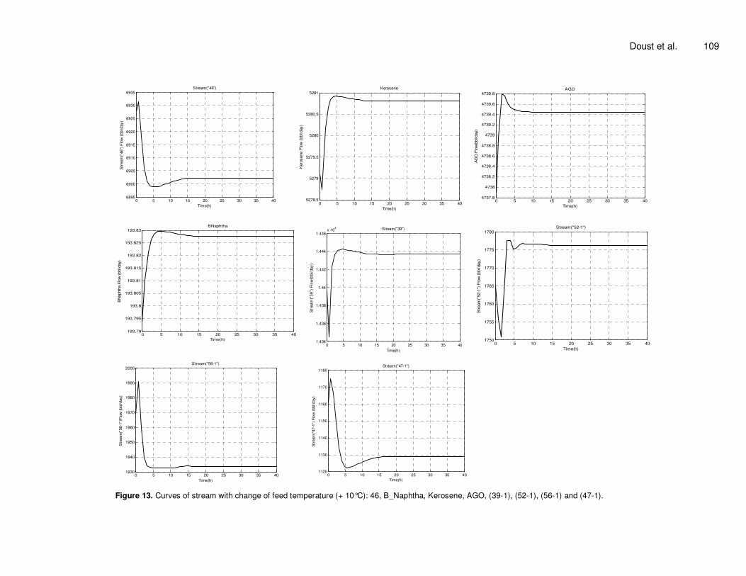
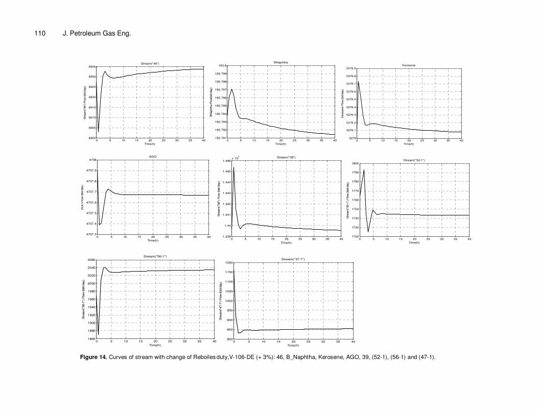
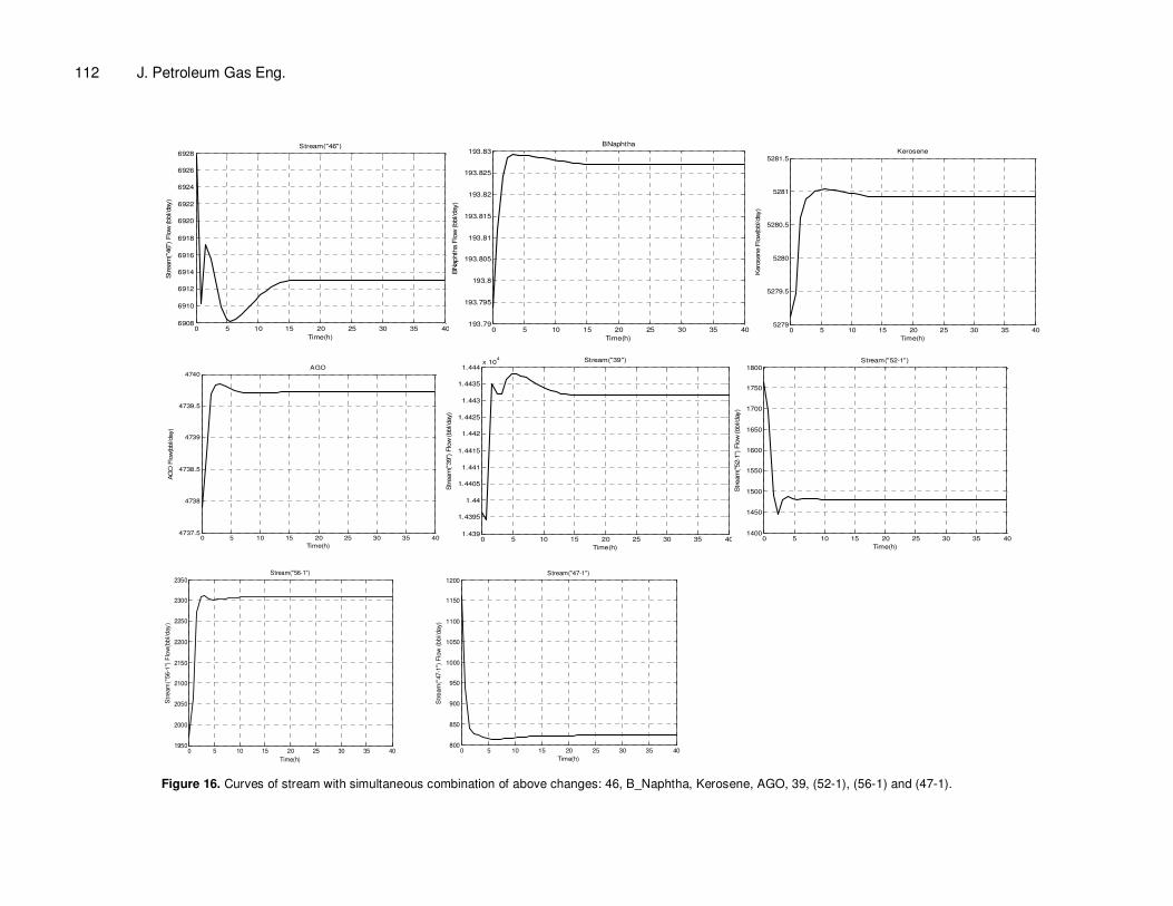
Figure 11. The first steady-state then system sensitivity was observed by step changes. Input variables were: 1. Feed temperature (+10°C). 2. Feed flow rates: Ahwaz (+1%), Maleh-Kuh (+1%), Naft-I-Shah (+1%) 3. Steam flow rates: STEAM (interring to atmospheric column, +20%), blending naphtha, steam (+50%), kerosene steam (+30%), atmospheric gas oil (AGO) steam (+30%). 4. The duty of Reboilers: debutanizer column (V-106-DE, +3%), splitter column (V-108- SP, +3%). 5. Mixed of above changes simultaneously. And outputs were: Stream flow rates: “46” (interring to V-106-DE), blending naphtha, kerosene, atmospheric gas oil (AGO), “39-1” (bottom of atmospheric column), “52-1” (light gasoline, up of V-108-SP column), “56-1” (heavy gasoline, bottom of V-108-SP column), “47-1” (to LPG unit). Because we wanted to increase the products, increasing of inputs were investigated. After performing above changes, we observed that the major sensitivity was related to feed temperature, the duties of the reboilers of columns in gasoline unit and simultaneous combination of above changes (Figures 12-16). Rest of input changes was not significant to steady-state. Conclusions Steady-state and dynamic simulations performed a good investigation into the process and discussing the calculated results. Control of variables in dynamic simulation as a flexible simulator like a pilot, was done very well.

Steady-state and dynamic simulations were in agreement with the experimental data. Any Increment of crude oil feed flow rate, made a complex fluctuations in the FPTL controllers that must be rejected by set of controller parameters and different control methods. Because the feed was a mixture of 3 crude oils and many components, control of system was very complex. The dynamic space demonstrated that temperature controllers were faster and more sensitive than the other controllers. Control of temperature can be replaced by control of the product compositions. In this control structure, small control errors in the FPTL controllers were observed. Therefore, some limitations in dynamic simulation were observed. Because of more flexibility of changing the inputs, disturbances and easier handling of graphs, dynamic files results transferred to

Doust et al. 105

a

b

c

Figure 4. Dynamic simulation scheme of distillation unit; (a) preheating; (b) Atmospheric distillation column; (c) Gasoline unit (light and heavy).


0 20 40 60 80 100100

120

140

160

180

200

220

240

260

280

Amount distillated(%)

Dis

tilla

tion t

em

pera

ture

AS

TM

D86(F

)

Experimental

Steady-state

Dynamic

Figure 5. Steady-state, dynamic and experimental ASTM D86 curves of “52-1” stream.

0 20 40 60 80 100180

200

220

240

260

280

300

320

340


Dis

tilla

tio

n t

em

pe

ratu

re A

ST

M D

86

(F)

Experimental

Steady-state

Dynamic

Figure 6. Steady-state, dynamic and experimental ASTM D86

curves of “56-1” stream.

MATALB®/SimulinkTM

. Figures 12 to 16 show that more sensitive disturbances were feed temperature, the duties of the reboilers of columns in gasoline unit and simultaneous combination of above changes. Rest of input changes was not significant in transient responses. Therefore, above variables play important roles in the design of distillation units.

0 20 40 60 80 10050

100

150

200

250

300

350


Dis

tilla

tio

n t

em

pe

ratu

re A

ST

M D

86

(F)

Experimental

Steady-state

Dynamic

Figure 7. Steady-state, dynamic and experimental ASTM D86 curves of column feed (V-106, DE).

0 20 40 60 80 100260

280

300

320

340

360

380

400

420

440


Dis

tilla

tio

n t

em

pe

ratu

re A

ST

M D

86

(F)

Experimental

Steady-state

Dynamic

Figure 8. Steady-state, dynamic and experimental ASTM D86 curves of Blending Naphtha (B_NAPHTHA Stream).

ACKNOWLEDGMENT The financial support provided by the Kermanshah Oil Refining Company is gratefully acknowledged.

Doust et al. 107

0 20 40 60 80 100250

300

350

400

450

500

550

600


Distilla

tion temperature A

STM D

86(F

)

Experimental

Steady-State

Dynamic

Figure 9. Steady-state, dynamic and experimental ASTM D86 curves of Kerosene.

0 20 40 60 80 100400

450

500

550

600

650

700

750


Distilla

tion temperatu

re A

STM

D86(F

)

Experimental

Steady-state

Dynamic

Figure 10. Steady-state, dynamic and experimental ASTM D86 curves of atmospheric gas oil (AGO stream).

Figure 11. Scheme of Distillation unit in the MATLAB simulink with inputs and outputs.


0 5 10 15 20 25 30 35 404737.65

4737.7

4737.75

4737.8

4737.85

4737.9

Time(h)

AG

O F

low

(bbl/day)

AGO

0 5 10 15 20 25 30 35 401764

1764.5

1765

1765.5

1766

1766.5

1767

1767.5

Time(h)

Stream

("52-1

") F

low

(bbl/day)

Stream("52-1")

0 5 10 15 20 25 30 35 401.4395

1.4396

1.4397

1.4398

1.4399

1.44

1.4401

1.4402

1.4403x 10

4

Time(h)

Str

eam

("39")

Flo

w (

bbl/day)

Stream("39")

0 5 10 15 20 25 30 35 401962

1963

1964

1965

1966

1967

1968

1969

1970

Time(h)

Str

eam

("56-1

") F

low

(bbl/day)

Stream("56-1")

0 5 10 15 20 25 30 35 401153

1154

1155

1156

1157

1158

1159

1160

1161

Time(h)

Stream

("47-1

") F

low

(bbl/day)

Stream("47-1")

0 5 10 15 20 25 30 35 40193.791

193.7915

193.792

193.7925

193.793

193.7935

193.794

Time(h)

BN

aphth

a F

low

(bbl/day)

BNaphtha

0 5 10 15 20 25 30 35 405279.06

5279.08

5279.1

5279.12

5279.14

5279.16

5279.18

5279.2

5279.22

Time(h)

Kero

sene F

low

(bbl/day)

Kerosene

0 5 10 15 20 25 30 35 406921

6922

6923

6924

6925

6926

6927

6928

Time(h)

Stream

("46")

Flo

w (bbl/day)

Stream("46")

Figure 12. Steady-state curves of stream: 46, B_Naphtha, Kerosene, AGO, (39-1), (52-1), (56-1) and (47-1).

Doust et al. 109

0 5 10 15 20 25 30 35 406895

6900

6905

6910

6915

6920

6925

6930

6935

Time(h)

Str

eam

("46")

Flo

w (

bbl/day)

Stream("46")

0 5 10 15 20 25 30 35 404737.8

4738

4738.2

4738.4

4738.6

4738.8

4739

4739.2

4739.4

4739.6

4739.8

Time(h)

AG

O F

low

(bbl/day)

AGO

0 5 10 15 20 25 30 35 401750

1755

1760

1765

1770

1775

1780

Time(h)

Stream

("52-1

") F

low

(bbl/day)

Stream("52-1")

0 5 10 15 20 25 30 35 40193.79

193.795

193.8

193.805

193.81

193.815

193.82

193.825

193.83

Time(h)

BN

aphth

a F

low

(bbl/day)

BNaphtha

0 5 10 15 20 25 30 35 405278.5

5279

5279.5

5280

5280.5

5281

Time(h)

Kero

sene F

low

(bbl/day)

Kerosene

0 5 10 15 20 25 30 35 401.434

1.436

1.438

1.44

1.442

1.444

1.446x 10

4

Time(h)

Str

ea

m("

39

") F

low

(bb

l/da

y)

Stream("39")

0 5 10 15 20 25 30 35 401930

1940

1950

1960

1970

1980

1990

2000

Time(h)

Str

eam

("56-1

")F

low

(bbl/day)

Stream("56-1")

0 5 10 15 20 25 30 35 401120

1130

1140

1150

1160

1170

1180

Time(h)

Str

eam

("47

-1")

Flo

w (

bbl/d

ay)

Stream("47-1")

Figure 13. Curves of stream with change of feed temperature (+ 10°C): 46, B_Naphtha, Kerosene, AGO, (39-1), (52-1), (56-1) and (47-1).


0 5 10 15 20 25 30 35 406900

6905

6910

6915

6920

6925

6930

6935

Time(h)

Stream

("46")

Flo

w (bbl/day)

Stream("46")

0 5 10 15 20 25 30 35 40193.791

193.792

193.793

193.794

193.795

193.796

193.797

193.798

193.799

193.8

Time(h)

BNaphth

a F

low(b

bl/day)

BNaphtha

0 5 10 15 20 25 30 35 405279

5279.1

5279.2

5279.3

5279.4

5279.5

5279.6

5279.7

5279.8

5279.9

Time(h)

Kero

sene F

low

(bbl/day)

Kerosene

0 5 10 15 20 25 30 35 404737.3

4737.4

4737.5

4737.6

4737.7

4737.8

4737.9

4738

Time(h)

AG

O F

low

(bbl/day)

AGO

0 5 10 15 20 25 30 35 401.439

1.44

1.441

1.442

1.443

1.444

1.445

1.446x 10

4

Time(h)

Stream

("39")

Flo

w (bbl/day)

Stream("39")

0 5 10 15 20 25 30 35 401720

1730

1740

1750

1760

1770

1780

1790

1800

Time(h)

Stream

("52-1

") F

low

(bbl/day)

Stream("52-1")

0 5 10 15 20 25 30 35 401860

1880

1900

1920

1940

1960

1980

2000

2020

2040

2060

Time(h)

Stream

("56-1

") F

low

(bbl/day)

Stream("56-1")

0 5 10 15 20 25 30 35 40800

850

900

950

1000

1050

1100

1150

1200

Time(h)

Stream

("47-1

") F

low (bbl/day)

Stream("47-1")

Figure 14. Curves of stream with change of Reboiles

’duty,V-106-DE (+ 3%): 46, B_Naphtha, Kerosene, AGO, 39, (52-1), (56-1) and (47-1).

Doust et al. 111

0 5 10 15 20 25 30 35 406921

6922

6923

6924

6925

6926

6927

6928

Time(h)

Str

eam

("4

6")

Flo

w (

bbl/d

ay)

Stream("46")

0 5 10 15 20 25 30 35 40193.791

193.7915

193.792

193.7925

193.793

193.7935

193.794

Time(h)

BN

aphth

a F

low

(bbl/day)

BNaphtha

0 5 10 15 20 25 30 35 405279.06

5279.08

5279.1

5279.12

5279.14

5279.16

5279.18

5279.2

5279.22

Time(h)

Kero

sene F

low

(bbl/day)

Kerosene

0 5 10 15 20 25 30 35 404737.65

4737.7

4737.75

4737.8

4737.85

4737.9

Time(h)

AG

O F

low

(bbl/day)

AGO

0 5 10 15 20 25 30 35 401.4395

1.4396

1.4397

1.4398

1.4399

1.44

1.4401

1.4402

1.4403x 10

4

Time(h)

Str

eam

("39")

Flo

w (

bbl/day)

Stream("39")

0 5 10 15 20 25 30 35 401450

1500

1550

1600

1650

1700

1750

1800

Time(h)

Str

eam

("52-1

") F

low

(bbl/day)

Stream("52-1")

0 5 10 15 20 25 30 35 401950

2000

2050

2100

2150

2200

2250

2300

Time(h)

Str

ea

m("

56-1

') F

low

(bbl/day)

Stream("56-1")

0 5 10 15 20 25 30 35 401153

1154

1155

1156

1157

1158

1159

1160

1161

Time(h)

Str

eam

("47-1

") F

low

(bbl/day)

Stream("47-1")

Figure 15. Curves of stream with change of Reboiles

’duty,V-108-SP (+ 3%): 46, B_Naphtha, Kerosene, AGO, 39 , (52-1), (56-1) and (47-1).


0 5 10 15 20 25 30 35 406908

6910

6912

6914

6916

6918

6920

6922

6924

6926

6928

Time(h)

Stream

("46")

Flo

w (bbl/day)

Stream("46")

0 5 10 15 20 25 30 35 40193.79

193.795

193.8

193.805

193.81

193.815

193.82

193.825

193.83

Time(h)

BN

aphth

a F

low

(bbl/day)

BNaphtha

0 5 10 15 20 25 30 35 405279

5279.5

5280

5280.5

5281

5281.5

Time(h)

Kero

sene F

low

(bbl/day)

Kerosene

0 5 10 15 20 25 30 35 404737.5

4738

4738.5

4739

4739.5

4740

Time(h)

AG

O F

low

(bbl/day)

AGO

0 5 10 15 20 25 30 35 401.439

1.4395

1.44

1.4405

1.441

1.4415

1.442

1.4425

1.443

1.4435

1.444x 10

4

Time(h)

Stream

("39")

Flo

w (bbl/day)

Stream("39")

0 5 10 15 20 25 30 35 401400

1450

1500

1550

1600

1650

1700

1750

1800

Time(h)

Stream

("52-1

") F

low

(bbl/day)

Stream("52-1")

0 5 10 15 20 25 30 35 401950

2000

2050

2100

2150

2200

2250

2300

2350

Time(h)

Str

eam

("56

-1")

Flo

w(b

bl/d

ay

)

Stream("56-1")

0 5 10 15 20 25 30 35 40800

850

900

950

1000

1050

1100

1150

1200

Time(h)

Stream

("47-1

") F

low

(bbl/day)

Stream("47-1")

Figure 16. Curves of stream with simultaneous combination of above changes: 46, B_Naphtha, Kerosene, AGO, 39, (52-1), (56-1) and (47-1).

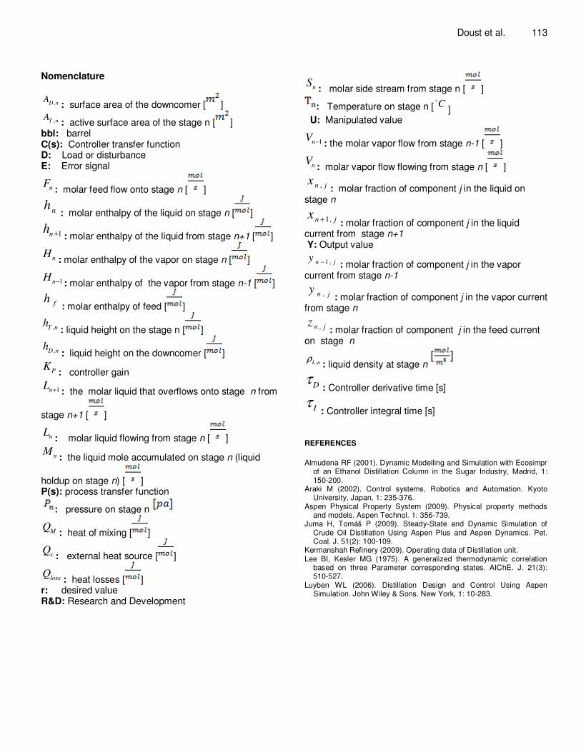
Nomenclature

,D nA: surface area of the downcomer [ ]

,T nA: active surface area of the stage n [ ]

bbl:

barrel

C(s): Controller transfer function D: Load or disturbance E: Error signal

nF

: molar feed flow onto stage n [ ]

nh

: molar enthalpy of the liquid on stage n [ ]

1nh + : molar enthalpy of the liquid from stage n+1 [ ]

nH

: molar enthalpy of the vapor on stage n [ ]

1nH − : molar enthalpy of the vapor from stage n-1 [ ]

fh: molar enthalpy of feed [ ]

,T nh

: liquid height on the stage n [ ]

,D nh

: liquid height on the downcomer [ ]

PK

: controller gain

1nL + : the molar liquid that overflows onto stage n from

stage n+1 [ ]

nL

: molar liquid flowing from stage n [ ]

nM

: the liquid mole accumulated on stage n (liquid

holdup on stage n) [ ] P(s): process transfer function

: pressure on stage n

MQ

: heat of mixing [ ]

sQ

: external heat source [ ]

lossQ

: heat losses [ ] r: desired value R&D: Research and Development

Doust et al. 113

nS

: molar side stream from stage n [ ]

: Temperature on stage n [ Co]

U: Manipulated value

1nV − : the molar vapor flow from stage n-1 [ ]

nV

: molar vapor flow flowing from stage n [ ]

,n jx: molar fraction of component j in the liquid on

stage n

1,n jx + : molar fraction of component j in the liquid current from stage n+1 Y: Output value

1 ,n jy − : molar fraction of component j in the vapor

current from stage n-1

,n jy: molar fraction of component j in the vapor current

from stage n

,n jz: molar fraction of component j in the feed current

on stage n

,L nρ: liquid density at stage n

Dτ: Controller derivative time [s]

Iτ: Controller integral time [s]

REFERENCES

Almudena RF (2001). Dynamic Modelling and Simulation with Ecosimpr

of an Ethanol Distillation Column in the Sugar Industry, Madrid, 1: 150-200.

Araki M (2002). Control systems, Robotics and Automation. Kyoto University, Japan, 1: 235-376.

Aspen Physical Property System (2009). Physical property methods and models. Aspen Technol. 1: 356-739.

Juma H, Tomáš P (2009). Steady-State and Dynamic Simulation of Crude Oil Distillation Using Aspen Plus and Aspen Dynamics. Pet. Coal. J. 51(2): 100-109.

Kermanshah Refinery (2009). Operating data of Distillation unit. Lee BI, Kesler MG (1975). A generalized thermodynamic correlation

based on three Parameter corresponding states. AIChE. J. 21(3): 510-527.

Luyben WL (2006). Distillation Design and Control Using Aspen Simulation. John Wiley & Sons. New York, 1: 10-283.

simulation, control and sensitivity analysis of crude oil distillation unit

Documents