simulation and control of complex a dissertation …
TRANSCRIPT

SIMULATION AND CONTROL OF COMPLEX
DISTILLATION PROCESSES
by
HAITAO HUANG, B.E., M.S.Ch.E.
A DISSERTATION
IN
CHEMICAL ENGINEERING
Submitted to the Graduate Faculty of Texas Tech University in
Partial Fulfillment of the Requirements for
the Degree of
DOCTOR OF PHILOSOPHY
Approved
May, 2000
Copyright 2000, Haitao Huang

ACKNOWLEDGEMENTS
I would like to thank Dr. James B. Riggs, my advisor, for his help and support
over the last three years, and for giving me the opportunity to join his research group and
study under his supervision. I would also like to thank my committee members. Dr. D.
Bagert, Dr. R. Tock, and Dr. T. Weisner, for their help and patience throughout my study.
Without the help of Scott Boyden of Aspen Technology, Inc., in Houston, this
work would be impossible. I deeply appreciate his input of process knowledge,
generosity in spending time with me from his busy schedule, and his guidance on
DMCPlus^"^ applications in this study. I would also like to thank Dr. Charles R. Cutler
for his help on the main fractionator project, and for his guidance and valuable
suggestions.
I would like to acknowledge the help of my fellow graduate students, Marshall
Duvall, Joe Anderson, Scott Hurowitz, Xuan Li and J. Govindh. With their help,
difficulties and problems in my research project were overcome quickly.
Finally, I am indebted to my family members. 1 thank my wife, Xiaowu, for her
love and understanding; my parents-in-law for taking care of our son, Michael, and for
their understanding and support; and my parents for their continuous support and
encouragement.

TABLE OF CONTENTS
ACKNOWLEDGEMENTS ii
ABSTRACT v
LIST OF TABLES vii
LIST OF FIGURES ix
CHAPTER
1. INTRODUCTION 1
1.1 Main Fractionators 1
1.2 Series of Distillation Columns 3
1.3 Model Predictive Control 4
1.4 Objectives 6
1.5 Dissertation Outline 6
2. DYNAMIC MODEL OF AN FCCU MAIN FRACTIONATOR 7
2.1 Process Description 7
2.2 Steady State Design 8
2.3 Model Assumptions 13
2.4 Thermodynamic Model 14
2.4.1 Feed Characterization 14
2.4.2 VLE and Enthalpy Calculations 19
2.5 Energy £md Mass Balance 20
2.5.1 Trays 21
2.5.2 Condenser and Accumulator 22
2.5.3 HCN stripper Reboiler 22
2.5.4 Main Colunrn and LCO Stripper Bottom Sumps 23
2.6 Numerical Algorithm 23
3. MAIN FRACTIONATOR CONTROL 27
3.1 Decentralized Control 27
3.1.1 Configuration Selection 27
3.1.2 Level Controller Tuning 29
3.1.3 Open Loop Responses 30
ni

3.1.4 Decouplers 33
3.1.5 Tuning Controllers 35
3.2 DMCPlus™ Control 37
3.2.1 Controller Implementation 3 8
3.3 Results and Analysis 40
3.4 Discussion of Results 47
4. MODELING OF A GAS RECOVERY UNIT 48
4.1 Process Description 48
4.2 Model Development 54
4.2.1 Pressure Dynamics 54
4.2.2 Heat Exchanger Dynamics 55
4.2.3 Condenser Heat Transfer Dynamics 57
4.2.4 Pressure Drop 60
5. GRU CONTROL 62
5.1 Decentralized Control for GRU 62
5.1.1 Configuration Considerations for the Quality Controls 62
5.1.2 Constraint Handling 65
5.1.3 Inferential Control 67
5.1.4 Tuning PID Controllers 67
5.2 DMCPlus™ Control of GRU 70
5.2.1 Control Strategy Design 70
5.2.2 Tuning DMCPlus™ Controllers 72
5.2.3 Resuhs 76
5.3 Comparing the Decentralized Control and the DMCPlus'' ' control 81
5.4 Discussion of Results 92
6. CONCLUSIONS AND RECOMMENDATIONS 93
6.1 Conclusions 93
6.2 Recommendations 95
REFERENCES 97
IV

ABSTRACT
The proper choice and implementation of control method improve reliability and
performance of distillation column control, which can translate into a reduction of energy
usage while maintaining product quality and rates, hence economic benefit. However,
clear guidelines to determine which and when advanced control strategies should be used
instead of traditional control strategies are still not available. Previous work has been
focused on two-product single columns. In this study, two complex distillation processes,
a fluid catalytic cracker unit (FCCU) main fractionator and a gas recovery unit, are
simulated with rigorous models. Traditional decentralized and model predictive control
(MPC) are applied to both processes, and their performances are compared in terms of
their capability to handle constrained multivariable processes.
A detailed tray-to-tray rigorous model for the FCCU main fractionator is
developed, in which the Soave-Redlich-Kwong (SRK) equations are used to model
vapor-liquid phase equilibrium. The feed is characterized as a mixture of 36 pseudo-
components and 9 defined components including water, hydrogen and light hydrocarbons
from CI to C4. An efficient algorithm is developed to solve the dynamic model
equations. Two decentralized control systems, one without decoupler, one with a simple
decoupler are implemented, and compared with a DMCPlus^"^ controller. The
DMCPlus^"^ controller performs better than both decentralized controls due to its superior
decoupling power.
The gas recovery unit consists of three distillation columns operated in series with
feed-bottoms heat integration for the first column. Rigorous models are developed for the
columns and the heat exchanger, including pressure and heat transfer dynamics. The
process is a highly coupled system and has interactive constraints that exist in different
units. A decentralized control system with override controls for constraints is designed,
implemented on the GRU simulator, and is compared with a DMCPlus^"^ controller with
10 independent variables and 12 dependent variables. The DMCPlus'' ' controller
outperforms the decentralized control system in terms of constraint handling due to its
flexibility.

The effects of including level control into MPC are also investigated. Three
DMCPlus''"' controllers with different strategies for controlling the bottom level of the
first column are implemented for the GRU process. The first DMCPlus^"^ controller does
not control the level, while the second one moves setpoint to the PI level controller, and
the third one controls the level directly by manipulating the deethanizer bottoms flow.
The results show that including level into MPC controller improves composition control
in cases that the manipulated variable for the level control has significant impact on
compositions.
VI

LIST OF TABLES
2.1 Design specifications and parameters for the main fractionator 12
2.2 Feed TBP curve at 1 atm 15
2.3 Properties of pseudo-components 16
2.4 Feed Composition 18
3.1 A typical industrial MV and CV pairing for the main fractionator 28
3.2 Timing parameters for level controllers 29
3.3 Steady state gains 34
3.4 Tuning parameters for the PI controllers without decoupler applied to the main fractionator 37
3.5 Tuning parameters for the PI controllers with a simple decoupler applied to the main fractionator 37
3.6 Tuning parameters for CVs in the DMCPlus^"^ controller for the main fractionator 39
3.7 Tuning parameters for the MVs in the DMCPlus "* controller for the main
fractionator 39
3.8 lAEs for setpoint changes 41
3.9 lAEs for a heavier feed change 41
3.10 I AEs for a lighter feed change 41
4.1 Summary of stream properties for the GRU process 48
4.2 Design parameters for the GRU columns 51
5.1 Control point names used for GRU process control. 64
5.2 Configuration for GRU decentralized control. 65
5.3 Implementation of the four override confrols 66
5.4 Tray temperatures used to infer compositions. 67
5.5 Tuning parameters for pressure and level confroUers 68
5.6 Tuning parameters for temperature controllers 68
5.7 Tuning parameters for composition controllers 69
5.8 Tuning parameters for override controllers 69
5.9 Independent and dependent variables included in all three DMCPlus''"' controllers 72
5.10 MV tuning parameters for DMC-1 and DMC-2 74
vii
5.11 MV tuning parameters for DMC-3 74
5.12 CV tuning parameters for all three DMCPlus™ controllers 75
5.13 lAE reduction compared to DMCPlus"""" without level included 81
6.1 Comparison between decentralized and MPC control strategies 94
Vlll

LIST OF FIGURES
2.1. Main fractionator process diagram 9
2.2 Steady state temperature profile 10
2.3 Steady state liquid flow profile 10
2.4 Steady state vapor flow profile 11
2.5 Flows around stage i of the main fractionator 21
2.6 A single flash stage. 24
2.7 Diagram for major calculation steps in main fractionator simulation. 26
3.1 Responses to a 2% increase in Qpi 31
3.2 Responses to a 2% increase in HCN product flow Fpi. 31
3.3 Responses to a 20% increase in LCO reflux L22, 32
3.4 Responses to a 2% increase in Qpe. 32
3.5 Simple decoupler implementation 35
3.6 Responses to a heavier feed 42
3.7 Responses to a lighter feed. 44
4.1 Process diagram of the gas recovery unit 53
4.2 Heat exchanger 56
4.3 Depropanizer overhead section 59
5.1 DMCPlus''"' control composition responses to a heavier feed. 77
5.2 DMCPlus^"^ control Composition responses to a lighter feed. 79
5.3 Caomparing DMCPlus^"^ and PI composition responses to a heavier feed 82
5.4 Responses of constraint and economical variables to a heavier feed. 84
5.5 Caomparing DMCPlus''"' and PI composition responses to a lighter feed. 88
5.6 Responses of constraint and economical variables to a lighter feed 90
IX

CHAPTER 1
INTRODUCTION
This work stems from a series of efforts at Texas Tech University (Riggs, 1993)
in comparing advanced control technologies for distillation control. The proper choice
and implementation of control method improve reliability and performance of distillation
column control, which can translate into a reduction of energy usage while maintaining
product quality and rates, hence economic benefit. However, clear guidelines to
determine which and when advanced control strategies should be used instead of
traditional control strategies are still not available. Previous work has been focused on
two-product single colunms. Riggs (1998) provided some much-needed guidelines to
selecting proper controllers and configuration for different classes of columns as well as
solving implementation issues. Anderson (1999), Duvall (1999) and Hurowitz (1998)
have studied configuration selection problem for two-product single columns through
rigorous dynamic simulations. This study compares model predictive control (MPC) with
traditional decentralized control applied to a main fractionator and a multicolumn series,
which is a gas recovery unit.
This chapter summarizes the work done on modeling and control of main
fractionators and multicolumn sequences, and provides a survey of MPC developments
and applications.
1.1 Main Fractionators
Refinery main fractionators are used as the first separation process in fluid
catalytic cracker unit, hydrocracker unit, delayed coker unit, and cmde unit. It is also
called a cmde tower or atmosphere tower when used in cmde unit. These fractionators
separate a continuum of components (ranging from hydrogen to light hydrocarbons to
asphalt) into several boiling range fractions, and usually have a side stripper for each side
draw product.
During operation, main fractionators exhibit strong coupling between product
quality control loops, and are often subject to severe disturbances such as feed switches,
1
ambient temperature changes. Most main fractionators are also heat integrated with down
stream separation units, resulting in even more complex dynamic behavior. Frequently
reported operating problems include dry trays, pumparound heat exchanger fouling,
limited cooling and compressor power, etc. (Boyden, 1997). All these factors make
control of main fractionators very challenging.
Economic incentives drive industries to apply more and more sophisticated
control technologies to main fractionators. A number of authors (e.g., Ayral, 1985;
BuUerdiek and Hobbs, 1995; Ebbesen, 1997; Eriksson et al., 1992; Fatora et al., 1997;
Lin, 1993; Golden, 1995; Sofer et al., 1988; Rhemann et al., 1989, Zhu, 1998) have
described their experiences with advanced control projects for commercial units. Model
predictive control appears to represent the major control technique implemented in those
commissioning activities for main fractionators. Since online analyzers for distillation
endpoints and API gravity are expensive and have significant dead time, inferential
control also plays a critical role in improving main fractionator performance. Benefits
reported from these projects include improved product qualities and yields as well as
energy saving. Main fractionators are often revamped for better operation or changes in
product specifications (Hartman et al., 1998; Golden et al.; Bartletta, 1998)
Due to the large dimensionality resulted from the large number of components
existing in the process, it is extremely difficult to develop an accurate model for the
process as well as efficient algorithm to solve the model. Relatively little previous work
has been published on modeling of main fractionators. One cmde tower that repeatedly
appeared in several studies is the theoretical analogue of a 62-stage Exxon cmde tower
originated by Cecchetti et al. (1963), who applied the theta-method of convergence for
obtaining a steady-state solution that matched the field data. Hess et al. (1977) and
Holland (1981) applied the 2N Newton-Rapshon method to the tower for steady-state
solution. Hsie (1989) used it for dynamic simulation and comparison of a quadratic
dynamic matrix control (QDMC) and a decentralized control with multiple single loop
PID controllers. Chung and Riggs (1995) used a special numerical integration algorithm
to solve the model, and applied a nonlinear-model-based control to the tower, and
compared it with PID controls. In all these studies, the cmde feed was divided into 35

pseudo-components (including added water) in order to represent the tme-boiling-point
(TBP) curve. The equilibrium K values and enthalpies of the pseudo-components are
assumed to be a function of temperature only. Mizoguchi et al. (1995) adopted the same
modeling approach in their optimization study and steady state simulation on an
industrial cmde unit.
Due to the large number of coupled equations and wide range of components
existing in the system, popular algorithms such as bubble point algorithm, 2N Newton-
Raphson algorithm requires excessive computing power to solve the model and often
suffers instabilities. Hence, Chung and Riggs (1995) proposed a dynamic stagewise
adiabatic flash (DSAF) algorithm, and found it was able to efficiently provided stable
solutions for an extensive range of system upsets. However, the assumption that
equilibrium K values and enthalpies were independent on compositions limited the
applicability of the model and the DSAF algorithm.
1.2 Series of Distillation Columns
Distillation columns are often operated in various sequences in the process
industry to separate multicomponent mixtures. Complex configuration such as multiple
feeds, sidestreams, column combinations and heat integration are widely used to improve
separation efficiency. Issues such as interactive constraints existing in different colunms,
large dimensional coupling through heat integration and recycle streams often present
challenging situations to choose the right/best control sfrategies. A tremendous amount of
research has been done in the distillation control area, but the study of multicolumn
sequence control in open literature is rare. Luyben et al. (1999) presented plantwide
control stmcture selection for a hydrodealkylation (HDA) process and a Vinyl Acetate
process. Both processes have distillation sequences. However, they focused on
interaction between the separation section and the reaction section, and only
decentralized strategies were presented. Gross et al. (1998) studied controllability of a
heat-integrated double-effect distillation system via a rigorous dynamic simulation, in
which three SISO control stmctures were compared.

In this work, a gas recovery unit (GRU) is used as an example to study control
strategy design issues for complex distillation sequences. The GRU process was
originally designed by Boyden and his colleagues at AspenTech as an example in his
DMCPlus^"^ training classes.
1.3 Model Predictive Control
Model predictive control (MPC) is a control technique that incorporates a
dynamic process model to predict and optimize process performance. MPC is well suited
for high performance control of constrained multivariable processes. A number of
excellent reviews on the MPC techniques are available. Among them, Morari and Lee
(1999) presents theoretical problems, practical objectives as well as recent progress in the
MPC algorithm development. Qin and Badgewell (1997) presents a brief history of MPC
and an overview of commercially available MPC packages as well as a survey of the
implementation differences between these packages. Henson (1998) gives an overview of
current status of nonlinear MPC development and future directions.
Dynamic Matrix Control (DMC' ' ) is the most popular commercial MPC
algorithm, initially developed by Cutler and Ramaker (1979), and marketed by DMC
Corporation (DMCC). It uses linear step-response models to represent the process
dynamics and solves for the optimal input sequence in a least-square sense. In 1996, the
two major MPC software vendors, DMCC and SetPoint, Inc. were bought by Aspen
Technology Inc. The software packages of both companies, DMCC's DMC' * and
Setpoint's IDCOM/SMCA, were combined and enhanced, then released as DMCPlus''"' .
DMCPlus^"^ is used in this study for MPC implementations. Hurowitz (1998) and Aspen
Technology (1999) describe in detail of the mathematical principles used in the
DMCPlus^"^ algorithm for multivariable systems. The dynamic simulators developed in
this study are interfaced with the DMCPlus software package so that they can run
together in real time. Details for the interface are presented in Huang (1999).
Implementation of MPC controllers on industrial processes requires a great deal
of engineering effort. The primary candidates for MPC control are high volume units,
such as cmde distillation units, fluid catalytic crackers, hydrocrackers. Due to the scale

factor of these units, a small improvement in operation can result in a very significant
economic benefit. That is why the majority of MPC implementations are done in refining
and petrochemical industries. Unhs that produce a highly valued product(s) are also
candidates for MPC application. Even if the unit is a low volume unit, the benefits can be
quite significant for increased product recovery. From a technology point of view, MPC
handles coupling, disturbance, constraints and complex dynamics of processes explicitly,
hence any MIMO process with some of those features is a candidate for MPC
application. Most of the current industrial MPC packages are based on linear models
only. For a nonlinear process, some transforms on input or output variables can be used
to linearize the process. However, this is done by trial-error, and is performed on a case
by case basis. General purpose nonlinear MPC software is not available yet.
The DMCPlus''"' software package consists of a series of software components.
The general steps to implement a DMCPlus^"^ controller and the usage of each
component are described as follows.
1. Determine control objectives to be achieved and the scope of the controller.
Formulate a preliminary controller design, i.e., specify manipulated, feed forward
and controlled variables to be included.
2. Conduct plant step tests, and collect necessary data using the DMCPlus " Collect.
3. Identify the step response model for the process from the test results using the
DMCPlusTM Model.
4. Calculate the LP cost for each MV according to the steady state process model
and economic information.
5. Build the controller and perform off-line simulation and tuning, using the
DMCPlusTM Build and Simulate.
6. Configure the online controller using the DMCPlus^"^ Manage and View.
7. Commission the online controller.

1.4 Objectives
The primary objectives of this work are following.
• Develop a rigorous dynamic model for main fractionators, in which the effect
of composition on equilibrium K values and enthalpies are taken into account.
• Extend the DSAF algorithm to solve the main fractionator model.
• Simulate an FCCU main fractionator as an example.
• Apply both decentralized control and DMCPlus''"' control to the simulator,
and compare their control performances.
• Enhance the functionalities of the depropanizer model and simulator
developed by Duvall (1999) to simulate the GRU process.
• Apply both DMCPlus''"' and decentralized controls to the GRU simulator to
compare control performances from a plantwide control perspective.
1.5 Dissertation Outline
Chapter 2 describes model development for the main fractionator. Chapter 3
covers application of decentralized and DMC controls to the simulator as well as a
comparison of the results. The model used to simulate the GRU process is detailed in
Chapter 4, while the control results are presented in Chapter 5. Finally, Chapter 6
summarizes the results of this works and presents recommendations for future studies.

CHAPTER 2
DYNAMIC MODEL OF AN FCCU MAIN
FRACTIONATOR
In this chapter, important operating aspects of Fluid Catalytic Cracker Unit
(FCCU) main fractionators are described first in Section 2.1. Then, details of the steady
state design and development of the dynamic model for the main fractionator is presented
in Section 2.2 and 2.3. Finally, an efficient algorithm is developed to solve the dynamic
model equations in Section 2.4.
2.1 Process Description
The FCCU main fractionator process studied in this work is shown in Figure 2.1,
and the major design parameters are listed in Table 2.1. The feed is the FCC reactor
effluent, which is a superheated vaporous mixture at 950 °F, and contains components
ranging from hydrogen to light hydrocarbons to asphalt. There are 40 stages in the main
column, and 5 stages in each side stripper. The tower yields vapor and liquid overhead
streams; two liquid side streams, commonly called light cycle oil (LCO) and heavy
catalytic naphtha (HCN); and a bottoms stream, commonly called slurry or decant cycle
oil (DCO). The overhead liquid and vapor streams contain catalytic naphtha and lighter
components, their compositions being determined by the temperature and pressure at
which the equilibrium in the partial condenser occurs. In most units, the vapor stream is
compressed to a pressure level suitable for light ends recovery and is recombined with the
overhead liquid stream, cooled and fed to a gas recovery plant. Steam enters the main
colunrn and the LCO side stripper bottom. Water is condensed and decanted from the
overhead accumulator. Heat is removed at various temperatures through 6 pumparound
circuits: a top pumparound, an HCN pumparound, an LCO pumparound, a heavy cycle
oil (HCO) pumparound, a quench circuit and a slurry pumparound. These pumparounds
are typically used as heat sources for column reboilers in the downstream gas recovery
plant, steam generators as well as the FCCU feed preheaters. The LCO side stripper uses
steam, while the HCN stripper is reboiled.

Generally, all refinery main fractionators have small intemal reflux streams at
some point in the column. In this case, the LCO/DCO intemal reflux rate is reduced to
essentially zero for the purpose of increasing the LCO yield (Golden, 1995). This small
reflux stream must be maintained above a minimum value, otherwise, it is impossible to
maintain product quality control. However, indirectly controlling this reflux is a
challenge because of the multiple heat removals, feed composition changes, heat input
changes, and low mass and energy content of the intemal reflux at this particular point.
One is trying to control a small stream with several large heat and mass balance control
variables. In spite of the sophistication of process control computers and control strategy,
it is very difficult to subtract two or more large calculated numbers to determine an
accurate small one. As suggested by Golden (1996, 1995), to simplify operation and
control, a total draw tray is used as the LCO draw tray, and this reflux is drawn to an
extemal line and metered directly.
2.2 Steady State Design
The main fractionator was designed by following guidelines provided by Watkins
(1979). Input from several industrial experts (Boyden, 1998; Cutler, 1999; Clinkscales,
1997) is used to make sure that the process flowsheet and general steady state and
dynamic behavior of the simulator matches those of industrial main fractionators. Key
product draw temperatures and pumparound draw temperatures are matched against
published data (Fleming et al., 1993; Golden et al., 1993). Product quality specifications
are matched against data in Hartman et al. (1998).
The ChemCAD software is used first to design the process to approximately
match the above-mentioned data, and its results are then used as initial guesses for the
simulator presented in subsequent sections. Steady state temperature and liquid and vapor
flow profiles are presented in Figures 2.2-2.4. As shown in these figures, the simulator
results agree closely with the results obtained by ChemCAD. This verifies the correctness
of the first principle model, which is detailed below.

o
<n CO
o o
O ts (3
_o '.*-^ o
CO

800.0
fe 400.0
0.0
• '
, *
•'* ChemCAD
; • • • • * • • • -
• Simulator •
i 1
10 20 30 Tray#
40 50
Figure 2.2 Steady state temperature profile
E
8000
4000
0
•' ; ChemCAD • Simulator
• • •
• • • • • • • • • • • ^ ^ ' \
10 20 30 40 50 Tray
Figure 2.3 Steady sfete liquid flow profile
10

10000
i 5000
• • • • • • • • • . ^
•ChemCAD
Simulator
10 20 30
Tray#
40 50
Figure 2.4 Steady state vapor flow profile
11

Table 2.1 Design specifications and parameters for the main fractionator
Feed Flow Rate API Temperature Pressure Phase Components
Main Column Number of Trays Feed Tray Location (from top) Diameter Overhead Temperature Overhead Pressure Overhead Vapor Gas Flow Overhead Liquid Gas Flow Overhead Liquid 90% TBP Endpoint Bottom Slurry Flow Slurry API Bottom Stripping Steam Flow Bottom Temperature
Heavy Catalytic Naphtha (HCN) Stripper Number of Trays Draw Tray Location on Main Column Diameter Product 90% TBP Endpoint Product Flow Stripping steam flow Bottom Temperature
Light Circle Oil (LCO) Stripper Number of Trays Draw Tray Location on Main Column Diameter Product 90% TBP Endpoint Product Flow Bottom Temperature Reboiler Heat Duty
50,000 BPSD 40 950 F 35 Psia Superheated Vapor Hydrogen, water, light hydrocarbon to asphalt (36 pseudo-components and 9 defined components)
40 36 18ft 110.6 F 30 Psia 6,120 BPSD 9,679 BPSD 331 F 4,986 BPSD 7.3 10,812 Ib/h 690 F
5 11 6ft 400 F 10,663 BPSD 5,406 Ib/h 422 F
5 22 5ft 675 F 18,590 BPSD 415 F lOMMBTU
12

Table 2.1 Continued
Pumparoud Flows Top(stage 2-4) HCN(stagell-9) LCO (stage 22-20) HCO (stage 25-23) Slurry (stage 40-31) Quench (stage 40-36)
Pumparound retum temperatures Top(stage 2-4) HCN(stagell-9) LCO (stage 22-20) HCO (stage 25-23) Slurry (stage 40-31) Quench (stage 40-36)
755,909 Ib/h 345,790 Ib/h 128,654 Ib/h 277,500 Ib/h 120,000 Ib/h 574,403 Ib/h
140 F 240 F 240 F 350 F 420 F 420 F
2.3 Model Assumptions
The dynamic model for the FCCU main fractionator is developed under the
following assumptions:
1. Perfectly mixed, equilibrium stages;
2. Negligible vapor holdups;
3. Constant pressures on trays;
4. Two immiscible liquid phases (hydrocarbon and water) in the accumulator;
5. Time constant for liquid hydraulics on each tray;
6. The qualities are 90% tme boiling point (TBP) endpoints for the overhead
liquid distillate, and side products, and API gravity for the slurry oil. They are
usually measured by off-line laboratory. Inferential models are used to predict
these quality variables based on temperature, flow, pressure measurements,
and are fairly accurate. To avoid complexity of modeling, inferential models
are assumed perfect, but the inferred properties are delayed by a first-order
filter before used for control, in order to simulate the dynamic effect of a
temperature sensor.
13

2.4 Thermodynamic Model
Petroleum mixtures such as the feed to the main fractionator are made of
thousands of components. It is infeasible to model all the components in the system. The
standard approach in open literatures (e.g., API; Mizoguchi et al., 1995; Walas, 1985) is
to regard petroleum mixtures as made up of pseudo-components that are characterized by
the average of boiling points extending over a range of 5-10 °C and the density of such a
fraction. From these two basic properties, correlations have been developed for the
determinations of molecular weights, acentric factors, critical pressure and temperature,
and an indication of the proportions of aromatic, naphthenic, and paraffinic constituents.
For vapor-liquid equilibrium (VLE) calculations of petroleum fractions, the method
based on the Soave equation, also known as the Soave-Redlich-Kwong (SRK) equation,
was found to be the most accurate among several methods analyzed by Sims and Daubert
(1980). Hence, the SRK equation of state is used in this study for calculation of the K
values and the enthalpy departure functions.
2.4.1 Feed Characterization
In order to get realistic data for the feed to the FCCU main fractionator, product
yields and quality specifications of an industrial FCCU main fractionator published in
Hartman et al. (1998) were used to back calculate the distillation curve which is
presented in Table 2.2. The API gravity of the feed is 40.0. Based on these data, the feed
is characterized as a mixture of 9 defined components and 36 pseudo-components by
using ChemCAD. Table 2.3 lists properties of the 36 pseudo-components, which is used
as input data for the dynamic simulator. Table 2.4 lists the base case feed composition.
14

Table 2.2 Feed TBP curve at 1 atm
Vol% Distilled
20.000
30.000
40.000
50.000
60.000
70.000
80.000
90.000
95.000
100.000
Temperature °F
206.700
321.200
355.500
377.500
410.000
485.800
593.300
724.400
1060.700
1215.100
15

Table 2.3 Properties of pseudo-components
N B P
44 72 99 127 154 182 209 237 264 291 319 346 374 401 429 456 484 511 539 566 594 621 648 676 703 731 758 786 825 875 925 975 1025
1075
1125 1175
API
67.008 63.532 60.287 57.248 54.393 51.704
49.163 46.758 44.476 42.306 40.24 38.269 36.385 34.582 32.854
31.196 29.603 28.07 26.594 25.172 23.799 22.473 21.191 19.951 18.75 17.586 16.458 15.363 13.872 12.034 10.285
8.619 7.028
5.507
4.051 2.654
TcC¥)
377.737 409.773 441.331 472.439 503.126
533.415 563.329 592.886 622.105 651.003 679.595 707.894 735.914 763.665 791.16
818.408 845.419 872.202 898.764 925.115 951.26 977.208 1002.964 1028.535 1053.926 1079.142 1104.19 1129.074 1163.9 1208.409 1252.435 1296 1339.124
1381.827
1424.125 1466.036
Pc (psia)
799.971 737.3 682.335 633.817 590.739 552.286 517.794
486.717 458.602
433.068 409.798 388.521 369.007 351.058 334.506 319.203 305.021 291.849 279.591 268.159 257.478 247.481 238.109 229.308 221.032 213.236 205.884 198.942 189.785 178.953 169.104
160.118 151.894
144.344
137.394 130.979
CO
0.127 0.149 0.17 0.191 0.212
0.233 0.254
0.276 0.297 0.318 0.34 0.362 0.384 0.406 0.429 0.452 0.475 0.499 0.523 0.547 0.572 0.598 0.623 0.65 0.677 0.705 0.733 0.763 0.805 0.862 0.923 0.987
1.055
1.127
1.204 1.287
M, 55.9
61.895 68.551 75.594 82.881 90.353
98.003
105.849 113.928 122.278 130.94 139.95 149.343 159.147 169.385 180.077 191.237 202.879 215.01 227.638 240.769 258.522 272.539 286.946 301.743 316.931 332.511 348.484 371.682 402.793 435.219 468.966 495.692
528.599
562.03 595.921
Note: Tc, Pc^ie the critical temperature and critical pressure, respectively. M^ is the molecular weight. a> is the accentric factor.
16

Table 2.3 Continued
N B P
44 72 99 127 154 182 209 237 264 291 319 346 374 401 429 456 484 511 539 566 594 621 648 676 703 731 758 786 825 875 925 975 1025 1075 1125 1175
Vc 3.065 3.426 3.804
4.2 4.613 5.041
5.485 5.942 6.413 6.896 7.39 7.896 8.411 8.935 9.467 10.006 10.551 11.102 11.658 12.218 12.781 13.346 13.913 14.481 15.049 15.618 16.185 16.752 17.547
18.566 19.575 20.57
21.551 22.514 23.46 24.386
A -3.113E+00 -3.447E+00 -3.818E+00
-4.210E+00 -4.615E+00 -5.032E+00 -5.458E+00 -5.894E+00 -6.344E+00
-6.809E+00 -7.291 E+00 -7.793E+00 -8.316E+00 -8.862E+00 -9.432E+00 -1.003E+01 -1.065E+01 -1.130E+01 -1.197E+01 -1.268E+01 -1.341E+01 -1.439E+01 -1.518E+01 -1.598E+01 -1.680E+01 -1.765E+01 -1.851E+01 -1.940E+01 -2.069E+01 -2.243E+01 -2.423E+01 -2.611E+01 -2.760E+01 -2.943E+01 -3.129E+01
-3.318E+01
B 7.832E-02
8.671E-02 9.604E-02
1.059E-01 1.161E-01 1.266E-01 1.373E-01 1.483E-01 1.596E-01 1.713E-01 1.834E-01 1.961E-01 2.092E-01 2.230E-01 2.373E-01 2.523E-01 2.679E-01 2.842E-01 3.012E-01 3.189E-01 3.373E-01 3.622E-01 3.818E-01 4.020E-01 4.227E-01 4.440E-01 4.658E-01 4.882E-01 5.207E-01 5.643E-01 6.097E-01 6.570E-01
6.945E-01 7.406E-01 7.874E-01
8.349E-01
C -2.771E-05
-3.068E-05
-3.398E-05 -3.747E-05 -4.109E-05 -4.479E-05 -4.858E-05 -5.247E-05 -5.648E-05 -6.062E-05 -6.491E-05 -6.938E-05 -7.403E-05 -7.889E-05 -8.397E-05 -8.927E-05 -9.480E-05 -1.006E-04 -1.066E-04 -1.128E-04 -1.194E-04 -1.282E-04 -1.351E-04 -1.422E-04 -1.496E-04 -1.571E-04 -1.648E-04 -1.728E-04 -1.843E-04 -1.997E-04 -2.157E-04 -2.325E-04 -2.457E-04 -2.620E-04 -2.786E-04
-2.954E-04
Note: Vc capacity
is critical volume. A,B,C are constants in in file form of Cpig=A+BT+CT' where T
polynomial formula for ideal gas heat in "K and Cpig in Cal/lbmol- °K.
17

Table 2.4 Feed Composition
Component Water Hydrogen Methane Ethane Propylene Propane 1 -Butene I-Butane N-Butane NBP44F NBP72F NBP99F NBP127F NBP154F NBP182F NBP209F NBP237F NBP264F NBP291F NBP319F NBP346F NBP374F NBP401F NBP429F NBP456F NBP484F NBP511F NBP539F NBP566F NBP594F NBP621F NBP648F NBP676F NBP703F NBP731F NBP758F NBP786F NBP825F NBP875F NBP925F NBP975F NBP1025F NBP1075F NBP1125F NBP1175F
mole % 0.000000 6.034507 3.249578 1.778797 3.135473 0.454723 4.232654 3.061019 0.794202 1.908789 2.497003 2.548948 2.584810 2.612425 2.635074 2.859119 2.843661 2.676281 2.524654 4.047623 9.274054 9.878172 6.077397 3.085769 2.687723 2.204096 1.839609 1.682352 1.537053 1.331847 1.177275 1.126094 1.078314 1.033635 0.280200 0.066432 0.087392 0.207962 0.263423 0.311510 0.353299 0.396234 0.430830 0.461965 0.648026
18

2.4.2 VLE and Enthalpy Calculations
Once the property data is obtained for pseudo-components as described above, the
SRK equations can be used to calculate the vapor-liquid equilibrium (VLE) and the vapor
and liquid enthalpies. For multi-component mixture on a tray, the condition of VLE is
that fiigacities of a species in both phases should be equal.
X:, = / : , for j=l...C. (2.1)
where C is the number of components existing in the system, and f'j , f.'j are partial
fiigacities of component j in liquid and vapor on tray i, respectively. Expressing the
partial fiigacities with partial ftigacity coefficients and mole fractions leads to
yJlj=h.Aj^ (2-2)
where (j)Jj and ^,^ are partial fugacity coefficients of component j in vapor and liquid
mixtures, respectively, and yij and xij are mole fractions of component j in vapor and A A
liquid, respectively (Walas, 1985). ^/^and ^ ^ can be calculated from SRK equations,
and depend on temperature, composition and pressure.
Hence, the equilibrium constant, K value, can be calculated from
K^.= ^ = t ^ . (2.3)
The enthalpy of a multi-component mixture may be expressed as a sum of its
ideal gas enthalpy, Htg, and its enthalpy departure function, ^.
H = H^^+Q, (2.4)
where
H.,j-AHfy^+ ]cp,^,dT. (2.6) 298.15
19

Cp^^j =A + BT + CT' + DT^ + ET' + FT' (2.7)
AHfy = heat of formation of gas of component j at 298.15 °K,
Cpigj = ideal gas heat capacity of component j .
The polynomial constants, A,B,C,D,E,F, are listed in Table 2.3 for pseudo-
components (D,E,F=0). For other defined components, they can be obtained from Walas
(1985) or from the ChemCAD database. The enthalpy departure function /2 is calculated
from the SRK equations, and depends on temperature, pressure and composition.
2.5 Energy and Mass Balance
Since the main fractionator has a complicated flow stmcture due to side draws
and pumparounds, the following conventions were used for flowrates to handle a general
flow situation around stage / as shown in Figure 2.1.
Li = flow rate of liquid leaving stage / and entering stage i+1, Ibmol/hr;
Zj_, = flow rate of liquid entering stage I^LLI+SLJ", Ibmol/hr;
Z, =flow rate of liquid leaving stage i=Li+SL,°"', Ibmol/hr;
F,=flow rate of vapor leaving stage / and entering stage i-1, IbmoHir;
F;_, = flow rate of vapor entering stage i=Vi+i+Svj'", Ibmol/hr;
Vf =flow rate of vapor leaving stage i=Vi+Sif"', Ibmol/hr.
20

L.i
V, L.i
V
V,
K
V:.,
i
L ' / •
A-i
Stage i
hi
—• ^
A r
Clin '^L.i
Figure 2.5 Flows around sfege i of the main fractionator
The feed is treated as a vapor side stream entering the feed stage because it is a
superheated vapor stream. The stripping steam flows are also treated as side vapor
streams entering the main column bottom and the LCO side stripper bottom. With the
above convention, heat and mass balance equations for trays, bottoms and accumulators
are presented as following.
2.5.1 Trays
dM •- = L,_,+V,,,-L,-V^,i = 2,...,N,
dt
where M, is the liquid holdup on tray i
d(M^x,j)
(2.8)
dt
d(M,h^)
dt
= A-,: ,-, . + F;.„j),,,^. -Llx^j - V^y^j, / = 2,...,N,j = 1,...C.
= Z,.,/2,_, + ^.,,//,„ - Z,/7, - V,H, + a , /• = 2,...,N.
(2.9)
(2.10)
21

y,j=K,jX,j,i = 2,...,N,j = \,..£. (2.11)
J_^x,^=\,i = 2,...,N,j^\,...C. (2.12) 7=1
j;^y,.=\,i = 2,...,N,j = \,...C. (2.13) 7=1
The Hydraulic Time Constant (HTC) approach (Franks, 1972; Luyben, 1990) is
used to model the liquid dynamics on each tray.
M, = r , 4 , / = 2,...,A^. (2.14)
Here, z} is the hydraulic time constant for tray /. For both steady state and
dynamic simulations, trays are assumed to be ideal, i.e., tray efficiency is 100%.
2.5.2 Condenser and Accumulator
dt ^ ' '
dM
dt
d(M,x,j)
= V,y,^,-W-V,y,_, (2.16)
= V,y,j -Z,x,,^. -V,y,j, j = \,....C-\ (2.17) dt
I 4- A/f l^ \ ^ ^ ~ ~
= V,H, -L,h, -Wh„-V,H, + a (2.18) d(M,h,+M^hJ
dt
y,j=K,jX,j, j = \,....C-\ (2.19)
yyj=PJP, (2.20)
c-i
Z^,, .=l (2-21) 7=1
C
Z 7 u = l (2.22) 7=1
2.5.3 HCN Stripper Reboiler
^ = L,_,-L,-V,,i = 45 (2.23) dt
22

(2.24)
^ ^ ^ ^ = LJ,_, -L^h, -V^H, +Q^,i-45 (2.25) dt
y,j=K,jX,j,i = 45,j = l...C (2.26)
l;^,^. = l , / = 2,...,iV,y = l,...C (2.27) 7=1
f^y,j=\,i = 2,...,N,j = l,...C (2.28) 7=1
2.5.4 Main Column and LCO Stripper Bottom Sumps
dM ^ = 5, + Z,., - Z , -V.,i = 40,50 (2.29)
= Z,_,x,_,,, -Z,x , , -V^y,^j, i = 40,50;j=\,...C-\ (2.30)
= Z,_,x,_,,, -Z,.x,,, -f^3^,. + 5 „ / = 40,50 (2.31)
dt
d(M,x,j)
dt
d(M,x,,)
dt
d(M,h,) = L^_,h,_,-L^h,-V^H^+S,H„, i = 2,...,N (2.32) dt
y,j=K,jX^j, i = 2,...,N;j = \,...C (2.33)
X x , , = l , / = 2,...,iV,7 = l,...C (2.34) 7=1
f^y^j=\,i = 2,...,N,j = l,...C (2.35) 7=1
2.6 Numerical Algorithm
Due to the wide range of components existing in main fractionators, enthalpy and
vapor-liquid equilibrium are very sensitive to composition change. Therefore, any
algorithm that solves the energy and mass balance equations separately fails for main
fractionator. For example, a popular bubble point algorithm (Friday and Smith, 1964) for
23

dynamic distillation calculation leads to instability when used for crude column (Chung
and Riggs, 1995). Hsie (1989) adopted a more complex approach, in which the time
derivative of enthalpy is expanded in terms of composition derivatives based on
thermodynamic relationships. However, they still observed difficulties in obtaining a
stable transient solution for the cmde tower.
The algorithm used to solve the model equations presented above is based on an
algorithm, called dynamic stagewise adiabatic flash (DSAF) algorithm. Basic concept of
this algorithm is summarized below, while details can be found in Chung and Riggs
(1995).
The basic idea underlying the DSAF algorithm is to regard a multistage column as
a stack of flash stages and then perform dynamic adiabatic flash calculation for each
stage in a sequential manner. In other words, a general stage in Fig. 2.2 can be
transformed into a flash stage shown in Fig. 2.3, if we set up a pseudo-feed stream at time
step f as:
(2.36) I7(n+1) _ r(n+l) , y ( " ) r — i - ,_i -I- y ,+1 ,
,("+!) f("+l) *("+l) , I / ( n ) v ( " )
^i-\ •^i-\,J """ '^ 1+1 .>^(+l,7
F ( " + 1 )
h («+l) _ -^/-l r ("+l)^(n+l) , 7/(") f / f " )
j=i,.... c,
. ( n + 1 )
(2.37)
(2.38)
V, yj, H
F, Zj, hp
P, T
M
•
L, Xj, h
•
Figure 2.6 A single flash stage.
24

Using backward finite differences to represent the time derivatives, the energy
and mass balance equations can be transformed into following (Chung and Riggs, 1995):
f^ ^^ ^ ^("+1) _ ("+1) _ j/("+i) Q 3 9 )
At
;f<"+l) -X<"^ ^("+l)/^("+l) _-;(-("+l)-\_J/("+l)(-y("+l) _jf("+•)')
At " A^^ '
j= l , . . . ,C , (2.40)
^ ^— = — -1-T. ^ -• (2.41)
The flash calculation for each stage can be solved by applying the Newton-
Raphson (NR) method to Eqs.2.39-41. In Chung and Riggs (1995), the K values are
assumed only dependent on temperature, and only two independent variables are
available for each flash stage, which are chosen to be the temperature, T, and the vapor
flow rate, V. Other variables can be calculated directly once V and T are specified.
Therefore, only a two-dimensional NR search is needed for each stage.
In this work, the K values are dependent on compositions via the SRK equation.
Since there are 45 components in the system, a 47-dimensional search is required at each
stage at every time step if we apply the NR method directly. The computation load would
be prohibitive on a Pentium® PC, and real time dynamic simulation would be
impossible. Hence, an approach called Inside-Out algorithm (Boston, 1974) is adopted to
speed up the simulation, in which, in the inner loop for the flash calculation of each stage,
the K values are approximated by
lnK^j=A^j+^, i=l,...,N;j=l,...,C ,7 j ^
where Ay, Bjj are constants and estimated from rigorous VLE calculations by applying
the SRK equation at two different temperatures, T and T+AT where AT is small (Duvall,
1999). Therefore, two-dimensional search can still be applied with the above K value
model for each stage, however, Aij, Bij are updated for each stage using SRK model for
25

every 5 minutes, or updated for a stage when its temperature changes more than 0.1 °F.
The overall calculation procedure for a dynamic simulation is shown in Fig.2.4.
Begin
< ^ Initialization ^ >
Advance simulation time one step
Solve for stage i
i Tern perature ^ ^ ^ ^ Y change >0.IF ^ ^
N
<
Update inner enthalpy and K value models for stage 1
Figure 2.7 Diagram for major calculation steps in main fractionator simulation.
26

CHAPTER 3
MAIN FRACTIONATOR CONTROL
This chapter presents the closed-loop simulation results for the main fractionator.
Two decentralized controls are implemented with PI controllers, one without decoupling,
and the other with a simple decoupler. Implementation issues such as configuration
selection, PI controller tuning are discussed. The DMCPlus' ' control is implemented for
quality and constraint control with levels controlled by PI controllers. Performance of the
three control strategies is compared.
3.1 Decentralized Control
3.1.1 Configuration Selection
As shown in Table 3.1, the main fractionator has a large number of MVs and
CVs. The total number of combinations is 10!, not considering ratio schemes. It is
prohibitive to examine all configurations. Fortunately, industrial practice and results of
previous studies can provide guidelines to selecting the most reasonable pairings.
In most industrial cases, the middle pumparound duties are set by a higher level
optimizer, which looks at both the main fractionator and downstream units that use these
pumparounds as their reboiling media. Stripping stcjun flows have no significant effect
on qualities of products as long as they are large enough to extract light ends off the
products, therefore, they are controlled manually by an operator. The top reflux is
normally too small or not available to be used as a control handle, while the vapor
distillate is normally set by the maximum compressor capacity.
Table 3.1 also details the pairings used in the base case of this study, which is a
popular configuration used in the industry, though it is not the only one. In this
configuration, whenever an energy balance handle is available, it is used to control a
product quaUties, e.g., the LCO reflux (L22) and quench pumparound duty (Qpe) control
the separation between the LCO and the slurry. At the first glance, the LCO product flow
may be a more natural choice to control the LCO endpoint. In that case, the LCO reflux
would have to be used to control the draw tray level. However, the LCO reflux flow is
27

Table 3.1 A typical industrial MV and CV pairing for the main fractionator
"MVs CVs
Liquid distillate flow (D)
Decant water flow (W)
Top pumparound duty (Qpi)
HCN side draw flow (Si)
HCN product flow (Fpi)
LCO side draw flow (S2)
LCO product flow (Fp2)
LCO reflux to lower section (L22)'
Quench pumparound duty (Qpi)
Slurry product flow (L40)
Overhead accumulator level (Mi)
Overhead water decanter level (Mw)
Overhead liquid endpoint (EPi)
HCN stripper bottom level (M45)
HCN endpoint (EP3)
LCO draw tray level (M22)
LCO side stripper bottom level (M50)
LCO endpoint (EP4)
Slurry API (API2)
Bottom level (M40)
Bottom temperature (T4o)
Other DOFs
Vapor distillate flow (V)
Top reflux flow (LI)
QP2-QP5
Stripping steam flows
Fixed for maximum compressor capacity
On flow control
Fixed and set by higher level optimizer
Fixed
Notes: 1. The LCO draw tray is a total draw tray (chinmey tray). All the liquid is pumped
outside the column and split into three ways: LCO pumparound (PA3), LCO reflux to lower section (L22), and side draw (S2).
2. Bottom temperature is controlled by using an overrider with Qpe as MV. The higher value between the overrider output and the slurry API controller output is selected (higher selector) to set the actual implemented Qpe.
28

very small and using it to control level introduces excessive oscillations to the bottom
section.
This configuration is also consistent with result of previous studies on two-
product columns (Duvall, 1999; Anderson, 1999; Hurowitz, 1998): energy balance type
configuration should be used for low reflux (high relative volatility) column. In this case,
each separation section in the main fractionator can be considered as a column separating
materials with high relative volatilities, and the intemal reflux in each separation section
is very small. For example, in the LCO/slurry section, the LCO reflux is essentially zero
as mentioned in the previous chapter. Hence, an energy balance type of configuration is
the most reasonable choice based on industrial practice and our previous studies.
3.1.2 Level Controller Timing
There are 6 liquid levels in the main fractionator process: the bottom of the main
column (M40), the bottoms of the two side strippers (M45, M50), the overhead accumulator
hydrocarbon liquid level (Mi) and the decanter water level (Mw), the LCO draw tray level
(M22). The manipulated variables used to control these levels are listed in Table 3.1. The
PI level controllers are tuned by trial-error, and the final settings used are listed in Table
3.2. Responses of the level controllers to level setpoint changes are critically damped or
slightly overdamped.
Table 3.2 Tuning parameters for level controllers
Level
Ml
Mw
M40
M45
M50
M22
Kc (hr-)
80.0
80.0
96.0
72.0
60.0
40.0
T,(hr)
0.1
0.1
0.09
0.11
0.134
00
29

3.1.3 Open-Loop Responses
With the level control loops closed, the dynamic simulator open-loop responses
for the configuration presented above are shown in Figs. 3.1-4. The responses of each
variable in these figures are presented as deviation from its initial steady state value. The
changes in manipulated variables in all figures are made at 0.2h.
Since the bottom temperature and the slurry API are correlated to each other very
well, their trends are similar except that they move to the opposite directions. Figure 3.1
shows the responses to a 2% increase in the top pumparound beat duty. The bottom
temperature and API are not affected because the separation between the LCO and the
slurry is mainly determined by the LCO reflux and bottom pumparound. For the same
reason, the HCN product flow does not have significant impact on the bottom
temperature and API as shown in Fig. 3.2. Due to the same reason. Fig. 3.3 shows that
the LCO reflux affects the separation between LCO and slurry products, but it has little
impact on the top two products. Figure 3.4 indicates that the bottom pumparound duty
(Qpe) affects all product qualities. In fact, increasing bottom cooling reduces vapor flow
that goes to upper sections, hence makes all products lighter, as shown in Fig. 3.4. The
quench (PA6) and slurry (PA5) pumparounds can be considered as two big recycle flow
of the slurry product. Consequently, slow responses of the bottom temperature and slurry
API to changes in the LCO reflux and the bottom pumparound duty are shown in Figs.
3.3-4.
30

c o
I -5 1: u Q
•10
EPI
/
/ T40
/ EP3
API2
/ EP4
•
0.0 0.5 1.0
Time (hr)
1.5
0.1
< 0.0 i
> u Q
-0.1
2.0
Figure 3.1 Responses to a 2% increase in Qpi
0.3
- 0.2
0.1 i > u Q
0.0
-0.1
2 3
Time (hr)
Figure 3.2 Responses to a 2% increase in HCN product flow Fpi.
31

0 .
b -2 • §
-6
-8
0.3
0.2
0.1 §
u Q
: 0.0
-0.1
1 2 3 4
Time (hr)
Figure 3.3 Responses to a 20% increase in LCO reflux L22.
.0
ion
(F)
3 " u Q
-in
14 - I f
(
^ / ^ ^ ^^'^ /
EP3
/ V CL ^1 / ^ ° E P 4 ^
) 1 2
Time(hr)
3 4 f
0.4
0 2 0 ^
Q
00
-0 2
Figure 3.4 Responses to a 2% increase in Qpe.
32
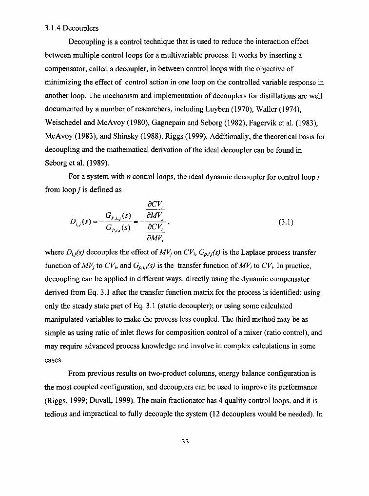
3.1.4 Decouplers
Decoupling is a control technique that is used to reduce the interaction effect
between multiple control loops for a multivariable process. It works by inserting a
compensator, called a decoupler, in between control loops with the objective of
minimizing the effect of control action in one loop on the controlled variable response in
another loop. The mechanism and implementation of decouplers for distillations are well
documented by a number of researchers, including Luyben (1970), Waller (1974),
Weischedel and McAvoy (1980), Gagnepain and Seborg (1982), Fagervik et al. (1983),
McAvoy (1983), and Shinsky (1988), Riggs (1999). Additionally, the theoretical basis for
decoupling and the mathematical derivation of the ideal decoupler can be found in
Seborg etal. (1989).
For a system with n control loops, the ideal dynamic decoupler for control loop /
from loopy is defined as
dCV,
Gp^Xs) dMV.
dMV,
where Di/s) decouples the effect of MVj on CVt, Gpj/s) is the Laplace process transfer
fimction of MVj to CVt, and Gpxi(s) is the transfer function of MVj to CVj. In practice,
decoupling can be applied in different ways: directly using the dynamic compensator
derived from Eq. 3.1 after the transfer function matrix for the process is identified; using
only the steady state part of Eq. 3.1 (static decoupler); or using some calculated
manipulated variables to make the process less coupled. The third method may be as
simple as using ratio of inlet flows for composition control of a mixer (ratio control), and
may require advanced process knowledge and involve in complex calculations in some
cases.
From previous results on two-product colunms, energy balance configuration is
the most coupled configuration, and decouplers can be used to improve its performance
(Riggs, 1999; Duvall, 1999). The main fractionator has 4 quality control loops, and it is
tedious and impractical to fully decouple the system (12 decouplers would be needed). In
33

fact, as shown by the open loop responses in the previous section, the process is not a
fully coupled system, and some of the quality loops have only one-way coupling. For
example, the LCO reflux does not have significant impact on the top and HCN product
qualities, while the top pumparound duty has significant impact on the LCO end point.
Table 3.3 shows the steady state gain array of the base case configuration, in which a
blank indicates that an MV only has negligible effect on the corresponding CV. Based on
this information, the number of decouplers needed to fully decouple the system can be
reduced to 7. However, it is still tedious to design and tune 7 decouplers. In addition, as
the system becomes more complex, maintenance becomes more difficult, and reliability
of the system is reduced. Hurowitz (1999) has shown in his study on superfractionators
that complex two-way decouplers may actually result in inferior performance. Therefore,
only simple decoupling techniques are preferred in the industry, in which one or two
simple decouplers are used to improve performance of the most important product quality
control loops.
For main fractionators, a popular decoupling technique used in industry (Hsie,
1989) is static decoupler, which uses total product flow above a side product draw tray to
control quality of that side product. Since the LCO product quality is controlled by LCO
reflux in this study, the simple decoupling technique is only applicable to HCN product
quality control, i.e., the TBP end point of HCN is controlled by manipulating the total
flow of the overhead liquid distillate and the HCN product. This is implemented in this
study as a comparison to PI and DMCPlus''"' controls. The only configuration change for
this implementation is that the total flow of the overhead liquid distillate (manipulated by
the top level) and the HCN product is used as the manipulated variable by the HCN
endpoint controller, as show in Figure 3.5.
Table 3.3 Steady state gains
Qpi (MMBTU) Fpi (Ibmol/sec) L22 (Ibmol/sec) 0 P 6 (MMBIU)
EPi (F) -6.21
-5.29
EP3 (F) -1.72 0.017
-1.62
EP4(F) -1.08 0.0224 -0.094 -3.42
API2 (F)
0.0077 0.201
34

- ^ Gas to Compressor
GE3^ r^ r<S>""
- j ^ i — •
Decant Water
To Absorber
Naphtha |"T"[» ^
stripper ^^tfTS. ''
Heavy Naphtha
Figure 3.5 Simple decoupler implementation
3.1.5 Tuning Controllers
Both the diagonal PI confroUers and PI with the simple decoupler were tuned with
a similar approach adopted by previous studies on two-product colunms (Anderson,
1999; Duvall, 1999; Hurowitz, 1998). In this approach, ATV tests are performed to each
quality confrol loop, and the ultimate gain Kuj and period /*„,, are identified from the test
results for each loop (AsfrOm and Hagglund, 1984). Then, the Tyreus and Luyben
(1992) controller gains and reset times are determined as follows.
K^,=K„,/3.22 (3.2)
r5=2.2P„, (3.3)
Finally, a detiuung factor FD is used to adjust the gains and reset times on line.
K„ I = K^i I Fn c,/ (3.4)
^c, = S^z, (3.5)
Note that the same detuning factor is applied to all four quality confrol loops, after
the initial settings are calculated from ATV test results for all four quality confrol loops
35

and the bottom temperature overtide control. The detuning factor for the temperature
controller is determined first using a 5 °F decrease in the bottom temperature setpoint
with all quality control loops in manual mode. Then, with the temperature overrider in
function, following setpoint change sequences are used to determine the best detuning
factor for quality control loops.
1. At a time of 0.2 hours, the top product endpoint setpoint is decreased by 5 °F
from the initial steady state value.
2. At a time of 10 hours, the top product endpoint setpoint is decreased by 5 "F
again.
3. At a time of 20 hours, the HCN product endpoint setpoint is decreased by 5 °F.
4. At a time of 30 hours, the HCN product endpoint setpoint is increased by 5 °F,
back to its initial value.
5. At a time of 40 hours, the top product end point setpoint is increased by 5 °F
6. At a time of 50 hours, the top product endpoint setpoint is increased by 5 °F,
back to its initial value.
7. At a time of 60 hours, the simulation ends.
The detuning factor with the minimum lAE is selected. The same tuning method
is applied to quality control loops for both the PI controllers without decoupler and the PI
controllers with a simple decoupler. Tables 3.4 and 3.5 present the tuning results for the
simple PI controllers and PI controllers with simple decoupler, respectively. In the case
of PI with decoupling, during the ATV tests for the top, bottom and LCO loops, the total
flow of top and HCN products is held constant. In the case of PI without decoupling, the
HCN product flow is held constant. As indicated by Tables 3.4 and 3.5, although the
decoupling is only applied to the HCN endpoint control loop, the gains and reset times
for other loops are also changed.
After the quality confrol loops are tuned, two feed composition step changes, a
2% lighter feed and a 2% heavier feed, are used to test the control performance. The 2%
heavier feed is simulated by switching 2% mole fraction from the lighter 50% mole
fraction materials in the initial feed to the heavier 50% mole fraction materials, and
distributing the change among components proportionally to its initial composhion. The
36

results are presented in Figs. 3.6-7, and will be discussed later with the DMCPIUS^M
control results.
Table 3.4 Tuning parameters for the PI controllers without decoupler applied to the main fractionator
Controller
Top
Bottom
HCN
LCO
Temperature
TL Gain
1.033 (MMBTU/hr/F)
83.796 (MMBTU/hr/APl)
71.1 (Ibmol/hr/F)
11.84(lbmol/hr/F)
2.096 (MMBTU/hr/F)
TL Reset Time
0.400
0.2222
0.7111
0.32222
0.13333
FD
4
4
4
4
1
Table 3.5 Tuning parameters for the PI controllers with a simple decoupler applied to the main fractionator
Controller
Top
Bottom
HCN
LCO
Temperature
TL Gain
0.541 (MMBTU/hr/F)
59.854 (MMBTU/hr/API)
53.92191003 (Ibmol/hr/F)
9.87 (Ibmol/hr/F)
2.096 (MMBTU/hr/F)
TL Reset Time (hr)
0.51
0.067
0.9111
0.29
0.13333
FD
4
4
4
4
1
3.2 DMCPlus™ Control
The main fractionator dynamic simulator was interfaced with the DMCPlus^"^
software provided by AspenTech®. Due to the overhead of the communication between
37

the simulator and the DMCPlus^"^ controller, the closed-loop simulation is slowed down
to 3 times faster than real time.
DMCPlus''"' control is a multivariable control algorithm that uses linear step
response models to predict fiiture responses of controlled variables, and then arrange
ftiture control moves based on the prediction trying to minimize the controlled variable
deviations from their targeted values. Process constraints in manipulated and controlled
variables can be explicitly handled in the DMCPIUSTM controller. Handling process
deadtime, coupling and feed forward for measured disturbance are built-in functionalities
of DMCPlus™ controls.
3.2.1 Controller Implementation
For the application of DMCPIUS^M to the main fractionator, level controls are not
included in the DMCPIUS^M controller. PI level controls as discussed in the previous
section are used for various case studies. Feed disturbances are considered unmeasured
and not included as part of the DMCPIUS^M controller. Thus, the DMCPIUS^M controls the
four product qualities and the bottom temperature, and has four manipulated variables:
the top and bottom pumparound duties, the HCN product flow, the LCO reflux flow.
Step tests are conducted by using 2% step changes in Qpi, Qpe, Fpi and 20% step
changes in L22. Big relative change used for L22 because its absolute value is very small
and small changes do not have significant response. A 4x5 step response model is
identified from the step test results using the DMCPlus''"' Model software. The model has
a time to steady state of three hours, and 150 model coefficients are used. The control
interval is 72 seconds. The controller is tuned by using the same setpoint change
sequences as used for the decentralized controllers. The final tuning parameters with the
best setpoint tracking performance are listed in Table 3.6 for CVs and Table 3.7 for MVs.
The controller is then tested with the same disturbances used to test the PI controllers,
and the results are presented in the following section.
38

Table 3.6 Tuning parameters for CVs in the DMCPlus''"' controller for the main fractionator
CVName
ECE for High Limh
ECE for Low Limh
ECE for Middle
SS ECE for High Limh
SS ECE for High Limh
Low Limit Rank
High Limit Rank
Transition Zone Width at High Limit
Transition Zone Width at
High Limit
Low Limit
High Limit
EPi
0.005 F
0.005 F
0.005 F
0.005 F
0.005 F
2
2
0
0
331 F
331 F
API2
0.05
0.05
0.05
0.05
0.05
2
2
0
0
7.31
7.31
EP3
0.005 F
0.005 F
0.005 F
0.005 F
0.005 F
2
2
0
0
674.3 F
674.3 F
EP4
0.005F
0.005F
0.005F
0.005F
0.005F
2
2
0
0
400 F
400 F
T40
0.01 F
I F
I F
0.01 F
I F
6
1
lOF
lOF
690 F
670 F
Table 3.7 Tuning parameters for the MVs in the DMCPlus''"' controller for the main fractionator
MVName QPi > i L22 QP6
Move Suppression 0.04 0.04 0.04
Max Move 0.4MMBTU/hr 10 Ibmol/hr 2 Ibmol/hr
Max LP Step lOMMBTU/hr 200 Ibmol/hr 100 Ibmol/hr
0.04
0.4 MMBTU/hr
lOMMBTU/hr
39

3.3 Results and Analysis
Table 3.8 shows the Integral Absolute Error (lAE) statistics of the three
controllers for the setpoint change sequence. The simple decoupler improves control of
the HCN and LCO endpoints, but sacrifices the top product endpoint and the bottoms
API control. The DMCPlus'' ' controller loosens the bottoms API control, and performs
significantly better than both the PI controllers with and without a decoupler on endpoint
control of other three products.
Tables 3.9-10 show the lAE results for the three controllers subjected to the
heavier and lighter feed changes. Overall, the DMCPlus™ controller outperforms both
PI controllers with and without a decoupler. The DMCPlus^"^ controller has the capability
of scaling the relative importance between multiple controlled variables using Equal
Concem Errors (ECE). In this case, 0.05 API deviation has the same concern to the
controller as 0.005 °F deviation in endpoints as listed in Table 3.4. The DMCPlus™
controller makes compromises between API and endpoint controls according to this
information. The results show that the DMCPlus^"^ controller pays less attention to the
API control, and better endpoint controls are obtained compared to the PI controllers. On
the other hand, each PI controller tries to do its own job to its best, but there is no
coordination between multiple loops. The simple decoupler only provides partial
coordination between loops. That is why the PI controllers did a good job on the API
control, but performed poorly on controlling the endpoints, which is the more important
objective in this process.
Figures 3.6 and 3.7 show the dynamic responses of the controlled variables to the
heavier and lighter feeds, respectively. These results are consistent with the lAE results
discussed above. Both the PI controllers with and without a decoupler have very sluggish
response for top product endpoint in order to reduce upset to the bottom control loops.
The PI controller without decoupling has a steady state offset in the LCO endpoint
response. This is caused by unnecessary tight confrol on the bottoms API. The PI
controller with the simple decoupler and the DMCPlus''"' controller remove this offset by
applying less tight control on the bottoms API.
40

Table 3.8 lAEs for setpoint changes
EPi(F-h) EP3(F-h) EP4(F-h) APl2(API-h)
PI 31.1
PI with decoupler 35.5
DMC 4.9
45.4
24.0
20.1
49.7
47.7
3.6
0.48
0.72
3.80
Table 3.9 I AEs for a heavier feed change
EPi(F-h) EP3(F-h) EP4(F-h) APl2(APl-h)
PI 12.6
PI with decoupler 9.3
DMC 3.0
2.5
1.9
1.2
2.7
1.2
1.8
0.03
0.13
0.14
Table 3.101 AEs for a lighter feed change
Epi(F-h) EP3(F-h) EP4(F-h) APl2(API-h)
PI 6.8
PI with decoupler 5.8
DMC 1.4
1.6
1.0
0.69
1.8
1.7
1.0
0.056
0.043
0.050
41

QL UJ
340
336 •
332 •
328
i!i \ x^^^, /
/ DMCPlus
'*^*^,„^^ ^ PI with Decoupler ^ ^ ' " " ^ ^ * ^ ^ - * ^ ^ ^ ^ P'
0 1 2 3 4
Time (hr)
a. Top product 90% TBP endpoint response to a heavier feed
CO Q. LU
405
403
401 •
399
DMCPlus
0 1 2 3 4
Time (hr)
b. HCN product 90% TBP endpoint response to a heavier feed
Figure 3.6 Responses to a heavier feed
42

1-a. ui
684
680
676
672
DMCPlus
PI with Decoupler
PI
0 1 2 3 4 5
Time (hr)
c. LCO product 90% TBP endpoint response to a heavier feed
7.40
7.35 •
7.25
7.20
DMCPlus
1 2 3
Time (hr)
d. Slurry product 90% TBP endpoint response to a heavier feed
Figure 3.6 Continued.
43

692
684
DMCPlus
PI with Decoupler
1 2 3
Time (hr)
e. Bottom temperature response to a heavier feed
Figure 3.6 Continued
332
324
DMCPlus
p. PI with Decoupler
2 3 4
Time (hr)
a. Top product 90% TBP endpoint response to a lighter feed
Figure 3.7 Responses to a lighter feed.
44

402
CO 4 0 0 Q. LU
398
I ' \
DMCPlus
PI with Decoupler
I I
2 3
Time (hr)
b. HCN product 90% TBP endpoint response to a lighter feed
Q. LU
676
674
672
670
, DMCPlus
PI with Decoupler
J . J .
1 2 3
Time (hr)
c. LCO product 90% TBP endpoint response to a lighter feed
Figure 3.7 Continued.
45

7.40
DMCPlus
7.25 •
7.20
PI with Decoupler
0 1 2 3 4
Time (hr)
d. Slurry product 90% TBP endpoint response to a lighter feed
692
e. Bottom temperature response to a lighter feed
Figure 3.7 Continued.
46

3.4 Discussion of Results
The main fractionator process is a highly coupled system. The DMCPlus^"^
controller outperforms the decentralized control systems in most cases because it has
built-in decoupling power, and ability to scale importance between multiple control
objectives. Decouplers can improve performance of PI controllers significEmtly.
However, tuning and implementation are not convenient and still performed in an ad hoc
way. A 2x2 system may be the largest system to be feasibly decoupled in the industrial
settings. The more complex the control system is, the more difficult it is to maintain,
hence, more likely, it would be tumed off due to poor performance and difficulties in
understanding.
47

CHAPTER 4
MODELING OF A GAS RECOVERY UNIT
This chapter presents the steady state design and dynamic model development for
the gas recovery unit. Section 4.1 provides an overview of the process and its steady state
design parameters. The model is based on a depropanizer model developed by Duvall
(1999). Modifications and additions made to the depropanizer model are presented in
Section 4.2.
4.1 Process Description
The GRU process studied in this work was originally designed by Boyden and his
colleagues at AspenTech as a linear example in his DMCPlus "* training classes. It was
redesigned with ChemCAD with only minor changes. The steady state flow rates and
product compositions were benchmarked against the original design (Boyden, 1999), and
are presented in Table 4.1. The design parameters for each column are used as input for
the dynamic simulator, and listed in Table 4.2.
Table 4.1 Summary of stream properties for the GRU process
stream No. Stream Name Temp C Pres psia Enth Btu/sec Vapor mole : Total std V
fraction sc
Component mole Methane Ethane Propane N-Butane N-Pentane N-Hexane
fh fractions
1 GRU Feed 32.2222 450.0000 -35126. 0.00000
805193.81
0.049 0.180 0.253 0.406 0.060 0.052
2 DC2 Feed 71.1111 445.0000 -33556. 0.023416 805193.81
0.049 0.180 0.253 0.406 0.060 0.052
48

Table 4.1 Continued.
stream No. Stream Name Temp C Pres psia Enth Btu/sec Vapor mole fraction Total std V sc Component mole Methane Ethane Propane N-Butane N-Pentane N-Hexane
Stream No. Stream Name Temp C Pres psia Enth Btu/sec
fh fract
Vapor mole fraction Total std V sc Component mole Methane Ethane Propane N-Butane N-Pentane N-Hexane
Stream No. Stream Name Temp C Pres psia Enth Btu/sec Vapor mole f Total std V Component mc Methane Ethane Propane N-Butane N-Pentane N-Hexane
:rai sc: lie
fh fract
ction fh fract:
3 DC2 Bot 126.2013 448.0000 -24834. 0.00000
585495.75 ions
0.000 0.006 0.297 0.544 0.082 0.071
5 Fuel Gas 29.4444
439.7000 -6480.7 1.0000
219698.14 ions
0.180 0.643 0.137 0.039 0.001 0.000
7 DC4 Feed 111.8329 233.7000 -19043. 0.00000
407731.84 ions
0.000 0.000 0.012 0.768 0.117 0.102
4 DC3 Feed
86.3940 443.0000 -26405. 0.00000
585495.75
0.000 0.006 0.297 0.544 0.082 0.071
6 Propane Fuel
43.0643 219.7000 -7023.3 0.00000
177763.94
0.000 0.020 0.950 0.030 0.000 0.000
8 Propane 42.2709
219.7000 -6665.9 0.00000
169343.83
0.000 0.020 0.970 0.010 0.000 0.000
49

Table 4.1 Continued.
stream No.
Stream Name Temp C Pres psia Enth Btu/sec Vapor mole ; Total std V
fraction sc
Component mole Methane Ethane Propane N-Butane N-Pentane N-Hexane
fh
9 Butane
58.1278 90.0000 -15513. 0.00000
326386.91 fractions
0.000 0.000 0.015 0.955 0.030 0.000
10 C5 +
121.5511 99.3000 -4502.8 0.00000
81345.17
0.000 0.000 0.000 0.020 0.468 0.512
The process diagram is shown in Figure 4.1. The unit includes a deethanizer, a
depropanizer and a debutanizer. The feed is a mixed hydrocarbon stream with C1-C5+
material, and passes through a feed/bottoms heat exchanger en-route to the deethanizer.
This heat exchanger provides heat to partially vaporize the feed. Hence, a mixed phase
feed enters the deethanizer. Products of the unit include "rich" fuel gas (with 10-20 mol%
of C3+ material), liquid and vapor propane, mixed butanes, and C5+ streams. The
propane vapor is vented to the fiiel gas system, so its value is that of fuel gas, not the
propane.
The deethanizer is actually a stripper, and its feed enters at the top tray of the
column. The overhead vapors that do not condense in the deethanizer condenser are
vented out as the fuel gas. The accumulator pressure is confroUed by adjusting the fuel
gas vent flow. Deethanizer reflux is on flow control. The deethanizer accumulator level
is maintained by an operator manually. Cooling water is used to condense the tower
overhead. However, the condenser is undersized and the cooling water valve is always
wide open during operation. The steam to the reboiler is on flow control. The bottom
level is directly controlled by adjusting the valve on the line to the depropanizer. The
deethanizer is typically not a bottleneck, but it can be flooded if overloaded.
50

Table 4.2 Design parameters for the GRU columns
Total Number of Trays'
Feed Tray Location^
Column Pressure
Murphree Tray Efficiency
Reflux Ratio
Reflux Condition
Feed Condition^
Accumulator Residence Time
Reboiler Residence Time
Tray Hydraulic Time Constant
Above Feed Tray
Tray Hydraulic Time Constant
Below Feed Tray
Composition Analyzer Delay
Composition Sampling Rate
Deethanizer
36
35
439.7 psia
0.75
1.942
Saturated
Partially
vaporized
lOmin
5 min
4 sec
3 sec
5 min
5 min
Depropanizer
40
23
219.7 psia
0.7
3.089
Saturated
Subcooled
liquid
5 min
5 min
4 sec
3 sec
5 min
5 min
Debutanizer
30
17
90.0 psia
0.7
0.623
Saturated
Saturated
liquid
5 min
5 min
4 sec
4 sec
5 min
5 min
Note: 1. Number of trays includes reboiler and condenser 2. Trays are counted from the bottom to top with the reboiler as tray 1. 3. Feed and product flow rates and compositions are listed in Table 4.1
The depropanizer has a partial condenser. The pressure is controlled via a hot
vapor bypass around the overhead condenser. When this system is overloaded, the hot
vapor bypass valve closes off completely and pressure control of the system is lost. At
this point, the propane vent to fuel gas has to be opened to off-load the condenser.
However, under normal operation, since the vapor propane is vented to low value fuel gas
system, the vent valve is fiilly closed. The accumulator level is controlled by adjusting
propane product flow rate. There is a storage limit for the liquid propane on-site, so at
times, the production of liquid propane is restricted. The depropanizer is the throughput
51

bottleneck in the unit, and can be easily overloaded. When it floods, the depropanizer
typically experience jet flooding.
The debutanizer condenser is operated as a flooded condenser. There is no level
measurement of liquid level in the condenser. The overhead pressure is controlled by
adjusting the liquid product (mixed butanes) flow, and is an effective indicator of liquid
level in the condenser. The tower is typically not a bottleneck, but it can be flooded if
overloaded.
All three towers are reboiled by steam from the same utility, and use cooling
water from the same source for condensers. There are purity specifications on the liquid
propane, butane and C5+ streams. Two gas chromatograph analyzers are installed, one on
the liquid propeme stream, the other on the mixed butane stream. To save cost, each
analyzer measures two impurities: C2 and C4 in the propane product, C3 and C5 in the
butane product. The operation of a downstream tower is highly dependent on its upstream
towers, so the system is highly interactive. For example, when a constraint in the
depropanizer is met, one has to adjust control handles located in the deethanizer and the
debutanizer to stabilize the system.
52

> o u 2 00
I o
03 CO u u o
i 00
53

4.2 Model Development
The rigorous tray-to-tray model used for the GRU columns are based on a
depropanizer model developed by Duvall (1999). Pressure dynamics and pressure drop
calculations are added in order to model the pressure controls and the flooding
constraints. Simple heat exchanger models are also included to model the feed/bottoms
heat exchanger and the condensers. Same model assumptions as used in Duvall (1999)
are adopted. Additionally, the hydraulic time constants for trays are assumed to have
values listed in Table 4.2.
At each time step, the heat and mass balances as well as the VLE equilibrium
equations are solved first by assuming a constant pressure profile in column. Then the
pressure change is calculated according to a mass balance in the vapor phase, 2md the
pressure drop through each tray is calculated using a steady state correlation between the
pressure drop and the liquid-vapor traffic on that tray. Dynamic VLE calculations are
described in detail in Duvall's work (1999), hence, will not be repeated here. The pressure
dynamics, the pressure drop calculation and the heat exchanger dynamic model are
described as follows.
4.2.1 Pressure Dynamics
For the high-pressure columns in the GRU process, the relative changes in
pressures are typically small, and have negligible effect on phase equilibrium and
enthalpy calculations (Choe and Luyben, 1987). Hence, the mass and energy balances
and the phase equilibrium model are solved first by assuming constant tray pressures. To
keep track of the pressure change in the accumulator, a vapor mass balance is applied to
the accumulator.
'-f-V.-V-K (4.1)
where Mv= moles of vapor in the accumulator
V= vapor distillate molar flowrate
VT = molar vapor flowrate leaving the top tray in the column entering the
condenser.
54

Z,c= molar flowrate of vapor being condensed to liquid in the condenser.
Then, the specific volume of vapor is calculated from
v = (V,„,-V,)/My (4.2)
where V,oi= the total free volume in the accumulator,
VL= the volume occupied by the liquid in the accumulator, which can be
calculated from the liquid mass balance.
Finally, the pressure can be estimated by solving the SRK equations for the vapor
phase as following.
SRK(P,v,T^,yi,)^0 (4.3)
where P = the system pressure,
TD - temperature in the accumulator,
yo = vapor composition in the accumulator.
The model described above ignores vapor holdups in the trays and the reboiler,
resulting in too fast pressure responses. Hence, the value of V,oi is adjusted during
simulations to obtain reasonable pressure dynamics.
4.2.2 Heat Exchanger Dynamic s
Heat exchangers have fast dynamics compared to distillation columns and other
unit operations in a process. Normally the time constant is measured in seconds but could
be up to a few minutes for large exchangers. Process-to-process exchangers should be
modeled rigorously by partial differential equations since they are distributed systems, in
order to estimate the correct amount of deadtime and time constant in the exit stream
temperatures. However, the resulting models are inconvenient to solve, especially in
large-scale plantwide process simulations. Luyben et al. (1999) found that for the purpose
of plantwide control studies it was not necessary to build such detailed models of heat
exchangers, since these units rarely dominate the process response. They recommended a
simplified approach, in that one can use the effectiveness method to calculate the steady
state exchanger exit temperatures and then delay these temperatures by first-order time
constants to capture the dynamics. This approach is adopted to model the feed/bottoms
heat exchanger and is extended to model the condensers in this study.
55

The effectiveness method is used extensively as rating equations for an existing
heat exchanger design (Gebhart, 1971; Jones and Wilson, 1997) to determine the exit
temperatures under different operating conditions. The effectiveness of an exchanger
shown in Fig. 4.2 is defined as
„_ (^C,)„(r, -T,) _ (mC,),(T, -T,) _ Q imC,)^ST,-T,) (mC,)^,„(T-T,) (mC,)^,„(T-T,)'
where (mCp)u = product of flowrate and specific heat capacity of the hot stream,
(mCp)(. = product of flowrate and specific heat capacity of the cold stream,
(wCp)„i„ = the smaller of (mCp)^^ and (mCp)^,,
Ti = hot stream inlet temperature,
T2 = hot stream exit temperature,
T3 = cold stream inlet temperature,
T4 = cold stream exit temperature,
Q = heat transferred.
Ti
T4
/ ^
. M L "V ' cs V
T3
T2
Figure 4.2 Heat exchanger
For a given values of inlet flows and temperatures, the exit temperatures are
explicitly calculated for a known exchanger effectiveness:
56

€(mCp)^,„(T,- T^
(rhCp)„ T=T^-——;:^"; ' - , (4.5)
^^^^^^s(mCp)^.AT,-T,) ^^^^ (mCp)„
The effectiveness is determined by the exchanger's design parameters through the
following equation:
l-g-c-'')'^"^)
I-re' ^ ~ 1 ..--0-r)N7V) ' (4.7)
where r = ^"^^^^""" , (4.8) (ff^Cp)^^
UA NTU = - — - ^ , (4.9)
UA = product of the overall heat transfer coefficient and the heat transfer area,
(mCp) i„ = the larger of (mCp) „ and (mCp )c .
Both r and NTU arc weak functions of temperature in most cases. Therefore, for
dynamic simulation around some nominal operating condition, the effectiveness can be
assumed constant, and calculated from the initial condition.
The dynamics of the feed/bottoms heat exchanger in the GRU process is modeled
in the following way.
1. Calculate the effectiveness at the initial steady state using Eq. 4.4.
2. At each time step, calculate the steady state exit temperatures using Eqs. 4.5-
6.
3. To get the current exit temperatures, delay the exit temperatures calculated
above by a first-order filter with a time constant of 6 seconds, e.g., for the hot
stream exh temperature, T2(t+At)=T2(t)*(l-At/6)+T^^2*(At/6).
4. The exit enthalpies are calculated based on the temperatures.
4.2.3 Condenser Heat Transfer Dynamics
Usually, the cooling duty of distillation condenser can be manipulated freely by
adjusting the coolant flow rate, when refrigeration is used, or by adjusting a hot vapor
57

bypass around the condenser. In previous distillation control studies, cooling duty is used
as a manipulated variable to control the overhead pressure (Lundstrom and Skogetad,
1995), or the pressure control is assumed perfect and the cooling duty is not calculated
(Duvall, 1999). Heat transfer dynamics of the condenser is not modeled.
In the GRU process, the deethanizer condenser is undersized. The cooling water
valve is always wide open, and there is no hot vapor bypass. Hence, the cooling duty can
not be adjusted freely. Consequently, cooling water temperature becomes a significant
disturbance to the tower, hence, to the whole unit. It is necessary to model the heat
transfer dynamics to capture the effect of this disturbance.
The effectiveness method described above can be used to calculate the steady
state cooling duty with known overhead temperature and the cooling water temperature:
Q^=€(mCp),AT,-Tc^) (4.10)
where Ty = the overhead vapor temperature,
Tcfv = the cooling water temperature,
(mCp )cw ~ product of the cooling water flowrate and specific heat capacity.
The hot side of condenser involves phase change, hence, has larger heat capacity.
The cooling water heat capacity is used in the above equation.
The steady state cooling duty is delayed by using a first-order time constant to
model the heat fransfer dynamics, similar to the approach used for the feed/bottoms heat
exchanger.
For the flooded debutanizer condenser, the effectiveness is not a constant because
the heat transfer area decreases as more cooling water tubes are covered by the
condensate (i.e., UA is not a constant). To simplify the model, the heat transfer area is
assume to be proportional to available vapor volume in the shell side the condenser:
UA(t) = K,(V,„,-V,^(t)), (4.11)
where Vugft) = volume occupied by liquid in the shell side of the condenser at time t,
Vtot = total volume of the condenser shell side,
Ki = constant.
58

At each time step, the liquid volume can be back calculated from the Uquid
material balance, and Eq. 4.11 is substituted into Eq. 4,9 to calculate the effectiveness.
Then the cooling duty can be calculated using Eq. 4.10.
For the condenser on the depropanizer overhead shown in Fig.4.3, the effect of
the bypass on heat fransfer has to be taken into account. When the bypass is fully closed,
the situation is the same as the deethanizer condenser, and the condenser reaches its
maximum cooling capacity. As the bypass flow increases, the cooling duty decreases
because less vapor is condensed. Hence, to avoid complexity, the cooling duty is assumed
proportional to the fraction of vapor flow that enters the condenser, that is,
Qc=i^-LMr^Cp)cATv-Tc^) (4.12)
where^ = fraction of the bypass flow.
When the valve is fiilly open,^ =1.0. When the valve is fully closed,yft =0.0. In
between, the value of^ is assumed the same of the valve position in percentage of
opening.
Figure 4.3 Depropanizer overhead section
It should be noted that the condenser heat fransfer models presented here are just
approximations. However, they are reasonable enough to represent following confrol-
relevant process behaviors and consfraints.
59

1. As the temperature difference between the overhead vapor and cooling water
decreases, the cooling duty decrease.
2. As the bypass opens, the cooling duty decrease.
3. When the bypass fully closes, the condenser reaches its cooling constraint
4. As the condenser is fully flooded, the condenser reaches its cooling constraint.
5. Increasing the cooling water flow increases the cooling duty.
4.2.4 Pressure Drop
In distillation control, the pressure drop across the column is used as an indicator
of flooding, and is controlled as a constraint. The high limit for the pressure drop control
is set to a value below the actual flooding onset pressure drop. The pressure drop across
each tray can be calculated from steady state design equations.
For valve trays, when valves are fully opened, the dry pressure drop caused by
vapor flow is
AP,,.^ = / : , A.,„v.', (4.13)
where Ki = constant, determined by the design parameters,
Pvin = density of the vapor that flows into the tray,
Vh = vapor velocity through the holes in the tray.
When valves are partially open, the dry pressure drop is calculated from
AA,.^ = Y^^-'^'y + ^3A/„, > (4.14)
where K2, K3 = constant, determined by the design parameters,
Pm = density of the metal in valves,
tm = thickness of valves.
The actual dry pressure drop is the larger of the two calculated above, that is
AP,^=maK(AP,,^,AP,,^). (4.15)
In this study, all three columns are operated near their maximum capacities.
Therefore, the dry pressure drop is calculated via Eq.4.13.
The pressure drop caused by liquid passing through the tray is calculated by
60

AP.. = 0.4/?, GPM
2/3
+ A,. (4.16)
where pi = density of liquid on the tray,
GPM= liquid load on the tray (gallon per minute),
Lw = weir length,
hw = weir height.
Hence, the total pressure drop across the tray is
(4.17)
61

CHAPTER 5
GRU CONTROL
Both the decentralized control and the DMCPlus^"^ control are applied to the
GRU process. Section 5.1 presents implementation details of the decentralized control
system. Three different DMCPlus''"'*^ control implementations are presented and compared
in Section 5.2. The performances of the decentralized control system and the
DMCPlus^'^ controller are compared in Section 5.3. Finally, results are discussed in
Section 5.4.
5.1 Decentralized Control for GRU
There are multiple control objectives that have to be met for the GRU process.
First, the column pressures have to remain stable, and the levels of liquid inventories
have to be regulated within a certain limits for safe operation. Second, impurity
specifications on propane and butane products have to be maintained in face of various
disturbances such as the feed composition, flow, and temperature changes, the cooling
water temperature changes. Third, process constraints, including the flooding limits on all
three columns and the maximum propane product flow, should not be violated. Finally,
the total vent of fuel gases from both the deethanizer and the depropanizer overheads
should be minimized, while the propane and butane production should be maximized.
5.1.1 Configuration Considerations for the Quality Controls
For convenience of discussion and the control project management, each control
loop for the GRU process is assigned to a control point name. All the control points are
listed in Table 5.1. For each point, there are three variables/values can be used: controller
setpoint, controller output, controlled variable measurement. These variables are
identified with tag names. A tag name starts with the name of the point to which it
belongs, followed by a dot, followed by "SP" for the setpoint, or "PV" for the CV
measurement, or "VP" for the contoller output if the controller directly manipulating a
62

flow control valve. If the controller is cascaded to another controller, then its output is the
setpoint to its slave controller, and no tag is needed for the output of the master
controller. For example, Fl.SP, Fl.PV, Fl.VP mean the setpoint of flow controller Fl,
flow measurement, and valve position of the control valve manipulated in the Fl loop,
respectively. Similarly, T3.SP, T3.PV mean the setpoint measurement of the temperature
control loop T3, respectively. But, as shown in Figure 3.1, T3 is cascaded to F5.
Therefore, the tag name for T3 output is F5.SP, and no separate tag name for T3 output is
needed.
All three columns are high relative volatility, low reflux ratio columns. For the
deethanizer, only the mole fraction of C2 in the stream leaving at the bottom has to be
controlled. It is measured by an analyzer on the propane stream (Al .PV). The content of
the heavy components (C3+) in the overhead fuel gas does not require tight control. The
debutanizer has the similar situation, in which only the impurity of the top product
(A4.PV) is controlled. Therefore, these two columns only require single-ended
composition control, and the [L,V] configuration is the natural choice (Duvall, 1999;
Hurowitz, 1998; Anderson, 1998). The depropanizer in the GRU process is similar to the
depropanizer studied by Duvall (1999), and it requires tight composition control on both
ends, i.e., C3 in the butane product (A3.PV) and C4 in the propane product (A2.PV). It
has been shown in Duvall's work that the [L,V] configuration is still the best
configuration except for high purity cases (impurity less than 1%). In the base case of this
study, the mole fraction of C3 in the butane product is 1.5% and the mole fraction of C4
in the propane product is 3%. Therefore, [L,V] configuration is also chosen for the
depropanizer. Table 5.2 details the CVs and MVs and their pairings with the tag name
notation described above.
63

Table 5.1 Control point names used for GRU process control.
Point Name Description A1 A2 A3 A4 F1 F2 F3 F4 F5 F6 F7 F8 F9 F10 F11 F12 F13 F14 F15 T1 T2 T3 T4 T5 T6 T9 T51 L01 L02 LOS L04 105 P01 P02 P03 P51 PD01 PD02 PD03
Mole Fraction of C2 in Propane Mole Fraction of C4 in Propane Mole Fraction of C3 in Butane Mole Fraction of C5 in Butane GRU Feed Flow/Throughput Deethanizer Reflux Flow Deethanizer Reboiler Steam Depropanizer Fuel Gas Vent Depropanizer Reflux Propane Product Debutanizer Reflux Butane Product C5+ Product Depropanizer Reboiler Steam Debutanizer Reboiler Steam Deethanizer Bottoms Flow Depropanizer Bottoms Flow Deethanizer Fuel Gas Vent Depropanizer Condenser Hot Vapor Bypass Flow Deethanizer Overhead Temperature Deethanizer Bottom Temperature Depropanizer Top Inferential Tray Temperature Depropanizer Bottom Inferential Tray Temperature Debutanizer Top Inferential Tray Temperature Debutanizer Bottom Temperature GRU Feed Temperature Cooling Water Temperature Deethanizer Bottom Level Deethanizer Accumulator Level Depropanizer Bottom Level Depropanizer Accumulator Level Debutanizer Bottom Level Deethanizer Overhead Pressure Depropanzer Overhead Pressure Debutanizer Overhead Pressure Steam Head Pressure Pressure Drop Across the Deethanizer Column Pressure Drop Across the Depropanizer Column Pressure Drop Across the Debutanizer Column
64

Table 5.2 Configuration for GRU decentralized control.
CV MV
Ll.PV F12.SP
L2.PV F2.SP
L3.PV F13.SP
L4.PV F6.SP
L5.PV F9.SP
Pl.PV F14.SP
P2.PV F15.VP
P3.PV F8.SP
Al.PV T2.SP
T2.PV F3.SP
A2.PV T3.SP
T3.PV F5.SP
A3.PV T4.SP
T4.PV FIO.SP
A4.PV T5.SP
T5.PV F7.SP
5.1.2 Constraint Handling
There are four major constraints in this unit: maximum propane production,
deethanizer flooding limit, and depropanizer flooding limit and debutanizer flooding
limit. Pressure drop across each column is measured, and excessive pressure drop is used
as an indicator for flooding. That is, a high limit is specified on each column's pressure
drop, and the control system has to maintain all three pressure drops below those limits.
PID override controls Eire implemented to satisfy these requirements. Table 5.3
summarizes implementation of the four override controls for the constraints described
above.
65

For the flooding constraint of the deethanizer, there could be two options:
reducing the reboiler steam flow or reducing the feed. Both options can reduce vapor-
liquid traffic in the column. However, reducing the reboiler steam flow will sacrifice the
composition Al control, and increase the load of depropanizer, which is the bottlenecking
unit in the plant and operated at its 95% capacity. Consequently, flooding in the
depropanizer would most likely occur if we choose to reduce the deethanizer reboiler
steam in case of flooding in the deethanizer. Therefore, reducing the feed, i.e., the GRU
throughput, is the only choice to handle the deethanizer flooding limit in this case.
In case of flooding in the depropanizer, we also have two options to reduce the
column load: reducing the depropanizer reboiler steam; and increasing the deethanizer
reboiler steam to reduce feed to the depropanizer. Reducing the depropanzier reboiler
steam sacrifices A3 control, resulting in off-spec butane product, while increasing the
deethanizer reboiler steam only result in overpurified propane. Therefore, increasing the
deethanizer reboiler steam is the more reasonable approach to handle this constraint.
When the debutanizer is about to be flooded, reducing the debutanizer reboiler
steam is the natural approach to reduce the vapor traffic in the column. Increasing the
depropanizer reboiler steam in this case may cause flooding in the depropanizer.
In case that the propane product flow rate (F6.PV) reaches its high limit, the top
inferential tray temperature setpoint (T3.SP) is reduced to overpurify the propane, hence
make less propane production.
Constraint
Table 5.3 Implementation of the four override controls
Overrider MV Overrided Controller Selector Type
PDOl.PV high limh Fl.SP
PD02.PV high limh F3.SP
PD03.PV high limh Fll.SP
F6.PV high limh T3.SP
Throughput
Al
T6
A2
Low select
High select
Low select
Low select
66

5.1.3 Inferential Control
Inferential controls in this study are implemented via a cascade control approach,
in which each composition controller adjusts a tray temperature controller setpoint. As
shown in Table 5.2, all four composition controls (A1-A4) are cascaded to tray
temperature controls. The best tray temperature is located for each composition by using
the approach described in Riggs (1998). Table 5.4 shows the trays used to infer
compositions A1-A4.
Table 5.4 Tray temperatures used to infer compositions.
Composition Tray
A1 Deethanizer Tray # 16 from the bottom
A2 Depropanizer Tray #32 from the bottom
A3 Depropanizer Tray #12 from the bottom
A4 Debutanizer Tray #23 from the bottom
5.1.4 Tuning PID Controllers
Level and pressure controllers are tuned by a straightforward trial-error approach
using level and pressure setpoint changes. Table 5.5 shows the timing parameters for all
the pressure and level controllers implemented for the GRU process. All level controllers
are tuned sluggish in this study, i.e., small gains and large reset times are used for level
controllers. The advantage of using sluggish level controllers can be illustrated by an
analysis on the situation of the deethanizer bottom level control (LI controller). The
bottoms stream of the deethanizer is heat integrated with the GRU feed stream. If we tune
LI controller tightly, any change in the level will result in rapid adjustment of the
bottoms flow. This rapid change will not only be a disturbance to the depropanizer, but
also affect the heat duty of the bottoms-feed heat exchanger, thus affect the temperature
of the feed to the deethanizer. As a result, tight level control for the deethanizer bottom
may cause severe oscillation to the deethanizer, and amplify disturbance to the
depropanizer. In industrial practice, sluggish level controllers are popularly used to
67

prevent the disturbance recycle due to heat integration, and reduce possibility of the
disturbance amplification to down stream units (Boyden, 1999).
Table 5.5 Tuning parameters for pressure and level controllers
Integral Time (sec)
4:0x10^
5.0x10^
2.0x10^
2.0x10^
2.0x10^
2.0x10^
2.0x10^
5.0x10^"
After the pressure and level control loops are closed, ATV tests are conducted to
obtain ultimate gains and periods for the temperature controls. Then temperature setpoint
changes are used to tune each temperature controller. Table 5.6 lists the final tuning
parameters used for all temperature controllers.
Table 5.6 Tuning parameters for temperature controllers
Contt-oll
LI
L2
L3
L4
L5
PI
P2
P3
er Gain
2.0x10"-'(sec"')
1.0x10" (sec"')
1.0x10" (sec"')
1.0x10" (sec"')
2.0x10"^ (sec"')
2.0x10' (Ibmol/sec/psia)
2.0x10"^ (Ibmol/sec/psia)
1.0x10" (Ibmol/sec/psia)
Controller
T2
T3
T4
T5
T6
Gain
1.0x10^ (BTU/sec/"C)
1.0x10" (lbmol/sec/°C)
2.0x10^ (BTU/sec/°C)
1.0x10" (Ibmol/sec/'C)
1.0x10^ (BTU/sec/°C)
Integral Time (sec)
2.0x10'
5.0x10^
5.0x10^
5.0x10^
5.0x10^
68

With temperature, pressure and level controls in function, ATV tests are
performed for each composition control loops. Ultimate gains and periods are identified
from the ATV test results. Tyms and Luyben (1992) controller gains and reset times are
determined as described in Chapter 3. Then the online detuning factor is searched for by
using 25% relative changes in composition setpoints. Table 5.7 shows the tuning results
for the composition controls. The same detuning factor is applied to A2 and A3
controllers because they control separation in the same (depropanizer) colunrn.
Table 5.7 Tuning parameters for composition controllers
Controller
Al
A2
A3
A4
Gain (°C/%mol)
521.0
480.0
600.0
450.0
Integral Time (sec)
6600.0
1500.0
2000.0
1500.0
Detuning Factor
0.7
1.5
1.5
1.0
Finally, the override controllers are also tuned by trial-error using setpoint
changes. During on-line tuning of an override control, the controller overrided by this
overtider is tumed off For example, when the depropanizer flooding override control is
tuned, the Al control is tumed off Table 5.8 shows the final tuning parameters used for
the override controllers.
Table 5.8 Tuning parameters for override controllers
Constraint
PDOl
PD02
PD03
F6
Gain
0.5 (Ibmol/sec/psi)
100.0 (BTU/sec/psi)
20.0 (BTU/sec/psi)
100.0 (°C-sec/lbmol)
Integral Time (sec)
500.0
500.0
300.0
200.0
69

5.2 DMCPlus™ Control of GRU
5.2.1 Control Strategy Design
DMCPlusT"^ and other multivariable control technologies provide more flexibility
to implement various control strategies conveniently. However, choosing the best/right
control strategy or configuration for a specific problem is still a challenging problem.
Control experts in the field largely rely on their experience and process knowledge to
guide through the strategy design process. Following is a partial list of major questions to
be answered in a DMCPlus " project on a large-scale control problem like the GRU
process (Boyden, 1999).
1. What are the control objectives? The primary driving force must be economic.
It is essential to identify all of the constraints that limit the profitability of the
process.
2. How many controllers should be built? How is the scope of each controller
defined? The controller should be big enough to cover all the significant
constraints and interactions on accomplishing objectives, yet small enough to
be easily understood by human operators. If an extraordinary big controller is
necessary, it is broken down into sub-controllers according to operating
"units".
3. What CVs, MVs and measured disturbances should be included in each
controller? Make sure all possible measured disturbances are included
directly, even if they are in another unit or DCS system. Use setpoints of
regulatory controllers for MVs and disturbances whenever possible. Avoid
including partially independent variables. All constraints should be included.
Transforms should be considered for non-linearities.
4. What regulatory control loops should we break, and include the CV and MV
directly in the DMCPlus^** controller? In most cases, fast regulatory control
loops working at high frequency remain closed, and their setpoints are used as
MVs. Loops with unsatisfactory performance may be taken out, and their
controls relegated to the model predictive controller. In certain cases.
70

including inventory controls into MPC may be beneficial for quality control
(Huang, 1999).
For the GRU process in this study, handling the constraints in the depropanizer
requires adjustments on operation of the deethanizer, and any change in an upper stream
unit affects the down stream units. Therefore, all three columns interact with each other,
and a controller should include all the three columns for maximum flexibility and
coverage of all interactions and constraints in the plant. In most DMCPlus''"' applications,
levels are left out for PI controls. However, the manipulated variable used for the
deethanizer bottom level, the bottoms flow, affects the downstream units £is a disturbemce
and affects the deethanizer via the heat integration with the feed stream. Hence, the
choice regarding the deethanizer bottom level control loop (LI) is not so obvious.
Therefore, three DMCPlus''"'** implementations with different approach to handle the LI
loop are applied to the GRU process:
DMC-1: Leave LI closed, and the DMCPlus'' ' has no control on this level.
DMC-2: Leave LI closed, and the DMCPlus moves the setpoint to LI controller.
DMC-3: Break LI loop, and the DMCPlus^"^ directly control the level by moving
the bottoms flow rate.
Other independent (MVs and FFs) and dependent variables for all three
implementations are listed in Table 5.9. The constraints such as flooding limits and
propane production limit are included explicitly in DMCPlus''"' controls. In addition, the
depropanizer condenser bypass flow is used to control the overhead pressure. As pressure
becomes exceedingly high, the bypass valve will be fiilly closed. In that case, the
DMCPlus' ** controllers need to adjust other variables to maintain the pressure control.
Therefore, the bypass valve position (F15.VP) is included as a controlled variable, and a
low limit (10%) is specified.
71

Table 5.9 Independent and dependent variables included in all three DMCPlus^"^ controllers
Independent Variables Dependent Variables
T2.SP (MV)
T3.SP (MV)
T4.SP (MV)
T5.SP (MV)
T6.SP (MV)
Fl.SP (MV/Feed Forward)
F4.SP (MV)
T9.PV (Feed Forward)
T51.PV (Feed Forward)
Ll.SP (DMC-2 only)
F12.SP (DMC-3 only)
Al.PV
A2.PV
A3.PV
A4.PV
T6.PV
PDOl.PV
PD02.PV
PD03.PV
F6.PV
F15.VP
Fl.PV
Ll.PV (DMC-2 and DMC-3 only)
5.2.2 Tuning DMCPlus™ Controllers
After step tests are conducted, step response models for the three DMCPlus^"^
controllers are identified. All three controllers use a control interval of one minute. The
time to steady state for step response models in all three controllers is 210 minutes.
Twenty-five percent changes in A2 and A3 setpoints are used to tune all three
DMCPlus^"^ controllers. Due to the large dimension of the tuning parameters, no
minimum lAE search is performed. In order to make the comparison between three
implementations as fair as possible, the DMC-1 controller is tuned first with reasonable
responses, and the tuning parameters are used as the base case. Then, the DMC-2
controller is tuned by using the same tuning parameters as used in DMC-1 for all MVs
and CVs other than the LI .SP and LI .PV. Only tuning parameters for LI .SP (move
suppression) and Ll.PV (ECEs) are adjusted to get better setpoint tracking results.
72

The DMC-3 controller includes the deethanizer bottom level as a ramp variable.
This introduces two more tuning parameters: the ramp rate and the rotation factor,
compared to DMC-2. The ramp rate is the fraction of error between current value and the
user specified level setpoint to be eliminated by the controller in one time to steady state.
The rotation factor is defined as fraction of the model prediction error that is attributed to
the material imbalance in the process, i.e., ramp disturbance. Starting with the same move
suppression factors and ECEs as used in DMC-2, the rotation factor is first determined by
monitoring the model prediction error for Ll.PV. Then, the ramp rate is adjusted to get
the best composition setpoint tracking responses. Finally, move suppression factors are
adjusted one by one to obtain better setpoint tracking responses. The setpoint change
sequences used for tuning are as follows.
1. At time of 1 hour, A3 setpoint decreases by 25% of its initial steady state
value.
2. At time of 7 hours, A3 setpoint increases by 20% back to its initial steady
state value.
3. At time of 13 hours, A2 setpoint decreases by 25% of its initial steady state
value.
4. At time of 19 hours, A2 setpoint increases by 25% back to its initial steady
state value.
5. At time of 25 hours, the simulation stops.
73
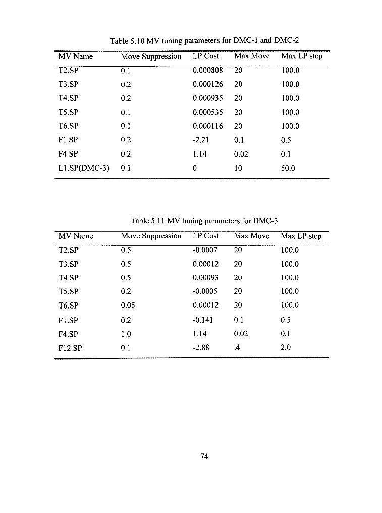
Table 5.10 MV tuning parameters for DMC-1 and DMC-2
MVName Move Suppression LP Cost Max Move Max LP step
T2.SP
T3.SP
T4.SP
T5.SP
T6.SP
Fl.SP
F4.SP
Ll.SP(DMC-3)
0.1
0.2
0.2
0.1
0.1
0.2
0.2
0.1
0.000808
0.000126
0.000935
0.000535
0.000116
-2.21
1.14
0
20
20
20
20
20
0.1
0.02
10
100.0
100.0
100.0
100.0
100.0
0.5
0.1
50.0
Table 5.11 MV tuning parameters for DMC-3
MVName Move Suppression LP Cost Max Move Max LP step
T2.SP
T3.SP
T4.SP
T5.SP
T6.SP
Fl.SP
F4.SP
F12.SP
0.5
0.5
0.5
0.2
0.05
0.2
1.0
0.1
-0.0007
0.00012
0.00093
-0.0005
0.00012
-0.141
1.14
-2.88
20
20
20
20
20
0.1
0.02
.4
100.0
100.0
100.0
100.0
100.0
0.5
0.1
2.0
74

Table 5.12 CV tuning parameters for all three DMCPlus™ controllers
CV name
ECEs for high limh
ECE for low limh
ECE in the middle
ECE for SS high limh
ECE for SS low limh
Rank for high limh
Rank for low limit
CV name
ECEs for high limit
ECE for low limit
ECE in the middle
ECE for SS high limh
ECE for SS low limh
Rank for high limit
Rank for low limit
Rotation factor (DMC-3)
Ramp rate (DMC-3)
CV name
ECEs for high limit
ECE for low limh
ECE in the middle
ECE for SS high limit
ECE for SS low limh
Rank for high limit
Rank for low limit
Al
0.001
0.002
0.002
0.001
0.002
3
4
LI (DMC-2 and
DMC-3 only)
0.01
0.01
200
0.01
0.01
1
1
0.1
0.1
F15.VP
0.05
0.05
0.05
0.05
0.05
1
1
A2
0.001
0.002
0.002
0.001
0.002
3
4
PDOl
0.01
1
1
0.01
1
1
6
A3
0.001
0.002
0.002
0.001
0.002
3
4
PD02
0.01
1
1
0.01
1
1
6
A4
0.001
0.002
0.002
0.001
0.002
3
4
PD03
0.01
1
1
0.01
1
1
6
T6
5
5
5
5
5
5
6
F6
0.01
1
1
0.01
1
2
6
Fl
0.1
0.1
0.1
0.1
0.1
6
5
75

5.2.3 Results
After the DMCPlus^"^ controllers are tuned, they are tested with two unmeasured
feed composition step changes as disturbances: a 10% heavier feed and a 10% lighter
feed. The 10% heavier feed is simulated by switching 10% mole fraction of C3 and
lighter materials to C4 and heavier materials, while the 10% lighter feed is simulated by
switch 10% mole fraction of heavy materials to light materials. The changes are
distributed among the components in the feed proportionally according to their original
composition. Figures 5.1-5.2 present composition responses of all three implementations
to these two disturbances. Table 5.4 shows the lAE comparison between the three
implementations. As shown by these results, DMC-2 has almost the same performance of
control on Al as DMC-1 for the heavier feed, while DMC-3 has poor Al response to the
lighter feed. In other cases, both DMC-2 and DMC-3 outperform DMC-1. These resuhs
agree with the results that has been obtained in a previous study on single column control
(Huang, 1999). That is, when a manipulated variable used for level control has significant
effects on compositions, including that level control into MPC controller will improve the
composition control. The reason is as follows. A PI controller that controls a level cares
about nothing but the level. Therefore, if the level control loop is coupled with a
composition control loop, the PI level controller actually generates disturbance to the
composition loops. When the level control is included in MPC, the MPC can make
compromise between the level control and the composition control, hence achieve better
composition control by swinging the level.
Comparing DMC-2 with DMC-3, DMC-2 has advantages in tuning and step test.
For step test, it is difficult to maintain levels within a certain limits without the PI level
controllers in function, especially when the process is very slow. For tuning, includmg
each level into MPC as a ramp variable introduces two more tuning parameters compared
to DMC-2: the rotation factor and the ramp rate. In addition, transition from DMC-1 to
DMC-2 is very easy: one only needs to do additional step tests for the level setpoint, and
tune the move suppression factor for the level setpoint.
76

f l u e
j y o
2%
1%
DMC-2^^^^ fA.
i * ^L
DMC-1
^ /DMC-3
100 200
Time (min)
300
a. C2 in Propane response
tn U
U
3.5%
3.0%
2.5%
2.0%
DMC-2
DMC-3 DMC-1
100 200
Time (min)
300
b. C4 in propane response
Figure 5.1 DMCPIUSTM confrol composition responses to a heavier feed.
77

2.5%
2.0%
1.5%
1.0%
100 200
Time (min)
300
c. C3 in Butane response
4%
u .S 3% •n O
3%
Ij
DMC-2 -
^ 1 • 1
i f l
• " ^ ^
^DMC-1
" f ^ ^ - P - C ^
DMC-3
100 200
Time (min)
300
d. C5 in Butane response
Figure 5.1 Continued.
78

m O G
U
2.5%
2.0%
1.5%
1.0%
DMC-3
-1
DMC-2
V \J •
^ "" J" — ^
DMC-1
•
0 100 200
Time (min)
300
a. C2 in propane response
3.5%
O .S 3.0%
2.5%
0
DMC-1 DMC-3
DMC-2
100 200
Time (min)
300
b. C4 in propane response
Figure 5.2 DMCPlus ** confrol composition responses to a lighter feed.
79

2.0%
0 100 200
Time (min)
300
c. C3 in butane response
u
u
3.5%
3.0%
2.5%
DMC-3 DMC-1
. DMC-2
2.0%
0 100 200
Time (min)
300
d. C5 in Butane response
Figure 5.2 Continued.
80

Table 5.13. lAE reduction compared to DMCPIUS^M without level included
Heavy Feed
DMC-2
DMC-3
Lighter Feed
DMC-2
DMC-3
C2 in C3
- 1 %
13%
7%
-23%
C4 in C3
24%
19%
26%
25%
C3 in C4
27%
19%
30%
24%
C5 in C4
8%
27%
18%
31%
5.3 Comparing the Decentralized Control and the DMCPlus™ confrol
In this section, the results of the DMC-2 controller are compared with that of the
decentralized MIMO control presented in Section 5.1. Figures 5.3 and 5.4 compare
responses of the decentralized and DMCPlus^"^ controls to the heavier feed change.
Figure 5.3 shows that the DMCPlus'' ' controller has better composition controls, even
though the difference is not so significant. However, Figure 5.4a shows that the
DMCPlus''"' controller pushes the depropanizer closer to its flooding limh than the
decentralized control does. Consequently, more propane and butane are produced, and
less fuel gas is vented as shown in Figs. 5.4b-d. This is because the DMCPlus^"^ has a
linear program that determines the final steady state target according to the economic
information (LP costs), and the controller can achieve that target by adjusting multiple
handles simultaneously.
81
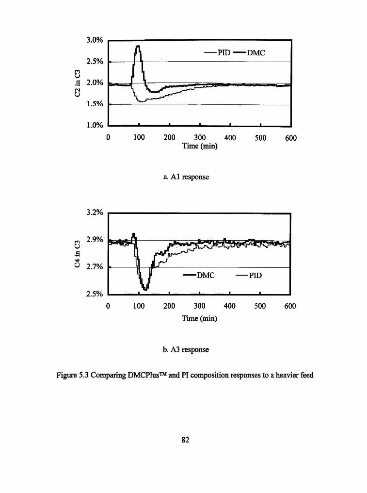
inC
3
o
3.0%
2.5%
2.0%
1.5% »
1.0%
laaEM
A • ^
•
.J/"""'^ z>^ -13=354
•
— P I D -—DMC
•
0 100 200 300 400 Time (min)
500 600
a. Al response
3.2%
2.9% a m O (3
S 2.7%
2.5%
0 100 200 300 400 500 600
Time (min)
b. A3 response
Figure 5.3 Comparing DMCPlus^" and PI composition responses to a heavier feed
82

2.5%
1.0%
0 100 200 300 400 500 600
Time (min)
c. A3 response
3.5%
0 100 200 300 400 500 600
Time (min)
d. A4 response
Figure 5.3 Continued.
83
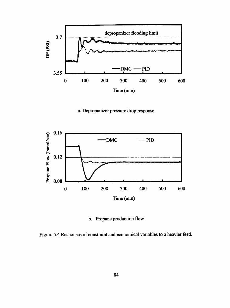
3.7
O
3.55
depropanizer flooding limit
ii»>i uii'''«iiij»i««i< i ' iy i" i i i i i r i r i»i»Vii i rrr iiiif-i i—t- — • ' " " " "
•DMC •FID •
100 200 300 400
Time (min)
500 600
a. Depropanizer pressure drop response
u u
1 O
I
0.16
0.12
0.08 0 100 200 300 400 500 600
Time (min)
b. Propane production flow
Figure 5.4 Responses of consfraint and economical variables to a heavier feed.
84

0.35
0.20
0 100 200 300 400
Time (min) 500 600
c. Butane production flow response
u
o 1 0.16
o
'a "-' 0 1
DMC PID
x ~ ^ _, . . Ir-^
I . . . •
100 200 300 400
Time (min)
500 600
d. Deethanizer overhead fuel gas vent
Figure 5.4 Continued.
85

0.03
1 0.02
^ 0.01
2 0.00
/ \ DMC -
k \^ .
— PID
0 100 200 300 400
Time (min)
500 600
e. Depropanizer overhead fuel gas vent
1.8E+04
1.2E+04 100 200 300 400
Time (min)
500 600
f. Total reboiler heat duty response
Figure 5.4 Continued.
86

Figures 5.5 and 5.6 compare the responses of the decentralized and the
DMCPlusT"^ controls to the lighter feed. In this case, more C3 and lighter materials enter
into the process. As a result, the propane production reaches it maximum limits. The
DMCPlus^"^ controller shows significant advantage in handling this constraint. As shown
in Figure 5.5b, due to the action of the override control, the decentralized system has to
sacrifice the control on A2, which results in a steady state offset. On the other hand, the
DMCPlus^"^ controller finds another way to operate the process to maintain the
constraint, yet not sacrifice the composition control. To meet the maximum propane
production limit, more light materials have to be vented out as fuel gas. As shown in
Figures 5.6a-b, the DMCPlus''"** controller vents more gas out of the deethanizer
overhead, but less gas out of the depropemizer overhead, compared to the decentralized
control system. By doing this, 6% energy is saved as shown in Figure 5.6d, while the
propane production constraint is met as shown in Figure 5.6c. This is due to the fact that
the DMCPlus^"^ controller uses the empirical MIMO process model to make decisions
online, while the PI override control has to pair each constraint with an MV in the offline
design phase. This flexibility of DMCPlus''"' control results in better constraint handling
for MIMO process than the decentralized control.
87

2.4%
^ 2.0%
u c ^ 1.6%
1.2%
i i i i i m
V \r jtr"*""""""
r - ^
DMC -— PID
1
0 100 200 300 400 500 600
Time (min)
a. Al response.
3.4%
0 100 200 300 400 500 600
Time (min)
c. A2 response.
Figure 5.5 Comparing DMCPlus™ and PI composition responses to a lighter feed.
88

1.6%
U 1.2% k
0 100 200 300 400 500 600
Time (min)
c. A3 response.
3.4%
0 100 200 300 400 500 600
Time (min)
d. A4 response.
Figure 5.5 Continued.
89

0.30
0.15
0 100 200 300 400 500 600
Time (min)
a. Fuel gas vented out from the deethanizer overhead
0.02
0 100 200 300 400 500 600
Time (min)
b. The depropanizer fuel gas vent
Figure 5.6 Responses of consfraint and economical variables to a lighter feed
90
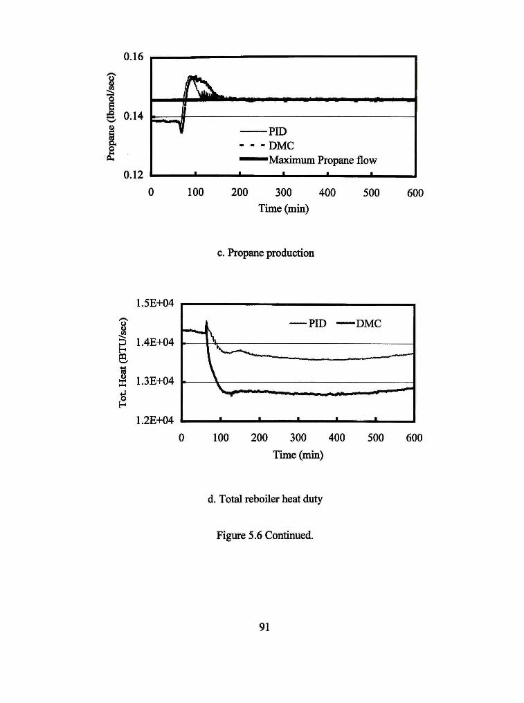
0.16
0.12
u u O)
s
0 100 200 300 400 500 600
Time (min)
c. Propane production
1.5E+04
1.4E+04
X 1.3E+04
E2
1.2E+04
0 100 200 300 400 500 600 Time (min)
d. Total reboiler heat duty
Figure 5.6 Continued.
91

5.4 Discussion of Results
DMCplus^"^ handles constraints better than PID because of hs flexibility.
In certain cases, including level controls into DMCplus''"' can improve
composition control performance. There are two ways of including levels into
DMCplus^"^: direct level control or cascade level control. The DMCplus^"^ cascade level
control has advantages of easy tuning and step test. Studies on single colunms also show
similar results: when an MV for a level control has effect on compositions, including the
level into DMCPlus"*"" (direct or cascade) improves control performance
From a single column control point of view, if [L,V] configuration is used, the
level controllers have no effect on composition control. However, when heat integration
comes into play, level controller timing can have significant effect on the composition
controls. Normally, sluggish level control is preferred from a plantwide control
perspective.
92

CHAPTER 6
CONCLUSIONS AND RECOMMENDATIONS
6.1 Conclusions
In this work, traditional decentralized controls with multiple SISO loops were
compared with model predictive control via rigorous model based simulations on two
complex distillation processes: an FCCU main fractionator and a gas recovery unit. The
DMCPlus^"^ software package is used to implement the MPC controllers, and is
interfaced with the dynamic simulators. It was shown that MPC technology has
significant advantages over the decentralized technology in terms of constraint handling,
decoupling and flexibility, especially for large-scale and complex control problems as
encountered in this study. Table 6.1 details the comparison between MPC and
decentralized control. It should be noted that implementing an MPC controller requires a
great deal of engineering effort, hence it is more suitable for large volume processes
where benefit can be easily justified.
The dynamic simulator for the FCCU main fractionator is based on a rigorous
tray-to-tray model. The model uses the SRK equation to calculate vapor liquid
equilibrium and enthalpies. The dynamic stagewise adiabatic flash (DSAF) algorithm
developed by Chung and Riggs (1995) was extended to solve the dynamic model of the
main fractionator. The algorithm was shown computationally efficient and stable.
Two decentralized control systems, one with a simple decoupler, one without
decoupler, and a DMCPlus^"^ controller were applied to the main fractionator simulator.
The performances of the three controls were compared. The closed-loop simulation
results show that the DMCPlus'' ' controller has significant advantages for handling
multivariable control problem. The capabilities of decoupling, scaling relative importance
of multiple control objectives that are built in the DMCPlus^"^ controller resulted in
significant performance improvement over the decentralized control strategies.
93

Table 6.1
Decoupling
and Feed
Forward
Constraint
Handling
Flexibility
Comparison between decentralized and MPC control strategies
Decentralized Control
•
•
•
•
•
•
•
Each decoupler handles one
interaction.
Ad hoc tuning and
implementation
Inconvenient and unreliable for
large scale problem
One override controller has to
be implemented for each
constraint
Each constraint is paired with
an MV at design time
Relative priorities between
constraints are hardwired in the
control stmcture, i.e., higher
level overrides lower level
When priorities of control
objectives change, the control
stmcture has to be redesigned,
then tuned.
MPC
•
•
•
•
•
•
•
The controller handles all
interactions simultaneously.
Implementation is performed in
a systematic way, automated by
software.
Scalable to any size.
Simply include the constraint as
a controlled variable
No explicit pairing needs to be
specified
Priority for each consfraints are
expressed in tuning parameters
such as ECEs, Ranks, which can
be changed conveniently
Only tuning parameters are
dependent on priorities of
control objectives. No need for
stmctural redesign.
A rigorous model based dynamic simulator was developed for a gas recovery unit,
which consists of three distillation columns operated in series: a deethanizer, a
depropanizer and a debutanizer. The simulator was used to compare the traditional and
model predictive control technologies in terms of handling large dimensional coupling
problem and interactive constraints. The results show that DMCplus'' ' handles
constraints better than PID control because of its flexibility in making decisions on line,
even though PI override can also be used to handle constraints.
94

Three MPC implementations with different strategies for level controls were
applied to the GRU simulator, and their performances were compared. In certain cases,
including level controls into MPC can improve control performance. There are two ways
of including levels into MPC: direct level control, in which the MPC directly control the
level as a ramp by manipulating a flow rate, or cascade level control in which the MPC
moves the level setpoints. The MPC cascade level control has advantages of easy tuning
and step test. Studies on single columns also show similar results: when an MV for a
level control has effect on compositions, including the level into MPC (direct or cascade)
improves performance
From a single column control point of view, if the [L, V] configuration is used,
the level controllers have no effect on composition controls. However, in cases of process
to process heat integration, the level control loop may have significant effect on the
composition controls. Normally, sluggish level control tuning is prefertcd so that
disturbance recycling via heat recycle can be prevented.
6.2 Recommendations
Most of the literature on distillation control is limited to single column control.
This study is an attempt to examine on special issues involved in control of complex
distillation processes. Whether or not the results presented in here can be extended to
more varieties of processes needs to be verified by further studies and industrial practice.
Following recommendations are made for future research in this area.
1. The important draw tray temperatures and product specifications are
benchmarked against published steady state data. However, the dynamic behavior
is not benchmarked due to lack of data. If possible, the main fractionator
simulator should be benchmarked against industtial data.
2. Similarly, benchmark the GRU simulator with industrial data, if any.
3. The inside-out algorithm for the main fractionators is not suitable for simulation
of rapid and big step changes in setpoints and disturbances, because the inner
models have to be updated more often. For the same reason, a relatively good
95

initial condition is needed for this algorithm. A new algorithm is needed for wider
simulation ranges.
4. Measurement noises are implemented on the GRU simulator. However, the effect
of noise on performances of both decentralized control and MPC was not in the
scope of this study. An examination on this issue may be interesting.
5. Heat integration is common in today's industrial processes. More heavily heat
integrated process needs to be studied. For example, the GRU process and the
main fractionator usually interact with each other via heat integration. With these
two simulators in place, an extension may be possible to include the heat
integration schemes between the two processes, and simulate them together.
However, this requires more computation power.
6. MPC relies on properly implemented and tuned regulatory loops as its bottom
layer. In this study, tuning parameters for the regulatory loops (e.g., temperature
controllers) are remained the same when MPC replaces high level decentralized
controls (e.g., composition controllers). However, the tuning that is the best for
the decentralized control may not be the best for MPC applications. A ftirther
study to examine effects of regulatory tuning on performance of MPC is
necessary.
96

REFERENCES
Anderson, J.J., Vacuum Distillation Control, Ph.D. dissertation, Texas Tech University, Lubbock, Texas, 1998.
American Petroleum Institute, Technical Data Book -Petroleum Refining, American Petroleum Institute, Tulsa, Oklahoma, 1981
Apsen Technology Inc., DMCPlus"^^ Multivariable Control Software, Aspen Technology, Inc., Houston, Texas, 1999.
Ayral, T.E., Control improves fractionator performance. Hydrocarbon Processing, 4/1995, pp.87-88.
Barletta, A.F., Revamping cmde units. Hydrocarbon Processing, pp.51-58, Feb. 1998.
Boston, J.F. and Sullivan, S.L., A New Class of Solution Methods for Multicomponent, Multistage Separation Processes, Canadian Journal of Chem. Engr., No 52, 1974, pp.52-63.
Boyden, S., Personal Conunimications, Aspen Technologies, Inc., Houston, Texas, 1997, 1998,1999,2000.
BuUerdiek, E.A. and Hobbs, J. W. Advanced controls pay out in 6 weeks at Texas refinery. Oil and Gas Journal, 6/19/1995, pp.46-52.
Cutler, C.R. and Ramaker, B.L., Dynamic Matrix ControhA Computer Control Algorithm. Presented at the 86th National Meeting of AIChE, Houston, TX, 1979.
Cecchetti, R.; Niedzwiecki, J.L. and Holland, D., Pipestill products verify these computer estimates. Hydrocarbon Processing,42(9), 159(Sept., 1963).
Choe, Y.-S. and Luyben, W.L., Rigorous dynamic models of distillation colunms, Ind. Eng Chem. Res., Vol.26, pp.2158-2161(1987).
Chung, C.-B.; Riggs, J.B., Dynamic simulation and nonlinear-model-based product quality control of a cmde tower, AIChE Jounal, Vol.41, No. 1, pp. 122-134 (1995).
Clinkscales, T.A.; Rice,V. L.; Stanley,!. P., Dynamic, nonlinear, physical model based control and optimization system, AIChE Spring Meeting at Altanta, GA, Session 83, April 17-21, 1994.
97

Duvall, M.P., On Control of High Relative Volatility Distillation Columns, Ph.D. dissertation, Texas Tech University, Lubbock, Texas, 1999.
Ebbesen,L. E., Main fractionator cmde switch control. Computers and Chemical Engineering Suppl. 1997, pp.S165-S 171.
Edmister, ^.C, Applied Hydrocarbon Thermodynamics, Gulf Publishing Co., Houston, Texas, 1984.
Eriksson, P.-O.; Tomlins, A. and Dash, S.K., FCCU advanced control system achieves 2-month payout. Oil and Gas Journal, 3/23/1992,pp62-78.
Fagervik, K., C ; Waller, K.V. and Hammarstrom, L. G., Two-Way or One-Way Decoupling in Distillation? Chem. Eng. Commun, 1983, 21, 235.
Fatora, F.C.; Willet,T.R.; Boyden,S.A.; Haas, D.H. and Icsezen,S., A case study: the DMCPlus controller on the LCR FCC and gas plant, Aspenworld, 1997.
Fleming,B.; Slolely, A.W. and Golden, S.W., Heat integrating fluid catalytic cracking unit fractionation systems, 1994 AIChE Fall meeting, Distillation Column Integration Symposium, ^ov. 11, 1993.
Franks, R.G.E., Modeling, and Simulation in Chemical Engineering, John Wiley & Sons, New York, 1972.
Gagnepain, J.P. and Seborg, D.E., Analysis of Process Interactions with Applications to Multiloop Control System Design. Ind. Eng. Chem. Process Des. Dev., 1982, 21, 5.
Golden, S.W., Case studies reveal common design, equipment errors in revamps, Oil and Gas Journal, 4/7/1997, pp.58-61.
Golden, S.W., Simple engineering change fix product recovery problems, Oil and Gas Journal, 4/14/1997, pp.58-61.
Golden, S.W., Improved control strategies correct main fractionator operating problems. Oil and Gas Journal, 8/21/1995, pp.58-61.
Golden, S.W., Multi-product distillation draw control: revamping for improved operation, AIChE Spring National Meeting, Fractionation in the 90's:Revamps and Retrofitting, Feb . 22-29, 1996.
Golden, S.W.; Martin, G.R. and Slolely, A.W., FCC main fractionator revamps. Hydrocarbon Processing, pp.77-81, Mar.1993.
98

Golden, S.W.; Slolely A.W. and Fleming, B., Revamping FCC main fractionator energy systems. Hydrocarbon Processing, pp.43-49, Nov. 1993.
Gross, F.; E. Baumann; A. Geser; D.W.T. Rippin and L. Lang, "Modeling, Simulation and Controllability Analysis of an Industrial Heat-Integrated Distillation Process", Computers Chem. Eng. Vol.22, No. 1-2, pp. 223-237, 1998.
Hartman,E.L.; Hanson, D.W. and Weber, B., FCCU main fractionator rewamp for CARB gasoline production. Hydrocarbon Processing, 2/1998,pp44-49.
Henson, M.A., Nonlinear Model Predictive Control: Current Status and Future Directions, Computers and Chemical Engineering, Vol. 23, 1998, pp. 187-202.
Hess, F.E., Solution of Equations for Fractionating Columns, Ph.D. Diss., Texas A&M University, College Station, 1977.
Holland, CD., Fundamentals of Multicomponent Distillation, McGraw-Hill, New York, 1981
Hsie, W.-H.L., Modeling, Simulation and Control of Crude Towers, Ph.D. Diss., University of Maryland, College Park, 1989.
Huang, H., Guidelines to interface dynamic simulators with DMCPlus"^^ software. Chemical Engineering, Texas Tech University, 1999.
Huang, H., On applying MPC to 4x4 distillation control, AdChem 2000, Pisa, Italy, 2000.
Hurowitz, S.E., Superfi-actionator Process Control, Ph.D. dissertation, Texas Tech University, Lubbock, 1998.
Jones, D.S.J., Elements of Petroleum Processing, John Wiley & Sons, New York, 1995.
Kister, H.Z., Distillation Operation, McGraw-Hill, New York, 1990.
Kister, H.Z., Distillation Design, McGraw-Hill, New York, 1992.
T.D.V.Lin, FCCU advanced control and optimization. Hydrocarbon Processing, 4/1993, ppl07-114.
Lundstrom, P.; Skogestad, S., Opportunities and Difficuhies with 5x5 Distillation Control, J Proc. Cont., Vol. 5, N. 4, pp. 249-261, 1995.
Luyben, W. L., Distillation Decoupling. AIChE J., 16,198,1970.
99

Luyben, W.L., Process Modeling, Simulation, and Control for Chemical Engineers, 2" ed.,, McGraw Hill, New York, 1990.
Luyben, W.L.; B.D. Tyreus and M.L. Luyben, Plantwide Process Control, McGraw Hill, New York, 1999.
Maxwell, J.B., Data Book on Hydrocarbons, Van Nostrand, New York, 1950.
McAvoy, T.J., Interaction Analysis Theory and Application. Instmment Society of America, Research Triangle Park, NC, 1983.
Mizoguchi, A.; Marlin,T.E. and Hrymak,A. N. "Operations optimization and control design for a petroleum distillation process," The Canadian Joumal of Chemical Engineering, Vol. 73, 1995, pp.896-907.
Qin, S.J. and Badgewell, T.A. An Overview of Industrial Model Predictive Control Technology. In Kantor, J.C, Garcia, C.E.and Camahan, B. (Eds). Chemical Process Control V, CACHE, AIChE, Austin, TX, pp. 232-256, 1997.
Rhemann, H.; Schwarz, G.; Badgwell, T.A.; Darby, M.L. and White, D.C., On-line FCCU advanced control and optimization. Hydrocarbon Processing, 6/1998, pp64-71.
Riggs, J.B., Comparison of Advanced Distillation Control Methods, U.S. Department of Energy Application, Solicitation No. DE-SC04-93AL93300, 1993.
Riggs, J.B., Improve Distillation Column Control, Chemical Engineering Progress, Vol. 94, No. 10, 1998, pp. 31-47.
Riggs, J.B., Chemical Process Control, Ferret Publishing, Lubbock, TX, 1999.
Seborg, D.E.; Edgar, T.F. and Mellichamp, D.A., Process Dynamics and Control, John Wiley 8c Sons, Inc., New York, 1989.
Shinsky, F.G., Process Control Systems, 3"" ed., McGraw-Hill, New York, 1988.
Sims,. J. and Daubert,T.E., Prediction of vapor-liquid equilibria of undefined mixtures, ind. Eng. Chem. Process Des. Dev. 19, 386-393 (1980).
Sofer, S.S.; MulhoUand, R.J. and Bare, W.H., From simple regulatory control to computer optimization. Hydrocarbon Processing, l/1998,pp38-42.
Walas, S., Phase Equilibrium in Chemical Engineering, Butterworth Publishers, Boston, 1985.
100

Waller, K.V., Decoupling in Distillation, AIChE J, 1974,20, 592.
Watkins, R.N., Petroleum Refinery Distillations, Gulf Publishing Company, Houston, Texas, 1979.
Weischedel, K. and McAvoy, T.J., Feasibility of Decoupling in Conventionally-Controlled Distillation Columns, Ind. Eng. Chem. Fundam., 1980, 19, 379.
Zhu, Y., Multivariable process identification for MPC: The asymptotic method and its applications. Journal of Process Control, v.8, n.2, pp. 101-115 (1998).
101