Simulating water hammer with corrective smoothedparticle methodHou, Q.; Kruisbrink, A.C.H.; Tijsseling, A.S.; Keramat, A.

Published: 01/01/2012

Document VersionPublisher’s PDF, also known as Version of Record (includes final page, issue and volume numbers)

Please check the document version of this publication:

• A submitted manuscript is the author's version of the article upon submission and before peer-review. There can be important differencesbetween the submitted version and the official published version of record. People interested in the research are advised to contact theauthor for the final version of the publication, or visit the DOI to the publisher's website.• The final author version and the galley proof are versions of the publication after peer review.• The final published version features the final layout of the paper including the volume, issue and page numbers.

Link to publication

General rightsCopyright and moral rights for the publications made accessible in the public portal are retained by the authors and/or other copyright ownersand it is a condition of accessing publications that users recognise and abide by the legal requirements associated with these rights.

• Users may download and print one copy of any publication from the public portal for the purpose of private study or research. • You may not further distribute the material or use it for any profit-making activity or commercial gain • You may freely distribute the URL identifying the publication in the public portal ?

Take down policyIf you believe that this document breaches copyright please contact us providing details, and we will remove access to the work immediatelyand investigate your claim.

Download date: 17. Jul. 2018

EINDHOVEN UNIVERSITY OF TECHNOLOGY Department of Mathematics and Computer Science

CASA-Report 12-14 May 2012

Simulating water hammer with corrective smoothed particle method

by

Q. Hou, A.C.H. Kruisbrink, A.S. Tijsseling, A. Keramat

Centre for Analysis, Scientific computing and Applications

Department of Mathematics and Computer Science

Eindhoven University of Technology

P.O. Box 513

5600 MB Eindhoven, The Netherlands

ISSN: 0926-4507

Simulating water hammer with corrective smoothedparticle method

Q. Hou1, A.C.H. Kruisbrink2, A.S. Tijsseling1, A. Keramat31Eindhoven University of Technology, The Netherlands2The University of Nottingham, United Kingdom3Jundi Shapur University of Technology, Iran

ABSTRACT

The corrective smoothed particle method (CSPM) is used to simulate water ham-mer. The spatial derivatives in the water-hammer equations are approximatedby a corrective kernel estimate. For the temporal derivatives, the Euler-forwardtime integration algorithm is employed. The CSPM results are in good agreementwith solutions obtained by the method of characteristics (MOC). A parametricstudy gives insight in the effects of particle distribution, smoothing length andkernel function. Three typical water-hammer problems are solved. CSPM willnot beat MOC in classical water-hammer, but it has potential for water-hammerproblems with free surfaces as seen in column separation and slug impact.

1 INTRODUCTION

Transient flow in piping systems is generally caused by rapid changes in flowconditions due to sudden valve operation, pump start up or shut down, powerfailure, etc. The phenomenon is generally called pressure surge or water hammer,and it may damage hydraulic machinery, piping and supports. If possible, itshould be anticipated in the design process and prevented in practice. For detailson transient flow, see the widely used textbook by Wylie et al. [1].

For the simulation of transient flows in pipes, several methods are available.Before the digital computer era, graphical techniques were used. The accuracy ofthis method can be low, since friction is not properly taken into account. The so-lution procedure can be very elaborate and is rarely used nowadays. For details onthe graphical method, interested readers are referred to the summary by Lupton[2]. Nowadays, the most commonly used approach is the computerized methodof characteristics (MOC), which has been employed numerically to simulate tran-sient flow in complex pipe systems since the mid 1960s. Later, water-hammermodels were extended with associated phenomena such as gas release, column sep-aration, unsteady friction, pipe wall viscoelasticity and fluid-structure interaction.Details on MOC and its practice can be found in [1] and the recent review papers[3, 4]. Other methods for the numerical solution of the transient flow equationsinclude the explicit [5] and implicit [6, 7, 8, 9] finite-difference method (FDM),the finite-element method (FEM) [10, 11], Godunov method [12, 13], lattice-Boltzmann method (LBM) [14, 15] and an explicit central-difference scheme withtotal variational diminishing (TVD) [16]. A direct finite-difference methodologywas described in [17], but no results were presented.

In the present paper, the corrective smoothed particle method (CSPM) is usedto simulate transient flow in a reservoir-pipe-valve system. In the CSPM particle

method for the water-hammer problem, the spatial derivatives are approximatedusing corrective kernel estimates. For an acceptable accuracy and high compu-tational efficiency, the temporal derivatives are integrated by the Euler-forwardmethod. To prevent numerical oscillations, an artificial dissipative term is addedto the momentum equation. This artificial viscosity term is switched on in re-gions of high velocity gradients and switched off in smooth regions by evaluatingthe gradient of the particle velocity. The main effects of several key factors onthe performance of CSPM are investigated. These factors are the particle distri-bution (evenly and randomly spaced), artificial viscosity, the kernel or smoothingfunction, smoothing length, pre-smoothing and number of particles.

CSPM is for the first time successfully applied to weakly compressible flow.Water hammer is chosen as a test problem of practical importance, since it hasa validated solution, which is used as a reference. CSPM has been selectedbecause it has potential for simulating water-hammer events that involve freesurfaces, cavitation, liquid slugs and fluid-structure interaction [18, 19]. Water-hammer problems including instantaneous and gradual valve closure, line packand column separation are solved herein.

2 MATHEMATICAL MODELLING

2.1 Governing equations

The governing equations for one-dimensional single-phase transient flow in pipescomprise the following continuity and momentum equations in Eulerian form [1]

∂P

∂t+

[V∂P

∂x

]+ρc2

∂V

∂x= 0,

∂V

∂t+

[V∂V

∂x

]+

1

ρ

∂P

∂x+g

dz

dx+

λV |V |2D

= 0, (1)

where P is the pressure, V is the mean flow velocity, ρ is the fluid density, c isthe sonic wave speed, g is the gravitational acceleration, t and x denote the timeand the axial distance along the pipe, z is the pipe elevation, D is the inner pipediameter, and λ is the Darcy-Weisbach friction factor. Note that the convectionterms between square brackets are usually neglected under the assumption thatV << c. The liquid compressibility, pipe elasticity and wall constraint conditionsare included in the model through the expression for wave speed

c :=

√K

ρ

(1 + ϕ

DK

Ee

)−1

, (2)

in which K is the bulk modulus of the fluid, e is the pipe wall thickness, ϕ denotesthe structural constraint condition of the pipe, for which typical values are givenin [1]. For a pipe, which is free at one end and supplied with expansion joints atregular intervals along its length, the coefficient ϕ is unity.

2.2 Modified momentum equation

For the solution of hyperbolic equations, a dissipative term is usually neededto suppress numerical wiggles. Numerical damping can be introduced explicitly[5, 16] or implicitly [6, 7, 8, 9, 12, 13] in regions of high gradients. For thefast transient flow investigated herein, an explicit dissipative term is added tothe momentum equation, which is called artificial viscosity in smoothed particlehydrodynamics (SPH) [20]. After adding the dissipation term in the momentum

equation, and with constant z and material derivatives, from (1) we get

DP

Dt= −ρc2

∂V

∂x,

DV

Dt= −1

ρ

∂P

∂x− λV |V |

2D+

∂(ρΠ)

∂x. (3)

This Lagrangian form of the continuity and momentum equations will be solvedwith CSPM, as described in Section 4.

3 THE METHOD OF CHARACTERISTICS

The method of characteristics (MOC) is established in the numerical simulationof transient flow in pipelines. It is briefly described in this section. The gov-erning equations of transient flow form a pair of quasi-linear hyperbolic partialdifferential equations (PDEs). They can be transformed via the MOC into apair of ordinary differential equations (ODEs) and then solved by numerical in-tegration. Solving (1) by the MOC for constant z leads to the following so-calledcompatibility and characteristic equations

dV

dt± 1

ρc

dP

dt+

λV |V |2D

= 0,dx

dt= [V ]± c. (4)

The solution of these equations is used as the reference solution in Section 5.

4 CORRECTIVE SMOOTHED PARTICLE METHOD

The corrective smoothed particle method (CSPM), proposed by Chen et al.[21, 22], is a generalization of standard SPH [23]. The key idea of CSPM isto expand the kernel estimate, an essential element in SPH, into a Taylor se-ries. Compared with other modifications to SPH, the CSPM algorithm is quitestraightforward [21]. It not only remedies the two drawbacks in SPH, namelyboundary deficiency [21] and tensile instability [22], but also extends the abilityof SPH in solving PDEs containing second-order derivatives. The two essentialcomponents of CSPM, the corrective kernel estimate and the particle approxi-mation, are described in this section. Since transient flow in pipes is modelledherein as a one-dimensional problem, only those formulations that are requiredin the current work are presented. For the basic theory of CSPM in multi-spacedimensions, see e.g. [21, 22].

4.1 Corrective kernel approximation

Expanding a smooth function f(x) in the neighbourhood of point xi into a Taylorseries, multiplying both sides of the expansion by a smoothing function or kernel,and integrating over the one-dimensional domain Ω yields∫

Ω

f(x)Wi(x)dx =f(xi)

∫Ω

Wi(x)dx+ fx(xi)

∫Ω

(x− xi)Wi(x)dx

+1

2fxx(xi)

∫Ω

(x− xi)2Wi(x)dx+ · · · ,

(5)

where fx := df/dx, fxx := d2f/dx2 and Wi(x) := W (x − xi, hi) is the kernelassociated with point xi. The influence of the kernel is limited to a supportproportional to the smoothing length hi. The influence domain of point xi is theregion where W (x− xi, hi) > 0.

Neglecting all the derivative terms in (5) gives the corrective kernel estimateof the function f(x) at point xi,

f(xi) :=

∫Ωf(x)Wi(x)dx∫ΩWi(x)dx

. (6)

The hat symbol denotes an approximation throughout this work. For a symmetrickernel, the second term at the right-hand side (RHS) of (5) vanishes for interiorregions, but does not so for boundary regions because of a truncated support.The corrective kernel estimate of the function expressed in (6) is therefore oforder h2

i accuracy for points xi far away from the boundary, and of order hi forpoints xi near or on the boundary.

If the kernel Wi(x) in (5) is replaced by its derivative Wi,x := dWi(x)/dx andthe second and higher derivative terms are neglected, a corrective kernel estimateof the first-derivative fx(x) is generated as

fx(xi) :=

∫Ω[f(x)− f(xi)]Wi,xdx∫Ω(x− xi)Wi,xdx

. (7)

The CSPM kernel estimate of the first derivative is also second-order accuratefor the interior points and first-order accurate for the points near or on theboundary [21]. The derivative of the kernel must be anti-symmetric to avoid azero denominator in (7).

4.2 Particle approximation

Taking care that the spatial domain is represented by particles, formulas (6)and (7) are integrated per particle volume. This results in a weighted volumesummation over the particles. If the particle volume is replaced by its mass todensity ratio, the so-called particle approximations become

fi :=

∑Nj=1 fjWij mj/ρj∑Nj=1 Wij mj/ρj

=

∑j∈Si

fjWij mj/ρj∑j∈Si

Wij mj/ρj, (8)

fi,x :=

∑Nj=1(fj − fi)Wij,x mj/ρj∑Nj=1(xj − xi)Wij,x mj/ρj

=

∑j∈Si

(fj − fi)Wij,x mj/ρj∑j∈Si

(xj − xi)Wij,x mj/ρj. (9)

in which fi := f(xi), fj := f(xj), Wij := W (xj − xi, h), fi,x := fx(xi) andWij,x := Wi,x(xj), N is the total number of particles in the domain, and mj andρj are the mass and density of particle j, respectively. The kernel associated withparticle i has a compact support that is much smaller than Ω, so that the numberof particles within the summations is actually much smaller than N . Supposethat there are Ni particles in the support of Wi forming the set Si, then we getthe last terms in (8) and (9).

Particle i and the other particles in the support of Wi(x) constitute so-calledinteraction pairs. A particle search needs to be executed to find Si and thus theinteraction pairs ahead of any calculation [20]. Compared with the conventional

kernel estimate of the function f(x) in SPH, i.e. fi :=∑

j∈SifjWij mj/ρj , the

denominator in (8) is the essential correction for the boundary deficiency [21].To avoid (9) becoming singular, at least one other particle should be within theinfluence domain of particle i. The smoothing length hi has to be within a certainrange to meet this requirement. This is in particular important for particles inthe boundary region, because their support is truncated.

4.3 Kernel

A common choice of the kernel is the cubic spline function

W (q, h) :=1

h

2/3− q2 + q3/2, 0 6 q < 1,

(2− q)3/6, 1 6 q < 2,

0, q > 2,

(10)

where q is the distance between two particles scaled by the smoothing length, i.e.q := |x − xi|/h. The cubic spline function and its first derivative are shown inFig. 1. The kernel W is symmetric and its derivative is anti-symmetric.

−2 −1.5 −1 −0.5 0 0.5 1 1.5 2−1

−0.8

−0.6

−0.4

−0.2

0

0.2

0.4

0.6

0.8

1

q

Fu

nct

ion

× h

KernelDerivative of the kernel

Figure 1: Cubic spline function and its derivative.

4.4 Time-integration algorithm

Meshfree particle methods transform PDEs into ODEs in time. To solve theseODEs, a proper time-integration algorithm is needed. A large variety of timeintegration methods is available and any choice will be a compromise betweenaccuracy, computational efficiency and robustness.

For a set of n coupled first-order differential equations of the form

dy/dt = F (y, t), y ∈ Rn, (11)

the evaluation of F (y, t) usually dominates the computational effort. Conse-quently, for efficiency, the number of evaluations within each time step should bekept as small as possible. The term is evaluated only once in the Euler forwardmethod, whereas it is evaluated at least twice in other explicit time-integrationmethods such as modified Euler, Runga-Kutta and leapfrog [24]. Therefore, theconditionally stable Euler forward method is employed in this paper for timemarching. This time-integration algorithm has first-order accuracy.

The solution is advanced from tn to tn+1 according to

Pn+1i = Pn

i +∆t

(DP

Dt

)n

i

, V n+1i = V n

i +∆t

(DV

Dt

)n

i

, (12)

where the superscripts indicate the time level, and the total time derivatives areobtained from (3) as(

DP

Dt

)n

i

= −ρc2(∂V

∂x

)n

i

,

(DV

Dt

)n

i

= −1

ρ

(∂P

∂x

)n

i

−λV ni |V n

i |2D

+

(∂(ρΠ)

∂x

)n

i

.

(13)

The spatial derivatives (∂V/∂x)ni and (∂P/∂x)ni in (13) are approximated usingformula (9) by substituting P and V for f . For the nonlinear friction term, thevelocities at the previous time step are used. The flow chart of the solution pro-cedure is given in the Appendix. The approximation of the artificial dissipationterm (∂(ρΠ)/∂x)ni is less straightforward and is discussed below.

4.5 Artificial viscosity

In this paper, the dissipation term (∂(ρΠ)/∂x)ni is modelled as an artificial vis-cosity [25] for the SPH simulation of shock waves,(

∂(ρΠ)

∂x

)i

=∑j∈Si

mjΠijWij,x, (14)

Πij :=

−αcµij + βµ2

ij

ρ, (Vi − Vj)(xi − xj) < 0,

0, (Vi − Vj)(xi − xj) > 0,

(15)

µij :=hij(Vi − Vj)(xi − xj)

|xi − xj |2 + ηh2ij

, (16)

where α, β and η are constant coefficients, and hij := (hi + hj)/2 is the averageof the smoothing lengths associated to particle i and particle j. The linear (invelocity difference) term in Πij produces a shear and a bulk viscosity, while thequadratic term is equivalent to the von Neumann-Richtmyer viscosity [20]. Theterm ηh2

ij in µij is added to prevent a singularity (for i = j). Herein, α = 1,β = 2 and η = 0.01 are used, which are typically values for shocks [20].

4.6 Particle distribution and boundary particles

In this paper, evenly and irregularly spaced particles are considered. For evenlyspaced particles, four particle distribution patterns often used in SPH are shownin Fig. 2.

• The cell-centered particle distribution (Fig. 2a) is widely used in SPH. How-ever, the Dirichlet boundary condition cannot be imposed exactly, becausethe boundary particles do not lie on the physical boundaries.

• The cell-centered particle distribution with virtual particles (Fig. 2b) al-lows for an exact enforcement of Dirichlet boundary conditions. The totalvolume is overestimated because two virtual particles are added.

• The vertex-centered particle distribution (Fig. 2c) allows for the same treat-ment of interior and boundary particles. The enforcement of Dirichletboundary conditions is also exact. The total volume is slightly overesti-mated.

• The semi-vertex-centered particle distribution (Fig. 2d) also allows for anexact enforcement of Dirichlet boundary conditions. The total volume iscorrect, but the treatment of the particles adjacent to the boundary isslightly different, because the boundary particles have a reduced (50%)volume.

The irregularly spaced interior particles used herein are randomly distributed.The following rule is applied to obtain the particle positions

xi =

0, i = 1,

(i− 1) ∆x+Ri ζ ∆x, i = 2, · · · , N − 1,

L, i = N,

(17)

Figure 2: Evenly spaced particles: (a) cell-centered, (b) cell-centered with virtualboundary particles, (c) vertex-centered, (d) semi-vertex-centered.

where ∆x = L/(N − 1) is the cell size, L is the domain size, Ri ∈ (−0.5, 0.5)is a random number and ζ ∈ [0, 1] is a parameter determining the magnitudeof deviations from the vertex centres. This parameter mimics the physical stateof particles (solid ζ ≈ 0, gas ζ ≈ 1). For the weakly compressible liquid in thesemi-closed system in Fig. 2, ζ = 0.25 is used. The above particle distributionsare examined in Subsection 5.1.

4.7 Boundary and initial conditions

For the waterhammer considered herein, the two boundary conditions are theprescribed velocity at the valve, i.e. V = 0 at x = L, and the constant pressureat the reservoir, i.e. P = Pres at x = 0. For most of the meshfree methods, inparticular those based on weak forms, special attention needs to be paid to theenforcement of Neumann boundary conditions [26]. However, imposing boundaryconditions in CSPM is simple and straightforward. During the solution course,the velocity boundary condition is directly included in the velocity gradient in(13) for the particle at the valve and the particles interacting with it. The sameholds for the enforcement of the pressure boundary condition on the particlesnear the reservoir. The initial condition is given pressure and velocity.

5 SIMULATIONS AND PARAMETRIC CSPM STUDY

CSPM results are presented for a reservoir-pipe-valve configuration (Fig. 3), sub-jected to instantaneous valve closure, and compared to MOC solutions. Theparticles are assumed not to move after valve closure, because water hammer isan acoustic phenomenon where all displacements V · tw << L due to tw = L/cand V << c. The data used in the numerical calculations are for a water-filledsteel pipe [27]: L = 20 m, D = 797 mm, e = 8 mm, E = 210 GPa, K = 2.1 GPa,ρ = 1000 kg/m3, ϕ = 1, Q0 = AV0 = 0.5 m3/s, Pres = 1 MPa and λ = 0.02. Thewave speed calculated from (2) is 1025.7 m/s. The pipe length is divided into 200equal parts and the time increment ∆t = ∆x/c = 9.75× 10−5 s, so the Courantnumber Cr = c∆t/∆x = 1. The simulation time is 0.3 seconds. Since the cellsize is ∆x = 0.1 m and the density is assumed to be constant, the particle massis m = ρA∆x = 49.9 kg.

We first employ the vertex-centered particle distribution (Fig. 2c), which isused as a reference case. The effect of other distributions, artificial viscosity, pre-smoothing, smoothing length, number of particles and kernel function, is studied

Figure 3: Schematic of a reservoir-pipe-valve system.

in the Subsections 5.1 through 5.6. The reference case is a frictionless simulation,i.e. λ = 0, which is a good and extreme test to identify numerical dissipation anddispersion. The smoothing length is hi = ∆x, (i = 1, · · · , 201). Comparisonsbetween the CSPM and MOC solutions are presented in Fig. 4. The CSPM resultsagree well with the MOC solution. The numerical dispersion is eliminated byartificial viscosity. The usual phase errors (unphysical oscillations or wiggles) andamplitude errors (smearing effect) are largely absent here. Consequently, sharpwave fronts are maintained. An overshoot is visible at the first pressure wavefront only, and not in the time history of the upstream velocity. The overshootis about 6 percent of the pressure variation, and it is treated in Subsection 5.3.

0 0.05 0.1 0.15 0.2 0.25 0.3-1

-0.5

0

0.5

1

1.5

2

2.5

3

Time (s)

Pre

ssu

re (

MP

a)

CSPM

Exact

(a)

0 0.05 0.1 0.15 0.2 0.25 0.3-2

-1.5

-1

-0.5

0

0.5

1

1.5

2

Time (s)

Ve

locity (

m/s

)

CSPM

Exact

(b)

Figure 4: Time history of the (a) downstream pressure and (b) upstream velocity.

5.1 Particle distribution

This section demonstrates the effect of particle distributions on the numericalresults, and suggests the proper distribution to be used in CSPM simulations.

5.1.1 Evenly spaced particles

Evenly spaced particle distributions are the most used in CSPM [21, 22, 28]and related methods [20, 26, 29]. Since the cell-centered particle distribution inFig. 2a does not allow exact enforcement of Dirichlet boundary conditions, theother two types shown in Figs. 2b and 2d are examined.

For the particle distribution in Fig. 2b, the virtual boundary particles havethe same mass as the interior particles, because the same volume and constantdensity are assumed. Consequently, we have 202 particles with the same massm, so that the total mass of the system is overestimated (if the virtual particlesare included in the system) because 202m > ρAL = 200m. The smoothinglengths are taken as ∆x, so that each interior particle has two neighbours. Forthe particle distribution in Fig. 2d, the particle masses are m1 = m201 = m/2

and mi = m (i = 2, · · · , 200), so that the total mass is 200 m. The smoothinglengths are h1 = h201 = ∆x/2 and hi = ∆x (i = 2, · · · , 200).

The results obtained for the three particle distributions in Fig. 5 are nearly thesame. The difference is mainly at the first wave front. The details in Fig. 6 showthat the vertex-centered particle distribution generates the smallest overshoot.Other simulations, in which the mass of the virtual particles (Fig. 2b) is m1 =m201 = m/2 and the smoothing length is h1 = h201 = ∆x, were also run.Although all the results were in good agreement with the MOC solution, thevertex-centered particle distribution performed the best.

0 0.05 0.1 0.15 0.2 0.25 0.3-1

-0.5

0

0.5

1

1.5

2

2.5

3

Time (s)

Pre

ssu

re (

MP

a)

Cell-centered with virtual particles

Vertex-centered

Semi-vertex-centered

(a)

0 0.05 0.1 0.15 0.2 0.25 0.3-2

-1.5

-1

-0.5

0

0.5

1

1.5

2

Time (s)

Ve

locity (

m/s

)

Cell-centered with virtual particles

Vertex-centered

Semi-vertex-centered

(b)

Figure 5: Effect of evenly spaced particles on the (a) downstream pressure and (b)upstream velocity.

0 0.5 1 1.5 2 2.5 3 3.5 4

x 10-3

1

1.2

1.4

1.6

1.8

2

2.2

2.4

2.6

2.8

3

Time (s)

Pre

ssu

re (

MP

a)

Cell-centered with virtual particles

Vertex-centered

Semi-vertex-centered

Figure 6: Same results as shown in Fig. 5, but now on a finer scale to show thedetails at the first wave front.

5.1.2 Randomly spaced particles

Randomly spaced particles mimic the meshless situation where the particles gowith the flow. They allow for different ways to determine the particle mass andsmoothing length. Here we examine three of them. First, we consider constantmass and smoothing length. This is averaging – in a sense – and widely used inSPH [23]. Second, the interior particle mass varies according to mi = ρA(xi −xi−1), while at the boundaries m1 = m201 = m. The smoothing length variesaccording to hi = xi − xi−1 (i = 2, · · · , 200) and h1 = h201 = ∆x. Third,

the interior particle mass is computed from mi =12ρA(xi+1 − xi−1), and at the

boundaries m1 = m201 = m. For all particles, the smoothing length is taken asthe maximum distance between two neighbours. We denote these three differentapproaches as RA1 (random approach 1), RA2 and RA3. The results in Fig. 7show that all three cases give reasonable solutions, but not more than that. Theresults of RA3 are the best, and closest to those in Fig. 5.

0 0.05 0.1 0.15 0.2 0.25 0.3-1

-0.5

0

0.5

1

1.5

2

2.5

3

Time (s)

Pre

ssu

re (

MP

a)

RA1

RA2

RA3

(a)

0 0.05 0.1 0.15 0.2 0.25 0.3-2

-1.5

-1

-0.5

0

0.5

1

1.5

2

Time (s)

Ve

locity (

m/s

)

RA1

RA2

RA3

(b)

Figure 7: Effect of random particle distribution on the (a) downstream pressureand (b) upstream velocity.

To examine the effect of the other parameters, the uniform vertex-centeredparticle distribution (Fig. 2c) is used in the following sections.

5.2 Artificial viscosity

Artificial viscosity is modelled herein with the coefficients α = 1 and β = 2 [20].To demonstrate its effect, the problem is also simulated without artificial viscosityby setting the parameters α and β equal to zero. The results of these simulationsare shown in Fig. 8. It clearly demonstrates that artificial viscosity suppressesnumerical dispersion, which pollutes the solution in an unacceptable way.

0 0.05 0.1 0.15 0.2 0.25 0.3-1

-0.5

0

0.5

1

1.5

2

2.5

3

Time (s)

Pre

ssu

re (

MP

a)

Artificial viscosity

No artificial viscosity

(a)

0 0.05 0.1 0.15 0.2 0.25 0.3-2

-1.5

-1

-0.5

0

0.5

1

1.5

2

Time (s)

Ve

locity (

m/s

)

Artificial viscosity

No artificial viscosity

(b)

Figure 8: Effect of artificial viscosity on the (a) downstream pressure and (b) up-stream velocity.

5.3 Pre-smoothing

Although the results of the present method match the MOC solution well, anovershoot at the first wave front is still visible in Fig. 4a. This overshoot canbe removed by pre-smoothing. The pre-smoothing is applied to the velocitydistribution in the first 5 time steps by using the smoothing features of theCSPM function approximation in (8). Then the derivative of the velocity isapproximated from (9) with the smoothed velocity. This idea is from Monaghan[30] for the simulation of Riemann problems. The pre-smoothed CSPM resultsare depicted in Fig. 9. The overshoot is indeed diminished, but now a very small(< 3%) offset is visible (Fig. 9a). This may be attributed to the numerical errorof the CSPM function approximation in (8). The effect of pre-smoothing on thevelocity is too small to be visible in Fig. 9b.

0 0.05 0.1 0.15 0.2 0.25 0.3-1

-0.5

0

0.5

1

1.5

2

2.5

3

Time (s)

Pre

ssu

re (

MP

a)

No presmoothing

With presmoothing

(a)

0 0.05 0.1 0.15 0.2 0.25 0.3-2

-1.5

-1

-0.5

0

0.5

1

1.5

2

Time (s)

Ve

locity (

m/s

)

No presmoothing

With presmoothing

(b)

Figure 9: Effect of pre-smoothing on the (a) downstream pressure and (b) upstreamvelocity.

The velocity histories are in good agreement with the MOC solution. Forthis reason, the focus is only on the pressure histories in the following sections.Furthermore, friction is included (λ = 0.02), and used together with artificialviscosity and pre-smoothing.

5.4 Smoothing length

The two vital parameters in particle methods are the kernel W and the smoothinglength h. For a given kernel, the smoothing length not only determines thenumerical accuracy, but also affects the computational efficiency and numericalstability [23]. To avoid a singularity in (14) (see Subsection 4.2), the smoothinglength must be h > 0.5∆x (for evenly spaced particles).

Two effects of the smoothing length are observed. On one hand, smoothinglengths smaller than 1.0∆x result in dispersion errors as shown Fig. 10a. Thesmaller the smoothing length is, the more severe the numerical oscillations atthe wave fronts become. The dispersion errors are minimized when h is closeto 1.0∆x. On the other hand, smoothing lengths larger than 1.0∆x result innumerical dissipation as shown in Fig. 10b. With increasing smoothing length,the dissipation or smearing effect is increasing, i.e. the wave fronts are less sharpand the amplitudes become smaller. This results in a big discrepancy betweenthe CSPM calculations and the MOC solution.

In conclusion, for the transient flow problem investigated herein, a smoothinglength h between 0.9∆x and 1.5∆x is sufficient to ensure non-singularity and

acceptable accuracy (minimal numerical dispersion and dissipation).

0 0.05 0.1 0.15 0.2 0.25 0.3-1

-0.5

0

0.5

1

1.5

2

2.5

3

Time (s)

Pre

ssu

re (

MP

a)

h=0.55 x

h=0.75 x

h=1.0 x

(a)

0 0.05 0.1 0.15 0.2 0.25 0.3-1

-0.5

0

0.5

1

1.5

2

2.5

3

Time (s)

Pre

ssu

re (

MP

a)

h=1.0 x

h=1.5 x

h=2.0 x

h=2.5 x

(b)

Figure 10: Effect of the smoothing length on the downstream pressure with (a)small values and (b) large values.

5.5 Number of particles

The effect of the number of particles on the CSPM calculations is exhibited inFig. 11a for h = 1.0∆x. The effect mainly reveals as smearing. If only 21 particlesare used, the first peak and period of the pressure history are predicted well, butthe following peaks and amplitudes become less accurate. When more particlesare employed, the smearing effect becomes less significant. Here, 201 particlesare sufficient for acceptable accuracy.

5.6 Kernel function

Thus far the cubic spline kernel in (10) has been used. An alternative kernel isthe modified Gaussian

W (q, h) :=1.04823

h√π

e−q2 − e−4, 0 6 q < 2,

0, q > 2.(18)

The comparison for the two kernels is depicted in Fig. 11b. Although both simu-lations predict the pressure history at the valve well, better results are obtainedwith the cubic spline kernel.

Many other kernels have been employed in meshfree methods [31]. The effectof the kernel not only depends on the specific meshfree method, but also onthe specific problem. It is hard (if not impossible) to determine the optimumkernel, but the cubic spline function has proven its computational efficiency inSPH [20, 31] and it is most widely used in CSPM [21, 22, 28, 32].

6 TYPICAL WATERHAMMER RESULTS

The validity of CSPM for solving waterhammer problems is demonstrated inthree test cases of practical importance.

6.1 Gradual valve closure

The test problem in Section 5 concerns travelling discontinuities generated byinstantaneous valve closure. Such discontinuities pose problems to any numerical

0 0.05 0.1 0.15 0.2 0.25 0.3-1

-0.5

0

0.5

1

1.5

2

2.5

3

Time (s)

Pre

ssu

re (

MP

a)

N=21

N=51

N=101

N=201

(a)

0 0.05 0.1 0.15 0.2 0.25 0.3-1

-0.5

0

0.5

1

1.5

2

2.5

3

Time (s)

Pre

ssu

re (

MP

a)

Cubic spline

Modified Gaussian

(b)

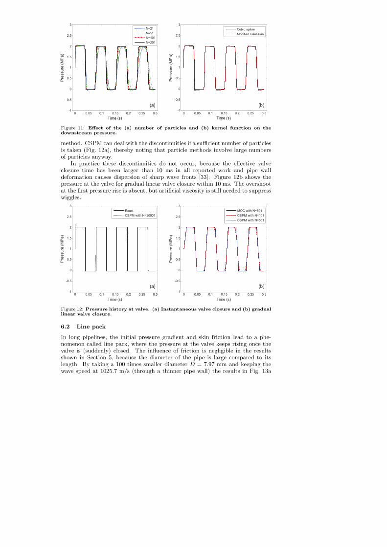
Figure 11: Effect of the (a) number of particles and (b) kernel function on thedownstream pressure.

method. CSPM can deal with the discontinuities if a sufficient number of particlesis taken (Fig. 12a), thereby noting that particle methods involve large numbersof particles anyway.

In practice these discontinuities do not occur, because the effective valveclosure time has been larger than 10 ms in all reported work and pipe walldeformation causes dispersion of sharp wave fronts [33]. Figure 12b shows thepressure at the valve for gradual linear valve closure within 10 ms. The overshootat the first pressure rise is absent, but artificial viscosity is still needed to suppresswiggles.

0 0.05 0.1 0.15 0.2 0.25 0.3-1

-0.5

0

0.5

1

1.5

2

2.5

3

Time (s)

Pre

ssu

re (

MP

a)

Exact

CSPM with N=20001

(a)

0 0.05 0.1 0.15 0.2 0.25 0.3-1

-0.5

0

0.5

1

1.5

2

2.5

3

Time (s)

Pre

ssu

re (

MP

a)

MOC with N=501

CSPM with N=101

CSPM with N=501

(b)

Figure 12: Pressure history at valve. (a) Instantaneous valve closure and (b) graduallinear valve closure.

6.2 Line pack

In long pipelines, the initial pressure gradient and skin friction lead to a phe-nomenon called line pack, where the pressure at the valve keeps rising once thevalve is (suddenly) closed. The influence of friction is negligible in the resultsshown in Section 5, because the diameter of the pipe is large compared to itslength. By taking a 100 times smaller diameter D = 7.97 mm and keeping thewave speed at 1025.7 m/s (through a thinner pipe wall) the results in Fig. 13a

are obtained for the same initial velocity V0 = 1.0 m/s as in Section 5. Line packis clearly visible and predicted well.

6.3 Column separation

Waterhammer not only involves high pressures, but also low pressures. If theabsolute pressure at the valve drops to vapour pressure (0.02 bar for water atroom temperature), the liquid column is separated from the valve by a vapourbubble (or vacuum). This phenomenon is called column separation. It can bemodelled relatively simply by not allowing the pressure to drop below the vapourpressure. A constant (vapour) pressure boundary condition is then prescribedfrom which the downstream velocity of the elastic liquid column, and hence thecavity length, is calculated. The results obtained by CSPM are consistent withthose by MOC, see Fig. 13b. The pressure spike at t = 0.12 s is physical andhas been measured in laboratory test rigs [4]. It is the result of a mismatchof the water-hammer period 2L/c and the time of duration of the first column-separation [1]. The discrepancy between CSPM and MOC is attributed to thewell-known sensitivity of the DVCM model used for column separation.

0 0.05 0.1 0.15 0.2 0.25 0.3-1

-0.5

0

0.5

1

1.5

2

2.5

3

Time (s)

Pre

ssu

re (

MP

a)

MOC with N=501

CSPM with N=501

(a)

0 0.05 0.1 0.15-1

-0.5

0

0.5

1

1.5

2

2.5

3

3.5

4

Time (s)

Ab

so

lute

pre

ssu

re (

MP

a)

MOC with N=501

CSPM with N=501

(b)

Figure 13: Pressure history at valve. (a) Line pack and (b) column separation.

7 CONCLUDING REMARKS

The corrective smoothed particle method (CSPM) is explored for fast transientflow in pipes. To solve the classical water-hammer equations, the time derivativesare approximated by the Euler forward method and the spatial derivatives by thecorrective kernel estimate. The particles were assumed not to move. To suppressoscillations in the transient waves, a dissipative artificial viscosity term is addedto the momentum equation. The CSPM results are in good agreement withconventional MOC solutions. The effect of parameters such as the particle distri-bution, artificial viscosity, smoothing function, smoothing length, pre-smoothingand number of particles has been investigated. The main conclusions are:

• Both uniform and random particle distributions can be used in CSPM. Thevertex-centered particle distribution gives the best results.

• Artificial viscosity is indispensable in the numerical simulations of shocksand contact discontinuities to suppress unacceptable numerical oscillations.

• The pre-smoothing technique can be used to eliminate overshoots at sharppressure wave fronts.

• The smoothing length has a significant effect on the CSPM results. Whenit is taken smaller than 0.9∆x, CSPM suffers from dispersion errors (nu-merical oscillations). When it is taken larger than 1.5∆x, dissipation errors(smearing) appear. In the range between h = 0.9∆x and h = 1.5∆x, where∆x is the distance between particles, good results can be obtained.

• Although many other compactly supported functions can be used as thekernel in CSPM, the cubic spline kernel is the most efficient and accurate.

• Three typical water-hammer problems have been solved successfully withCSPM for the first time.

ACKNOWLEDGEMENT

The first author is grateful to the China Scholarship Council (CSC) for financiallysupporting his PhD studies.

APPENDIX: COMPUTATION STEPS

The flow chart for the simulation of transient pipe flow by CSPM is summa-rized as follows:

• Generate and distribute particles and define associated mass, density andsmoothing lengths

• Loop over all particles:a) Search neighbour particles to establish interaction pairs;b) Calculate discretized kernel Wij and its derivative Wij,x.

• Assign initial pressures and velocities to particles

• Loop over all particles for time marching:1) Apply downstream boundary condition VN = 0;

2) Calculate ∂Vi∂x

by substituting V for f in (9) and obtain DPiDt

from (13);3) Calculate the particle pressure according to (12);4) Apply upstream boundary condition P1 = Pres;

5) Calculate ∂Pi∂x

by substituting P for f in (9);6) Calculate the spatial derivative of the artificial viscosity from (14);7) Calculate the particle acceleration from (13);8) Compute the particle velocity according to (12).

References

(1) Wylie, E. B., Streeter, V. L. and Suo, L. S. (1993). Fluid Transients in Systems. Prentice-Hall: Englewood Cliffs.

(2) Lupton, H. R. (1953). Graphical analysis of pressure surges in pumping systems. Journalof the Institution of Water Engineers, 7: 87–125.

(3) Ghidaoui, M. S., Zhao, M., McInnis, D. A. and Axworthy, D. H. (2005). A review ofwater hammer theory and practice. Appl. Mech. Rev., 58(1): 49–76.

(4) Bergant, A., Simpson, A. R. and Tijsseling, A. S. (2006). Water hammer with columnseparation: A historical review. J. Fluid. Struct., 22: 135–171.

(5) Chaudhry, M. H. and Hussaini, M. Y. (1985). Second-order accurate explicit finite-difference schemes for waterhammer analysis. J. Fluid. Eng., 107: 523–529.

(6) Streeter, V. L. (1972). Unsteady flow calculation by a numerical method. Journal ofBasic Engineering, 94: 457–466.

(7) Tan, J. K., Ng, K. C. and Nathan, G. K. (1987). Application of the centre implicitmethod for investigation of pressure transients in pipelines. Int. J. Numer. Meth. Fluids,7(4): 395–406.

(8) Nathan, G. K., Tan, J. K. and Ng, K. C. (1988). Two-dimensional analysis of pressuretransients in pipelines. Int. J. Numer. Meth. Fluids, 8(3): 339–349.

(9) Arfaie, M. and Anderson, A. (1991). Implicit finite-differences for unsteady pipe flow.Mathematical Engineering for Industry, 3: 133–151.

(10) Jovic, V. (1995). Finite elements and the method of characteristics applied to waterhammer modelling. Engineering Modelling, 8(3-4): 51–58.

(11) Shu, J. J. (2003). A finite element model and electronic analogue of pipeline pressuretransients with frequency-dependent friction. J. Fluid. Eng., 125: 194–199.

(12) Guinot, V. (1998). Boundary condition treatment in 2 × 2 systems of propagation equa-tions. Int. J. Numer. Meth. Eng., 42: 647–666.

(13) Hwang, Y. and Chung, N. (2002). A fast Godunov method for the water-hammer prob-lem. Int. J. Numer. Meth. Fluids, 40(6): 799–819.

(14) Cheng, Y. G., Zhang, S. H. and Chen, J. Z. (1998). Water hammer simulation by thelattice Boltzmann method. Transactions of the Chinese Hydraulic Engineering Society,Journal of Hydraulic Engineering, 6: 25–31 (in Chinese).

(15) Cheng, Y. G. and Zhang, S. H. (2001). Numerical simulation of 2-D hydraulic transientsusing lattice Boltzmann method. Transactions of the Chinese Hydraulic EngineeringSociety, Journal of Hydraulic Engineering, 10: 32–37 (in Chinese).

(16) Wahba, E. M. (2006). Runge–Kutta time-stepping schemes with TVD central differenc-ing for the water hammer equations. Int. J. Numer. Meth. Fluids, 52: 571–590.

(17) Sanchez Bribiesca, J. L. (1981). A finite-difference method to evaluate water hammerphenomena. J. Hydrol., 51: 305–311.

(18) Hou, Q., Zhang, L. X., Tijsseling, A. S. and Kruisbrink, A. C. H. (2012). Rapid fillingof pipelines with the SPH particle method. Procedia Engineering, 31: 38–43.

(19) Hou, Q. (2012). Simulating Unsteady Conduit Flows with Smoothed Particle Hydrody-namics. PhD thesis, Eindhoven University of Technology.

(20) Liu, G. R. and Liu, M. B. (2003). Smoothed Particle Hydrodynamics: A Meshfree Par-ticle Method. World Scientific, Singapore.

(21) Chen, J. K., Beraun, J. E. and Carney, T. C. (1999). A corrective smoothed particlemethod for boundary value problems in heat conduction. Int. J. Numer. Meth. Eng., 46:231–252.

(22) Chen, J. K., Beraun, J. E. and Jih, C. J. (1999). An improvement for tensile instabilityin smoothed particle hydrodynamics. Comput. Mech., 23: 279–287.

(23) Monaghan, J. J. (2005). Smoothed particle hydrodynamics. Rep. Prog. Phys., 68: 1703–1759.

(24) Leveque, R. J. (2007). Finite Difference Methods for Ordinary and Partial DifferentialEquations: Steady-State and Time-Dependent Problems. SIAM, Philadelphia.

(25) Monaghan, J. J. and Gingold, R. A. (1983). Shock simulation by the particle method ofSPH. J. Comp. Physics., 52: 374–381.

(26) Nguyen, V. P., Rabczuk, T., Bordas, S. and Duflot, M. (2008). Meshless methods: Areview and computer implementation aspects. Math. Comput. Simulat., 79: 763–813.

(27) Tijsseling, A. S. (2003). Exact solution of linear hyperbolic four-equation systems inaxial liquid-pipe vibration. J. Fluid. Struct., 18: 179–196.

(28) Chen, J. K., Beraun, J. E. and Jih, C. J. (2001). A corrective smoothed particle methodfor transient elastoplastic dynamics. Comput. Mech., 27: 177–187.

(29) Zhang, G. M. and Batra, R. C. (2004). Modified smoothed particle hydrodynamicsmethod and its application to transient problems. Comput. Mech., 34: 137–146.

(30) Monaghan, J. J. (1997). SPH and Riemann solver. J. Comp. Physics., 136: 298–307.

(31) Fulk, D. A. and Quinn, D. W. (1996). An analysis of 1-D smoothed particle hydrody-namics kernels. J. Comp. Physics., 126: 165–180.

(32) Ostad, H. and Mohammadi, S. (2008). A field smoothing stabilization of particle methodsin elastodynamics. Finite Elem. Anal. Des., 44: 564–579.

(33) Tijsseling, A. S., Lambert, M. F., Simpson, A. R., Stephens, M. L., Vıtkovsky, J. P. andBergant, A. (2008). Skalak’s extended theory of water hammer. J. Sound Vib., 310(3):718–728.

PREVIOUS PUBLICATIONS IN THIS SERIES:

Number Author(s) Title Month

12-10 12-11 12-12 12-13 12-14

W. Hundsdorfer A. Mozartova V. Savcenco J. Bogers K. Kumar P.H.L. Notten J.F.M. Oudenhoven I.S. Pop K. Kumar T.L. van Noorden I.S. Pop Q. Hou Y. Fan Q. Hou A.C.H. Kruisbrink A.S. Tijsseling A. Keramat

Monotonicity conditions for multirate and partitioned explicit Runge-Kutta schemes A multiscale domain decomposition approach for chemical vapor deposition Upscaling of reactive flows in domains with moving oscillating boundaries Modified smoothed particle method and its application to transient heat conduction Simulating water hammer with corrective smoothed particle method

May ‘12 May ‘12 May ‘12 May ‘12 May ‘12

Ontwerp: de Tantes,

Tobias Baanders, CWI