simulating the socio-economic and biogeophysical driving ... · 1900 to 1990 as a result of a range...
TRANSCRIPT
Simulating the Socio-Economic and Biogeophysical Driving Forces of Land-Use and Land-Cover Change: The IIASA Land-Use Change Model
Fischer, G., Ermoliev, Y.M., Keyzer, M.A. and Rosenzweig, C.
IIASA Working Paper
WP-96-010
January 1996

Fischer, G., Ermoliev, Y.M., Keyzer, M.A. and Rosenzweig, C. (1996) Simulating the Socio-Economic and Biogeophysical
Driving Forces of Land-Use and Land-Cover Change: The IIASA Land-Use Change Model. IIASA Working Paper. WP-96-
010 Copyright © 1996 by the author(s). http://pure.iiasa.ac.at/5015/
Working Papers on work of the International Institute for Applied Systems Analysis receive only limited review. Views or
opinions expressed herein do not necessarily represent those of the Institute, its National Member Organizations, or other
organizations supporting the work. All rights reserved. Permission to make digital or hard copies of all or part of this work
for personal or classroom use is granted without fee provided that copies are not made or distributed for profit or commercial
advantage. All copies must bear this notice and the full citation on the first page. For other purposes, to republish, to post on
servers or to redistribute to lists, permission must be sought by contacting [email protected]

Working Paper SIMULATING THE SOCIO-ECONOMIC AND BIOGEOPHYSICAL DRIVING FORCES OF LAND-USE AND LAND-COVER CHANGE:
THE IIASA LAND-USE CHANGE MODEL
Giinther Fischer, Yuri Ermoliev, Michiel A. Keyzer and Cynthia Rosenzweig
WP-96-0 10 January, 1996
[ASA International Institute for Applied Systems Analysis A-2361 Laxenburg Austria PL A. B1mmm Telephone: +43 2236 807 Fax: +43 2236 71 313 E-Mail: infoQiiasa.ac.at
SIMULATING THE SOCIO-ECONOMIC AND BIOGEOPHYSICAL DRIVING FORCES OF LAND-USE AND LAND-COVER CHANGE:
THE IIASA LAND-USE CHANGE MODEL
Giinther Fischer, Yuri Ermoliev, Michiel A. Keyzer * and Cynthia Rosenzweig
WP-96-0 10 January, 1996
* Professor Michiel Keyzer, Acting Director, Centre for World Food Studies, Vrije Universiteit (SOW-VU), Amsterdam, The Netherlands.
Working Papers are interim reports on work of the International Institute for Applied Systems Analysis and have received only limited review. Views or opinions expressed herein do not necessarily represent those of the Institute, its National Member Organizations, or other organizations supporting the work.
BllASA International Institute for Applied Systems Analysis A-2361 Laxenburg Austria
m I m ~ m Telephone: +43 2236 807 Fax: +43 2236 71 31 3 E-Mail: info Qiiasa.ac.at
CONTENTS
1. Introduction
2. Previous modeling studies related to land-cover change
3. On socio-economic and political driving forces 3.1 Urbanization 3.2 Policy issues 3.3 The role of technology 3.4 Regional land-use policy issues
4. Basic concepts of welfare analysis and competitive equilibrium 4.1 A static competitive equilibrium model 4.2 Welfare programs and competitive equilibrium 4.3 Incorporating policy measures in welfare programs 4.4 Including trade in the welfare program 4.5 Non-rival consumption
5. Spatial aspects of modeling land-use and land-cover change 5.1 Defining the spatial representation 5.2 Organization of spatial units 5.3 Representing commodity and resource flows 5.4 Implementation of the trade-pool approach 5.5 Construction of commodity balances
6. Temporal aspects of land-use change 6.1 Intertemporal welfare analysis 6.2 T-period general equilibrium models 6.3 Specifying an intertemporal utility function 6.4 Population dynamics 6.5 Recursive dynamic equilibrium models 6.6 The welfare approach
7. Modeling the dynamics of resource stocks 7.1 Production activities and resource dynamics 7.2 Resource accumulation and degradation 7.3 Resource migration 7.4 Resource conversion
8. Representing land resources and land use 8.1 Describing land resources by site classes 8.2 Change in land characteristics over time 8.3 Defining land-use types and major land-use classes 8.4 Land-balance conditions and constraints on land use 8.5 Geographic representation of site classes

9. Spcecification of supply and demand functions 9.1 Production in the LUC model 9.2 Modeling agricultural supply 9.3 Specifying yield relations 9.4 Consumer demand
10. Risks and uncertainty 10.1 Sources of uncertainty 10.2 Variability in farm production conditions 10.3 Two-stage decision processes 10.4 Irreversible decisions
1 1 . Summary
References

1. Introduction
In 1995, a new project Modeling Land- Use and Land-Cover Changes in Europe and
Northern Asia (LUC) has been established at IIASA with the objective of analyzing the
spatial characteristics, temporal dynamics, and environmental consequences of land-use
and land-cover changes that have occurred in Europe and Northern Asia over the period
1900 to 1990 as a result of a range of socio-economic and biogeophysical driving forces.
The analysis will then be used to project plausible future changes in land use and land
cover for the period 1990 to 2050 under different assumptions of future demographic,
economic, technological, social and political development. The study region, Europe and
Northern Asia, has been selected because of its diversity in social, economic and political
organization, the rapid changes in recent history, and the significant implications for
current and future land-use and land-cover change.
Land-cover change is driven by a multitude of processes. Natural processes, such as
vegetation dynamics, involve alterations in cover due to natural changes in climate and
soils. However, changes of land cover driven by anthropogenic forcing are currently the
most important and most rapid of all changes (Turner et al. 1990). Therefore, any sound
effort to project the future state of land cover must consider the determinants of human
requirements and activities, e.g., demand for land-based products such as food, fiber and
fuel, or use of land for recreation.
In the past, major land-cover conversions have occurred as a consequence of defores-
tation to convert land for crop and livestock production; removal of wood for fuel and tim-
ber; conversion of wetlands to agricultural and other uses; conversion of land for habita-
tion, infrastructure and industry; and conversion of land for mineral extraction (Turner et
al. 1993). These human-induced conversions of land cover, particularly during the last two
centuries, have resulted in a net release of CO to the atmosphere, changes in the char- 2
acteristics of land surfaces (e.g., albedo and roughness), and decreased biodiversity.
More subtle processes, termed land-cover modifications, affect the character of the
land cover without changing its overall classification (Turner et al. 1993). For instance,
land-cover degradation through erosion, overgrazing, desertification, salinization and
acidification, is currently considered a major environmental problem. Although the effects

of land-cover modifications may be small at local scales, their aggregate impact may be
considerable (Houghton 1991). For example, use of fertilizers locally has no significance
for atmospheric concentrations of greenhouse gases. However, when practiced frequently
in many locations, nitrogen fertilizer can make a significant contribution to emissions of
nitrous oxide (N,O) globally.
The implementation of a comprehensive land-use change model poses a number of
methodological challenges. These include the complexity of the issues involved and the
large number of interacting agents and factors; the nonlinear interactions between prices,
the supply of and the demand for land-based commodities and resources; the importance
of intertemporal aspects; the intricacy of biogeophysical feedbacks; and the essential role
of uncertainty in the overall evaluation of strategies.
The interaction mechanisms between biophysical cycles and economic processes have
mainly been studied in dynamic simulation models that follow recursive chains of causation,
where the past and present events determine what will happen tomorrow. Not surprisingly,
many of these studies have led to dramatic predictions, basically because the agents whose
behavior is described within the model are themselves assumed to be unable to predict at all.
By contrast, in micro-economics it is usually assumed that agents do have the capacity to
make informed predictions and to plan so as to avoid the probability of disaster in the future.
However, even full information and rationality of individual choice are not always sufficient
to avoid disaster. The coordination mechanisms that prevail among economic agents often
tend to be of decisive importance.
The aim of this paper is to summarize the LUC project approach and to extend our
earlier writings on modeling of land-use and land-cover change dynamics (Ermoliev and
Fischer 1993; Fischer et al. 1993; Keyzer 1992, 1994). We discuss the adequacy and
applicability of welfare analysis as a conceptual framework for the LUC project at IIASA.
We recognize from the outset the complexity of socio-economic and environmental
driving forces and the fundamental uncertainties involved in their spatial and temporal
interactions (and outcomes). Unlike physical particles, economic agents have the ability to
anticipate, and they possess the freedom to change their behavior. This inherent
unpredictability, in particular the multiplicity of possible outcomes, calls for a normative
approach, and for comparative policy analysis rather than exact prediction. Therefore, we
adopt an approach that enables the explicit representation of various policy measures, thus
providing a means to search for 'better futures', i.e., for trajectories of future development
that may alleviate environmental stresses while improving human welfare.
In applied studies, it is relatively easy to produce doomsday in a long-term model; a
simple trend extrapolation will usually do. Finding an ideal solution is obviously more
difficult, and also more challenging. We start from a first-best angle, assuming perfect
foresight and perfect coordination through an intertemporal welfare program. By design, the
analysis of intertemporal welfare programs provides ideal (i.e. best case) trajectories of
demand, supply and resource use, in particular of land allocation. Then, no-action or
business-as-usual scenarios are specified that start from present-day conditions and serve to
highlight some of the threats that the system is currently facing. We call this 'bracketing' of
the future between ideal and doomsday scenarios the welfare approach.
Welfare analysis has become an important tool in applied modeling studies. Welfare
programs provide the opportunity to simulate social and economic driving forces of land-
use change in a methodologically rigorous way. The adjustment of the program's welfare
weights and other policy variables, to account for budget and other constraints of the
agents, can lead to highly nonlinear processes. The sensitivity and robustness of these
trajectories can be studied in comparison to analysis carried out with, for instance,
recursive dynamic equilibrium models or other myopic approaches. The combination of
defining an ideal reference solution derived from welfare analysis and the examination of
its sensitivity to introducing myopic rules and behavioral assumptions seems to be a
reasonable and policy-relevant approach to the comparative study of possible land-use and
land-cover change trajectories.
In the following paper, Section 2 briefly describes various modeling studies with a
strong relationship to land-cover change. Section 3 explains the basic ideas how to model
the interactions between major driving forces and the allocation of land to competing
alternative uses. A brief introduction to some concepts of competitive equilibrium and the
welfare approach is given in Section 4. Spatial aspects of modeling land-use and land-
cover change are discussed in Section 5. Section 6 deals with the temporal aspects of the
LUC study. Section 7 introduces the concepts of resource accumulation and degradation.
In Section 8 we elaborate on how to include land resources in the LUC model, and how to

specify various types of constraints related to land resources and land use. Next, Section 9
proceeds with the representation of land-based production sectors, agriculture and forestry,
in the LUC model. We review the modeling of agricultural supply and propose methods to
include technical and structural information in the model specification. In Section 10 we
discuss various sources of uncertainty and their importance to making long-term strategic
decisions. We also briefly discourse on unpredictability resulting from possible multiple
equilibria and uncertainty of behavioral factors. Finally, in Section 11, we summarize the
approach adopted in the LUC project.
2. Previous modeling studies related to land-cover change
It is hardly conceivable that any single model is capable of providing a comprehensive
global, yet geographically detailed, assessment of land-use and land-cover change
addressing all the complex issues involved. Yet, LUC-related regional, continental and
global-scale models are not without exemplars. Such models have generally been built for
specific purposes and have applied a wide range of methodological approaches and
theoretical rigor.
Ever since the early calculations by Thomas Malthus in 1798 on the relation between
land availability and population growth (Malthus 1982), many such models have been
constructed. The Club of Rome models (Forrester 1971; Meadows et al. 1972) of the early
1970s marked a revival of this type of investigation that has subsequently been pursued by
many researchers. Global climate change has more recently been a major impetus for land-
uselland-cover studies.
Early climate change impact studies addressed only a few aspects of the Earth system,
but were later refined by including the transient response of ecosystems and agrosystems
and by accounting for the direct physiological effects of increasing atmospheric carbon
dioxide on vegetation growth and water use. Early studies of the impacts of climatic
change projected significant effects on the location and extent of natural ecosystems and
agrosystems (e.g., Emanuel et al. 1985; Solomon 1986; Parry et al. 1988a,b). These
studies focused on the biophysical processes that drive potential vegetation shifts, but most
did not account explicitly for changes in land use driven by human demands and economic
activities.
An example of a combined biophysical and economic national assessment is the study
of the effects of global climate change on U.S. agriculture (Adams et al. 1993). The study
used a spatial optimization model representing production and consumption of 30 primary
agricultural products including both crop and livestock commodities. The model consists
of two components, a set of micro or farm-level models integrated with a national sector
model. Production behavior is described in terms of the physical and economic
environment of agricultural producers for some 63 production reglons of the United States.
Availability and use of land, labor and irrigation water is determined by supply curves

defined at the regional level. The study evaluated the direct effects of potential climate
change on U.S. agriculture, but did not investigate other driving forces such as
urbanization nor possible implications and feedbacks of land-use change on the dynamics
of the resource base such as the potential for competing demands for water.
An ambitious attempt to model complex relationships between agriculture and the rest
of the economy is the IIASA global model of the world food and agriculture system
(Fischer et al. 1988). The Basic Linked System (BLS) consists of a number of linked
national models based on welfare economics and applied general equilibrium. The model
system includes the dynamics of population and rural-urban migration, socio-economic
factors, capital accumulation, and market clearing conditions, to project demand, supply
and agriculture land use at aggregate national level. Recently, results from elaborate
process crop models have been linked to the IIASA model to project climate change
impacts on world food supply, demand, trade and risk of hunger (Rosenzweig et al. 1993;
Fischer et al. 1994a). The BLS studies emphasized climate change impacts on agriculture
only and did not assess future changes in land use and land cover associated with other
sectors. Also, since land is only included as an aggregate resource and production factor in
the BLS, the studies could not project environmental consequences of land-use change.
An integrated economic analysis of the potential impact of global warming on a four-
state region of the United States (Missouri, Iowa, Nebraska, Kansas) is known as the
MINK study (Rosenberg and Crosson 1991). The study included four sectors of the
economy (agriculture, forestry, water, and energy) in the analysis, and aimed for a spatial
representation of the relationships among these sectors and the interdependencies with
regard to climatic conditions.
FASOM (forest and agriculture sector optimization model) is a dynamic, multi-market,
multi-period, nonlinear programming model of the forest and agricultural sectors in the
United States (Adams et al. 1994). The model employs 11 supply regions and a single
national demand region. FASOM depicts the allocation of land to competing activities in
both the forest and agricultural sectors. It has been developed to evaluate the welfare
effects on producers and consumers and the market impacts of alternative policies for
sequestering carbon in trees. Dealing with one aggregate consumer only, the model
ignores income-formation processes. Also, it pays only limited attention to the spatial

aspects of land-use and land-cover change and the processes of resource accumulation or
degradation.
Yet another set of models has been developed to assess the availability of natural
resources suitable for food production and forestry. The basis of many of these models is
the FA0 Agro-ecological Zones (AEZ) approach (FA0 1978; FAOIIIASAIUNFPA 1982;
Brinkman 1987; FAOAIASA 1993). The AEZ approach estimates the capability of land
units to grow crops and raise livestock, by comparing climate and soil characteristics to
crop and livestock requirements. The method has been used in several applications, e.g., to
analyze land use in the context of national and regional development planning
(FAOAIASA 1993; van Velthuizen et al. 1995) and to determine crop distribution and
yields under different climates (Leemans and Solomon 1993; Fischer et al. 1995).
Representing a process-oriented modeling approach applicable to larger regions, the
CENTURY model assesses vegetation cover and soil organic matter dynamics in managed
and unmanaged grassland ecosystems (Parton et al. 1987, 1988, 1993).
An integrated model system that explicitly addresses changes in land use and land
cover at the global scale is IMAGE 2 (Alcamo 1994). The model includes a rule-based
land-cover change module that is driven by the changing demand for agricultural
commodities (Zuidema and van den Born 1994). The model aims to simulate the transient
dynamics of atmospheric greenhouse gases, accounting for the major interactions within
the Earth's system. The human driving forces are derived from assumed scenarios of
future demographic, economic and technological developments projected on a broad
regional basis.
Although IMAGE 2 is an ambitious starting point to integrating human and
biogeophysical driving forces for projecting changes in land cover, i t does not internally
generate feedbacks among prices, demand behavior, supply response, and policy measures.
Outcomes of these interactions are numerically sensitive and can hardly be captured by
simple rules. Yet, these interactions represent important adjustment and adaptation
mechanisms. The goal of the LUC model is to include such mechanisms within the
dynamic structure of the simulation.
3. On socio-economic and political driving forces
As mentioned in Section 1, human-driven alterations of land cover are currently the
most important of all land-cover changes. There is a multitude of 'driving forces' of land-
cover change to be captured in the LUC analysis. Researchers have grouped the
anthropogenic forces driving land-use and land-cover changes into several categories:
population change; level of affluence; technological change; economic growth; political
and economic structure; and attitudes and values (Stern et al. 1992; Turner et al. 1993).
On the macro scale, the dominant driving force for land-use and land-cover change in
most developing countries has been (and will continue to be) growth of consumer demand
for agricultural and forestry products (Norse 1993). Consumer demand itself is a function
of population size and income growth. In the developed countries, however, where growth
in population and per capita demand for food and wood products is rather stagnant, the
dominant driving force of land-use change is often policy-induced contraction of surplus
production (for example, in the European Union) and privatization and economic
restructuring (for example, in Eastern Europe and the former USSR).
3.1 Urbanization
Urbanization has been a global phenomenon over the last decades (e.g., Simpson
1993). Rapidly growing numbers of urban consumers are more and more determining the
demand for food, fiber, fuel, and timber. A significant and growing fraction of production
from agriculture and forestry is exchanged through domestic and international markets.
Hence, commercial production and markets will play an increasingly important role as
compared to the needs of rural subsistence producers. Consequently, prices of
commodities and production inputs (seed, fertilizer, etc.) will ever more influence the
decisions of consumers and producers in regard to land use and resource allocation. These
factors must be adequately captured in order to model land-use and land-cover change
realistically.

3.2 Policy issues
The main economic actors, producers and consumers, operate within the legal and
institutional frameworks created by governments and international agencies'. Subsidies
and taxation create economic incentives and distortions that affect resource allocation and
levels of use. The many-fold increase of soybean production in Brazil during the 1970s
and 1980s and the dramatic destruction of tropical rainforests are often-cited examples of
far-reaching consequences of governmental intervention policies on land use (e.g., in FA0
1995). Environmental standards for pollutants, as well as legal and economic instruments
to achieve them, provide stimuli to technological innovation and to more environmentally
benign land use. Also, regulations may protect environments by limiting certain
production activities and land uses.
The principal policy issues to be addressed by the LUC project include the proper
valuation of land resources, food security, sustainable agricultural development, and
environmental protection. The region of Northern Eurasia, as defined for this project,
represents a critical mass both for analyzing regional driving forces of global processes
and for analyzing regional implications of global processes when addressing these policy
issues. Major imbalances in the food production and supply systems of the study region
might lead to significant direct impacts via the market mechanism and to important
secondary impacts through modified resource use and land degradation patterns, e.g.,
accelerated deforestation in other world regions.
3.3 The role of technology
As late as last century, almost all of the increases in world food production were
obtained by bringing new land into production. By the end of this century, almost all of the
necessary increase in world food production will have to come from higher yields (Ruttan
and Hayami 1988). This view is confirmed by FA0 which estimates that about 80 percent
of the production increases in developing countries, between 1990 and 2010, will result
from yield increases and intensification of land use (FA0 1995). In developed countries,
productivity increases are likely to result in a decline of agricultural areas.
When institutions fail to enforce regulations, this may not be entirely true.
9

Technological progress in crop production has brought about intensification in both
space and time. Higher yields per hectare of harvested area have resulted from improved
seeds, increased application of fertilizers, better plant protection, and improved tools and
mechanization. Cropping intensity has also increased, i.e., the average number of days per
year that land is used for crop production has increased due to irrigation and reduced
fallow periods.
Technology is used here in the broadest sense of the word to embrace all innovative
processes that enable land, in whatever application, to continuously meet all the demands
on it, at socially acceptable costs. Such innovations may involve movement along existing
production levels by exploiting opportunities for factor substitution (e.g., capital for land
and labor), or movement from one production mode to another, with implications for re-
source-use efficiency and profitability, land-cover attributes and material balances.
In most existing models, the process by which technological change occurs has been
treated as being outside the economic system. Several authors suggest that technological
change is largely induced within the economic system (see Hayami and Ruttan 1985;
Binswanger and Ruttan 1978; Tiffen and Mortimore 1992). For example, pressures from
scarcities and environmental constraints are known to drive technological innovation.
Given that technological change is an essential part of growth and a major determinant of
future land use, it is desirable to introduce the mechanisms of technological progress
directly into a model of land-use and land-cover change.
3.4 Regional land-use policy issues
In Western Europe, the single most important driving force for future land-use changes
will be the Common Agricultural Policy (CAP) of the European Union (see Kitamura et
ul. 1994). Policies within the CAP are multifaceted, focusing on supply management,
environmental sanity, rural incomes, and avoidance of agricultural trade conflicts. In the
midst of sharply contradicting interests and arguments (e.g., Folmer et ul. 1995), it will be
important for those who shape the future of CAP to consider the environmental and land-
resource implications of the various policy proposals. The LUC project intends to build the
essential analytical tools and to create the necessary datasets required for such integrated
economic and environmental policy analyses.

In the former centrally planned economies of Russia and Eastern Europe the land-use
situation is perhaps even more complex. The policy discussion relates to a number of
issues: establishment of an efficient market system, privatization, modernization in
agriculture and forestry, contamination of soils and water bodies, and the need for stability
of political institutions. Large-scale reprivatization of land is taking place. Responding to
urban unemployment, many people are trying to secure their livelihood from farming
small plots without any previous experience in agriculture. The near-term result of these
processes could be an extremely diverse picture of ownership patterns of land, machinery
and other fixed assets, as well as of farm-management experience. Left unguarded, a series
of bankruptcy and ownership concentration cycles may characterize the medium-term
development. However, the overall process of economic transition and the agricultural
policies of governments in these countries could make a major difference in their pace and
direction. Results of the LUC project are expected to provide useful tools and analytical
results for governments of countries in Eastern Europe and the former Soviet Union to
formulate their land-use policies.
In the past, Chinese agriculture has been able to support a steadily growing population
by step-wise increases in productivity and total output. The most recent jump in the first
half of the 1980s was due to the 1979 rural reform. The impressive growth in output,
however, carried a heavy environmental price tag. Focal issues are quality and quantity of
water supply, soil erosion, deforestation, air pollution and aridification. In addition, initial
studies on the potential impacts of climate change on Chinese agriculture (Guang and Zhi-
hong 1993; Jin et al. 1995) and natural ecosystems (Hulme et al. 1992) indicate both
serious threats and significant opportunities. The dilemma now faced by Chinese policy-
makers is to identify environmentally compatible development paths for Chinese
agriculture and, in more general terms, for managing land resources in China. The outputs
of the LUC project could contribute to formulating such policies.
This brief discussion shows that any sound effort to project2 future states of land use
and land cover must include the interplay between the supply of and the demand for major
agricultural and forestry products, as well as the influence of various policy measures on
Note the difference between projection and forecast. A forecast is a scenario whose outcome is considered most likely to occur. A projection is a quantitative assessment based on a number of assumptions, not necessarily the most probable ones from the point of view of their joint occurrence.

these interactions. A decentralized representation of a large number of 'representative'
agents in the model system seems most appropriate to support the overall objectives of the
LUC project. This allows for the inclusion of social and political organization through the
implementation of market clearing conditions, national or regional constraints on commodity
and resource flows, environmental standards and agreements, and budget constraints. It also
allows for a fair amount of flexibility within the model to include geographic, socio-
economic or cultural specificities of different regions. In the following sections, we outline
a framework that provides for the interplay among prices, supply and demand, government
interventions, and resource use.

4. Basic concepts of welfare analysis and competitive equilibrium
Various large-scale linear and nonlinear programming models have been used to
simulate allocation of land between competing activities in agriculture and forestry, two
major economic sectors causing land-cover conversions and modifications. Such models
usually assume fixed prices and demands. Of course, when dealing with long-term
projections of land use, such assumptions are unreasonable and too restrictive, because
interrelations between prices and supply-demand balances change over time and should be
considered explicitly. These relationships can be assessed in equilibrium models. The
partial equilibrium approach is based on the assumption that demand generated in the
economy is only affected by commodity prices and that secondary effects, such as changes
in incomes of certain segments of consumers, can be ignored. However, when modeling
land use and resource allocation, the generation and distribution of incomes may be
critically important to investment and capital accumulation among different regions and
hence to the dynamics of the production capacity and resource base. Also, consideration
of equity and social welfare require simulation of income generation and distribution.
Such concerns are incorporated in the general equilibrium approach.
Since unpredictability and uncertainty create a fundamental complexity in the
projection of socio-economic and environmental interactions, a valuable contribution that
modeling can provide is the comparative analysis of projected impacts from various policy
measures. The modeling framework of the LUC project, which combines welfare analysis
and the general equilibrium approach can explicitly represent policy variables as will be
illustrated below.
4.1 A static competitive equilibrium model
Before discussing dynamic aspects, we will first consider a static competitive equilib-
rium model. We distinguish a number of commodities, indexed k=l,..,K, including both
goods and factors such as various foods, fibers, timber, energy, labor, capital goods, serv-
ices, etc. It is assumed that each commodity k is exchanged at a single price p,. Not all the
commodities may be traded nationally or internationally. Demand is generated by a finite
number of consumers, indexed i=l,..,I. In the model, there is also a finite number of
producers, j= 1 ,..., J.
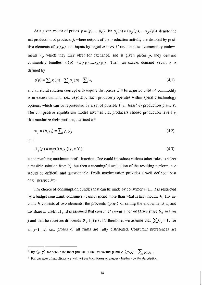
At a given vector of prices p = (p, , ... ,pK ) , let y, (p) = (y (p), ... , y jK (p)) denote the
net production of producer j, where outputs of the production activity are denoted by posi-
tive elements of yj(p) and inputs by negative ones. Consumers own commodity endow-
ments wi, which they may offer for exchange, and at given prices p, they demand
commodity bundles xi (p) = (x,, (p), ... ,x, (p)) . Then, an excess demand vector z is
defined by
and a natural solution concept is to require that prices will be adjusted until no commodity
is in excess demand, i.e., z(p) 10. Each producer j operates within specific technology
options, which can be represented by a set of possible (i.e., feasible) production plans 5. The competitive equilibrium model assumes that producers choose production levels yj
that maximize their profit n j , defined as3
and
is the resulting maximum profit function. One could introduce various other rules to select
a feasible solution from 5 , but then a meaningful evaluation of the resulting performance
would be difficult and questionable. Profit maximization provides a well defined 'best
case' perspective.
The choice of consumption bundles that can be made by consumer i=1, ..., I is restricted
by a budget constraint: consumer i cannot spend more than what is his4 income hi. His in-
come hi consists of two elements: the proceeds (p,w,) of selling the endowments wi and
his share in profit n,. It is assumed that consumer i owns a non-negative share 9;j in firm
j and that he receives dividends 9,n (p ) . Furthermore, we assume that x.9, = 1 , for
all j=l,..,J, i.e., profits of all firms are fully distributed. Consumer preferences are
By (p, y) we denote the inner product of the two vectors p and y: (p, y) = xk pk yk . For the sake of simplicity we will not use both forms of gender - hislher - in the description.
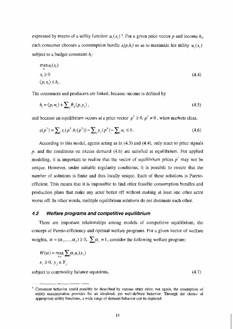
expressed by means of a utility function ui (xi) 5 . For a given price vector p and income hi,
each consumer chooses a consumption bundle xi(p,hi) so as to maximize his utility ui(xi)
subject to a budget constraint hi:
max ui (xi ) xi
xi 2 0
(P , xi) 5 hi.
The consumers and producers are linked, because income is defined by
and because an equilibrium occurs at a price vector p* 2 0, p* z 0 , when markets clear,
According to this model, agents acting as in (4.3) and (4.4), only react to price signals
p, and the conditions on excess demand (4.6) are satisfied at equilibrium. For applied
modeling, it is important to realize that the vector of equilibrium prices p* may not be
unique. However, under suitable regularity conditions, it is possible to ensure that the
number of solutions is finite and thus locally unique. Each of these solutions is Pareto-
efficient. This means that it is impossible to find other feasible consumption bundles and
production plans that make any actor better off without making at least one other actor
worse off. In other words, multiple equilibrium solutions do not dominate each other.
4.2 Welfare programs and competitive equilibrium
There are important relationships among models of competitive equilibrium, the
concept of Pareto-efficiency and optimal welfare programs. For a given vector of welfare
weights, a = ( a ,,... ,a , ) 2 0, c.ai = 1, consider the following welfare program:
W(a) = maxx ,a i u i ( x i ) x SY
x i 2 0 , y j E Y j
subject to commodity balance equations,
Consumer behavior could possibly be described by various other rules; but again, the assumption of utility maximization provides for an idealized, yet well-defined behavior. Through the choice of appropriate utility functions, a wide range of demand behavior can be depicted.

(shadow price p).
We note that the solution of such a welfare program is meaningful without any
specific assumptions on the specification of utility functions or production sets. In the
general case, however, a central coordination of agents may be required to achieve the
welfare maximum. When meeting some additional properties, the welfare program can be
decentralized and the solution be calculated by competitive equilibrium. Assume that the
production set q allows for inaction, i.e., 0 E ', and is compact and convex. Furthermore,
assume that the utility functions ui are continuous, concave, increasing, and that ui (0) = 0
and x . w i > 0. Then, according to the Second Welfare Theorem (for instance, see
Gunning and Keyzer 1995), for every vector of welfare weights a there exists a
corresponding vector of transfers among consumers, bi , with x , b i = 0 , such that an
optimal solution of the welfare program, say x* and y*, is equivalent to a competitive
equilibrium with transfers bi among consumers. With transfers, incomes, and hence budget
constraints, are modified to:
In this way, a competitive equilibrium with transfers can account for equity considera-
tions and is Pareto-efficient at the same time. The transfers between consumers are also
referred to as lump-sum subsidies (when positive) or lump-sum taxes (when negative).
Also, any competitive equilibrium without transfers is Pareto-efficient and corresponds to
a choice of welfare weights a > 0 such that b; = 0 , i = 1 ,...,I.
When demand is described at an aggregate, say national, level without specifying in-
come distribution, the equilibrium model is reduced to the single consumer case as is often
assumed in applied models. Then, if there is only one consumer, the optimum of a convex
welfare program is a competitive equilibrium solution (since transfers are necessarily
zero), and computing an equilibrium solution is achieved by analyzing and solving a
convex optimization problem.
This brief discussion shows that for given ownership of endowments and for fixed
shares in firms, a competitive equilibrium without transfers will be Pareto-efficient but
may be considered unacceptable from an equity perspective. A competitive equilibrium

with transfers accounts for equity considerations without losing efficiency. Furthermore,
let us notice that the Pareto-optimal outcomes of welfare maximization and competitive
equilibrium models suggest that these concepts are socially desirable. Even if individual
producers become sufficiently powerful to affect prices, they would not be able to
improve upon the Pareto-optimal outcome of a competitive equilibrium (albeit they will
most likely improve their own welfare). Of course, multiple Pareto-optimal outcomes will
in general be different in various respects, for example, equity considerations. Welfare
analysis aims at the consideration of such issues.
4.3 Incorporating policy measures in welfare programs
Traditionally, general equilibrium models have dealt with cases where all commodi-
ties, goods and factors, are exchanged on competitive markets. Of course, this assumption
is not always valid, especially when considering environmental resources. In this case we
must include a central agency in the model, for instance government, responsible for
optimally setting levels of taxes, subsidies, norms (e.g., environmental standards and
regulations) and other policy measures. From a formal point of view this case can again be
treated within the general equilibrium framework. The government can be considered as
an additional actor: it may own endowments and receives income from taxes and tariffs. It
may own firms, but these firms should operate like private firms (i.e., be profit
maximizing), not as price-setters. The government has the authority to impose taxes,
provide subsidies and administrate lump-sum transfers. The government uses its income to
finance public consumption and investment, and to redistribute the proceeds from taxation
among producers and consumers. Let the consumption bundle of the government be
denoted by xg and let the preferences of the government be described by a utility function
uR(xR). Like other actors, government maximizes its objective function subject to a budget
constraint.
Let us now consider some possible government policies. For example, when consider-
ing a commodity tax (or subsidy) at rate zk , the consumer price p,' of commodity k is
related to the clearing price p, , i.e., to the variable associated with the market clearing
conditions, according to:

where the rate zk is positive for a tax and negative in case of subsidies. The budget con-
straint of consumer i thus reads:
~ k ( ~ + ~ k ) ~ k ~ i k <hi (4.10)
where income hi is defined as in (4.8).
Of course, taxes can also be made consumer or producer specific, e.g., to assist a spe-
cific group of producers such as farmers. In practice, various measures like taxes,
subsidies and quotas have been introduced by governments to support specific groups of
agents by means of price supports rather than by direct income transfers, or to protect
particular activities, say growing of rice, from the effects of international competition.
Taxes and subsidies, in general, discourage or promote the production and use of specific
commodities. Governments use the proceeds of taxes, T = xkrkpkxx , , to finance
public consumption xg, price subsidies (when zk<O), and lump-sum transfers b,. Tax-ridden
prices pc can also be generated directly by a welfare program (e.g., see Ginsburgh and
Keyzer (forthcoming), Fischer et al. 1988):
w ( a ) = max C , a , u , (xi ) - (5, x) X,Y
~ ~ 5 2 0 , x i 2 0 , i = l , ... , I , y j e 5 , j = l ,.,., J
subject to
x - C y j I < C i w i (shadow price p)
~ 2 C . x ~ (shadow price pc)
where we define a vector of nominal taxes, 5 = (5, , . . . , t ,) , by a feedback relationship, so
as to obtain in equilibrium taxes 5, = z k p k , where zk is fixed. Then, the welfare weights
a, are set in such a way that every consumer, private or public, meets his budget
constraint:
Any equilibrium solution with taxes will be optimal for the welfare program. Note that
indirect taxes on producers can be treated in the same way. However, from (4.1 1) it is
clear that any such taxes and subsidies will hamper efficiency of resource allocation and
thus reduce welfare.
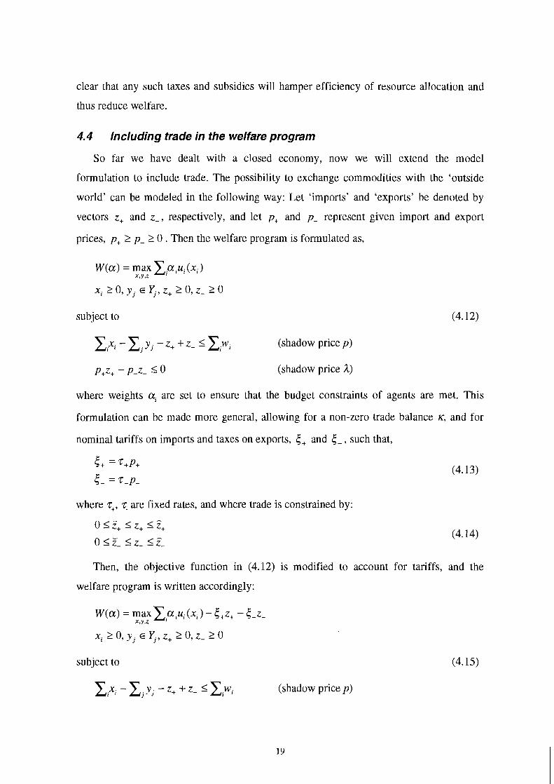
4.4 Including trade in the welfare program
So far we have dealt with a closed economy, now we will extend the model
formulation to include trade. The possibility to exchange commodities with the 'outside
world' can be modeled in the following way: Let 'imports' and 'exports' be denoted by
vectors z+ and z-, respectively, and let p+ and p- represent given import and export
prices, p+ 2 p- 2 0 . Then the welfare program is formulated as,
W(a) = max x , a i u i ( x i ) X . Y . 2 '
subject to
x i x i - ~ y j J -z+ +Z- 5 x i w i (shadow price p)
p+z+ - p-Z- 5 0 (shadow price a)
where weights ai are set to ensure that the budget constraints of agents are met. This
formulation can be made more general, allowing for a non-zero trade balance K, and for
nominal tariffs on imports and taxes on exports, 5, and 5-, such that,
where z+, 7 are fixed rates, and where trade is constrained by:
Then, the objective function in (4.12) is modified to account for tariffs, and the
welfare program is written accordingly:
subject to
(shadow price p)
(shadow price A)
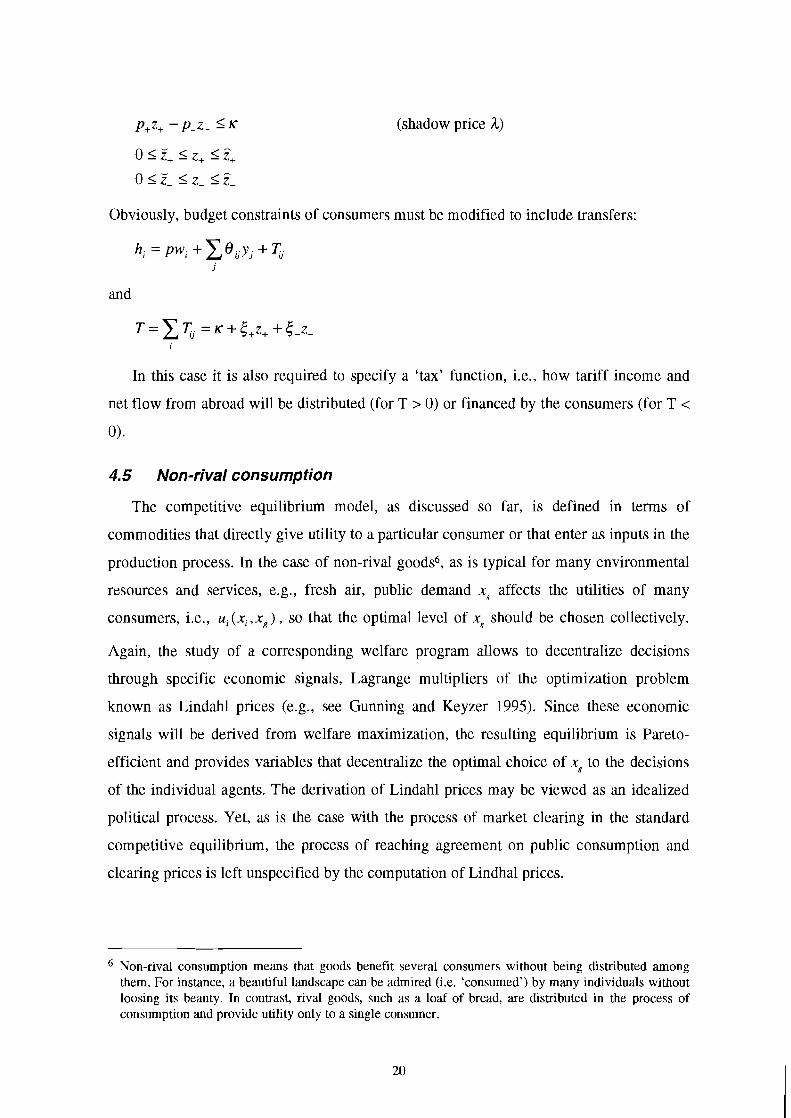
Obviously, budget constraints of consumers must be modified to include transfers:
and
In this case it is also required to specify a 'tax' function, i.e., how tariff income and
net flow from abroad will be distributed (for T > 0) or financed by the consumers (for T <
0).
4.5 Non-rival consumption
The competitive equilibrium model, as discussed so far, is defined in terms of
commodities that directly give utility to a particular consumer or that enter as inputs in the
production process. In the case of non-rival goods6, as is typical for many environmental
resources and services, e.g., fresh air, public demand xg affects the utilities of many
consumers, i.e., ui(xi,x,) , so that the optimal level of xg should be chosen collectively.
Again, the study of a corresponding welfare program allows to decentralize decisions
through specific economic signals, Lagrange multipliers of the optimization problem
known as Lindahl prices (e.g., see Gunning and Keyzer 1995). Since these economic
signals will be derived from welfare maximization, the resulting equilibrium is Pareto-
efficient and provides variables that decentralize the optimal choice of xg to the decisions
of the individual agents. The derivation of Lindahl prices may be viewed as an idealized
political process. Yet, as is the case with the process of market clearing in the standard
competitive equilibrium, the process of reaching agreement on public consumption and
clearing prices is left unspecified by the computation of Lindhal prices.
Non-rival consumption means that goods benefit several consumers without being distributed among them. For instance, a beautiful landscape can be admired (i.e. 'consumed') by many individuals without loosing its beauty. In contrast, rival goods, such as a loaf of bread, are distributed in the process of consumption and provide utility only to a single consumer.

5. Spatial aspects of modeling land-use and land-cover change
In the economic framework being developed in the LUC project we represent human
activity as variations of three types of economic agents: consumers (e.g., rural and urban
households), producers (e.g., firms, representative farms, forestry sector enterprises) and
government. Of course, the representation of individual consumers and producers is an im-
possible task; rather, we describe representative 'homogenous' groups of consumers and
producers, termed agents of the model. As will be elaborated later on, a 'consumer' may
be a segment of the population, a social class, national or local governments, an
international agency, or a foreign economic agent with demand for export commodities.
Consumers can be differentiated with regard to geographic location, level and source of
income, habits, and value system. Differentiation into income strata is relevant to
analyzing social impacts, for instance of poverty and hunger, and hence of economic
hardship which may lead to exploitation of marginal areas and environmental degradation.
Classes of consumers represent specific segments of the population and are
characterized in terms of their preferences and budgets. At minimum, rural and urban
households in each geographical unit will be distinguished in the LUC model, and perhaps
be organized into different income strata. Consumer preferences will be expressed through
demand systems using nested expenditure categories (see Section 9, Table 9. I), with broad
commodity groups at the highest level, including foods, wood products, energy, industrial
goods, housing, services, and recreation. Expenditure categories with a strong link to land
use must be further subdivided. For instance, in the food category we distinguish con-
sumption of different crop commodities (cereals, root crops, vegetable oils, etc.) and live-
stock products (meat and milk).
Similarly, producers are grouped according to distinguishing characteristics, such as
sector of the economy, level of management and technology, or kind and adequacy of
resource endowment.
5.1 Defining the spatial representation
A model for studying land-use and land-cover changes must be geographically
explicit. The geographical representation should allow for sufficient differentiation of

geobio-physical determinants of land productivity, and hence of land use, such as climatic
conditions, soil characteristics, and landform (i.e., physiography, relief intensity, slope,
aspect). Representation of social, economic and political organization, e.g., national and
regional administrative boundaries, is essential as well. To reflect, yet structure, the wide
range of heterogeneity of the real-world system it is helpful to consider the concept of
compartments in the LUC model.
The approach we adopt is based on subdividing the study region into compartments,
i.e. sub-regions. Actors and processes in each compartment ideally are to be represented by
a stochastic and dynamic model of the kind discussed in the later sections of this paper.
Depending on scale, a compartment may correspond to a collection of farms, to a
watershed, a zone within a country, or a group of provinces. Compartments are defined to
reflect structured entities, i.e., sub-systems, of the broader region under consideration and
their economic and other interactions. Since the kind and degree of organization of social
and economic systems may change over time, as may the biogeophysical properties of
land, the specification of compartments must avoid being geographically static. In applied
studies such as the LUC project, modeling is usually accomplished on the basis of spatial
data sets organized on rectangular grids. Compartments are defined as collections of grid
cells, and can possibly vary over time. The basic level of spatial organization is thus the
grid cell. Note that areas not subject to direct human forcing, e.g., wilderness areas, form
separate compartments with land cover derived from simulated trajectories of natural
vegetation7.
The notion of a compartment, as used here, does not exclude internal heterogeneity of
certain characteristics, such as soil or landform; a compartment may itself be subdivided
into smaller homogenous land management units to form the basis for a meaningful
biogeophysical evaluations. For instance, a valley in a mountainous region that
These compartments may still impact upon agents of other compartments by providing utility (e.g., recreation, clean air, 'beautiful' landscape) or affecting joint constraints. For instance, if policy regulations demand a certain water quality in the wilderness area, then shadow prices (e.g., of environmental taxes, or of emission permits) in neighboring compartments will be affected when appropriate regional environmental constraints are imposed. In land evaluation as carried out by F A 0 and others (e.g., FAOIIIASA 1993), such basic land units have been termed agro-ecological cells. Because of scale of analysis, these cells often cannot be geo-coded precisely but are known (in a statistical sense) to represent a land quality within the geo-referenced map unit, e.g., a map unit of the FAOIUNESCO soil map.

economically depends on forestry, dairy production and tourism may become a com-
partment even though there is likely to be a large heterogeneity of resources within that
compartment, e.g., in terms of steepness of slopes, soil type and even climate zones. Land
management units within the compartment should refer to relevant combinations of such
heterogeneous attributes. Section 8 discusses the representation of land in more detail.
5.2 Organization of spatial units
Compartments will be organized hierarchically, e.g., provinces, countries, groups of
countries with formal economic and political collaboration (e.g., the European Union),
broad regions, etc. Since agents in the model are identified at the compartment level,
technological, environmental and financial constraints can be specified at various levels of
aggregation within the hierarchy. That way, much descriptive realism can be introduced
into the model specification. Decision-making can be represented at the appropriate
administrative level, and local, national, and international markets can be simulated.
Environmental constraints and mechanisms to enforce environmental agreements can be
depicted at the relevant spatial and administrative level. Thus, the proposed structure
allows for much flexibility in modeling driving forces operating at different spatial and
organizational scales.
In practice, compartments will often be derived by superimposing maps of different as-
pects of the land, e.g., administrative boundaries, social and economic organization,
climate zones, landforms, etc., and then drawing boundaries that best reflect the most
important distinctions among these map layers. Geographical information systems (GIs)
provide powerful assistance in storing and manipulating geo-referenced data. The details
of defining and characterizing compartments will, in general, vary with the purpose of a
study and the scale of the study area. In the LUC project, several geographic layers for the
continental model are being assembled at a scale of 1:4 million. Climate, landform, soil,
and vegetation maps form the backbone of the biogeophysical land characterization. The
description of compartments and their agents must refer to relevant endowments,
applicable economic and physical balance equations (like budget constraints, balance of
commodity demand and supply, or consistency of resource use and availability), with
identification of 'immobile' resources (e.g., soil, climate) of each compartment and the

'mobile' resources (e.g., labor, capital, minerals, water) which can be redistributed or
'traded'.
In the LUC model, compartments (i.e., their economic agents) interact through
commodity trade and financial markets, and flows of mobile resources. They compete for
allocation of limited public resources and foreign investment. They are jointly affected by
government policies, regulations and other regional constraints. Compartments also
interact through material transport and transboundary flows of pollutants. Human
migrants, mostly rural to urban migration, may generate demographic flows across com-
partment boundaries.
5.3 Representing commodity and resource flows
With respect to the interaction of different compartments, due consideration must be
given to an adequate representation of the physical flows of commodities in the LUC
model system. Two aspects need to be mentioned: (i) transformation of commodities
through processing when flowing from the production site, e.g., farm-gate, to the
consumer, and (ii) transportation requirements to bridge distance when flowing to markets
in different locations. For a tractable implementation, some simplifications are adopted in
both respects.
As to the transformation of commodities, one approach to dealing with processing is to
represent all levels of processed commodities separately in all markets. This would most
likely constitute a large burden to data collection, model specification and parameter
estimation. Another approach, recommended here, is to treat processed commodities as
consisting of raw materials, produced at farm-gate or forest enterprise, plus a non-
agricultural commodity which accounts for processing activities and transportation. When
the non-agriculture sector is sufficiently disaggregated in its description, these can be
separate inputs. The prices seen by consumers in different markets will therefore consist
of a raw material component, a processing margin, transportation margins, and possibly
taxes or subsidies, and tariffs. Such an approach has been applied, for instance, in Fischer
et al. (1988) and Folmer et al. (1995).
Transportation requirements, in particular, are critical since the LUC study must give
due consideration to comparative advantage among producers resulting from differences in

geographic location. Consumer prices of land-based products, i.e., of most food stuffs and
wood products, typically contain only a small raw material component. Therefore,
differences in transportation requirements related to different geographic locations will
largely determine the viability of export and import strategies. Export cropping will be
rather unlikely in remote locations. On the other hand, some land uses which might
otherwise not be competitive may become viable or even necessary because of prohibitive
transport requirements.
In the most elaborate representation of these aspects, the modeler tries to maintain
product heterogeneity with regard to a vector of physical commodity characteristics, loca-
tion of origin, and location of use. Hence, maize produced in France and used in Russia
would be listed as a separate commodity, different from maize produced in Hungary and
used in Poland. Such a treatment may be required, for instance, if one wishes to keep track
of bilateral trade flows, or of some forms of preferential trade agreements. However, such
a treatment of heterogeneity has a dire cost in terms of the number of decision variables
generated and the number of commodity balances that must be cleared. For instance, if a
model specification deals with only 25 tradable commodities and 20 regions, then in a free
routing case, i.e., when all bilateral flows are technically possible and unrestricted, the
number of trade flow variables is 20~19x25 = 9500. The situation may improve somewhat
with constrained routing. When additional information is available, e.g., indicating techni-
cal impossibility or political undesirability of trade, bounds on specific trading activities
can be set to reduce the number and limit the volume of bilateral trade flows.
For applied modeling, researchers have developed simplifying assumptions that are
geared to overcoming the difficulties of commodity heterogeneity and the associated vast
data requirements. Two methods have been widely used and are especially relevant for
consideration in the LUC project, the Armington approach and the trade-pool approach.
Following the Armington approach (Armington 1969), the modeler postulates that
sectors differentiate among imported commodities according to the country of origin, and
among domestic and imported varieties. The Armington structure has been criticized as
being unnecessarily restrictive. However, it has been widely used in world trade models,
allowing, in a straightforward manner, to combine trade in similar goods with conditions
of less-than-perfect import demands (Hertel 1995).

A common approach to reduce the complexity of a full trade matrix and to avoid pos-
sible indeterminacy of trade flows is to assume a trade pool into which all exports flow
and from which all imports originate. This approach eliminates bilateral trade flows but
allows to retain information on transportation costs as well as constraints on routes to and
from the pool. Transportation is thus interpreted as a means to homogenize commodities
that differ by location only and have identical physical characteristics otherwise
(Ginsburgh and Keyzer, forthcoming).
5.4 Implementation of the trade-pool approach
As a starting point in the LUC modeling effort, we follow the trade-pool approach and
distinguish four levels of commodity transformation: raw materials (basic products as
obtained at the production site), processed commodities in the local (regional) market,
commodities processed and transported to the national level market, and commodities
transported to and obtained from the world market. Policy measures and restrictions to
commodity flows are conceivable at all of these levels. It is important to ensure that the
commodity mapping between levels is kept consistent in both physical and value terms.
An illustration of the resulting spatial hierarchy is shown in Figure 5.1 and Figure 5.2.
Let the transformations between different commodity levels be described by matrices
T ~ , T r , T n , respectively. For instance, mapping T r is applied to convert trade flows from
national retail level zrn to regional level z r , and mapping T n to go from international
trade level znw to national retail level z" . Furthermore, let pJ ' , pr , pn , and pw , denote the
respective prices. If only transportation activities are involved, e.g., to convert from
national retail level zrn to the local retail level z r , the transformation matrix T r has a very
specific form. For instance, in the case of four retail commodities, with the third sector
providing transportation services of t,', k = 1, ..., K, units per unit of commodity k
transported, the mapping matrix becomes:

Then, the following relationships (or similar ones, depending on model specification)
between prices and physical quantities must hold for consistency of the mappings:
py = pY(I - Tn)
p: = p:(I - Tr) for exported commodities,
pf = P L ( ~ -T')
and similarly for prices of imported commodities, p+ ,
p: = p,"(I + Tn)
p: = p:(I+Tr) for imported commodities.
pi = p:(~ + T')
For physical volumes at different levels of the spatial hierarchy we obtain dual
relationships for exported and imported commodities, z- and z+ , respectively:
z> (I - Tn)zlfw z: = (I + Tn)z:"
z: = (I - Tr)zl" and z: = (I + Tr)z;
zy = (I - T"')z~. z: = (I + T')z:
The relationships in (5.5) indicate how commodities must be accounted for at different
levels of the spatial hierarchy in order to maintain consistency of physical flows. For
instance, import of commodity vector z:" from the global commodity pool will result in a
vector z: to enter the national commodity pool. Note that the T-mappings in (5.4) and
(5.5) could be differentiated according to the direction of trade, i.e., separate mappings for
exports and for imports. Figure 5.1 shows in a simplifying way how regional production,
denoted by q, gets transformed to the regional retail level, where it may be used for
consumption, d, or as intermediate production input, v, or may enter or leave stocks, s. In
the figure, the local commodity pool is linked to the national level by means of a region-
specific transformation, qh" (h referring to country index and s denoting a region within
country h), and further to the international market through a country specific mapping, ~ , h
Figure 5.2 illustrates that in this spatial hierarchy commodity flows can be limited and
prices be distorted by policy measures9.
There may also be reasons of physical infrastructure that limit commodity flows.


Figure 5.2: Spatial hierarchy in LUC modeling system

5.5 Construction of commodity balances
Figure 5.1 and the discussion in Section 5.4 have indicated the flows and processing
transformations of commodities, from the production site, e.g., farm or forest enterprise, to
the final demand destination. We have also introduced the concepts of market-clearing
conditions in Section 4 (e.g., see (4.5)). We can now construct commodity balances, at
different levels of the spatial hierarchy, which constitute fundamental relationships in
applied general equilibrium models. For this, we recapitulate the variables that enter the
commodity balances of each sub-region r:
qr vector of production in region r,
s: sales from stocks, r
s- purchases to stocks,
z: imports to sub-region r, r
Z - exports from sub-region r,
d r final consumption in sub-region r,
vr intermediate inputs in sub-region r,
i' investmentlo in sub-region r.
Then, commodity balances at sub-regional, national and world level are, respectively,
obtained as,
Commodity balance in sub-region:
qr +s: -s '+z: -z ! 2 d ' + v r + i r
National commodity balance:
Consistency of trade within country:
Consistency of global trade:
1°Note that investment (as all other variables) refers to physical commodities, not value terms.
30 ,

where variables z:, zy , zi, zr and z:, z: , zlf , z_"" are related as in (5.5). Furthermore, we
may impose specific limits on commodity flows at the country or regional level by
requiring that (5.10) holds in addition to (5.6) - (5.9):

6. Temporal aspects of land-use change
A main task of the LUC project is to study the sensitivity of land-use and land-cover
change dynamics to various policies, behavioral assumptions, demographic and socio-
economic developments, and to environmental conditions. Hence, dynamics is a critical
issue in the modeling effort. The time-span of the analysis covers the period from 1990 to
2050, which is subdivided into 5-year intervals. Thus, the model is of discrete time with
thirteen time steps, t = 1 ,..., 1 3. The initial step, with t = 1, refers to year 1990 and the final
step, t = 13, refers to the end of the model horizon, i.e., to the beginning of year 2050.
We turn now to discussing temporal aspects of modeling consumer and producer
behavior in the LUC model. For this we discuss the role of model-endogenous and model-
exogenous dynamics and introduce intertemporal specifications of consumers' utility
function and the producers' profit function. The aim is to describe how variables of
interest change over time. There are many factors that may cause such changes. We group
them into two sets: factors exogenous to the welfare analysis and factors endogenous in it.
For instance, time-dependent exogenous factors include variables such as parameters that
describe the shift in technology, e.g., of production functions, changes in characteristics of
agents, e.g., changes in life-styles expressed through shifts in parameters and functional
forms of the demand system, or changes in policy variables, like trajectories of tax levels.
Exogenous dynamic factors are easily implemented, by allowing for time-dependent
functions in the model. Their introduction does not lead to any essential methodological
complications and can be dealt with effectively by simple extensions of the static
framework (see Section 4) by means of recursive dynamic simulation. This involves
computing a sequence of single-period equilibrium solutions for periods t = 1,2, ... which
are related through the updating of some parameters and exogenous variables.
When dynamics depend on endogenous factors, such as on allocation decisions of
consumers (e.g., allocation of income to savings and consumption) and of producers (e.g.,
decisions on investment and resource use), a static model formulation is clearly
insufficient. This section mainly serves the discussion of endogenous dynamics in the
LUC model.

6.1 lntertemporal welfare analysis
Ideally, intertemporal welfare analysis should start from an infinite time-horizon. Two
conceptually different approaches exist to implement infinite-horizon models and to
perform such an analysis:
(i) To deal with a finite number of infinitely lived agents. For example, the initial
population of a geographical unit and its descendants can be interpreted in this
way. This kind of representation is called dynastic model. The basic mechanism to
deal with intertemporal aspects of consumer decisions is to include so-called time-
recursive consumer preferences. Each agent's (i.e., each dynasty's) well-being, uf ,
in period t, is described as depending on current consumption, x f , as well as next
period's well-being, u j'l , through:
(ii) To consider an infinite number of generations of finitely-lived agents. Each
generation lives (at least) two time periods, e.g., labeled 'young' and 'old7. Also,
generations overlap, i.e., the 'old7 of generation one live together with the 'young'
of generation two, etc. Because of this feature, such models are termed overlapping
generations models.
Various specifications of both types of models are discussed in Gunning and Keyzer
(1995) and Ginsburgh and Keyzer (forthcoming). In the LUC project, we start from the
dynastic model specification. It is generally impossible to solve numerically a model with
an infinite number of unknown variables or equations, as occur in infinite-horizon dynastic
and overlapping generations models. Infinite-horizon models and the proposed solution
techniques suffer also from various other theoretical and practical problems (e.g., as
discussed in Gunning and Keyzer 1995). Therefore, in the LUC project we aim to
implement a finite-horizon approximation of the infinite problem.
6.2 T-period general equilibrium models
A competitive general equilibrium setup where agents decide on current and future
periods over a finite time horizon, t = 1, ..., T, is referred to as T-period competitive
equilibrium. A critical disadvantage of finite horizon models is that the state of the system
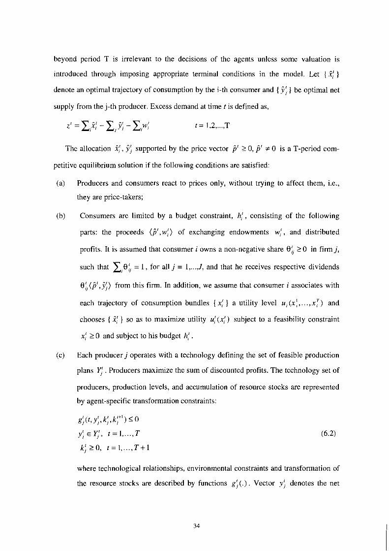
beyond period T is irrelevant to the decisions of the agents unless some valuation is
introduced through imposing appropriate terminal conditions in the model. Let { if )
denote an optimal trajectory of consumption by the i-th consumer and { j j ) be optimal net
supply from the j-th producer. Excess demand at time t is defined as,
The allocation i f , yf supported by the price vector j' 2 0, j' # 0 is a T-period com-
petitive equilibrium solution if the following conditions are satisfied:
(a) Producers and consumers react to prices only, without trying to affect them, i.e.,
they are price-takers;
(b) Consumers are limited by a budget constraint, hi', consisting of the following
parts: the proceeds ( i f , wf) of exchanging endowments wlf , and distributed
profits. It is assumed that consumer i owns a non-negative share 8; 2 0 in firm j,
such that X . 0 ; = 1, for all j = 1, ..., J, and that he receives respective dividends
8; ( j t , j j ) from this firm. In addition, we assume that consumer i associates with
each trajectory of consumption bundles { xlr ) a utility level u, (xl, . . . , x') and
chooses { ill ) so as to maximize utility u1!(xlt) subject to a feasibility constraint
x,! 2 0 and subject to his budget hi'.
(c) Each producer j operates with a technology defining the set of feasible production
plans qf . Producers maximize the sum of discounted profits. The technology set of
producers, production levels, and accumulation of resource stocks are represented
by agent-specific transformation constraints:
where technological relationships, environmental constraints and transformation of
the resource stocks are described by functions gi ( . ) . Vector y f denotes the net

supply of commodities to the market, kf is the stock of resources (including capi-
tal, labor, land, etc.). Vector k:" is the stock of resources that, given y: and kf ,
will be made available in period t+l. Some of the components of the stock of re-
sources will be produced in period t or may use inputs of stock kf , others may
grow or deplete at a natural rate or be generated by production processes.
There may also be joint constraints on total outputs from all producers j = 1 ,..., J,
e.g., on total emissions of CO,, or on deposition of SO, at a given receptor. Note
that such constraints may be decentralized through implementation of 'production'
permits, possibly tradable permits that can be exchanged between producers.
When dealing with a finite number of time periods T, it is critical to include
appropriate terminal conditions. These may significantly affect the trajectories of
allocations until period T.
(d) Markets are in equilibrium for all periods t = 1, ..., T:
An important aspect of T-period competitive equilibrium models is intertemporal
Pareto-efficiency, i.e., they generate trajectories of allocations such that no agent can be
made better off without somebody else losing. As discussed in Section 4 for static models,
an equivalent intertemporal welfare program can be formulated as maximization of:
x; 20, y ; E Y,!
subject to constraints for periods t = 1, ...,T:

Taxes and international trade can easily be incorporated within this dynamic model,
trade balances can be written as an intertemporal constraint:
where K is the overall trade deficit of a compartment, and other trade-related variables are
defined as in previous sections. Furthermore, the trade balance can also be written in the
form of a sequence of constraints rather than as an aggregate constraint:
where K ' is the deficit in any particular period t, possibly with an additional requirement,
equivalent to (6.5):
Examule 6.1: Let us consider two simple examples of actor-based intertemporal decision
plans. For instance, using the notation of the previous sections, we can describe a
smallholder subsistence agricultural system by an intertemporal maximization problem:
max u(xl,. . . ,xT) Y -1
xt S Y t
g(t,y', kt , kH1) S O
x ' 2 0 , t = l , ..., T
where u(.) denotes the utility function of the farm household, y is net farm output, x is a
vector of final consumption, and k refers to the quality and quantity of resource stocks. In
this specification, the subsistence household is assumed to maximize discounted utility
over the entire period, t = 1, ..., T. Consumption is determined by net farm output, i.e.,
production less intermediate consumption (seed, feed, waste). Production y' is constrained
by the available technology and resource endowment kt and the need to maintain resources
k"', as specified in transformation function g(.). Note that in this formulation the optimal
decision of the farm household is independent of markets and government-imposed fi-
nancial measures, such as taxes or price subsidies. Government can influence optimal
decisions under subsistence farming only if it is able to affect the technology set or to
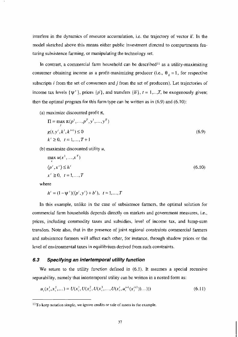
interfere in the dynamics of resource accumulation, i.e. the trajectory of vector kr. In the
model sketched above this means either public investment directed to compartments fea-
turing subsistence farming, or manipulating the technology set.
In contrast, a commercial farm household can be described" as a utility-maximizing
consumer obtaining income as a profit-maximizing producer (i.e., 8 ii = 1, for respective
subscripts i from the set of consumers and j from the set of producers). Let trajectories of
income tax levels { y~ ' }, prices {p'), and transfers {b'), t = 1 ,..., T, be exogenously given;
then the optimal program for this farm type can be written as in (6.9) and (6.10):
(a) maximize discounted profit n, T 1 II = max x ( ~ ' , . . . , p ,y ,..., yT)
(b) maximize discounted utility u,
max u(xl , . . . ,x T, X
(p l ,x ' ) l h'
x ' 20 , t = l , ..., T
where
h '=( l -y~ ' ) ( (p ' ,y ' )+b ' ) , t=1, ..., T
In this example, unlike in the case of subsistence farmers, the optimal solution for
commercial farm households depends directly on markets and government measures, i.e.,
prices, including commodity taxes and subsidies, level of income tax, and lump-sum
transfers. Note also, that in the presence of joint regional constraints commercial farmers
and subsistence farmers will affect each other, for instance, through shadow prices or the
level of environmental taxes in equilibrium derived from such constraints.
6.3 Specifying an intertemporal utility function
We return to the utility function defined in (6.1). It assumes a special recursive
separability, namely that intertemporal utility can be written in a nested form as:
ui (x :. , x; , . . . ) = U(x j , ~ ( x f , U(x:, . . . , ~ ( x f , uf" (x;' )). . . ))) (6.11)
"To keep notation simple, we ignore credits or sale of assets in the example.
37
This representation is very practical for implementation as it allows to concentrate on a
series of linked single-period sub-problems. A special form of the intertemporal utility
function commonly used in applied studies is obtained from (6.1 1) under the simplifying
assumption that the terms of consumers' utility involving current consumption and utility
in future periods are separable and linearly related, such that:
If 0 < y < 1 is constant over time12, (6.1 1) simply becomes
This specification assumes that past consumption levels influence future ones only via the
budget constraint, and that utility in period t is not affected by consumption in earlier
periods. More complicated forms of the intertemporal utility function can cope with these
restrictions.
6.4 Population dynamics
A third type of dynamics relates to the changing number and composition of agents in
the LUC model. We adopt the assumption that the agents in the model fall within
homogenous groups. To avoid theoretical problems of indivisibility, we further require
these homogenous groups to be relatively large. For instance, we assume the initial
population of each geographical unit to form such homogenous groups. Over time, the size
of each group is adjusted through two mechanisms: (i) demography of births and deaths,
and (ii) transition and migration between groups, e.g., rural to urban, or between
geographic units.
This is important, since one fundamental endowment of each group of agents, namely
labor, depends on the number of group members. Apart from having their endowments
move among locations and social classes, consumers changing group membership will
usually also change life-styles and demographic characteristics. When taking group
membership into account it is convenient to assume that utility functions are separable
over time and by social groups to which an individual may belong, and to define the well-
l 2 In this case is usually interpreted as discount factor.
3 8

being of each homogenous group i in terms of per capita utility multiplied by the number
of members in each group, i.e.,
where nf represents the number of members in group i in period t, xf is total consumption
of group i, and u f ( x : / nf) denotes utility of an individual in period t being member of
group i. In the LUC project, we will start by describing demographic transitions and
migration, i.e., trajectories of nf , exogenously13. However, the LUC approach is flexible
and allows to endogenize group membership later on, for instance, making it dependent on
relative wages among sectors of the economy as well as among geographical units.
6.5 Recursive dynamic equilibrium models
When assuming that agents have complete and perfect foresight, the solution of the
welfare program provides best-case Pareto-efficient trajectories of future development.
Myopic models, e.g., recursive dynamic equilibrium models, are easier to calibrate and
solve than T-period optimization models. However, their solution path is driven by
expectations and, in general, intertemporal efficiency of allocations is lost. In recursive
dynamic equilibrium modelsI4, agents use only expectations of future prices instead of
prices derived from intertemporal optimization and market clearing. Since there exist
infinite possibilities to choose expectations, the meaning and relevance of simulation
results from such models can be difficult to evaluate. The expectation functions can
depend on past and current prices and other variables, but not on future prices and
allocations. Also, consumers are assumed to form expectations on the dividends of future
periods. As to equilibrium conditions of recursive dynamic models, it is only required that
markets in current period t are cleared.
When building applied models they are often used for scenario analysis. Usually a ref-
erence solution is computed; then some parameters or exogenous assumptions are
changed, a new solution is calculated and this is compared with the reference solution.
I 3 ~ o t e that this will still affect inter-temporal allocations and efficiency. Thus, it cannot be dealt with in a recursive dynamic structure.
I 4 ~ n example of an applied recursive dynamic equilibrium model is IIASA's Basic Linked System (see Fischer et al. 1988).

Such comparative analysis, of course, can use various types of dynamic equilibrium
models, both T-period and recursive dynamic.
6.6. The welfare approach
The formulation of a welfare program is the conceptual centerpiece of the LUC
modeling activity. Therefore, we recapitulate the main features that were elaborated in
section 4 and throughout this section. The welfare program is written as an optimization
problem that maximizes the weighted sum of the utilities of the participants, i.e., the
consumers. There are four types of constraints to be specified in a welfare program:
(i) The utility constraint which specifies how the utility of a given group i of consumers
in period t depends on its consumption in that period as well as on its utility in the
next period. This is a characterization of the preferences of every group.
(ii) The transformation constraints describe the set of net supplies in period t and
resources in period t+l that are feasible at the given level of resources in period t.
This is a characterization of the technology of the economy, i.e., of its capacity to
produce commodities by means of produced commodities, labor and natural
resources. All the resource dynamics are part of this set of constraints. For example,
if there is a given stock of trees in the forest and some are cut and sold, this cutting
will together with replanting determine the stock of trees in the next period. If there is
no replanting and the cleared land is allocated to agriculture, there will also be a
change in the stocks of land: a reduction in the area under forest and an increase in
the agricultural land of a particular type. In the LUC project, a substantial part of the
data collection and analysis is being devoted to adequately specifying this set of
constraints describing the technology and resource dynamics that govern the main
land-based sectors of the economy, agriculture and forestry.
(iii) The commodity balance: for every commodity, the net demand by the consumers
cannot exceed the net supply that is feasible in the transformation constraint and from
trading.
(iv) Stock consistency: for every resource, the level used in period t+l should not exceed
the level carried over from period t.
A welfare program may look like a central plan that would be implemented in a
command economy. Clearly, this is not our aim. On the contrary, one of the main
advantages of the welfare approach is that it has a clear interpretation as a decentralized
model in which every agent can decide for himself. This decentralized model has the
following structure:
(v) Every consumer maximizes his own utility, subject to a budget constraint that spans
the time-horizon of the model.
(vi) Every producer maximizes his own profits, subject to his technology constraint.
(vii) Commodity markets clear (the equivalent of (iii) of the welfare program above).
(viii) Resource utilization matches resource availability (as in (iv) above).
Hence, the welfare program defines a standard competitive model, in which the
consumers, i.e., in the simplest case the regions in the model, own the commodities and
exchange these on markets, at prices that are taken as given by every agent in (v) and (vi)
and set so as to ensure that (vii) and (viii) hold. A mathematical description of this model
is given in the Appendix. We note that although we use the term 'competitive', one may
expect that several biophysical relations will possess technical characteristics which rule
out decentralization through prices or taxes and will require quantity rationing by a central
agency, the government, due to the non-convexity of the relationships. These issues will
have to be addressed and decided upon later as experts in the LUC team will submit their
proposed specifications on specific issues.
It is important to recall that the welfare program and its decentralized competitive
equivalent are normative with respect to the institutions. Private ownership and the
existence of all markets is a requirement for decentralization, not necessarily a description
of present-day reality in all parts of Eurasia. To derive non-ideal scenarios, distortions will
be incorporated in the welfare program and its decentralized counterpart. The realities of
present-day economies and societies will be approximated through additional distortion
terms in the objective function, e.g., such as discussed in Section 4.3 and 4.4, and through
additional sets of constraints.

7. Modeling the dynamics of resource stocks
Studying global change generally involves dealing with long-term phenomena, i.e.,
projections of economic and natural processes into the second half of the next century.
Under such premises the explicit description of resource accumulation processes becomes
important, because feedbacks and cumulative impacts (such as soil erosion over an
extended period) on the productivity of land could be essential.
7.1 Production activities and resource dynamics
Modeling production activities relevant to land-use and land-cover change in a way
that takes into account both the environmental as well as socio-economic conditions and
changes is a challenging and ambitious task. The aim of the production component of the
LUC model is to depict spatial and intertemporal allocation of land to various regional ac-
tivities, such as crop agriculture, livestock grazing, forestry, energy production and
mining, settlements and infrastructure, manufacturing, recreation and nature reserves.
The LUC model must allow integration of information from biogeophysical and bio-
geochemical process models with the economic model. This requires careful selection and
definition of compatible variables among the modeling components, as well as appropriate
temporal and spatial scales. Emphasis is placed on consistent methods of linking, not
merely technical feasibility. This involves far more than bringing various equations into a
single computer program.
Land-cover change under near natural conditions (i.e., without significant human influ-
ence) can be estimated from modeling vegetation under various projections of biogeo-
chemical processes of the Earth's system, and in particular of the climate system. Although
such an estimation is complex by itself and involves partly unresolved scientific issues, it
is nevertheless conceptually much simpler than projecting land-cover change managed by
human agents. Transformations possible under intensively managed land uses are con-
strained by natural conditions, but are highly dependent on technological development,
economic conditions, and demographic trends. This relates to intensification of production
systems within major land-use classes (especially agriculture), and also to conversion of
major land uses (e.g., conversion of arable land to non-agricultural purposes). The goal of
the supply component of the LUC model is to simulate producer responses under a wide

range of situations and policies. Where possible, historical data and statistical analyses will
be used to derive parameter estimates and to validate functional relationships.
The production component of the LUC model includes processes of resource
accumulation and degradation, feedbacks and cumulative impacts on land productivity. The
term 'resource' 'is used here in a general sense. Resources include human resources (e.g.,
with attributes such as population number, distribution, age structure, migration flows,
fertility, skill level, etc.), renewable and non-renewable natural resources (e.g., soils,
minerals, water, air), biological resources (e.g., biodiversity), and economic resources (e.g.,
capital stocks and machinery). The model will include both accumulation and degradation
processes. The latter encompass physical degradation (e.g., soil erosion, degradation of soil
structure, change in level of groundwater table) and chemical degradation (e.g., acidification,
salinization, toxification of soils; depletion of the ozone layer; nitrification of groundwater).
The model is solved for a sequence of time periods. Capital and environmental stocks
in the current period serve as inputs in the production process. Net supplies of consumer
goods and of stock levels at the beginning of the subsequent period are the results of pro-
duction and investment activities. Hence, environmental resources enter as inputs into
production and are, at the same time, affected by these production processes. In this
context, pollution is represented as a use of resources, e.g., of clean air. Production
activities are specified in terms of quantity and quality of relevant resources. By explicitly
dealing with resource accumulation, feedback mechanisms that act slowly on long time-
scales (e.g., soil erosion, aquifer depletion) can be represented.
However, the quality of environmental resources not only affects production processes.
It also has an effect on the well-being of the population: directly, through health effects of,
say a reduction in the ozone layer, or indirectly because consumers may care about the
well-being of future generations. We represent such collective dependency on the status of
the environment as non-rival consumption. As indicated in Section 4.5, elements of the
resource stock representing non-rival goods are not distributed among consumers but
many consumers may benefit from them at the same time. For implementation in the
model, health effects caused by global change and influenced - positively or negatively -
by land-cover change can be treated in two ways. First, they can be included in the utility
function of consumers and thus be valued. Secondly, they can be handled by means of
constraints on production, e.g., by enforcing environmental quality standards or by issuing
pollution permits. Since the latter is more easy to implement, we will begin in the LUC
model with including environmental constraints linked to land-use types (see Section 8),
and we will explore the possibility to include some of health effects in the utility function
of consumers.
7.2 Resource accumulation and degradation
In the LUC model, commodity supply in each compartment is generated by a number
of producers, indexed j = 1, ..., J. Production requires various inputs, goods and factors,
such as capital K,, labor L,, energy E, input materials M, and sector-specific resources A,,
e.g., land and water. Both energy and material inputs are aggregates of intermediate goods
which in turn may be aggregates of imported and domestic commodities. The outputs also
depend on management, like the level of mechanization, or technological progress. The
specification of production from land-based sectors of the economy as a function of the
extended resource vector k, = (K,, L,, E,, M,, A,) is a major task of the LUC project. The
model should represent present and anticipated practices and conditions in the study
region.
There are several methodological difficulties to be resolved. First, biological and
biophysical relations that are often represented through complex computer simulation
programs, e.g., crop yields derived from dynamic process models, have to be given a more
convenient, formal mathematical specification. Secondly, substitution effects between
variables that are commonly treated in isolation have to be specified explicitly. Finally,
formal estimation methods are needed to quantify and test the validity of the functional
relationships in a spatial setting. This requires the application and perhaps a further
elaboration of statistical methods, for instance, co-kriging methods.
Producers, e.g., decision-makers of representative farm types, are described as dy-
namic systems in terms of objectives, natural production conditions (climate, soils,
landform), endowments, resource accumulation, and relevant constraints (technology, re-
sources, input use, capital, environment, etc.). In a formal mathematical way, farm pro-

duction options and impacts on resource stocks can be described by a transformation
vector-function g(. )I5,
where t refers to time, y denotes net output, and k denotes stocks of resources, such as land
types, capital, labor, etc. In practice, vector function g( . ) will be used to specify a set of
simultaneous (possibly non-linear) equations and inequalities, to describe a feasible set of
production activities. In general, function g(.j is also affected by uncontrolled, stochastic
variables; which are discussed in Section 10.
For instance, the capital stock K, of producer j changes according to investment Ij and
the rate of capital depreciation tij:
where KJ is the initial capital stock. Of course, there may be many ways of choosing input
variables (in this example investment J ) , such as empirically derived choices or rule-based
schemes. However, profit maximization leads to efficiency and can thus provide a
reference trajectory of development. In the normative approach, each producer chooses
trajectories of inputs, LJ, E;, Mf,A f and I f , so as to maximize discounted profits.
7.3 Resource migration
The dynamics of resource accumulation and depletion becomes more complicated in
the case of multiple resources and many competing production activities in each compart-
ment. Let us define the vector of available resources in the c-th compartment of the region,
c = 1, ..., C, at time t by kf = (K:, LL, Ef, Mf,Af) 16. In a spatial context it is important to
consider also the flow of resources between compartments. Let us denote the outflow (or
'export') of resources from compartment c to another compartment h by vector rc', 2 0 and
inflow (or 'import') of mobile resources from compartment h into compartment c by vec-
tor rLc 2 0 . Assume that the flows of resources are constrained to rc; I rc', I rci; in
particular, we may also require that rci = r,', = 0 , in which case no migration of resources
15we note that the transformation function, i.e., the description of technology and resource constraints, is agent specific. The subscript denoting agents has been dropped for convenience.
1 6 ~ n l e s s explicitly mentioned, we drop the producer index j to keep notation simple.
between compartments c and h would occur. The total net migration of resources into
compartment c is obtained by summation:
h=I h= l
and thus
where k: is the initial stock of resources in compartment c. These equations can be used to
depict such diverse processes as the flows of capital, labor, or of pollutants.
7.4 Resource conversion
Land conversion within a compartment c is caused by resource allocation decisions.
Let us denote the level of conversions of the k-th resource to the m-th resource in
compartment c by c:,,,, 2 0 . Then total net conversion C;, into resource m is obtained as:
Let us note that the lower and upper bounds c,, cf used in (7.5) provide restrictions on
resource conversions. Thus, c, = cf represents fixed levels of conversion; if cf = 0 , then
no conversion is feasible. This information can be reflected in matrix form, for instance, as
is illustrated for land classes in Table 8.1, in the following section of this paper. Defining
the vector of resource conversions Cf = (Cf,, , C: , , . . . , Cf,, ) , resource accumulation
processes can be written as:
Note that the dynamics of kf must also take into account depreciation of capital
stocks, decay of natural resources, etc.; in the resource accumulation equation (7.6) given
above this is indicated by the last term, where 6: denotes a vector of depreciation rates.
A feasible allocation 0: = (Q',,) of resources among a finite number of competing ac-
tivities, indexed k = 1, ..., K, in compartment c is defined by a set of equations,
where Q:, is a vector of resources allocated to the k-th activity. In general, the choice of
variables r f , ,~;. .~,, , ,Q:., 2 0 can be modeled in a number of ways. Trajectories could be
specified as model assumptions, as part of a scenario framework, or some of the compo-
nents could be represented as stochastic processes, for instance using Markov chains. In a
fully developed normative framework the migration and conversion of resources are
deemed decision variables and can be derived from welfare maximization. A critical re-
quirement for this approach is quantitative information on the productivity of each activity
k when carried out by different producers, j = 1 ,..., J, expressed as a function of respective
resource inputs kj = (Kj, Lj, Ej, Mj, Aj).
As mentioned before, such response functions require detailed information such as
farm surveys, agronomic experimental data, as well as GIS layers of resource distribution.
We realize that a major data collection and estimation effort is required to derive reliable
estimates of production functions both for managed as well as unmanaged vegetation.
However, detailed classification of land types, of other resources, and of production units
is meaningless if the associated production functions cannot depict differences in
productivity. Once response functions are available, the model will allow the simulation of
responses to a range of policies. For example, we could evaluate the system response to
new production alternatives and technologies versus traditional practices. It is also
possible to analyze the impacts of certain restrictions on production or their relaxation, or
to investigate the consequences of improving infrastructure both within and across
compartments.
In summary, land-use models appropriate for the analysis of long-term aspects of
global change should account for changes, over time, in the level and quality of envi-
ronmental resources, socio-economic constraints, and technological conditions. While the
dynamics of resource accumulation and degradation call for a multi-period approach, the
study of vulnerability, resilience and irreversibility requires a stochastic framework. The
latter is discussed in Section 10.

8. Representing land resources and land use
The LUC project is particularly concerned with the future of land resources. Therefore,
we now extend the considerations discussed in the previous section and elaborate on how
land is adequately characterized in the economic model. We also describe how land-use
change is tracked in the model and how land-use constraints are implemented to ensure
consistency with the resource base.
8.1 Describing land resources by site classes
One can think of many diverse attributes by which to characterize land. Care should be
taken to differentiate between factors that are intrinsic to land and those that are attached
to a particular land use. For instance, soil type is an intrinsic property of a tract of land,
whereas fertilizer input is an attribute of land use. To differentiate land resources with re-
gard to land productivity in the LUC model according to physical properties, we define a
number of site classes, as, s = 1 ,..., S, in terms of intrinsic land properties. Attributes that
are considered include:
temperature regime
moisture regime
landform and slope
soil type, soil phase, soil texture, etc.
land accessibility (e.g., approximated by road density, population density, etc.)
To facilitate the creation of adequate site classes, the LUC project is currently develop-
ing several continental-scale databases in a GIs, including climatic variables, vegetation,
and land resources. Land characterization is described according to the specifications for
global and national soils and terrain digital databases (SOTER) which were recently de-
veloped (UNEP/ISSS/ISRIC/FAO 1995) and are gaining wide acceptance. In the SOTER
approach, the main differentiating criteria for land characterization are physiography,
terrain components and soil components. These criteria '... are applied in a step-by-step
manner, each step leading to a closer identification of the land area under consideration'
(UNEP/ISSS/ISRIC/FAO 1995).
8.2 Change in land characteristics over time
Land characteristics, for various reasons, may change over time. Therefore, the concept
of site classes must be dynamic and the LUC model will generate consistent trajectories of
the extents of different site classes. There are both natural processes and anthropogenic
causes that may change the properties of land, and thereby the site class to which a
particular tract of land belongs. Let us denote the transfer of land from site class s to class
w in year t by Aa:, 2 0 . Such a transfer can be caused by:
- Land improvement, e.g., through amelioration and drainage projects, because of irri-
gation projects, or by terracing. In general, land improvement requires investment,
and we indicate the cost per unit of area converted from site class s to class w, in
period t , by a cost coefficient yb, .
- Allocation of a site class s to a particular activity, e.g., land use of type h, can cause
degradation that may eventually lead to a lower site class, for instance, caused by soil
erosion.
- Climate change may imply transfer of land to a different site class as it may change,
for example, the temperature or soil moisture regime.
Extents of site classes and transfers between site classes must fulfill simple accounting
relationships:
k t s k#,s
and the cost of land transfers, AC' , is:
8.3 Defining land-use types and major land-use classes
Land use is best described in a hierarchical, nested way. At the highest level of the hi-
erarchy, we define trajectories of major land uses, A f,, , h = 1, ..., H, in each of the site
classes, at , s = 1 ,..., S. Major land uses are defined by the set {natural/unused, protected,
agriculture, grassland, forestry, residence, infrastructure, mining). Within each of the

major land-use classes, several land uses are described by a list of land-use types. For
instance, a nested sequence of describing a particular mode of maize production consists
of: agriculture (major land use) - irrigated crop production (land use) - high input, single-
crop maize production (land-use type).
The two main processes of land-uselcover change - land conversion and land modifi-
cation - are then described at different levels of this hierarchy. Land conversion is
indicated by transferring land in a particular site class a t , from the h-th major land-use
class, A 5 , , , to another major land-use class, say the 1-th class A :,, . For example, areas in
the naturallunused major land-use class could be transferred to the agriculture class. After
that, a land allocation decision within agriculture determines what land-use type to practice
on that land, specifying the respective operation sequence and input/output relationships.
Land modification occurs within major land-use classes and results from changing the
allocation of land-use types, be i t due to changes in management practices or changes in
the crop mix.
In other words, what we propose is twofold. First, to describe land resources in terms
of a number of site classes, sufficiently detailed to match these site classes to major land
uses. Second, to define land-use types that form the basic objects of analysis and decision-
making in the model. These land-use types are described in terms of the relevant economic
and physical attributes needed for economic assessment and quantification of land-cover
impacts.
Several conditions and consistency relationships must be imposed on any feasible land
allocation decision. For discussing examples of such land balance constraints, we define a
few additional variables used in describing the basic relationships:
A : ,h extent of site class s in major land use h, in period t.
A'4 :,hm land in site class s converted in period t from major land use h to major land
use m, w!,,, 2 0.
ARf:', establishment (e.g., after harvest or conversion) of land-use type k in period
t for harvest in period T 2 t, on site class s.
AH:.. k non-destructive harvesting of land-use type k on site class s, in period t.
AL6,k destructive harvesting ('logging') of land-use type k on site class s, in
period t.
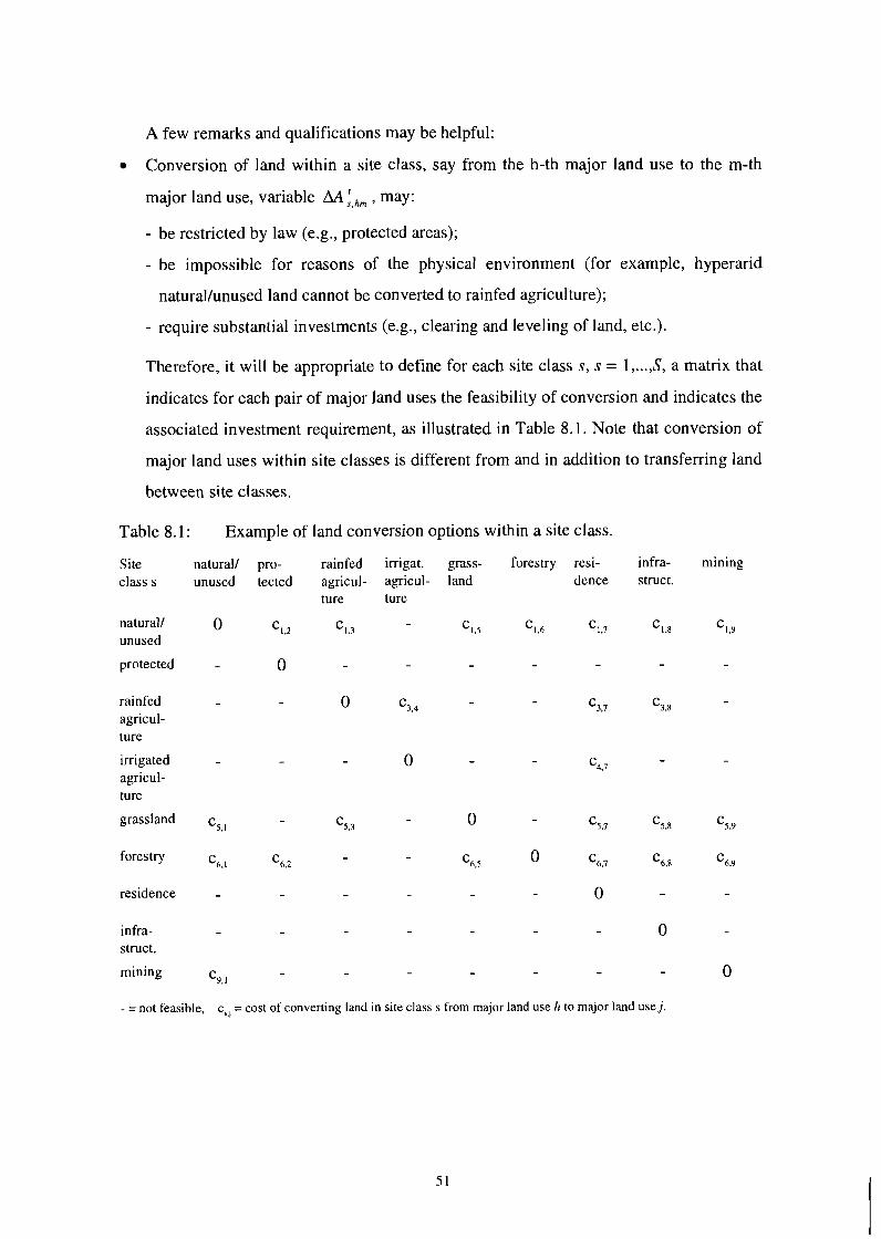
A few remarks and qualifications may be helpful:
Conversion of land within a site class, say from the h-th major land use to the m-th
major land use, variable AA .:,,, , may:
- be restricted by law (e.g., protected areas);
- be impossible for reasons of the physical environment (for example, hyperarid
natural/unused land cannot be converted to rainfed agriculture);
- require substantial investments (e.g., clearing and leveling of land, etc.).
Therefore, it will be appropriate to define for each site class s, s = 1, ..., S, a matrix that
indicates for each pair of major land uses the feasibility of conversion and indicates the
associated investment requirement, as illustrated in Table 8.1. Note that conversion of
major land uses within site classes is different from and in addition to transferring land
between site classes.
Table 8.1 : Example of land conversion options within a site class.
Site natural1 pro- rainfed irrigat. grass- forestry resi- infra- mining class s unused tected agricul- agricul- land dence struct.
ture ture
natural1 0 c1,2 c1,3 'l,5 %,7 c1.8 '1.9
unused
protected - 0 - - - -
- rainfed - - 0 - %,7 c3,8 c3.4 - agricul- ture
irrigated - - - 0 - C4,7 - - agricul- ture
grassland cSv1 - %,3 - 0 %,7 cs,8 5 . 9
forestry '6.1 '6.2 - - '6.5 0 '6.7 '6.8 C6,9
infra- - - - - - - 0 struct.
mining 1
- - - - - 0
- =not feasible, c,,, =cost of converting land in site class s from major land use h to major land use j.

Establishment of a land-use type k in site class s may involve intertemporal planning,
particularly in forestry. Therefore, we define three types of decision variables:
(i) activities denoting establishment of a land-use type k on a site class s in (current)
period t for harvesting in (a future) period z, AR:.:', ;
(ii) non-destructive harvesting activities, AH:.,, , where the main produce can be ob-
tained repeatedly without destroying the plant in the process of harvesting after
establishment of the land-use type. This applies, for example, to orchards, vine-
yards and various perennial plantation crops in agriculture;
(iii) destructive harvesting ('logging') activities, AL:.., , where by harvesting the pri-
mary produce, the land cover is removed so that it has to be followed by some re-
establishment activity before another harvest is possible; for instance, clear-cut-
ting of forest.
In the case of annual crops, establishment and harvest (destructive harvesting in our
terminology, since the plant is removed by harvesting) fall into one period, i.e.
AL:,, = AR:;', . Hence, the description can be simplified by including, by definition, the
establishment activities and costs with the harvesting activity.
Logging activities in forestry require proper establishment of land-use types, some-
times many periods in advance.
For annual crops, by definition, we observe:
ALf,,,, z = t AR;:; =
0, else '
for perennial crops and forestry we impose:
where At: denotes the minimum time required for establishing land-use type k in site
class s.
8.4 Land-balance conditions and constraints on land use
With these types of site class and land-use variables, as defined above, we proceed
with formulating land balance constraints that must be observed in the land allocation

procedure. First, we note that land allocated to different major uses in a site class s is
limited by the availability of that land qualityl7:
In general, there will be conversion of land between major land-use categories, de-
scribed by variables AAf.,, 2 0 . All land in a site class s must fall into one of the defined
major land-use categories:
There is a limit as to how much land can be transferred in any period between major
land usesl8:
It is further assumed that conversion of land between major use categories is limited to
land either newly entering the particular site class or having been subject to a destructive
harvesting ('logging') activity19 in the previous period:
Land available for establishment activities of various land-use types is limited by land
in a major land-use class, either available from previous destructive harvesting activities,
or resulting from net conversions between major land-use classes. In the specification of
these constraints, index sets I, denote the set of land-use types k that belong to major land-
use class h, e.g. wheat and potato cultivation are both land-use types belonging to crop
agriculture:
l7 Since we have defined a naturavunused major land-use class, we may assume an equality rather than an inequality to hold in (8.3).
1 8 ~ h e formulation of land conversion flexibility constraints shown here is just one possible specification. 19~eca l l that annual crops are always subject to 'logging'.

Land available for harvesting activities is limited to land previously established?
The treatment of land availability and land-use types, as introduced above, makes it
easy to extend the specification of constraints to also include livestock production. This is
particularly relevant with regard to ruminants. In that case two approaches can be
considered: (i) either the number of ruminant livestock units and estimated (generally site-
class specific) land requirements per livestock unit enter the respective land balance
equations above, or (ii) grasses (and other fodder crops) are defined as land-use types, and
the area and production of green-fodder is determined through a livestock feed-balance
constraint (e.g., see Fischer et al. 1994b). As outlined in Section 9, the latter approach is
more flexible and will be pursued in the LUC model.
In general, there will be limited resources other than land, e.g., irrigation water supply,
that are also essential to successful cultivation of various land-use types. In the LUC
model, we can distinguish two types of water supply that may exist in site class s, say
We.' and v.', denoting water supply available in fixed amounts and at a fixed cost (e.g.,
surface water), and variable water supply (e.g., pumped water described by a convex price-
dependent supply function), respectively. Let w , , . . denote water requirements of land-use
type k on site class s, and p,r the respective price of pumped water. Then we impose the
following set of constraints:
Note that constraint (8.9) could be used as a market-clearing condition to endogenize
variable water supply in the model, i.e., derive the price of pumped water from balancing
demand and supply.
'OHOW the allocation of extents in different major land-use classes to harvesting and logging activities of various land-use types can be modeled based on economic principles will be discussed in the next section.
In a similar way, labor input constraints in terms of family labor LF (fixed) and hired
labor LV (with a variable and price responsive supply) can be included, with I , , . , denoting
labor requirements of land-use type k on site class s.
Finally, environmental accounting and constraints can also be based on the concepts of
site classes and land-use types. For instance, let e, , ., denote emissions of type m per unit
of area of land-use type k, in site class s21. Given a maximum tolerable amount of emis-
sions of type m from site class s, the respective constraints would read:
In the model, these relationships (i.e., water supply, labor, and environmental
constraints) are reflected in the set of constraints that we have termed the transformation
function constraint in Section 6. Some of them apply to individual agents of the model;
others induce joint constraints for groups of agents. When decentralizing the welfare
program, the constraints will be implemented in the model through shadow price
mechanisms, or through 'trading' type of processes (like pollution permits), or through
rationing by a central institution (e.g., the government), depending on the characteristics of
each constraint.
8.5 Geographic representation of site classes
In the discussion on how to characterize and represent land resources and, land use, we
did not have to make any assumptions on what geographic representation, e.g., square
mesh of grid points or polygon-shaped map units, would be best suited for modeling. If the
grid size is not fixed ex-ante, as is often done in global change research (e.g., to 1" x I"
latitude - longitude grids), then any size polygons can be sufficiently well approximated by
adjusting the grid dimensions. Conversely, data on any grid size can be converted into
polygons. In the LUC model, we utilize pixel data in a gridded format. The advantage of
pixel-wise representation in a grid is twofold:
21 Emission coefficients can be time dependent. For convenience, we omit a time superscript.

- gridded data sets are easier and more practical to use in application programs;
- gridded data sets more readily allow the approximation of a continuous gradient of
geographic features (e.g., Keyzer 1992).
This second point is especially important. When working with gridded data, the
framework of site classes presented so far in this section remains valid, except that we
have to somewhat generalize the interpretation of site classes. Rather than being fixed (and
assumed homogenous) map units, site classes refer to a collection of grid points over
which certain attributes vary within a defined (narrow) range. Consequently, relationships
involving extents of site classes involve numerical integration, i.e., summation over a set
of grid points, say index set Is, of which a particular site class is comprised. For instance,
constraints in (8.11) could be written as:
(8.1 la)
However, there is also a cost to such increased accuracy and flexibility, when working
on a square mesh, since there will likely be a large increase in the number of decision
variables relating to the resource allocation problem.
9. Specification of supply and demand functions
Interactions between the supply of land-based commodities and their consumption is a
main driving force of land-cover change. In previous sections we have discussed this in
more general terms. In this section we set forth some model specifications and illustrate
the concepts with a few examples.
9.1 Production in the LUC model22
In economic models, production activities are usually organized in terms of economic
sectors. For instance in the LUC model, at the highest aggregation level, the following
sectors are distinguished: agriculture, forestry, and other non-agriculture. Sectors with a
strong relation to land use are further subdivided. In particular, this applies to agriculture
and forestry. The LUC sector representation is shown in Table 9.1.
In each sector a number of production conditions are distinguished. For example,
agricultural production in a compartment is described as cumulative output from a collec-
tion of representative farms23. Such differentiation should reflect major differences in
production conditions (agro-ecology, farm resources, infrastructure, etc.) and - for the
purpose of modeling land-use and land-cover change in the LUC project - relate to the
dominance of various driving forces. To be empirically founded, this requires appropriate
data sets and advanced methods of spatial statistical analysis, and builds on in-depth
analysis at representative case-study sites. Below we explain the approaches we use in
modeling the agriculture sector. These approaches are based on economic principles, are
consistent with the overall LUC modeling concept, allow the inclusion of technological
and structural information, and deal explicitly with yields, input use and land allocation.
2 2 ~ h i s section draws heavily on Keyzer (1982, 1987) and Folmer et al. (1995). 2 3 ~ o r economy of data collection and model building, the number of agents should be kept as small as pos-
sible, focused on the study objectives.

Table 9.1 : Economic sectors in the LUC model.
Product
wheat rice maize other
potato other
soybean other
sugar fruits vegetables
cotton other
sheep goats cattle buffalo other
pigs poultry&eggs other
fish
fish
logwood pulpwood fuelwood
logwood pulpwood fuelwood
power
power
Number
1
2
3
Sector
crops
livestock
fish
softwood
hardwood
energy
manufacturing
construction
transportation
other
Aggregate Sector
agriculture
forestry
other
Sub-sector
cereals
root & tubers
oilseeds
other food
-
non-food
ruminants
non-ruminants
marine
inland
biofuel
other
9.2 Modeling agricultural supply
There are several approaches to modeling agricultural supply. At least four different
types have been widely used:
(i) econometric models
(ii) linear programming (LP) models
(iii) simulation models of the systems dynamics type
(iv) revenue function approaches.
Traditional econometric models are inappropriate for the purposes of the LUC project
as they do not easily allow the inclusion of a priori technological information and struc-
tural relationships and constraints. In comparison, LP models follow an almost opposite
approach. The LP modeler specifies structural relationships, resource constraints, a priori
information on technology, etc., and assumes a rational 'farmer' who optimizes a measure
of economic efficiency, e.g., net revenue. The disadvantage of the LP approach is that the
resulting supply function is generally not a continuous function of input parameters, such
as prices and resource stocks, i.e., right-hand sides of the constraint matrix. This is unde-
sirable in the context of a welfare program because it complicates the solution procedure.
System dynamics simulation models are inconsistent with welfare analysis because they
are generally not based on accepted micro-economic principles. This class of models can
easily exhibit unacceptable properties and should be avoided in the normative approach.
The representation of agricultural supply in the LUC model is based on a combination
of nonlinear optimization and the revenue function approach, specifying the agricultural
supply model in a mixed primal-dual form derived from the general formulation (6.9) in
Section 6. It aims at maintaining the properties of the full primal mathematical program,
yet simplifies the solution procedures and parameter estimation by decomposing the
program (6.9) into several sub-problems. The sub-problems deal separately with, for in-
stance, input use and yield levels, acreage allocation to different cropping activities, live-
stock feed-mix, and livestock activity levels. These sub-problems are related by means of
feedback relationships that operate through linking constraints with known coefficient^^^.
This enables us to impose a priori information, like land balances or feed balance
constraints.
24As oposed to dual relationships that require parameter estimation.

The emphasis on decomposition is both for methodological considerations as well as
for reasons of efficient solution algorithms. Decomposition of (6.9) exploits the structure
of the full primal program to partition it into several sub-problems which are solved one
by one and, in general, are related to each other through feedback variables. Some obvious
advantages of such decomposition are:
- Each of the sub-problems is usually of a much smaller dimension than the full pro-
gram and may be solved more efficiently.
- Testing of specifications and parameter estimation greatly benefit from reducing the
dimensionality of the problem.
- Parameter estimation of resource allocation programming problems specified in pri-
mal form may be impossible due to lack of data on crop-specific input use (e.g., see
Folmer et al. 1995). For that reason (amongst others), economists have developed
dual approaches to facilitate model estimation.
- Solution algorithms can be tailored to exploit the specific features of individual sub-
problems.
Fortunately, the structure of an agricultural supply model may be conveniently
decomposed into several sub-problems. Let us start from the primal formulation of the
agricultural supply program. For a profit-maximizing producer, the supply program can be
written as in (6.9)25:
subject to:
Net production y' must be chosen from a feasible set Y' subject to: (i) constraints de-
fined by a transformation vector-function g(.) describing the available technology, (ii)
being consistent with available resource stocks kt, and (iii) the need to maintain stocks of
resources k"' for later time periods. In order to generate net outputs y' , producers allocate
2 5 ~ o r convenience of notation we drop the agent sub-script j.
resources k' to alternative production activities, each of which generates output of one26
commodity Qi , k = I , ..., K. A feasible allocation of resources @: = (@',,) of resources in
compartment c, at time t, is defined according to (9.927 (see also Section 7),
x @ ; s k', t = 1, ..., T
In Section 7 we defined the vector of resource stocks in a fairly broad sense, including
capital, machinery, labor, energy, input materials, land resources, water, etc. When
decomposing the full program (9.1), the aim is to partition the activity and resource
vectors @' and y' such that meaningful sub-problems can be solved separately. To exploit
specific features of the structure of agricultural supply, the general scheme of (9.1)
requires further specification. We model agriculture as consisting of two sub-sectors, i.e.,
crop cultivation and the livestock sub-sector. These are linked through competition for
some of the scarce resources in the region (e.g., labor, capital, water, land). The crop sub-
sector provides feedstuffs (green fodder as well as marketed feed concentrates) to the
livestock sub-sector. In addition, the livestock sector may provide fertilizer and draught
power to the crop sector. Therefore, with some additional assumptions about the structure
of the agricultural sector we can rewrite the profit function and constraint set of (9.1) as2?
subject to:
qk 'fkC(p,~k), ' I C
gc(A~, ' . * ,AK~) 'o
qk 2 hL(~,Vk)' k ' I L
gL(N,,...,NKL)s 0
where the vector functions f,(.) are yield response functions (see Section 9.3 below), q, is
yield, p, is the farm-gate price of output k, A, refers to area cultivated for activity k,
2 6 ~ i t h o u t loss of generality, we ignore the case of joint products which can be dealt with in the same way. 2 7 ~ o r the sake of simplicity we omit the compartment sub-script c.
2 8 ~ o simplify the presentation, let us now consider only one time period and drop, where not necessary for the understanding, the super-script indicating time.
belonging to the set of cropping activities, k E I,, and N, denotes livestock units for k
belonging to the set of livestock activities, k~ I,. V denotes the matrix of production
inputs V,, of type h into activity k, and jib is price of input type h. The vector functions
g,(.) and g, (.) are transformation constraints for the crop and livestock sub-sectors,
respectively. Vector function f (.) describes the constraints linking the two sub-sectors.
The specification of constraints in (9.4) decomposes the agriculture supply model into five
sub-problems: (i) determination of crop yields and inputs; (ii) land allocation in crop sub-
sector; (iii) determination of livestock yields and feed-mix; (iv) determination of livestock
numbers, i.e., allocation of operating capacity in livestock sub-sector; (v) allocation of re-
sources to crop and livestock sub-sector. The sub-problems are linked through feedback
relationships derived from optimality conditions. For instance, the shadow price of green-
fodder obtained by taking the derivative of the cost-function for the livestock sub-sector
with respect to feed requirement constraints must be consistent with the price used for
revenue calculation in the crop sub-sector model.
Clearly, decomposition and the solution procedure become more complicated when we
allow for possible transfers of resources between compartments or sub-sectors, as in
equation (7.6), and when intertemporal allocations are considered. Also, activities in the
forest sector may in some areas compete for common resources, such as land. Then, the
same type of decomposition technique is needed to deal with linkages between agriculture
and forestry.
9.3 Specifying yield relations
We turn now to one of the sub-problems of the agricultural supply model, the specifi-
cation of yield relationships and the determination of input use. In the LUC model, agro-
nomic information on crop yields are specified by a system of yield relations F,,(Vhk, V,) ,
k = 1 ,..., K, h = 1 ,..., H. Each of these relations indicates how much output Q, will be
obtained for a given combination of input V,, with a reference input V,, if other inputs are
not constraining. The reference input V,,, in our case land or animal units, is the input
which is common to all yield relations in the system. Since the system of yield relations
refers to the same output Q, and reference input V,,,
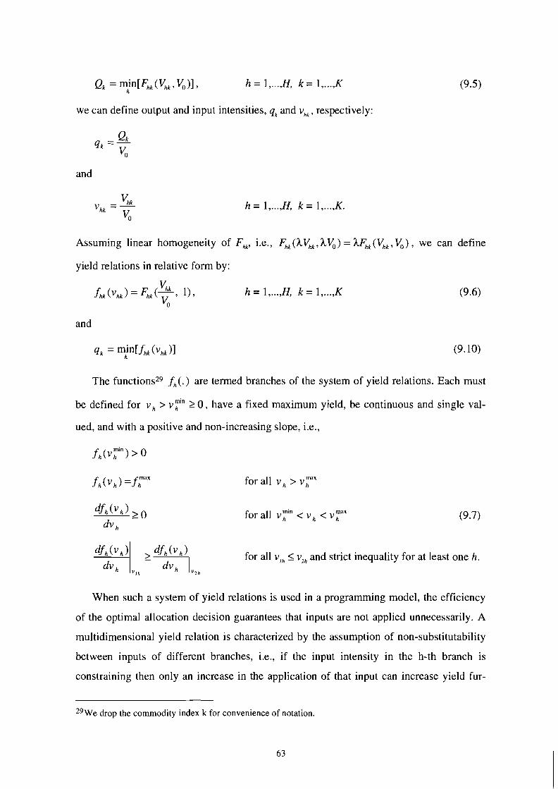
we can define output and input intensities, q, and v,, , respectively:
and
Assuming linear homogeneity of F,,, i.e., F,, (A&, ,A&) = hFhk (V,, , & ) , we can define
yield relations in relative form by:
v fhk(~hk) = F,k(+ 1)' h = 1 , ..., H, k = l , ..., K (9.6)
vo and
qk = min[fhk(vhk)l h
The functions29 f,,(.) are termed branches of the system of yield relations. Each must
be defined for v h > vYin 2 0 , have a fixed maximum yield, be continuous and single val-
ued, and with a positive and non-increasing slope, i.e.,
f h ( ~ , " " ) > 0
fh (vh) =fhmax for all v h > v,"""
for all v jf'" c v h c v r a x
dfh(vh) dfh (v h ) for all v,, I v,, and strict inequality for at least one h. dvh
When such a system of yield relations is used in a programming model, the efficiency
of the optimal allocation decision guarantees that inputs are not applied unnecessarily. A
multidimensional yield relation is characterized by the assumption of non-substitutability
between inputs of different branches, i.e., if the input intensity in the h-th branch is
constraining then only an increase in the application of that input can increase yield fur-
2 9 ~ e drop the commodity index k for convenience of notation.
63

ther. For the broad categories of inputs to be represented in the LUC model (e.g., solar ra-
diation, water, energy, fertilizer), this seems warranted. For instance, it is acceptable to as-
sume that fertilizers cannot be substituted for water, nor can nitrogen fertilizer be substi-
tuted for phosphates. One can then model agricultural supply, for example, by net revenue
maximization. For a set of crops k = 1 ,..., K, given output prices p, and input prices p, , and
levels of reference input V,, > 0 (here the common input A,=V,,, denotes acreage allocated
to crop k), we can write:
subject to:
We define the cost function c,(q,) of producing crop k with yield intensity q,:
where v,,(q,) is the inverse function of f,,(v,,), indicating how much input of type h is re-
quired to obtain a given yield g,. Revenue maximization can then be obtained by solving
for an optimal solution q* so as to equate marginal costs with marginal revenue:
With some additional complication of mathematical notation and algebra, the system
of yield relations can also be formulated to handle aspects such as joint products,
constraints on inputs, substitution between human and machine labor, and livestock
production (e.g., see Keyzer 1982).
9.4 Consumer demand
Recall from the previous sections that we distinguish a number of commodities, in-
dexed k = 1, ..., K. A list of commodities to be considered at the retail level is shown in
Table 9.2. The consumption of consumer i in time period, t = 1, ..., T, is described by a
consumption vector xIf = (xI!, , . . . , X& ) . The consumer is limited by a budget constraint.
Suppose the market price of commodity k at time t is p: and p' = (p: ,...,pi) is a vector

of commodity prices. Income hi' of consumer i at time t is generated from exchange of
endowments w,! (i.e., resources, sales of stocks, wage labor) and transfer payments b: :
hi' = ( P ' , w , ! ) + ( p ' , ~ . O b y ~ ) + b ~ , I (9.10)
where 0; is the share of consumer i in firm j at time t. (For the sake of simplicity of nota-
tion we do not consider taxation policies here). Therefore, the cost of the respective con-
sumption bundle x,' is (p ' ,~ ,~)=C~p;x , ! , , and the budget constraint at time t reads
(pt,x,!) 5 h;.
Table 9.2: Example of retail commodities in the LUC model.
Number
1
2
3
Sector
agriculture
forestry
other
Sub-sector
cereals
roots and tubers
oils and fats
other food
non-food
meat
milk
fish
wood products
energy
manufacturing
construction
transportation
other
Commodity
wheat rice other grains
roots
vegetable oil animal fat
sugar fruits vegetables
cotton other bovine and ovine pork, poultry, eggs dairy products
fishery products
logwood pulpwood fuel wood
fuel electricity
#
1 2 3
4
5 6
7 8 9
10 11 12 13
14
15
16 17 18
19 20
2 1
22
23
24

Any vector x,! 2 0 satisfying the budget constraint is regarded as a feasible demand of
consumer i. Note that the feasibility of a demand trajectory xi = (xI0 ,..., xiT) depends on
prices p = (pO ,... , pT) and income hl = (ho ,..., h') . Any vector function xi(p, hi) satisfying
the budget constraints for given p and h, can be considered a demand system. Demand
systems are typically obtained through econometric estimation. Various specifications
have been derived from utility maximization, based on flexible specifications of the utility
function. Assume the preferences of consumer i are described by an intertemporal utility
function y(xi). Then, the vector function xi(p,hi) comprising the optimal solutions obtained
by maximizing utility ui(xi) subject to budget hi represents a demand system.
Various specifications befitting econometric estimation of parameters have been
proposed in the literature. A well-known (and particularly simple) example is the demand
system derived from a log-linear specification of the utility function, the Stone-Geary util-
ity function, that has been often used in applied modeling. It is of the following form
(dropping for convenience the subscript for consumer i):
which results in an explicit representation of the demand system x(p,hi) as:
When a large number of commodities is considered, as in the LUC model, nesting of
the commodity tree is a standard technique for obtaining more robust estimates. For
instance, Michalek and Keyzer (1992) discuss a two-stage approach applied to modeling
(per capita) consumer behavior in the member countries of the EU, where at the higher
level aggregate demand was estimated using an Almost Ideal Demand System, and for
each commodity group separately (yet consistently) a Linear Expenditure System like in
(9.12) was specified.
10. Risks and uncertainty
Up to now, we have assumed that the agents in the model have perfect foresight and
act under full certainty. Of course, in reality, consumers, producers and governments do
not have access to all the information they need to maximize intertemporal utility and
profit. They are faced with uncertainty about their external environment (prices, markets,
weather) and about their own production set (productivity of workers, reliability of equip-
ment). Insurance schemes, a common mechanism to cope with and share risks, cannot be
introduced for all possible uncertainties and risks involved. In practice, the aim is to
combine economic schemes (like insurances), where they are feasible, with the choice of
policies that are robust against possible 'surprises'.
Uncertainty can be incorporated into optimization models, although this often leads to
formulations which are intractable for applied work unless specialized tools are developed.
However, disregarding uncertainty completely may lead to extreme supply reactions and
over-specialization. For example, unrealistic combinations of crops entering the optimal
solution is a common problem in deterministic optimization problems. It is often the case
that the optimal solution in some compartment is dominated by crop specialization if
uncertainty is ignored. In practice, risks associated with weather and the effects of other
'exogenous' and sometimes transient variables lead to diversification in crop mixes.
The land-use change study has to deal with at least two quite different types of uncer-
tainties: (i) Objective uncertainty, say about rainfall in a particular year. A model builder
shares this type of uncertainties with the agents (farmers, etc.) in the real world; (ii) Uncer-
tainties of the model builder with respect to the quantification and specification of rela-
tionships, to the value of certain technical parameters, or to the political feasibility of im-
plementing intended policies.
10.1 Sources of uncertainty
Uncertainty (and hence risk) exists due to a variety of reasons. We list examples of
some important real-world sources of risk:
Variability of climate is a major concern of farmers in many parts of the world. In arid
and semi-arid regions, rainfed agriculture is particularly sensitive to drought risks, and to
variability in amount and distribution of rainfall. In other areas, notably fertile and densely

populated flood plains, the risk of flooding and water logging influences land-use
strategies. Other risks, e.g., typhoons, hailstorms and frost, threaten human lives and crops
with varying intensity. Global warming may increase the risk of the occurrence of extreme
events.
Biological processes involved in agricultural production are also subject to
environmental variations which can be difficult to control and give rise to unstable
supplies. For instance, agriculturists in less developed regions face the risk of damage
from pests and diseases that may be beyond their means of control.
The institutional and political setting within which decisions on land use take place
may be uncertain as well. The future orientation of the Common Agricultural Policy
(CAP) in the European Union may be as uncertain to many EU farmers as is the success of
economic transformation and privatization in Eastern Europe and the former Soviet Union.
There may also be uncertainties as to future environmental standards and limitations on
land use. For example, the scientific uncertainty about the impacts of greenhouse gas
emissions and potential global warming also affects planning and development in agricul-
ture and forestry. A consequence of industrialization and increased use of fossil fuels is
often acidification of soils which may hamper their buffering capacity and magnify the
risk of 'chemical time-bombs, i.e., the rapid release of toxic substances from soils to the
surrounding environment, in particular to groundwater.
There is also uncertainty about longer-term technological progress. What kind of tech-
nologies will be available to produce food, fibers and timber, or to cope with environ-
mental problems and clean-up? At what cost will such technologies be available?
Furthermore, there are various uncertainties that relate to behavioral aspects of socie-
ties and economic agents. For instance, the dynamics of value systems and hence the
preference structure of consumers cannot be known with certainty. Also, economic agents
as well as governments may not be willing to reveal information to each other. Therefore,
the future prospects of markets may be difficult to judge, resulting in major uncertainties
as to future costs and benefits of investments. Investment decisions may involve irreversible
transformations of the environment, or at least may be characterized as extremely costly in
terms of options to reverse their impacts, but such consequences are difficult to predict.

Finally, there are methodological uncertainties. Non-stationarity and dynamics of dise-
quilibrium have often been quoted as driving forces of economic processes. The existence
of a unique equilibrium solution has been proven only under fairly strong assumptions
about functional relationships describing demand and supply of commodities. When mul-
tiple equilibrium solutions exist there is uncertainty as to what processes lead to the selec-
tion of particular solutions and what the sensitivity is of this solution with regard to initial
conditions.
We have listed a range of uncertainties that limit our ability, in fact render it impossi-
ble, to predict the future path of the interacting socio-economic and environmental
systems. Some of the uncertainties can be included formally in the specification of the
model components, i.e., the description of particular agents. Others are dealt with in a
more general way by means of scenario assumptions and a policy framework. Rather than
computing one solution for every possible outcome, which would lead to insurmountable
problems of screening results, the study follows a stochastic programming approach,
incorporating major uncertainties and appropriate economic mechanisms within the
stochastic optimization model itself (Ermoliev and Fischer 1993).
10.2 Variability in farm production conditions
Traditional models often ignore possible variability in production conditions, simply
by averaging them. This is equivalent to dealing with only one scenario of possible de-
velopments. In general, however, there may be an infinite number of scenarios, and the
challenge is to find policies robust against all or most eventualities. Averaging deprives us
of the diversity which may be necessary to meet risks, and may lead to wrong conclusions.
Let us illustrate this by the following examples:
Examule 10.1: Suppose there are two farms with the same crop structure and average
yields, but with different variability of yield, e.g., due to weather conditions. It is clear that
the farm with a larger variance in yields is more vulnerable and may be less profitable, but
it is impossible to distinguish them on the basis of averaged data.
Example 10.2: Suppose there is only one type of soil and two crops, A and B. Crop A per-
forms better in dry seasons, and crop B outperforms crop A in wet seasons. On average,
the weather condition may only be dry or wet, implying a mono-cropping structure as an

optimal solution, i.e. cultivation of only crop A or only crop B. By taking into account
probabilities for both weather conditions, dry and wet, the structure of the optimal solution
is changed to a multicropping structure. Crop A and crop B are both included in the
optimal solution in proportions related to frequencies of wet and dry seasons, prices on the
market, etc.
10.3 Two-stage decision processes
In the short term, the sustainable supporting capacity of a region, limited by prevailing
conditions in 'bad' years, depends on the region's ability to adapt to changing conditions,
e.g., through additional land management measures, food storage, or finance of additional
imports and infrastructure for distribution. In the longer term, strategic decisions are
needed to keep pace with the changing needs in a region. In the LUC model, these aspects
are taken care of by incorporating two types of mechanisms:
Long-term (ex-ante) strategic decisions such as investment in machinery, irrigation
schemes, storage facilities, major land improvements, structure of livestock and
cropping patterns, and
Short-term adaptive (ex-post) decisions such as use of irrigation water, level of fer-
tilizer application, allocation of manual labor and machinery in a given situation,
change of planting dates, replanting of crops, etc.
Yields of crops and livestock are a result of human activity and management skills
involving both ex-ante and ex-post decisions, and of natural endowments and characteris-
tics, some of which are uncertain, like the occurrence of extreme events such as floods,
droughts, or accidents.
Assume that each of these uncertain factors can be characterized by a finite number of
scenarios with weights describing associated frequency distributions. For example,
weather conditions could be classified by three30 situations (scenarios): (1) dry season with
frequency F,, (2) wet season with frequency F,, and (3) 'normal' season with frequency F,.
Other uncertain elements, such as technological innovations, could also be represented by
a number of scenarios with subjective probabilities. Therefore, generally speaking, each
' O 0 f course, more details could be incorporated, like characterizing weather conditions as 'dry and cold', 'dry and hot', 'wet and cold', etc.

scenario can be described by a vector s of integer numbers, s = (s,, ..., s,), where the com-
ponents s,, ..., s, are random variables assuming a finite number of integer values with
given frequencies (probabilities). For example, S,E Is,,, s,,, ...) may represent scenarios of
weather, s , ~ IS,,, s,,, ...I describes scenarios of flood hazard, s , ~ IS,,, sj2, ... ) models
scenarios of possible technological innovations, etc. Note that although the number of
possible situations (scenarios) is finite, it may easily become very large.
Another important question relates to the dynamic aspects of the system and the timing
of decisions. The ex-ante decision variables can be thought of as trajectories of strategic
decisions over periods t = I , ..., T. The notion of ex-ante time dependent decisions is related
to each particular period t and scenario s.
A scenario s then is itself comprised of a trajectory, s = (s(I), ..., s(T)), where the
components s(I), ..., s(T) are random vectors. For instance, each s(t) may assume values
s,,s, ,..., s, with probabilities F,,F ,,..., F, (which may themselves depend on time). Such
types of models, even when the number of possible situations S for a given time period t is
small, may require special stochastic optimization techniques, as the number of all
possible combinations for t = 1, ..., T may become astronomical. Hence, it may prove
impossible or impractical to list and evaluate all possible combinations of situations, as
would be required to solve the optimal decision problem by conventional optimization
tools.
10.3 Irreversible decisions
There is yet another issue of risk and uncertainty to be discussed. Strategic (ex-ante)
decisions are defined as those which cannot be altered in response to an observed situation.
In order to ensure flexibility of a system under such decisions, they are supplemented by a
set of corrective (ex-post) decisions. Some strategic decisions, for instance, such as placing
a dam, the use of nuclear energy, deforestation of tropical rainforests, etc., may involve
irreversible transformations of the environment, or at least may be characterized as ex-
tremely costly in terms of options to reverse their impact. There is often considerable un-
certainty at the time when a decision must be taken, as to future costs and benefits associ-
ated with the irreversible decision.

In order to reduce the risks involved in irreversible decisions, Arrow and Fisher (1974)
suggested that, in the presence of uncertainty, decisions should be only partially accepted
and applied in the initial stage, and can then be corrected by learning from experience. For
example, under-investment can be remedied before the second time-period; uneconomic
over-investments, although impossible to be corrected, would be limited so as to avoid
costly losses. The challenge is to determine the robust elements of irreversible decisions
for adoption during the initial stage.
We consider now a simple example illustrating that an otherwise appropriate
formulation of a supply model may be inadequate and degenerate to simplistic conclusions
without consideration of an (at least) two-stage decision process. For example, the
productivity of land at a given geographical location is an indicator of the local economic
conditions and environmental properties. These are subject to stochastic variation as well
as dynamic changes. Land productivity may be affected, for instance, by variations in
water supply which may be due to seasonal or inter-annual fluctuations, i.e., stochastic, or
to a changing climate, i.e., a dynamic change manifesting itself in a gradual change of
stochastic properties, e.g. frequency of droughts or floods. The example demonstrates that
the value of land in a particular region is a rather complicated function of different factors.
An analysis of the sensitivity of this function to potential climate change, through
variations of water resources, may reveal that their relevance to the welfare of the region is
negligible as compared to, for instance, mismanagement of regional capital resources or
accidental pollution (Ermoliev and Fischer 1993).
Consider a region with only two compartments. The agricultural performance of the
first compartment can be improved by irrigation, whereas in the second compartment addi-
tional water resources are not available. Furthermore, the maximum level and efficiency of
irrigation depends on the water level of the river. If the water level is characterized by its
average amount, the decision to use irrigation is trivial and depends, for instance, on
whether the net revenue per hectare of irrigated area in the first compartment is greater
than the profit from a hectare without use of irrigation. The stochastic variation of the river
water level creates essential differences. In situations of low water levels, the land pre-
pared in advance can only be partially supplemented with additional water. Besides these
physical limitations, profits will also be affected by variations in water price. It is possible

that in a dry season the use of irrigation water may become unprofitable although
irrigation is beneficial at average conditions.

11. Summary
The LUC project is aimed at the analysis of spatial and intertemporal interactions
among various socio-economic and biogeophysical factors that drive land-use and land-
cover change. Exact prediction of such complex systems over medium and long time-
horizons is impossible. Instead, we emphasize the role of comparative studies of the
impacts from various demographic, economic and political factors on the dynamics of
land-use and land-cover change. Taking this into account, a model specification where
policies and decisions of economic agents are explicitly introduced becomes essential.
From an economic perspective, the interactions between climate, land resources and
vegetation are part of physical transformation processes of resource and capital stocks in-
duced by human investments and dis-investments. A key interest is in describing patterns
and conditions of land resources development and investment that are Pareto-efficient, i.e.,
such that no one could be better off without someone else being worse off. In this analysis,
equity considerations are obviously relevant as well. Otherwise, these investments may
leave certain regions without sufficient resources or deprive future generations.
In the LUC project, the intention is to describe such socially desirable and
economically efficient trajectories of investments and resource use. These trajectories
represent a welfare optimum in which the levels of investments are determined and with
weights on the individual agents' utilities set so as to have them satisfy their budgetary
(and other) constraints. Though such a solution may be regarded an unachievable ideal, it
can serve to draw a line between real-world problems (i) that are due to fundamental
technical relations, or to incompatible dynamics, e.g., of population growth, and (ii) those
which are attributable to specific modes of social organization and institutional setting.
While the former will persist in any projected trajectories of future development, the latter
only appear as one introduces imperfections in the decentralization of the welfare opti-
mum. After the specification of technical relations, and the characterization and computa-
tion of a welfare optimum, the issue of decentralization can be addressed. Here, the focus
lies on external effects in production, i.e., effects on resource accumulation that are not
conveyed through commodity prices, in which case corrective policy actions may be re-
quired.
The task poses some essential methodological challenges of this task. The study of
spatial and intertemporal interactions and the computation of consistent welfare weights
leads to large-scale nonlinear problems where uncertainty and unpredictability play an
essential role in the overall evaluation of different policies.
External effects are present in virtually all environmental problems, because at present,
resources, like fresh air and clean water, are often not being priced appropriately, i.e.,
valuations do not take into account all the services that are directly or indirectly provided
to society. Hence, excessive utilization by some will always have external effects on
others. The LUC project aims to make this notion more precise in several respects. For
example, simulations with the LUC model may illustrate that due to its beneficial effect on
climate, any land with an intact vegetation cover produces valuable 'output', even if no
human activity is undertaken on it.
Once an adequate mode of decentralization has been found, an attempt will be made to
incorporate the real-world imperfections that explain the difference between observed
trends and welfare-optimal trajectories. This part of the analysis may have to be crude, due
to paucity of data and also due to the necessary level of aggregation in the continental-
scale LUC model. Yet, this final part of the analysis should go beyond the formulation of
'ideal' policies and suggest policies that are both realistic and conducive to reaching long-
term sustainability.
To achieve the objectives outlined in this paper, the activities of the LUC project in the
continental-scale study are organized at three broad levels, as shown in Figure 11.1. The
most general stratum is termed the scenario framework. Data collection and analysis at
this level serve (i) to embed the study region in the wider geographical global context, and
(ii) to develop trajectories of variables which are not dealt with inside the LUC model, but
that are important to the decisions of consumers, such as income derived from non-land-
based economic sectors (i.e., other than agriculture and forestry), and to the decisions of
land-managers, including policy-formulation, technological development, and possible
changes of the climate system (Toth 1995).
The second stratum of the organization refers to the continental-scale study region. At
this level, a geographic information system and databases, the LUC-GIs, is being
developed that will allow for various biogeophysical assessments in relation to the
dynamics of natural vegetation (van Minnen et al. 1995), land productivity (Rosenzweig et
al. 1995), land degradation, and hydrology, and for the analysis of socio-demographic
factors (Heilig 1995). These analyses are essential inputs to the database and
parameterization of the centerpiece of the LUC study, the LUC Core Model, which has
been outlined in this paper.
In parallel to and in support of the development of the continental-scale LUC model,
several case studies in representative ecological and socio-economic settings are being un-
dertaken. These case studies are implemented by local study teams and provide the oppor-
tunity for in-depth analysis of regionally specific land-use issues. A number of case study
areas have been identified and collaborating teams established in China, Japan and Russia.
Figure 1 1.2 shows the geographical distribution of the case study sites within the continen-
tal-scale study region.

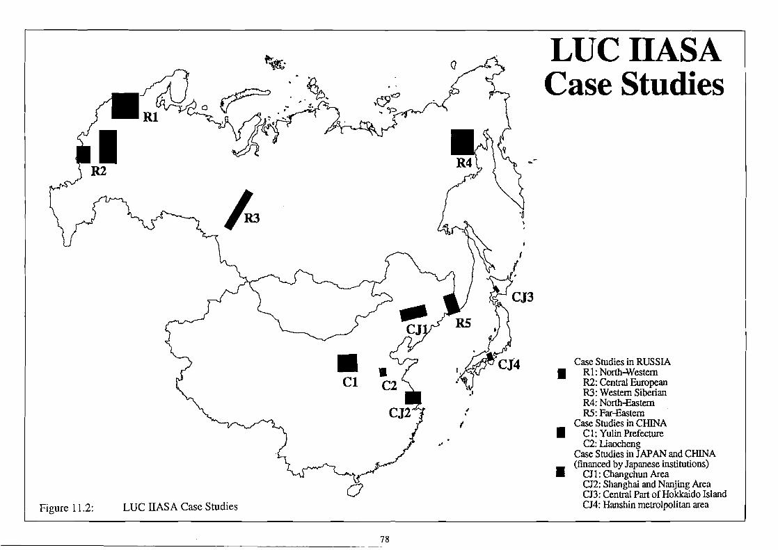
LUC IIASA Case Studies
Case Studies in RUSSIA a R1: Northqestem R2: Central European R3: Western Siberian R4: NorthEastem R5: Far-Eastern
Case Studies in CHINA 1 Cl: Yulin Prefecture
C2: Liaocheng Case Studies in JAPAN and CHINA (financed by Japanese institutions)
1 CJ1: Changchun Area CJ2: Shanghai and Nanjing Area CJ3: Central Part of Hokkaido Island CJ4: H'ulshin metrolpolitan area

References
Adams, D.M., R. Alig, J.M. Callaway, B.A. McCarl, 1994. Forest and Agriculture Sector Optimizaion Model: Model Description. RCGMagler Bailly, PO Drawer 0 , Boul- der, CO 80306-1906.
Adams, R.M., R.A. Fleming, C. Chang, B.A. McCarl, and C. Rosenzweig, 1993. A Reas- sessment of the Economic Effects of Global Climate Change on U.S. Agriculture. Oregon State University.
Alcamo, J. (ed.), 1994. IMAGE 2.0: Integrated Modeling of Global Climate Change. Klu- wer Academic Publishers, Dordrecht.Binswanger, H. P. and V. W. Ruttan, 1978. Induced innovation: Technology, institutions and development, Johns Hopkins University Press, Baltimore.
Armington, P.A., 1969. A theory of demand for products distinguished by place of pro- duction. IMF Staff Papers, (1 6): 159-178.
Arrow, K. J. and A. C. Fisher, 1974. Environmental Preservation, Uncertainty and Irre- versibility. The Quarterly Journal of Economics, 2, 3 12-3 19, 1974.
Brinkman, R., 1987. Agro-ecological characterization, classification and mapping. Dif- ferent approaches by the international agricultural research centres. In: A.H. Bunting (eds.), Agricultural Environments. Characterization, Classification and Mapping. C.A.B. International, Wallingford, UK, pp. 3 1-42.
Brooke, A., D. Kendrick and A. Meeraus, 1992. GAMS, a User's Guide, Release 2.25. Dan- vers, MA: International Thomson Publishing.
Burmeister, E., 1980. Capital theory and dynamics. Cambridge University Press, Cam- bridge.
Debreu, G., 1959. Theory of value. Wiley, New York.
Emanuel, W.R., Shugart, H.H. and Stevenson, M.P., 1985. Climatic change and the broad-scale distribution of terrestrial ecosystems complexes. Climatic change, 7: 29-43.
Ermoliev, Y. M. and G. Fischer, 1993. Spatial modeling of resource allocation and agri- culture production under environmental risk and uncertainty. WP-93-11, Interna- tional Institute for Applied Systems Analysis, Laxenburg, Austria, 38 pp.
FAO, 1978. Report on the agro-ecological zones project. Vol 3. Methodology and results for South and Central America. World Soil Resources Report 4813. , Food and Ag- ricultural Organization of the United Nations, Rome, pp. 25 1.
FAO, 1995. World Agriculture: Towards 2010, An FA0 Study. Edited by N. Alexandratos, Food and Agricultural Organization of the United Nations and J. Wiley & Sons, England, pp. 488.
FAOIIIAS A, 1993. Agro-ecological assessments for national planning: the example of Kenya. FA0 Soils Bulletin 67, FAO, Rome.
FAOIIIASAAJNFPA, 1982. Potential population supporting capacities of lands in the de- veloping world. Technical Report on Project INTI5 13, FAO, Rome.
Fischer G., K. Frohberg, M.A. Keyzer, and K.S. Parikh, 1988. Linked national models: A tool for international policy analysis. Kluwer Academic Publishers, Netherlands,
214 pp.
Fischer, G., Y. Ermoliev, M.A. Keyzer, 1993. Towards integrated modeling of land-use and land-cover change under environmental risk and uncertainty. Paper prepared for Oxford Workshop on Land-Uselcover Change (IGBP-HDP), Oxford 16-19 November, 27 pp.
Fischer, G., K. Frohberg, M. L. Parry, and C. Rosenzweig, 1994a. Climate change and world food supply, demand and trade: Who benefits, who loses?, Global Environ- mental Change 1994 4(1):7-23.
Fischer, G. and J. Antoine, 1994b. Agro-ecological land resources assessment for agricul- tural development planning, A case study of Kenya, Making land use choices for district planning. World Soil Resources Report 7119, Food and Agriculture Or- ganization, Rome, and International Institute for Applied Systems Analysis, Lax- enburg, Austria, 84 pp.
Fischer, G. and H.T. van Velthuizen, 1995. Climate change and global agricultural po- tential, A case study of Kenya. WP-95-??, International Institute for Applied Sys- tems Analysis, Laxenburg, Austria, (forthcoming), 50 pp.
Folmer, C., M.A. Keyzer, M.D. Merbis, H.J.J Stolwijk, and P.J.J Veenendaal, 1995. The Common Agricultural Policy beyond the MacSharry Reform. Elsevier Science, North-Holland, Amsterdam.
Forrester, J.W., 197 1. World Dynamics. Wright Allen Press.
Ginsburgh, V. and M.A. Keyzer, (forthcoming). The structure of Applied General Equi- librium Models. Cambridge, Mass.: MIT-Press.
Guang, X. and W. Zhihong, 1993. Climate change and its technical and institutional ad- aptations: China's perspective. Workshop on Mitigation, Impacts and Adaptation to Climate Change, International Institute for Applied Systems Analysis, Laxen- burg, Austria.
Gunning, J.W. and M.A. Keyzer, 1995. Applied general equilibrium models for policy analysis, in: J. Behrman and T.N. Srinivasan (eds.), Handbook of Development Economics, Vol. IIIA, Amsterdam: North Holland.
Hayami, Y. and V. W. Ruttan, 1985. Agricultural development: An international perspec- tive. Johns Hopkins University Press, Baltimore.
Heilig, G., 1995. Anthropogenic Driving Forces of land-use Change in China. Working Paper, International Institute for Applied Sytsems Analysis, Laxenburg, Austria, 4 1 ~ ~ .
Hertel, T.W. (ed.), 1995. Global trade analysis: Modeling and applications. Cambridge University Press, (forthcoming).
Houghton, R.A., 199 1. Releases of carbon to the atmosphere from degradation of forests in Tropical Asia. Canadian Journal of Forestry Research, 21 : 132-142.
Hulme, M., Wigley, T., Jiang, T., Zhao, Z.-c., Wang, F., Ding, Y., Leemans, R. and Mark- ham, A., 1992. Climate change due to the greenhouse efSect and its implications for China. WWF, Gland, Switzerland, 57 pp.
Jin Z., D. Ge, H. Chen, and J. Fang, 1995. EfSects of Climate Change on Rice Production and Strategies for Adaptation in Southern China. In: Climate Change and Agriculture: Analysis of Potential International Impacts, edited by C. Rosenzweig,

J.T. Ritchie, J.W. Jones, G.Y. Tsuji, and P. Hildebrand, ASA Special Publication Number 59.
Keyzer, M.A., 1982. On the representation of technical information in an agricultural programming model. Staff working paper SOW-82-5, Centre for World Food Studies SOW-VU, Free University, Amsterdam.
Keyzer, M.A., 1987. On the specification and parameter estimation of a decomposed, mixed primal-dual model of agricultural supply. Staff working paper SOW-87-15, Centre for World Food Studies SOW-VU, Free University, Amsterdam.
Keyzer, M.A., 1992. Land evaluation: Towards a model representation. Staff working pa- per SOW-92-05, Centre for World Food Studies SOW-VU, Free University, Am- sterdam.
Keyzer, M.A., 1994. Resource conservation in overlapping generation models. Invited paper at the EAAE-Seminar held in Vienna on The role of agricultural externalities in high income countries. Staff working paper SOW-94-06, Centre for World Food Studies, Amsterdam.
Kitamura, T., M.L. Parry, G. Fischer, R. Leemans, V. Rojkov, Y. Satoh, V. Stolbovoy, F. Toth, and Y. Liu, 1994. Modeling land use/cover change in Europe and Northern Asia. A proposal to the International Institute for Applied Systems Analysis, Inter- national Institute for Applied Systems Analysis, Laxenburg, Austria, (unpub- lished).
Leemans, R. and Solomon, A.M., 1993. The potential response and redistribution of crops under a doubled C02 climate. Climate Research, 3: 79-96.
Malthus, T.R., 1982. An Essay on the Principle of Population, as it effects the future im- provement of society (1798). Hammondsworth: Penguin Classics.
Meadows, D.H., D.L. Meadows, J. Randers and W.W. Behrens, 1972. The Limits to Growth: A report for the Club of Rome's project on the predicament of mankind. London: Earth Island.
Norse, D., 1993. Towards a design for a LUCC modelling system. Briefing Paper prepared for the Oxford Workshop on Land-Uselcover Change (IGBP-HDP), Oxford 16- 19 November, 7 pp.
Parry, NI.L., Carter, T.R. and Konijn, N.T. (eds.), 1988a. The Impact of Climatic Varia- tions on Agriculture. Volume 1: Assessments in Cool Temperate and Cold Re- gions. Kluwer Academic Publishers, Dordrecht. 876 pp.
Parry, M.L., Carter, T.R. and Konijn, N.T. (eds.), 1988b. The Impact of Climatic Varia- tions on Agriculture. Volume 2: Assessments in Semi-arid Regions. Kluwer Aca- demic Publishers, Dordrecht. 764 pp.
Parton, W. J., D. S. Schimel, C. V. Cole and D. S. Ojima, 1987. Analysis offactors con- trolling soil organic matter levels in Great Plains grasslands. Soil Sci. Soc. Am. J. 51:1173-1179.
Parton, W. J., J. W. B. Stewart, and C. V. Cole, 1988. Dynamics of C, N, P and S in grassland soils: a model. Biogeochemistry 5: 109- 13 1.
Parton, W. J., J. M. 0 . Scurlock, D. S. Ojima, T. G. Gilmanov, R. J. Scholes, D. S. Schimel, T. Kirchner, J.-C. Menaut, T. Seastedt, E. G. Moya, A. Kamnalrut, and J. I. Kinymario, 1993. Observations and modeling of biomass and soil organic mat-

ter dynamics for the grassland biome worldwide. Global Biogeochemical Cycles, 7:785-809.
Rosenberg, N. J., and P. R. Crosson, 1991. The MINK project: A new methodology for identifying influences oJ and responses to, increasing atmospheric carbon dioxide and climate change. Environmental Conservation, 18:3 13-322.
Rosenzweig, C., M.L. Parry, G. Fischer, and K. Frohberg, 1993. Climate change and world food supply. Research Report No. 3., Environmental Change Unit, Univer- sity of Oxford, Oxford, 28 pp.
Rosenzweig, C. and A. Iglesias, 1995. Modeling land-use and land-cover changes in Russia and Northern China. Research protocol for agricultural assessment. Working Paper, International Institute for Applied Systems Analysis, Laxenburg, Austria.
Ruttan, V. W. and Y. Hayami, 1988. Induced technical change in agriculture. in: Agricul- tural productivity measurement and explanation, S. M. Capalbo and J. M. Antle (eds.), Resources for the Future, Washington D.C.
Simpson, J. R., 1993. Urbanization, agro-ecological zones and food production sustain- ability. Outlook on Agriculture 22(4):233-239.
Solomon, A.M., 1986. Transient responses of forests to C02-induced climate change: simulation modeling in eastern North America. Oecologia (Berlin), 68: 567-579.
Stem, P. C., 0 . R. Young, and D. Druckman (eds.), 1992. Global environmental change: understanding the human dimensions. National Research Council Report, Wash- ington D. C.
Tiffen, M. and M. Mortimore, 1992. Environment, population growth and productivity in Kenya: A case study of Machakos district. Development Policy Review, vol. 10, pp. 359-387.
Toth, F., 1995. The socio-economic context of land-use changes in Europe and Northern Asia. Working Paper, International Institute for Applied Systems Analysis, Laxenburg, Austria.
Turner, B.L., 11, Clark, W.C., Kates, R.W., Richards, J.F., Mathews, J.T. and Meyer, W.B. (eds.), 1990. The Earth as transformed by Human Action: Global and Regional Changes in the Biosphere over the past 300 years. Cambridge university Press, Cambridge. 725 pp.
Turner, B.L., 11, Moss, R.H. and Skole, D.L., 1993. Relating Land Use and Global Land- Cover Change: A Proposal for an IGBP-HDP Core Project. IGBP Rep. No. 24 and HDP Rep. No. 5., International Geosphere-Biosphere Programme and the Hu- man Dimensions of Global Environmental Change Programme, Stockholm, pp. 65.
UNEP/ISSS/ISFUC/FAO, 1995. Global and national soils and terrain digital databases (SOTER), Procedures manual (revised edition). V.W.P. van Engelen and T.T. Wen (eds.), International Soil Reference and Information Centre, Wageningen, The Netherlands, 1 25 pp.
van Minnen, J.G., G. Fischer, and V. Stolbovoi, 1995. A Land-Cover Classification for Modeling Natural Land Cover within the IIASA LUC Project, Working Paper, International Institute for Applied Systems Analysis, Laxenburg, Austria.
van Velthuizen, H.T., G. Fischer, M.M. Saleem, M.M. Shah, and R. von Kaufmann, 1995. Potential of forage legumes in land-use intensification. Towards sustainable crop-

livestock systems in West Africa. Vol. 1 Primary land productivity assessment. WP- 95-80, International Institute for Applied Systems Analysis, Laxenburg, Austria, 109 pp.
Vloedbeld, M. and Leemans, R., 1993. Quantifying feedback processes in the response of the terrestrial carbon cycle to global change - the modeling approach of IMAGE- 2. Water Air and Soil Pollution, 70: 615-628.
WRI, 1992, World Resources 1992-93, A Guide to the Global Environment. The World Resources Institute, Oxford University Press.
Young, A., 1993. Land use and land cover: principles, glossary and an outline classifica- tion. Draft Interim Report , FAO, Rome, pp. 74.
Zuidema, G. and van den Born, G.J., 1994. Simulation of global land-cover changes as afected by economic factors and climate. Water, Air and Soil Pollution, Vol. 76, Nos. 1-2. 1994.