simulating the mass assembly history of nuclear star clusters · simulating the mass assembly...
TRANSCRIPT

Simulating the mass assembly history of Nuclear Star Clusters
The imprints of cluster inspirals
Alessandra Mastrobuono-Battisti
Sassa Tsatsi Hagai Perets
Nadine Neumayer Glenn vad de Ven
Ryan Leyman David Merritt
Roberto Capuzzo-Dolcetta Fabio Antonini
Avi LoebStellar Aggregates, Bad Honnef, 8-12-2016

Neumayer et al 2011, Carollo et al. 1998, Matthews et al. 1999, Böker et al. 2002, 2003, 2004, Böker 2010, Côte et al. 2006
Nuclear Star Clusters (NSCs) are observed at the center of most galaxies
1.2kpc x 1.2kpc
∼ 10” = 87pc

Neumayer et al 2011, Carollo et al. 1998, Matthews et al. 1999, Böker et al. 2002, 2003, 2004, Böker 2010, Côte et al. 2006
Nuclear Star Clusters (NSCs) are observed at the center of most galaxies
1.2kpc x 1.2kpc
∼ 10” = 87pc
NSC
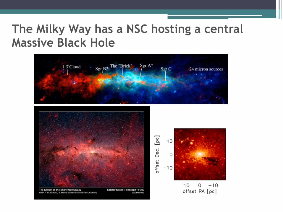
The Milky Way has a NSC hosting a central Massive Black Hole

NSCs form through cluster infall and/or in-situ star formation
• The in-situ star formation or gas model (Loose et al. 1982, Schinnerer et al. 2008, Milosavljevic 2004, Pflamm-Altenburg, Jan & Kroupa 2009), possibly in a disk like configuration.
• The cluster merger scenario (Tremaine et al. 1975, Ostriker 1988, Antonini, Capuzzo
Dolcetta, MB & Merritt 2012, Antonini 2013, Gnedin et al. 2013 and references therein).
Both processes can work in concert, and both could be important for the formation and evolution of NSCs.

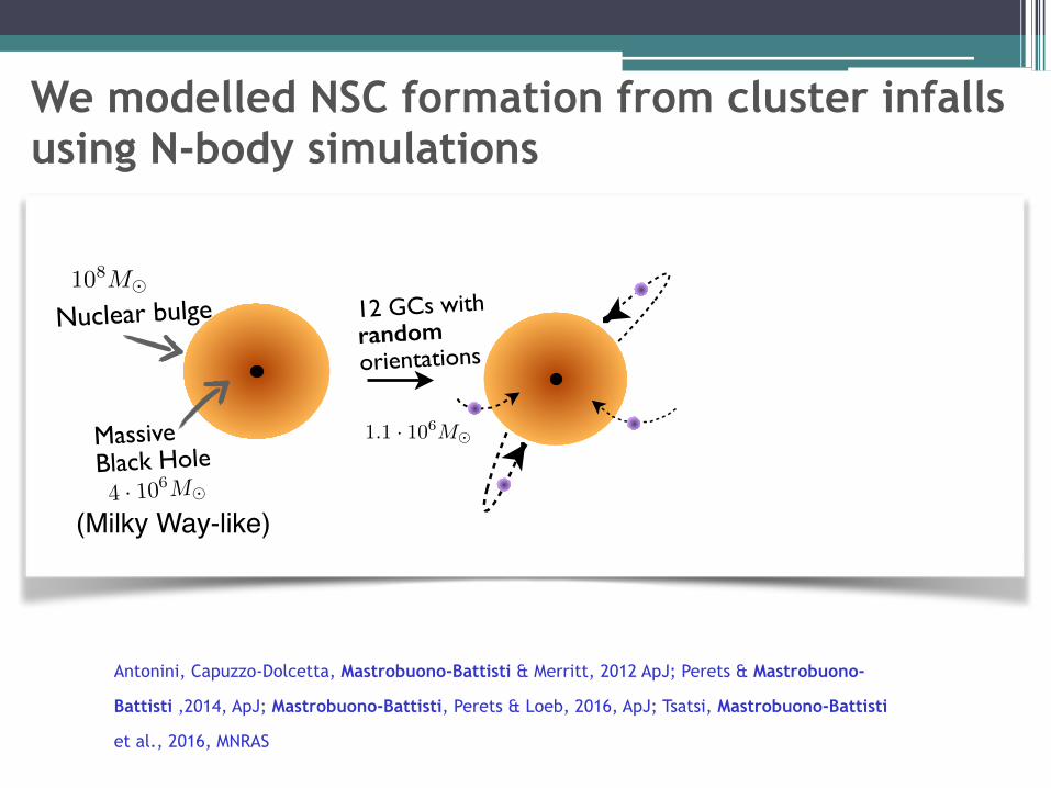
• Initially: only the nuclear bulge of the galaxy;
• An MBH (4x10⁶M⊙) is at the center of the galaxy;
• The NSC is build up by consecutive infalls;
• Collisional evolution of the NSC.
We modelled NSC formation from cluster infalls using N-body simulations
Antonini, Capuzzo-Dolcetta, Mastrobuono-Battisti & Merritt, 2012 ApJ; Perets & Mastrobuono-
Battisti ,2014, ApJ; Mastrobuono-Battisti, Perets & Loeb, 2016, ApJ; Tsatsi, Mastrobuono-Battisti
et al., 2016, MNRAS

• Initially: only the nuclear bulge of the galaxy;
• An MBH (4x10⁶M⊙) is at the center of the galaxy;
• The NSC is build up by consecutive infalls;
• Collisional evolution of the NSC.
We modelled NSC formation from cluster infalls using N-body simulations
4 · 106M�
108M�
Antonini, Capuzzo-Dolcetta, Mastrobuono-Battisti & Merritt, 2012 ApJ; Perets & Mastrobuono-
Battisti ,2014, ApJ; Mastrobuono-Battisti, Perets & Loeb, 2016, ApJ; Tsatsi, Mastrobuono-Battisti
et al., 2016, MNRAS
Nuclear bulge
Massive Black Hole
(Milky Way-like)
• Initially: only the nuclear bulge of the galaxy;
• An MBH (4x10⁶M⊙) is at the center of the galaxy;
• The NSC is build up by consecutive infalls;
• Collisional evolution of the NSC.
We modelled NSC formation from cluster infalls using N-body simulations
4 · 106M�
108M�12 GCs with random orientations
1.1 · 106M�
Antonini, Capuzzo-Dolcetta, Mastrobuono-Battisti & Merritt, 2012 ApJ; Perets & Mastrobuono-
Battisti ,2014, ApJ; Mastrobuono-Battisti, Perets & Loeb, 2016, ApJ; Tsatsi, Mastrobuono-Battisti
et al., 2016, MNRAS
Nuclear bulge
Massive Black Hole
(Milky Way-like)

• Initially: only the nuclear bulge of the galaxy;
• An MBH (4x10⁶M⊙) is at the center of the galaxy;
• The NSC is build up by consecutive infalls;
• Collisional evolution of the NSC.
We modelled NSC formation from cluster infalls using N-body simulations
4 · 106M�
108M�12 GCs with random orientations
1.1 · 106M�
Nuclear Star Cluster
1.5 · 107M�
~12 Gyr
Antonini, Capuzzo-Dolcetta, Mastrobuono-Battisti & Merritt, 2012 ApJ; Perets & Mastrobuono-
Battisti ,2014, ApJ; Mastrobuono-Battisti, Perets & Loeb, 2016, ApJ; Tsatsi, Mastrobuono-Battisti
et al., 2016, MNRAS
Nuclear bulge
Massive Black Hole
(Milky Way-like)

GCs decay and merge, forming the NSC: models based on Milky Way data
x (pc) x (pc)
y(pc
)
40
30
20
10
0
-10
-20
-30
-40
40
30
20
10
0
-10
-20
-30
-40
z(pc
)
-40 -30 -20 -10 0 10 20 30 40 -40 -30 -20 -10 0 10 20 30 40
• 12 GCs, initially at 20pc • 1.1x10⁶M⊙ each • ~800Myr between each infall
Antonini, Capuzzo-Dolcetta, Mastrobuono-Battisti &
Merritt (2012); Perets & Mastrobuono-Battisti (2014)

GCs decay and merge, forming the NSC: snapshots
Antonini, Capuzzo-Dolcetta, Mastrobuono-Battisti & Merritt 2012,
1st 2nd 3rd 4th
7th6th4th 8th
9th 10th 11th 12th

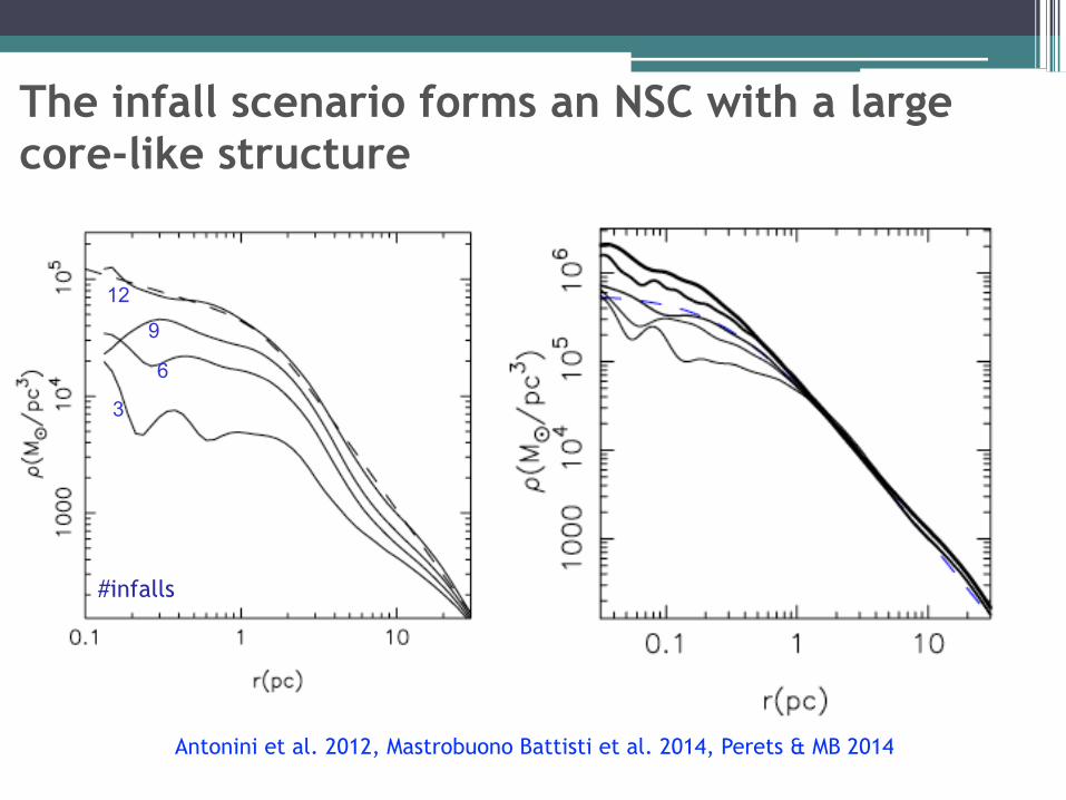
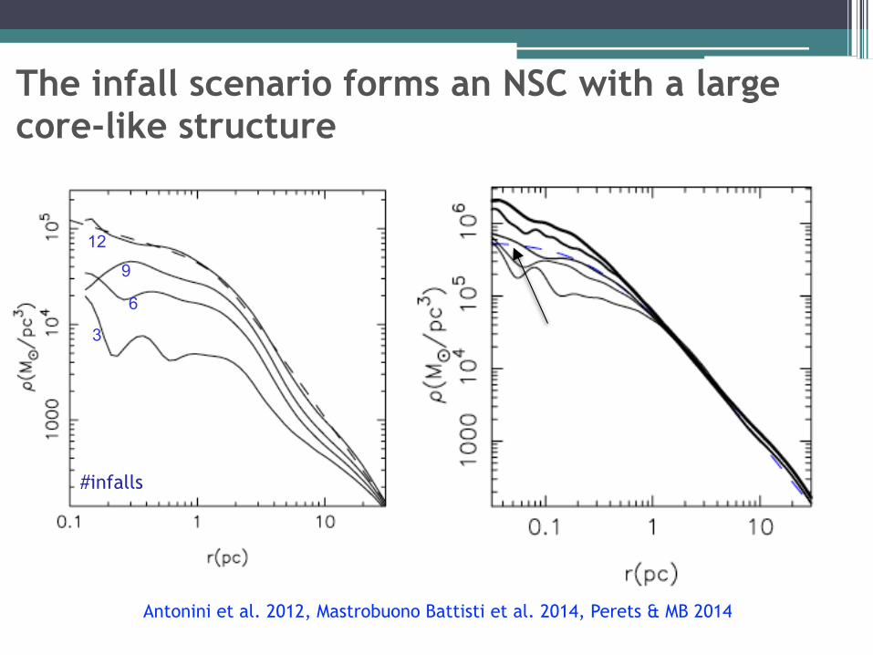
The infall scenario forms an NSC with a large core-like structure
Antonini et al. 2012, Mastrobuono Battisti et al. 2014, Perets & MB 2014
3
6
9
12
#infalls
The infall scenario forms an NSC with a large core-like structure
Antonini et al. 2012, Mastrobuono Battisti et al. 2014, Perets & MB 2014
3
6
9
12
#infalls
The infall scenario forms an NSC with a large core-like structure
Antonini et al. 2012, Mastrobuono Battisti et al. 2014, Perets & MB 2014
3
6
9
12
#infalls

The infall scenario forms an NSC with a large core-like structure
Antonini et al. 2012, Mastrobuono Battisti et al. 2014, Perets & MB 2014
3
6
9
12
10Gyr
#infalls

The infall scenario forms an NSC with a large core-like structure
Antonini et al. 2012, Mastrobuono Battisti et al. 2014, Perets & MB 2014
3
6
9
12
10Gyr
#infalls

The infall scenario forms an NSC with a large core-like structure
Antonini et al. 2012, Mastrobuono Battisti et al. 2014, Perets & MB 2014
3
6
9
12
10Gyr
20Gyr
#infalls

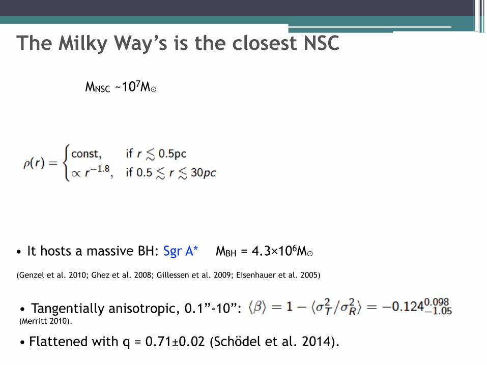
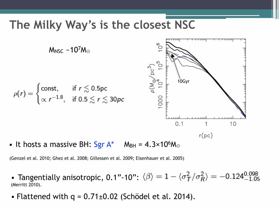
MNSC ~107M⊙
The Milky Way’s is the closest NSC
• It hosts a massive BH: Sgr A* MBH = 4.3×10⁶M⊙
• Tangentially anisotropic, 0.1”-10”: (Merritt 2010).
• Flattened with q = 0.71±0.02 (Schödel et al. 2014).
Schödel (2010)
(Genzel et al. 2010; Ghez et al. 2008; Gillessen et al. 2009; Eisenhauer et al. 2005)
MNSC ~107M⊙
The Milky Way’s is the closest NSC
• It hosts a massive BH: Sgr A* MBH = 4.3×10⁶M⊙
• Tangentially anisotropic, 0.1”-10”: (Merritt 2010).
• Flattened with q = 0.71±0.02 (Schödel et al. 2014).
(Genzel et al. 2010; Ghez et al. 2008; Gillessen et al. 2009; Eisenhauer et al. 2005)
MNSC ~107M⊙
The Milky Way’s is the closest NSC
• It hosts a massive BH: Sgr A* MBH = 4.3×10⁶M⊙
• Tangentially anisotropic, 0.1”-10”: (Merritt 2010).
• Flattened with q = 0.71±0.02 (Schödel et al. 2014).
(Genzel et al. 2010; Ghez et al. 2008; Gillessen et al. 2009; Eisenhauer et al. 2005)
10Gyr

Simulations vs Observations: Direct comparison with the
Milky Way NSC

ν
Feldmeier + 2014
σ
What do we learn from observations?
arcsec arcsec
arcsec
arcs
ec
arcs
ec
arcs
ec 1pc ~ 26’’

We can get similar maps for the simulated cluster

We can get similar maps for the simulated cluster

We can get similar maps for the simulated cluster

We can get similar maps for the simulated cluster

The real and simulated NSC look similar
arcsec arcsec arcsec
arcs
ec
arcs
ec
arcs
ec1pc ~ 26’’
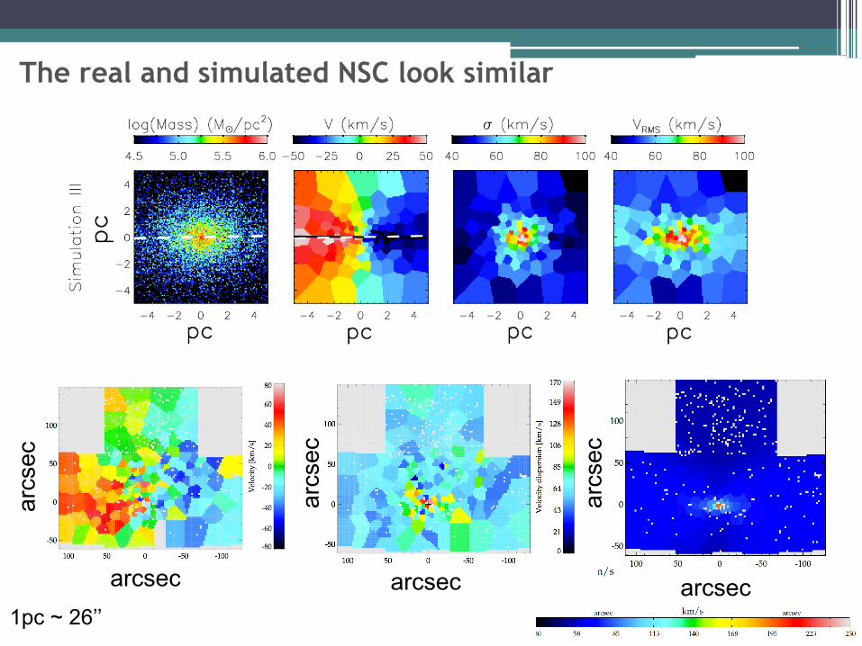
The real and simulated NSC look similar
arcsec arcsec arcsec
arcs
ec
arcs
ec
arcs
ec1pc ~ 26’’

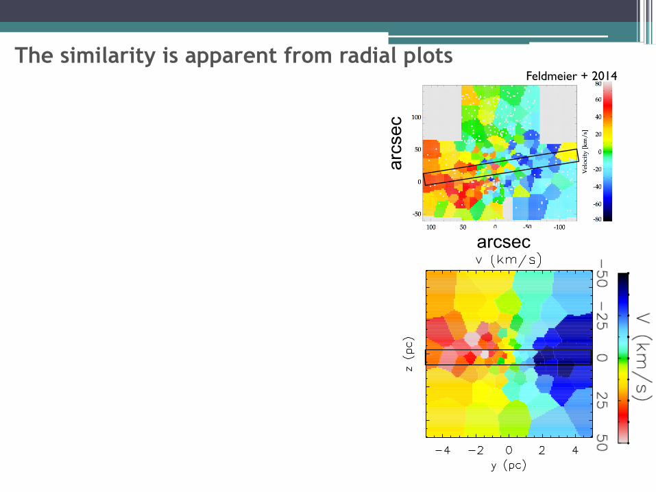
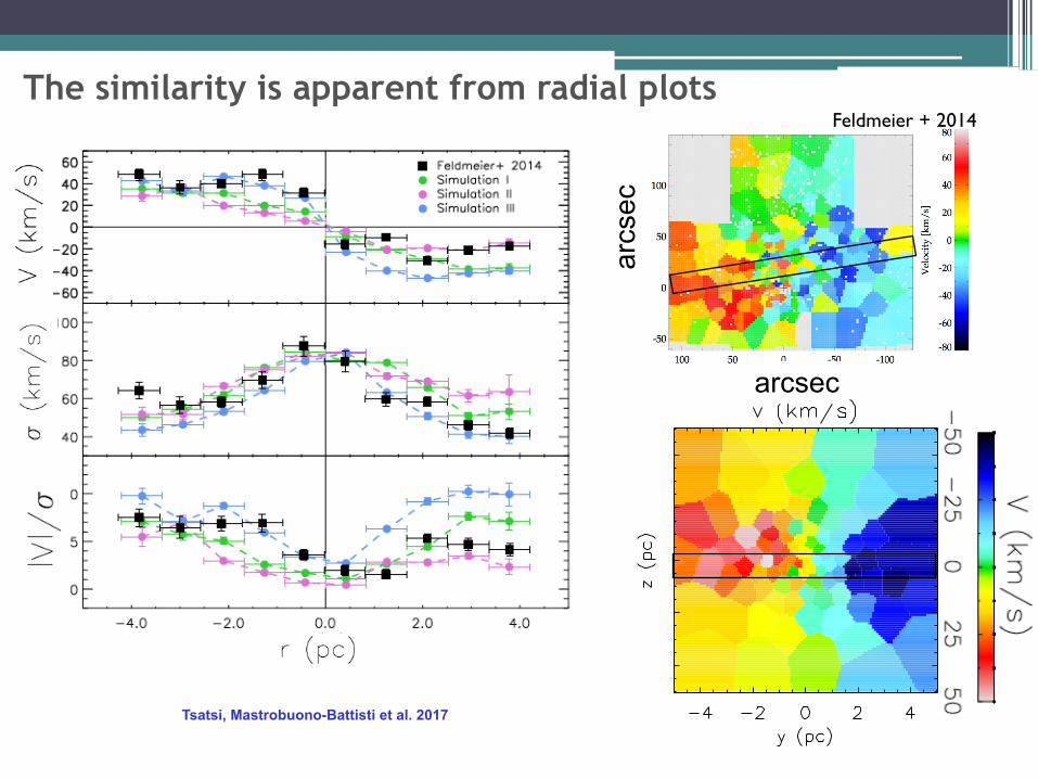
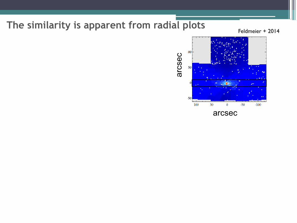
The similarity is apparent from radial plots
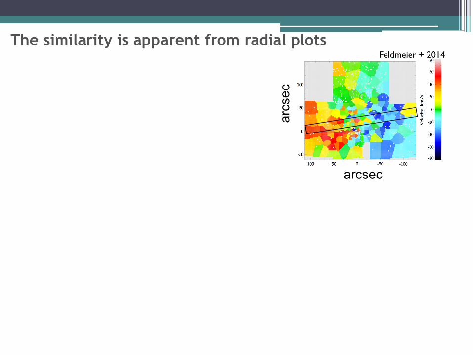
Feldmeier + 2014The similarity is apparent from radial plots
arcsec
arcs
ec
Feldmeier + 2014The similarity is apparent from radial plots
arcsec
arcs
ec
Feldmeier + 2014
Tsatsi, Mastrobuono-Battisti et al. 2017
The similarity is apparent from radial plots
arcsec
arcs
ec
The similarity is apparent from radial plots
Feldmeier + 2014The similarity is apparent from radial plots
arcsec
arcs
ec

Feldmeier + 2014The similarity is apparent from radial plots
arcsec
arcs
ec

Feldmeier + 2014The similarity is apparent from radial plots
arcsec
arcs
ec
Tsatsi, Mastrobuono-Battisti et al. 2017

Feldmeier + 2014The similarity is apparent from radial plots
arcsec
arcs
ec
Tsatsi, Mastrobuono-Battisti et al. 2017

Which role has the bulge?
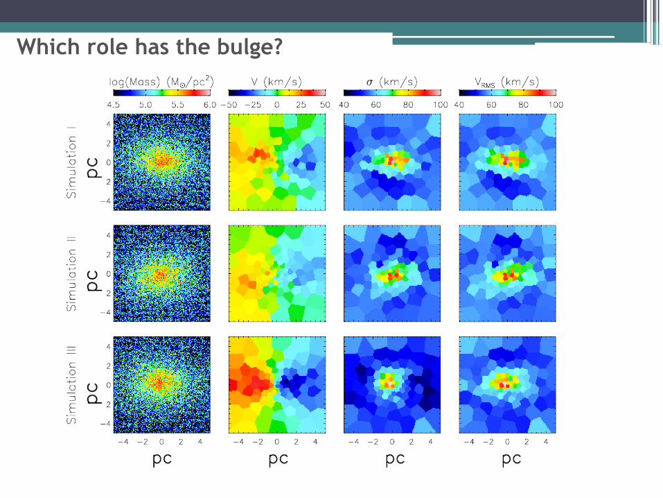
Which role has the bulge?

Kinematic profiles are still consistent
A&A 570, A2 (2014)
0.0 0.1 0.2 0.3 0.4 0.5 0.6COmag
3000
4000
5000
6000
7000
8000
Tef
f (K
)
SupergiantGiant
F0 F2 G0 G2 G5 G8 K0 K1 K2 K3
K4 K5 K7 M0 M1 M2 M3 M4 M5 M6
Fig. 7. Relationship between e↵ective temperature Te↵ in K and the COindex COmag for giant (triangle symbol) and supergiant (square symbol)stars of the IRTF Spectral Library (Rayner et al. 2009). Di↵erent coloursdenote a di↵erent spectral type. The black horizontal line marks 4800 K,the black vertical line marks COmag = 0.09.
parameters, the kinematic position angle PAkin, and kinematicaxial ratio qkin (= 1 � ✏kin). By default qkin is constrained to theinterval [0.1, 1], while we let PAkin unconstrained.
The result of the kinemetric analysis of the velocity mapfrom the cleaned data cube (Fig. 5) is listed in Table 2, andthe upper panel of Fig. 8 shows the kinemetry model velocitymap. From the axial ratio one can distinguish three families ofellipses. The three innermost ellipses form the first family, thenext seven ellipses build the second family, and the outermostfive ellipses form the third family.
For the two outer families the kinematic position anglePAkin is 4�15� Galactic east of north, with a median valueof 9�. However, the photometric position angle PAphot was mea-sured by Schödel et al. (2014) using Spitzer data to ⇠0�. Thismeans that there is an o↵set between PAphot and PAkin. Totest whether this o↵set could be caused by extinction from the20 km s�1 cloud (M-0.13-0.08, e.g. García-Marín et al. 2011) inthe Galactic south-west, we flag all bins in the lower right cor-ner as bad pixels and repeat the analysis, but the position angleo↵set remains. We test the e↵ect of Voronoi binning by runningkinemetry on a velocity map with S/N = 80. While the valuesof qkin for the second family are by up to a a factor two higherwith this binning, the PAkin fit is rather robust. We obtain a me-dian value for PAkin of 12.6� beyond a semi-major axis distanceof r ⇠ 4000. We conclude that the e↵ect of the binning can varythe value of the PAkin, but the PA o↵set from the Galactic planeis robust to possible dust extinction and binning e↵ects. Also ourcleaning of bright stars and foreground stars may cause a bias inthe PAkin measurements. For comparison we run the kinemetryon the velocity map of the full data cube (Fig. 4). In this casethere is higher scattering in the kinemetric parameters, causedby shot noise. However, beyond 3500 semi-major axis distancethe median PAkin is at 6.1�, i.e. the PA o↵set is retained. Thissmaller value could come from the contribution of foregroundstars, which are aligned along the Galactic plane. It could alsomean that bright stars are not as misaligned to the photometricmajor axis as fainter stars are. Young stars tend to be brighter,thus the integrated light likely samples an older population thanthe individual stars. Analysis of the resolved stars in the colourinterval 1.5m H � K 3.5m and in the radial range of 5000
V model
-60
-40
-20
0
20
40
60
arcs
ec
100 50 0 -50 -100arcsec
-80
-60
-40
-20
0
20
40
60
80
Vel
oci
ty [
km
/s]
V data
-100 -50 0 50 100arcsec
-50
0
50
100
arcs
ec
-80
-60
-40
-20
0
20
40
60
80
Vel
oci
ty [
km
/s]
Fig. 8. Upper panel: kinemetric model velocity map of the cleaned datacube. Black dots denote the best fitting ellipses. The model goes only tor ⇠ 10000 along the Galactic plane and to ⇠6000 perpendicular to it. TheVoronoi bin with the highest uncertainty was excluded from the model.Lower panel: the velocity map as in Fig. 5 shown in grayscale, the binsthat show rotation perpendicular to the Galactic plane are overplotted incolour scale.
to 10000 shows an o↵set in the rotation from the Galactic planeby (2.7±3.8)�. As previous studies focused on the brightest starsof the cluster, the PA o↵set of the old, faint population remainedundetected.
In the innermost family there is one ellipse with a positionangle of �81.5�, i.e. PAkin is almost perpendicular to the photo-metric position angle PAphot ⇡ 0�. This is caused by a substruc-ture at ⇠2000 north and south of Sgr A*, that seems to rotate onan axis perpendicular to the Galactic major axis. This feature ishighlighted in the lower panel of Fig. 8. North of Sgr A* wefind bins with velocities of 20 to 60 km s�1, while in the Galacticsouth bins with negative velocities around �10 to �30 km s�1 arepresent. The feature expands over several Voronoi bins north andsouth of Sgr A*. It extends over ⇠3500 (1.4 pc) along the Galacticplane, and ⇠3000 (1.2 pc) perpendicular to it.
This substructure also causes the small axial ratio valuesof the second family of ellipses between 3000 and 7000 in ourkinemetry model. All semi-minor axis distances from Sgr A*are below 2000, i.e. at smaller distances to Sgr A* than the per-pendicular substructure. Only the third family of ellipses, whichhas semi-major axis values above 7000, skips over this substruc-ture and reaches higher values of qkin.
To check if the perpendicular rotating substructure is real, weapply Voronoi binning with a higher S/N of 80 instead of 60, andobtain again this almost symmetric north-south structure. Alsowith a lower S/N of 50, the substructure appears in both datacubes. We also check the influence of the cleaning from brightstars on this feature using the cleaned maps with Kcut = 11m andKcut = 12m. The substructure remains also in these data cubes,independent of the applied binning. The fact that this feature per-sists independent on the applied magnitude cut, or binning, and
A2, page 8 of 20
Feldmeier et al. 2014
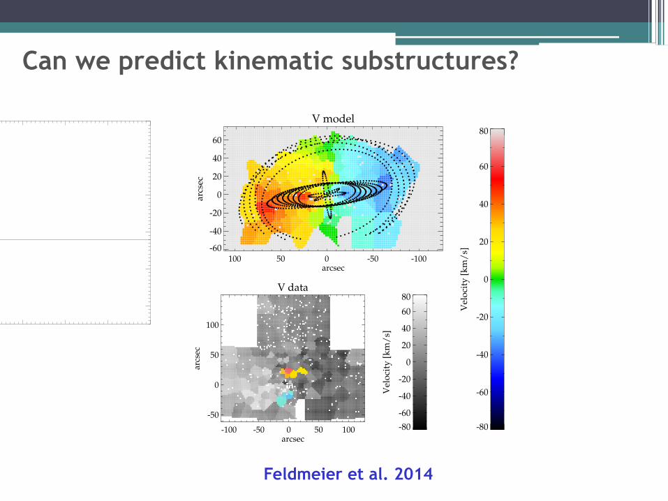
Can we predict kinematic substructures?
Feldmeier+2014
Tsatsi, Mastrobuono-Battisti et al., 2017
Can we predict kinematic substructures?

Feldmeier+2014
Kinemetry (Krajnovic’+2006)
Tsatsi, Mastrobuono-Battisti et al., 2017
Can we predict kinematic substructures?

Feldmeier+2014
Kinemetry (Krajnovic’+2006)
Tsatsi, Mastrobuono-Battisti et al., 2017
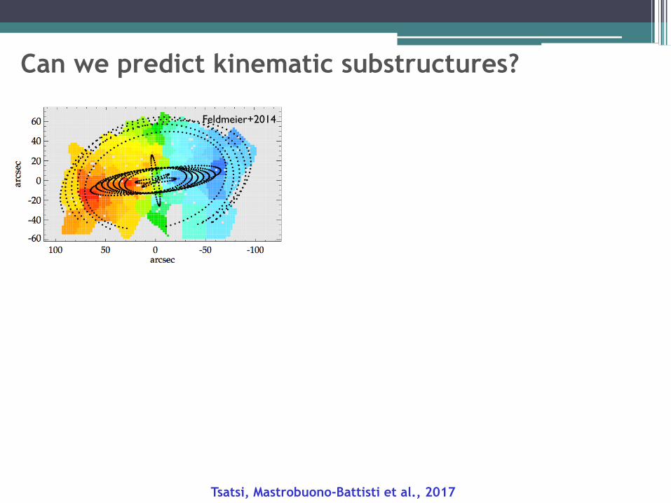
Can we predict kinematic substructures?
Created by a polar merger
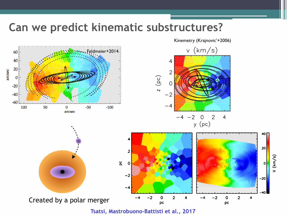
Feldmeier+2014
Kinemetry (Krajnovic’+2006)
Tsatsi, Mastrobuono-Battisti et al., 2017
Can we predict kinematic substructures?
Created by a polar merger

Feldmeier+2014
Kinemetry (Krajnovic’+2006)
Tsatsi, Mastrobuono-Battisti et al., 2017
Can we predict kinematic substructures?
Created by a polar merger
The effect of IMBHs on the formation and evolution of NSCs

IMBHs may be present in dense clusters and decay with them
Silk & Arons (1975): massive clusters may host an IMBH at their center:
• The merging model implies the presence of IMBHs in NSCs.
• We introduced an IMBH in each GC
Orbital radius of the last IMBH to fall in
The other 11 IMBHs
Mastrobuono-Battisti et al., 2014

The presence of IMBHs causes the NSC to have a steep cusp and to be strongly mass segregated
without IMBHs
with IMBHs
Mastrobuono-Battisti et al., 2014
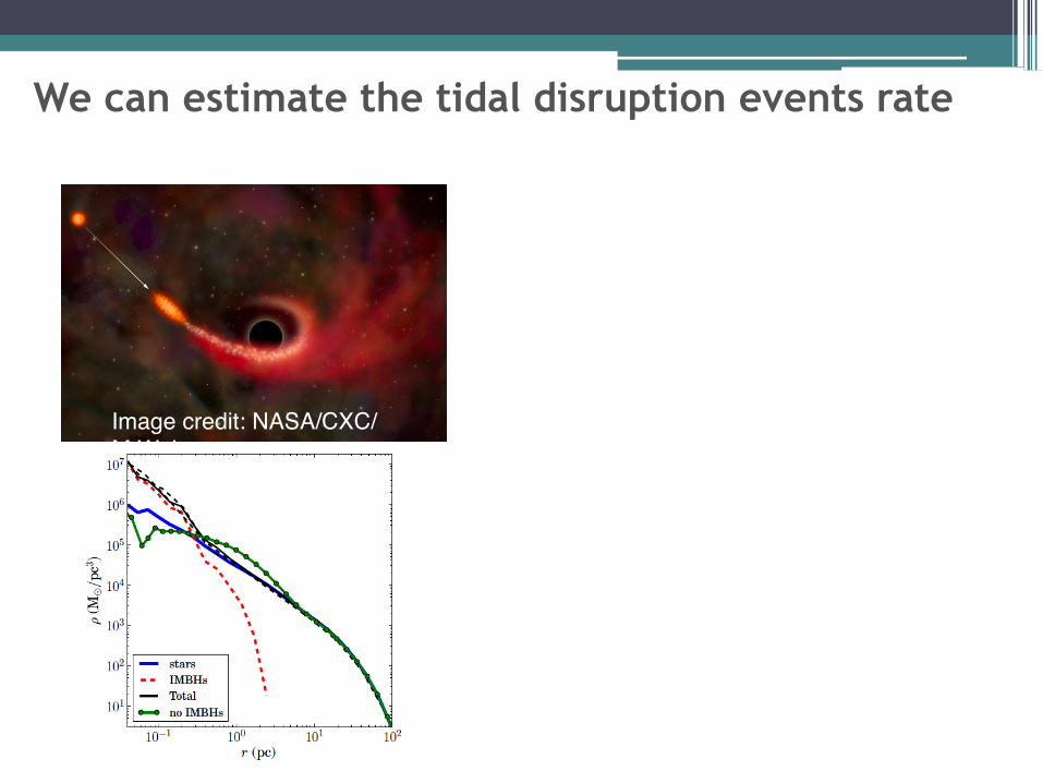
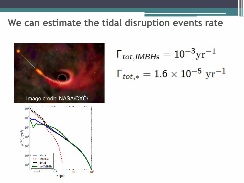
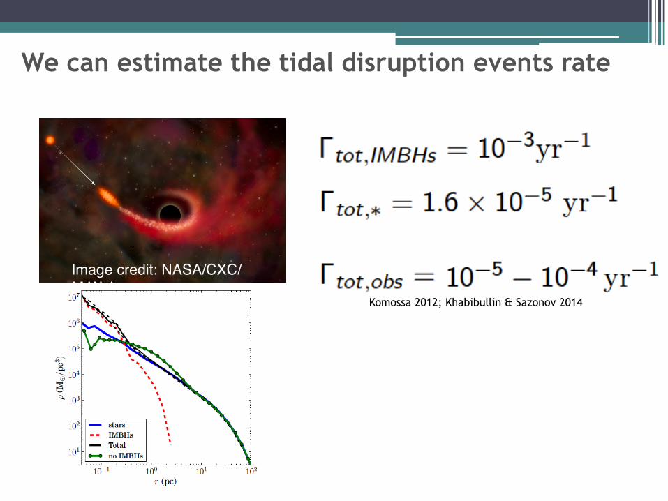
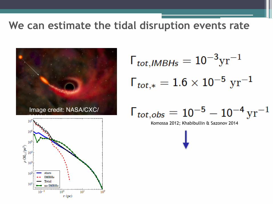
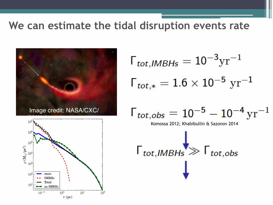
We can estimate the tidal disruption events rate
Image credit: NASA/CXC/M.Weiss

We can estimate the tidal disruption events rate
Image credit: NASA/CXC/M.Weiss
We can estimate the tidal disruption events rate
Image credit: NASA/CXC/M.Weiss
We can estimate the tidal disruption events rate
Image credit: NASA/CXC/M.Weiss
Komossa 2012; Khabibullin & Sazonov 2014
We can estimate the tidal disruption events rate
Image credit: NASA/CXC/M.Weiss
Komossa 2012; Khabibullin & Sazonov 2014

We can estimate the tidal disruption events rate
Image credit: NASA/CXC/M.Weiss
Komossa 2012; Khabibullin & Sazonov 2014
We can estimate the tidal disruption events rate
Image credit: NASA/CXC/M.Weiss
Komossa 2012; Khabibullin & Sazonov 2014

We can estimate the tidal disruption events rate
Image credit: NASA/CXC/M.Weiss
No IMBHs in NSCs?
Komossa 2012; Khabibullin & Sazonov 2014

Conclusions

• N-body simulations to study the merger scenario
Conclusions
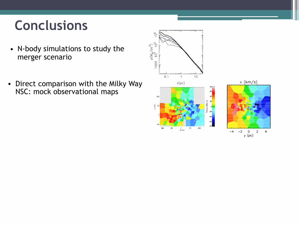
• N-body simulations to study the merger scenario
Conclusions
• Direct comparison with the Milky Way NSC: mock observational maps

• N-body simulations to study the merger scenario
Conclusions
• Direct comparison with the Milky Way NSC: mock observational maps
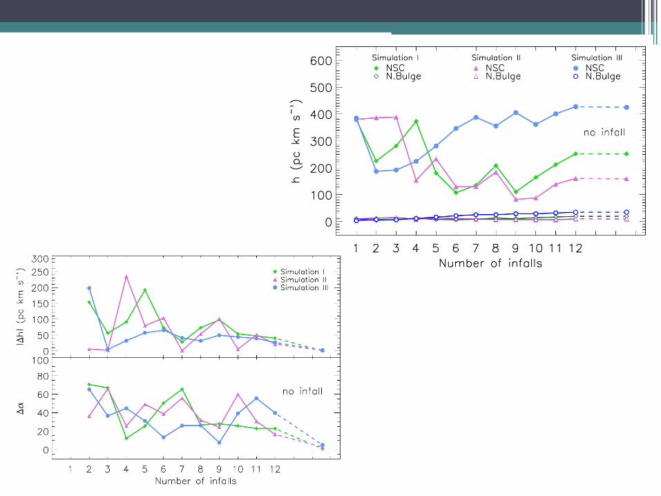
• The infall scenario reproduces most of the properties of the MW NSC, including its rotation

• N-body simulations to study the merger scenario
Conclusions
• Direct comparison with the Milky Way NSC: mock observational maps
• The infall scenario reproduces most of the properties of the MW NSC, including its rotation
• We also find kinematic substructures similar to the observed one: the infall scenario is really plausible!
• No IMBHs in NSCss? more observations needed!

• N-body simulations to study the merger scenario
Conclusions
• Direct comparison with the Milky Way NSC: mock observational maps
• The infall scenario reproduces most of the properties of the MW NSC, including its rotation
• Can we predict chemical properties? (Leaman, MB, work in prog.)
• We also find kinematic substructures similar to the observed one: the infall scenario is really plausible!
• No IMBHs in NSCss? more observations needed!
Thank you!