simulating rwm poster - columbia...
TRANSCRIPT

Kalman Filters to Reduce Noise Effects during External
Kink Control M. E. Mauel, J. Farrington, J. Bialek, O. Katsuro-Hopkins, A.
Klein, D. A. Maurer, G. A. Navratil, T. S. Pedersen
Columbia University
Annual Meeting of DPP-APSDenver, CO October 2005
AbstractMagnetic feedback control of the resistive wall mode in tokamaks use derivative (and proportional) gain in order to optimize stabilization (e.g. M. Okabayshi, et al., PoP2001; Y. Liu, et al., NF2004.) and to adjust the phase response during control of rotating kinks (A.Klein, et al., PoP2005.) Derivative gain amplifies noise and can lead to large and undesirable fluctuations in the feedback control current. In this poster, a recipe is presented for the implementation of a Kalman filter that tracks kink mode dynamics as recently described (M. E. Mauel, et al., NF2005.) Numerical simulations demonstrate the use of the control algorithm for various configurations of magnetic field sensors and control coils used in the HBT-EP device. By properly tracking both the wall and plasma modes, feedback control is maintained up to the ideal wall limit in rotating discharges in the presence of measurement noise.
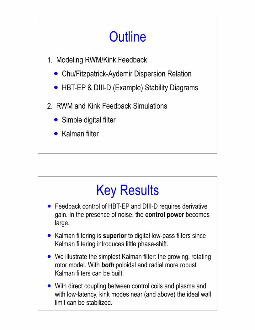
Outline
1. Modeling RWM/Kink Feedback
• Chu/Fitzpatrick-Aydemir Dispersion Relation
• HBT-EP & DIII-D (Example) Stability Diagrams
2. RWM and Kink Feedback Simulations
• Simple digital filter
• Kalman filter
Key Results• Feedback control of HBT-EP and DIII-D requires derivative
gain. In the presence of noise, the control power becomes large.
• Kalman filtering is superior to digital low-pass filters since Kalman filtering introduces little phase-shift.
• We illustrate the simplest Kalman filter: the growing, rotating rotor model. With both poloidal and radial more robust Kalman filters can be built.
• With direct coupling between control coils and plasma and with low-latency, kink modes near (and above) the ideal wall limit can be stabilized.

Non-Ideal Kinks (with Wall)
(! + i!)2K + (! + i!)D + "Wp +"W b
v!#!
w + "W"
v
!#!
w + 1= 0
Chu, et al., (1995)…
!
"#(! ! i!)2/!2
MHD$ %& '
Inertia
!
Viscosity& '$ %
"̄(!/! ! i) + (1 ! s̄)$ %& '
Kink
(
)*
WallMode& '$ %+
!
!w
(1 ! c) + 1
,
= 1
Equivalent to Fitzpatrick-Aydemir, (1996)…
Boozer/Coupling Parameters
s = !!Wp + !Wv,!
!Wv,!
= 2m ! nqa ! 1
m ! nqa
c = 1 !!Wv,!
!Wv,b
= 1 !1
!= 2
(a/b)2m
1 + (a/b)2m
s̄ "s
scrit
=
!
m ! nqa ! 1
m ! nqa
"
#
!
2
! ! 1
"
,
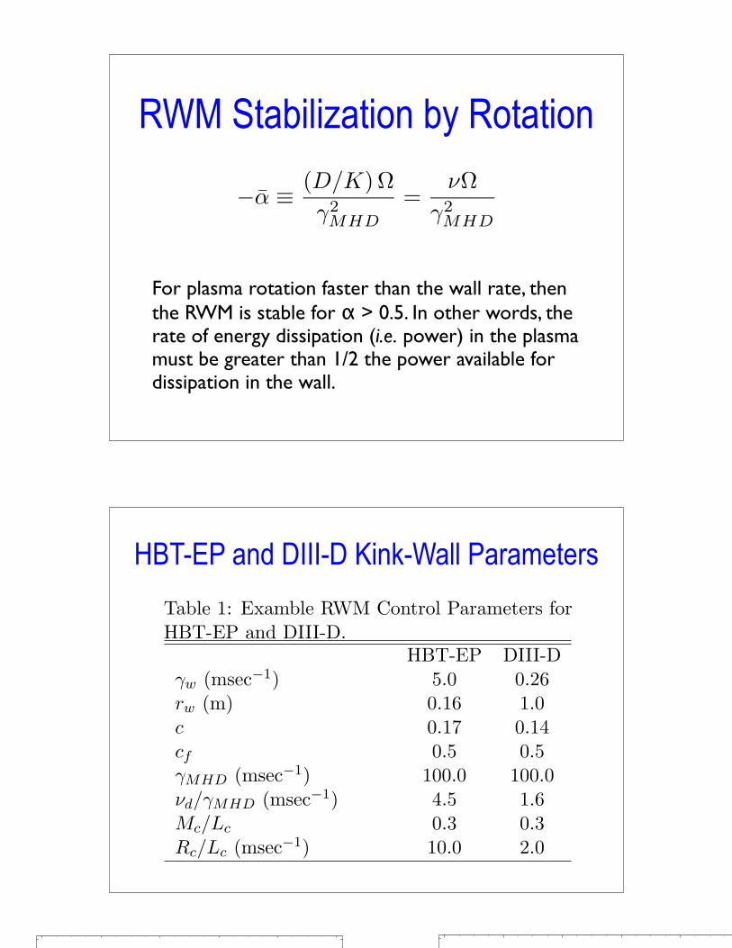
RWM Stabilization by Rotation
!!̄ "
(D/K) !
"2
MHD
=#!
"2
MHD
For plasma rotation faster than the wall rate, then the RWM is stable for ! > 0.5. In other words, the rate of energy dissipation (i.e. power) in the plasma must be greater than 1/2 the power available for dissipation in the wall.
HBT-EP and DIII-D Kink-Wall Parameters
Table 1: Examble RWM Control Parameters forHBT-EP and DIII-D.
HBT-EP DIII-D!w (msec!1) 5.0 0.26rw (m) 0.16 1.0c 0.17 0.14cf 0.5 0.5!MHD (msec!1) 100.0 100.0"d/!MHD (msec!1) 4.5 1.6Mc/Lc 0.3 0.3Rc/Lc (msec!1) 10.0 2.0
0 2 4 6 8 10
f !kHz"0
0.2
0.4
0.6
0.8
1
1.2
s
HBT!EP Stability Diagram
0 2 4 6 8 10
f !kHz"0
0.2
0.4
0.6
0.8
1
1.2
s
DIII!D Stability Diagram
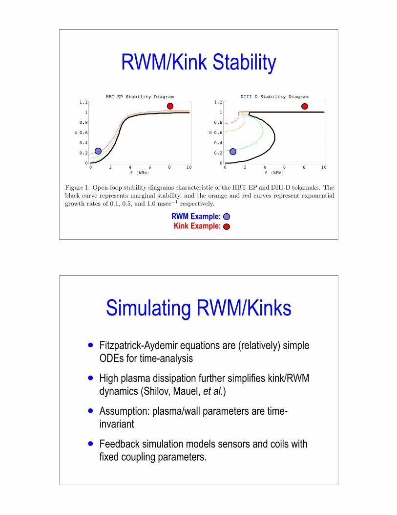
Figure 1: Open-loop stability diagrams characteristic of the HBT-EP and DIII-D tokamaks. Theblack curve represents marginal stability, and the orange and red curves represent exponentialgrowth rates of 0.1, 0.5, and 1.0 msec!1 respectively.
With this definition, the proportional gain has units of Volts per flux ! msec!1, and the deriva-tive gain is dimensionless. Also notice that the measured perturbed poloidal field, bp(rw), re-quires detectors at multiple toroidal locations. bp(rw)e!in!" is a complex phasor rotated by thecontroller by an amount #$. For simplicity, the toroidal rotation is the same for both the pro-portional and derivative gain terms. The feedback controller is defined by three real numbers,(Gp, Gd, #$). The closed-loop system response is defined by
!I"Gde
!i!"{0, 0, Mc/Lc} %m""· d%y"
dt= A" · %y" + Gpe
!i!"{0, 0, Mc/Lc} %m" · %y" , (11)
with %m" = 3(1" c)!1 # {2$
c, "(1 + c), 0} and (m, n) = (3, 1).The response of the magnetic control coil is an important consideration. When the instability
eigenvalue is slow, |!| % Rc/Lc, then the control coil responds in the “resistive limit”, &c &
4
RWM/Kink Stability
Table 1: Examble RWM Control Parameters forHBT-EP and DIII-D.
HBT-EP DIII-D!w (msec!1) 5.0 0.26rw (m) 0.16 1.0c 0.17 0.14cf 0.5 0.5!MHD (msec!1) 100.0 100.0"d/!MHD (msec!1) 4.5 1.6Mc/Lc 0.3 0.3Rc/Lc (msec!1) 10.0 2.0
0 2 4 6 8 10
f !kHz"0
0.2
0.4
0.6
0.8
1
1.2
s
HBT!EP Stability Diagram
0 2 4 6 8 10
f !kHz"0
0.2
0.4
0.6
0.8
1
1.2
s
DIII!D Stability Diagram
Figure 1: Open-loop stability diagrams characteristic of the HBT-EP and DIII-D tokamaks. Theblack curve represents marginal stability, and the orange and red curves represent exponentialgrowth rates of 0.1, 0.5, and 1.0 msec!1 respectively.
With this definition, the proportional gain has units of Volts per flux ! msec!1, and the deriva-tive gain is dimensionless. Also notice that the measured perturbed poloidal field, bp(rw), re-quires detectors at multiple toroidal locations. bp(rw)e!in!" is a complex phasor rotated by thecontroller by an amount #$. For simplicity, the toroidal rotation is the same for both the pro-portional and derivative gain terms. The feedback controller is defined by three real numbers,(Gp, Gd, #$). The closed-loop system response is defined by
!I"Gde
!i!"{0, 0, Mc/Lc} %m""· d%y"
dt= A" · %y" + Gpe
!i!"{0, 0, Mc/Lc} %m" · %y" , (11)
with %m" = 3(1" c)!1 # {2$
c, "(1 + c), 0} and (m, n) = (3, 1).The response of the magnetic control coil is an important consideration. When the instability
eigenvalue is slow, |!| % Rc/Lc, then the control coil responds in the “resistive limit”, &c &
4
RWM Example:Kink Example:
Simulating RWM/Kinks
• Fitzpatrick-Aydemir equations are (relatively) simple ODEs for time-analysis
• High plasma dissipation further simplifies kink/RWM dynamics (Shilov, Mauel, et al.)
• Assumption: plasma/wall parameters are time-invariant
• Feedback simulation models sensors and coils with fixed coupling parameters.
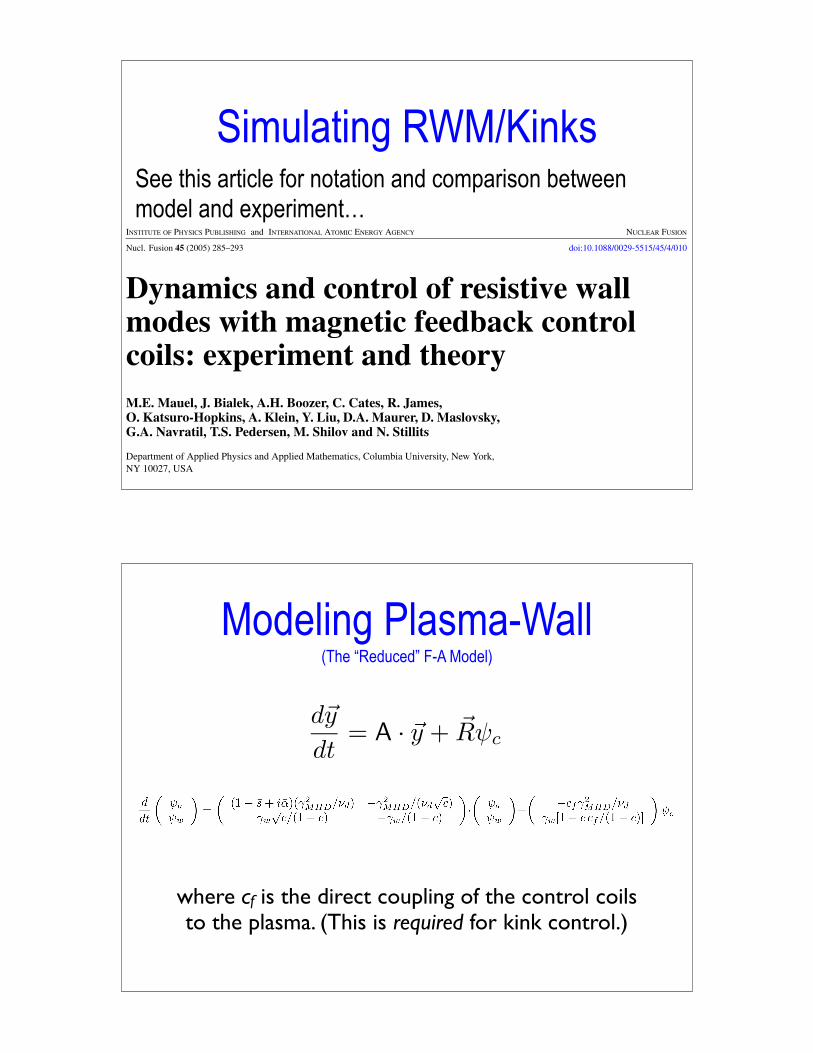
Simulating RWM/Kinks
INSTITUTE OF PHYSICS PUBLISHING and INTERNATIONAL ATOMIC ENERGY AGENCY NUCLEAR FUSION
Nucl. Fusion 45 (2005) 285–293 doi:10.1088/0029-5515/45/4/010
Dynamics and control of resistive wallmodes with magnetic feedback controlcoils: experiment and theoryM.E. Mauel, J. Bialek, A.H. Boozer, C. Cates, R. James,O. Katsuro-Hopkins, A. Klein, Y. Liu, D.A. Maurer, D. Maslovsky,G.A. Navratil, T.S. Pedersen, M. Shilov and N. Stillits
Department of Applied Physics and Applied Mathematics, Columbia University, New York,NY 10027, USA
Received 10 December 2004, accepted for publication 2 March 2005Published 1 April 2005Online at stacks.iop.org/NF/45/285
AbstractFundamental theory, experimental observations and modelling of resistive wall mode (RWM) dynamics and activefeedback control are reported. In the RWM, the plasma responds to and interacts with external current-carryingconductors. Although this response is complex, it is still possible to construct simple but accurate models forkink dynamics by combining separate determinations for the external currents, using the VALEN code, and forthe plasma’s inductance matrix, using an magnetohydrodynamics code such as DCON. These computations havebeen performed for wall-stabilized kink modes in the HBT-EP device, and they illustrate a remarkable feature ofthe theory: when the plasma’s inductance matrix is dominated by a single eigenmode and when the surroundingcurrent-carrying structures are properly characterized, then the resonant kink response is represented by a smallnumber of parameters. In HBT-EP, RWM dynamics are studied by programming quasi-static and rapid ‘phase-flip’changes of the external magnetic perturbation and directly measuring the plasma response as a function of kinkstability and plasma rotation. The response evolves in time, is easily measured, and involves excitation of boththe wall-stabilized kink and the RWM. High speed, active feedback control of the RWM using VALEN-optimizedmode-control techniques and high-throughput digital processors is also reported. Using newly installed control coilsthat directly couple to the plasma surface, experiments demonstrate feedback suppression of the kink instability inrapidly rotating plasmas near the ideal wall stability limit.
PACS numbers: 52.35.Py, 52.55.Fa
(Some figures in this article are in colour only in the electronic version)
1. Introduction
Among fusion’s significant accomplishments during the pastdecade is the improved understanding and control of long-wavelength kink instabilities that grow on the rate of resistivepenetration of a nearby conducting wall, !w. These slowlygrowing instabilities, called resistive wall modes (RWMs),appear when non-axisymmetric eddy currents in the walloppose, or wall-stabilize, fast ideal kink modes. When theRWM is controlled, tokamaks and spherical tori can operatewith high plasma pressure making possible advanced steady-state operating scenarios having good confinement and lowcurrent drive power requirements [1]. Stabilization of theRWM has been seen in tokamak experiments through sustainedplasma rotation [4] or by active feedback control [6, 7].Using the three-dimensional electromagnetic modelling code
VALEN [8], experiments have been realistically modelled,theoretical predictions have been benchmarked, and advancedcontrol systems have been designed for several toroidaldevices including HBT-EP [9], DIII-D, NSTX, JT-60SC,FIRE and ITER. Although tremendous progress has beenmade, important questions remain concerning the physics ofplasma dissipation, the torque applied between the RWMand the external conductors, the dynamics of wall-stabilizedkink modes, and the development of practical techniques thatinsure robust feedback control of the RWM [10].
This paper begins with a presentation of the fundamentaltheory behind the VALEN code and describes a generaleigenmode procedure that can be used to implement optimizedfeedback systems for the RWM. Quantitative modellingrequires (i) accurate information about the inductive couplingbetween current-carrying structures and coils that lie outside
0029-5515/05/040285+09$30.00 © 2005 IAEA, Vienna Printed in the UK 285
See this article for notation and comparison between model and experiment…
Modeling Plasma-Wall(The “Reduced” F-A Model)
d!y
dt= A · !y + !R"c
where cf is the direct coupling of the control coils to the plasma. (This is required for kink control.)

Control Coils
Lc
Mc
d!c
dt+
Rc
Mc
!c = Vc
(Embarrassingly easy, but, well, it’s easy!)This simple model illustrates noise and filtering.
Sensors
B̃p(rw, !, ") = !
!
bp(rw) eim(!!n"/m)"
bp(rw) = (3/rw)(1 ! c)!1 " {2#
c, !(c + 1)} · !y
br(rw) = (3/rw) ! {0, 1} · !y
For these examples, only poloidal field sensors are used.With both br and bp sensors and with both sine and cosine detectors, then
both unstable and stable modes can be used for a more robust Kalman filter.

“Smart-Shell” Controller
Vc = Gp!w + Gdd!w
dt
Only proportional and derivative gain needed for these examples.
Mode Control with Rotation
Vc = Gpe!in!"
rwbp(rw) + Gde!in!"
rwdbp(rw)
dt
Suppression of rotating external kink instabilities using optimized modecontrol feedback
Alexander J. Klein, David A. Maurer, Thomas Sunn Pedersen, Michael E. Mauel,Gerald A. Navratil, Cory Cates, Mikhail Shilov, Yuhong Liu, Nikolai Stillits, and Jim BialekPlasma Physics Laboratory, Columbia University, New York, New York 10027
!Received 14 December 2004; accepted 18 January 2005; published online 24 March 2005"
Rotating external kink instabilities have been suppressed as well as excited in a tokamak using
active magnetic coils that directly couple to the plasma through gaps in passive stabilizing
conducting shells that surround the plasma. The kink instability has a complex growth rate,
approximately !3+ i2!5""103 s!1, and is near the ideal wall stability limit when discharges areprepared with a rapid plasma current ramp and adjusted to have an edge safety factor near 3. The
active control coils are driven by a digital mode control feedback system that uses multiple
field-programmable gate arrays to analyze signals from 20 poloidal field sensors and achieve
high-speed feedback control. The feedback coil geometry used was designed to optimize feedback
effectiveness. Signal processing is of critical importance to optimize phase transfer functions for
control of rotating modes. © 2005 American Institute of Physics. #DOI: 10.1063/1.1868732$
External kink instabilities in tokamaks are driven by ra-
dial gradients of the plasma current,1and they set the stabil-
ity limit of high beta tokamak plasmas.2The stability of the
external kink depends significantly on the location and con-
ductivity of a wall surrounding the plasma. For a perfectly
conducting wall, the stability limit increases because eddy
currents in the wall generate fields to oppose the helical kink
perturbation. For any wall configuration, the ideal wall sta-
bility limit can be calculated using a three-dimensional !3D"electromagnetic code, like VALEN,
3and an ideal magneto-
hydrodynamic !MHD" stability code, like DCON.4 For awall with finite conductivity, the wall eddy currents decay,
and the external kink instability is called the resistive wall
mode !RWM" when the plasma is above the no-wall stabilitylimit but below the ideal wall stability limit.
5Although the
RWM grows slowly at a rate proportional to the eddy current
decay rate #w the RWM instability must be prevented in
order to operate steady-state tokamak reactors with both high
bootstrap current fraction and high fusion power density.6,7
Previous experiments have demonstrated stabilization of
the external kink with a conducting wall8and stabilization of
the RWM instability either by plasma rotation9,10
or by active
feedback control.11,12
In rotating plasma, plasma dissipation
stabilizes the RWM13,14
when the rate of dissipation exceeds
the rate at which energy is released from a slowly growing
!in proportion to #w" kink perturbation. Although the physicsof RWM stabilization due to rotation remains a subject of
study, recent measurements using the HBT-EP tokamak15
have shown rotationally stabilized kink perturbations to be
consistent with a semiempirical viscous model of
Fitzpatrick16in the high-dissipation regime. Near the ideal
wall stability limit, the RWM is stable when the plasma ro-
tation $ exceeds a critical value dependent upon the dissipa-
tion rate vd,
$crit = 2#MHD%#w/%d, !1"
where #MHD is the ideal MHD growth rate of the external
kink at the no-wall limit. The external kink growth rate for
rotating plasma at the ideal wall limit is #& i$+ !#MHD2 /%d"
"!S–1", where S is a normalized stability parameter. Kinkinstability results when S exceeds the ideal wall limit or
when S&1. S can be calculated with an ideal MHD code, itis defined as the ratio of the ideal kink perturbed energy 'Wcalculated without a wall, to the difference of the perturbed
vacuum energy when evaluated with and without an ideal
wall. High plasma dissipation slows the kink mode growth
rate from its usual value17by the factor %d /#MHD&1.
While feedback control of the slow RWM has been dem-
onstrated, feedback control near the ideal wall limit requires
consideration of both the marginally stable external kink that
rotates with the plasma $ and the RWM that rotates much
more slowly at a rate near #w($.16 Near the ideal wallstability limit in rotating plasma, the dominant frequency of
interest will be '#'($, and the active feedback controllermust be capable of high-speed control with low latency. In
addition, limitations to the feedback system arise from !1"the mutual inductive coupling between control and sensor
coils !leading to self-oscillations and ceilings on attainablegain, as well as noise", !2" coupling between the control coilsand the conducting shell !leading to finite response time ofthe system, as well as limiting the stability range over which
fixed feedback coefficients are effective18 ", and !3" coupling
between the sensor coils and conducting shells that slow the
response time of the feedback control fields. When these
limitations are eliminated, we describe feedback as “opti-
mized mode control.” Numerical modeling has predicted ex-
ternal kinks can then be feedback controlled up to the ideal
wall limit.3
In this paper, we report the first successful use of opti-
mized mode control of rotating external kink instabilities at
the ideal wall limit. External kink instabilities are excited in
PHYSICS OF PLASMAS 12, 040703 !2005"
1070-664X/2005/12!4"/040703/4/$22.50 © 2005 American Institute of Physics12, 040703-1
Downloaded 04 May 2005 to 128.59.145.17. Redistribution subject to AIP license or copyright, see http://pop.aip.org/pop/copyright.jsp
This is the controller demonstrated by Klein, et al.…
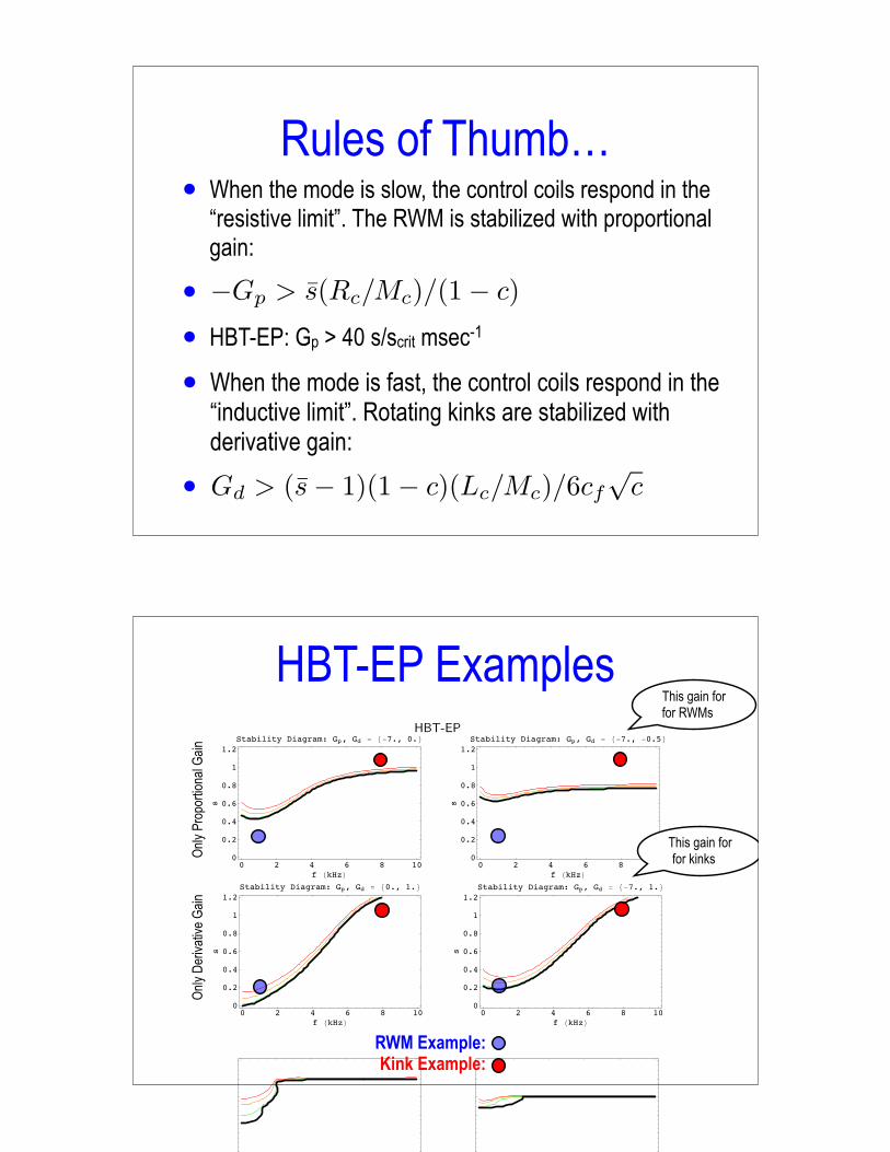
Rules of Thumb…• When the mode is slow, the control coils respond in the
“resistive limit”. The RWM is stabilized with proportional gain:
•
• HBT-EP: Gp > 40 s/scrit msec-1
• When the mode is fast, the control coils respond in the “inductive limit”. Rotating kinks are stabilized with derivative gain:
•
!Gp > s̄(Rc/Mc)/(1 ! c)
Gd > (s̄ ! 1)(1 ! c)(Lc/Mc)/6cf
"
c
HBT-EP ExamplesHBT-EP
0 2 4 6 8 10
f !kHz"0
0.2
0.4
0.6
0.8
1
1.2
s
Stability Diagram: Gp, Gd ! #"7., 0.$
0 2 4 6 8 10
f !kHz"0
0.2
0.4
0.6
0.8
1
1.2
s
Stability Diagram: Gp, Gd ! #"7., "0.5$
0 2 4 6 8 10
f !kHz"0
0.2
0.4
0.6
0.8
1
1.2
s
Stability Diagram: Gp, Gd ! #0., 1.$
0 2 4 6 8 10
f !kHz"0
0.2
0.4
0.6
0.8
1
1.2
s
Stability Diagram: Gp, Gd ! #"7., 1.$
DIII-D
0 2 4 6 8 10
f !kHz"0
0.2
0.4
0.6
0.8
1
1.2
s
Stability Diagram: Gp, Gd ! #"1., 0.$
0 2 4 6 8 10
f !kHz"0
0.2
0.4
0.6
0.8
1
1.2
s
Stability Diagram: Gp, Gd ! #"1.5, "0.5$
0 2 4 6 8 10
f !kHz"0
0.2
0.4
0.6
0.8
1
1.2
s
Stability Diagram: Gp, Gd ! #0., 0.5$
0 2 4 6 8 10
f !kHz"0
0.2
0.4
0.6
0.8
1
1.2
s
Stability Diagram: Gp, Gd ! #"1., 0.5$
Figure 2: Closed-loop stability diagrams (like Fig. 1) characteristic of the HBT-EP and DIII-Dtokamaks with various values for the proportional, Gp, and derivative, Gd, gains.
6
RWM Example:Kink Example:
This gain for for RWMs
This gain for for kinks O
nly
Pro
port
iona
l Gai
nO
nly
Der
ivat
ive
Gai
n

DIII-D Examples
HBT-EP
0 2 4 6 8 10
f !kHz"0
0.2
0.4
0.6
0.8
1
1.2
s
Stability Diagram: Gp, Gd ! #"7., 0.$
0 2 4 6 8 10
f !kHz"0
0.2
0.4
0.6
0.8
1
1.2
s
Stability Diagram: Gp, Gd ! #"7., "0.5$
0 2 4 6 8 10
f !kHz"0
0.2
0.4
0.6
0.8
1
1.2
s
Stability Diagram: Gp, Gd ! #0., 1.$
0 2 4 6 8 10
f !kHz"0
0.2
0.4
0.6
0.8
1
1.2
s
Stability Diagram: Gp, Gd ! #"7., 1.$
DIII-D
0 2 4 6 8 10
f !kHz"0
0.2
0.4
0.6
0.8
1
1.2
s
Stability Diagram: Gp, Gd ! #"1., 0.$
0 2 4 6 8 10
f !kHz"0
0.2
0.4
0.6
0.8
1
1.2
s
Stability Diagram: Gp, Gd ! #"1.5, "0.5$
0 2 4 6 8 10
f !kHz"0
0.2
0.4
0.6
0.8
1
1.2
s
Stability Diagram: Gp, Gd ! #0., 0.5$
0 2 4 6 8 10
f !kHz"0
0.2
0.4
0.6
0.8
1
1.2
s
Stability Diagram: Gp, Gd ! #"1., 0.5$
Figure 2: Closed-loop stability diagrams (like Fig. 1) characteristic of the HBT-EP and DIII-Dtokamaks with various values for the proportional, Gp, and derivative, Gd, gains.
6
RWM Example:Kink Example:
This gain for for RWMs
This gain for for kinks O
nly
Pro
port
iona
l Gai
nO
nly
Der
ivat
ive
Gai
n
Without Feedback…
0 10 20 30 40 50
msec
-0.006
-0.004
-0.002
0
0.002
0.004
0.006
DIII!D RWM: Measured Bp !No Feedback"
Bp
Bp
0 1 2 3 4
msec
-400000
-200000
0
200000
400000
DIII!D Kink: Measured Bp !No Feedback"
Bp
Bp
0 1 2 3 4 5 6 7msec
-1.5
-1
-0.5
0
0.5
1
1.5HBT!EP RWM: Measured Bp !No Feedback"
Bp
Bp
0 0.5 1 1.5 2msec
-2
-1
0
1
2
HBT!EP Kink: Measured Bp !No Feedback"
Bp
Bp
SineCosine
SineCosine

HBT-EP:Digital Feedback with 10!s Latency
0 1 2 3 4 5 6 7
msec
-0.00003
-0.00002
-0.00001
0
0.00001
0.00002
0.00003
0.00004
HBT!EP RWM: Measured Bp !Feedback"
Bp
Bp
0 1 2 3 4 5 6 7
msec
-0.0015
-0.001
-0.0005
0
0.0005
0.001
0.0015
0.002HBT!EP RWM: Control Power !Feedback"
Si
Co
0 0.5 1 1.5 2msec
-0.004
-0.002
0
0.002
0.004
HBT!EP Kink: Measured Bp !Feedback"
Bp
Bp
0 0.5 1 1.5 2msec
-0.04
-0.02
0
0.02
0.04
0.06
0.08
0.1HBT!EP Kink: Control Power !Feedback"
Si
Co
DIII-D:Digital Feedback with “20!s” Latency
0 0.5 1 1.5 2
msec
-0.01
-0.005
0
0.005
0.01
DIII!D Kink: Measured Bp !Feedback"
Bp
Bp
0 0.5 1 1.5 2
msec
-0.04
-0.02
0
0.02
0.04
0.06
0.08
0.1DIII!D Kink: Control Power !Feedback"
Si
Co
In[701]:=
!"#$!%#&#'()*+,"-!"#$!%#&#'().#$)/*+,"-
0 10 20 30 40 50msec
-0.00004
-0.00003
-0.00002
-0.00001
0
0.00001
0.00002
DIII!D RWM: Measured Bp !Feedback"
Bp
Bp
0 10 20 30 40 50msec
0
0.00002
0.00004
0.00006
0.00008
0.0001DIII!D RWM: Control Power !Feedback"
Si
Co
20!s OK for RWM
5!s Needed for Kink

Feedback With Random Noise (Toroidal Phase & Amplitude)
0 1 2 3 4 5 6 7
msec
-0.01
0
0.01
0.02
0.03
HBT!EP RWM: Measured Bp !Feedback"Noise#
Bp
Bp
0 1 2 3 4 5 6 7
msec
0
0.005
0.01
0.015
0.02HBT!EP RWM: Control Power !Feedback"Noise#
Si
Co
0 0.5 1 1.5 2
msec
-0.04
-0.02
0
0.02
HBT!EP Kink: Measured Bp !Feedback"Noise#
Bp
Bp
0 0.5 1 1.5 2
msec
-0.04
-0.02
0
0.02
0.04
0.06
0.08
0.1HBT!EP Kink: Control Power !Feedback"Noise#
Si
Co
Adding Low-Pass Digital Filters
b̄p[n] = b̄p[n! 1] +!t
"b
!bmp ! b̄p[n! 1]
"
d̄bp[n] = d̄bp[n! 1] +!t
"db
#b̄p[n]! b̄p[n! 1]
!t! d̄bp[n! 1]
$
For these examples "b = "bd = 5!t, and Vc[n+1] " Gb̄bp[n]+Gdd̄bp[n].

HBT-EP: Low-Pass Digital Filters
Filter phase-shift destabilizes kink…
0 0.5 1 1.5 2
msec
-2
-1
0
1
2
HBT!EP Kink: Measured Bp !Feedback"Noise"Filtered#
Bp
Bp
0 0.5 1 1.5 2
msec
-1.5
-1
-0.5
0
0.5
1
1.5
HBT!EP Kink: Filtered Bp !Feedback"Noise"Filter#
Bp
Bp
0 1 2 3 4 5 6 7
msec
-0.01
0
0.01
0.02
0.03
0.04
HBT!EP RWM: Measured Bp !Feedback"Noise"Filter#
Bp
Bp
0 1 2 3 4 5 6 7
msec
-0.01
-0.005
0
0.005
0.01
0.015
HBT!EP RWM: Filtered Bp !Feedback"Noise"Filter#
Bp
Bp
Improves RWM control…
Similar results for DIII-D.
Rudolf Emil Kalman (May 19, 1930 -) is most famous for his invention ofthe Kalman filter, a mathematical digital signal processing technique widelyused in control systems and avionics to extract meaning (a signal) fromchaos (noise).
Kalman’s ideas on filtering were initially met with scepticism. He had more success inpresenting his ideas, however, while visiting Stanley Schmidt at the NASA Ames ResearchCenter in 1967. This led to the use of Kalman filters during the Apollo program.
He was born in Budapest, Hungary. He obtained his bachelor’s (1953) and master’s(1954) degrees from MIT in electrical engineering. His doctorate (1957) was from Colum-bia University. His worked as Research Mathematician at the Research Institute forAdvanced Study, in Baltimore, from 1958-1964, Professor at Stanford University from1964-1971, and Graduate Research Professor, and Director, at the Center for Mathemati-cal System Theory, University of Florida, Gainesville from 1971 to 1992. Starting in 1973,he simultaneously filled the chair for Mathematical System Theory at the Swiss FederalInstitute of Technology, (ETH) Zurich.
He received the IEEE Medal of Honor (1974), the IEEE Centennial Medal (1984), theInamori foundation’s Kyoto Prize in High Technology (1985), the Steele Prize of the Amer-ican Mathematical Society (1987), and the Bellman Prize (1997).
He is a member of the National Academy of Sciences (USA), the National Academy ofEngineering (USA), and the American Academy of Arts and Sciences (USA). He is aforeign member of the Hungarian, French, and Russian Academies of Science. He hasmany honorary doctorates. This year’s recipient of Columbia’s Eggelston Prize!

Simple Kalman Filter: Predictor & Corrector
The “prediction” step is
x!n = A · xn"1 + un
P!n = A · Pn"1 · AT + Q
where x!n and P!n are predictions of the next step state vector and errorcovariance.
The “correction” step is
Kn = P!n · HT · (H · P!n · HT + R)"1
xn = x!n + Kn · (zmn "H · x!n)
Pn = (I"Kn · H) · P!nKn is the “Kalman Gain”. R is the measurement noise covariance. With
R large, the tracking is less sensitive to noise. With H = HT = I, these
are especially simple.
Simplest Kalman Filter: Rotating, Growing Rotor
Let xn = {bp[n] cos!n, bp[n] sin!n, bp[n!1] cos!n!1, bp[n!1] sin!n!1},then
A =
!
"""#
"{"k}2#t !#{"k}2#t 1 0#{"k}2#t "{"k}2#t 0 1
1 0 0 00 1 0 0
$
%%%&
representing a rotating, growing “rotor”. The complex growth rate, "k, is a
filter parameter. Does not have to be too close to actual mode.
Note: this is a single-mode approximation, because only two independent
measurements are available: bp cos! and bp sin!. If we had both poloidal
and radial sensors, then the Kalman model could be written in terms of s̄
and $̄.
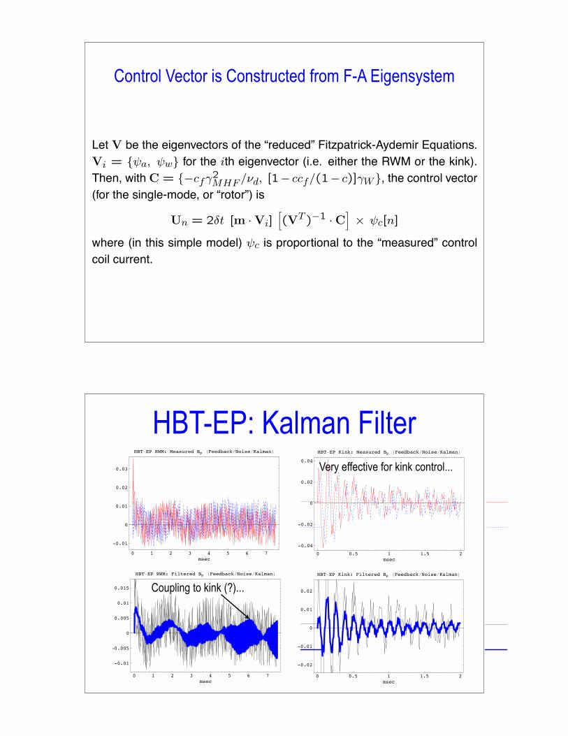
Control Vector is Constructed from F-A Eigensystem
Let V be the eigenvectors of the “reduced” Fitzpatrick-Aydemir Equations.
Vi = {!a, !w} for the ith eigenvector (i.e. either the RWM or the kink).
Then, withC = {!cf"2MHF/#d, [1! ccf/(1! c)]"W}, the control vector
(for the single-mode, or “rotor”) is
Un = 2$t [m · Vi]!(VT )!1 · C
"" !c[n]
where (in this simple model) !c is proportional to the “measured” control
coil current.
HBT-EP: Kalman Filter
0 1 2 3 4 5 6 7
msec
-0.01
0
0.01
0.02
0.03
HBT!EP RWM: Measured Bp !Feedback"Noise"Kalman#
Bp
Bp
0 1 2 3 4 5 6 7
msec
-0.01
-0.005
0
0.005
0.01
0.015
HBT!EP RWM: Filtered Bp !Feedback"Noise"Kalman#
Bp
Bp
0 0.5 1 1.5 2
msec
-0.04
-0.02
0
0.02
0.04
HBT!EP Kink: Measured Bp !Feedback"Noise"Kalman#
Bp
Bp
0 0.5 1 1.5 2
msec
-0.02
-0.01
0
0.01
0.02
HBT!EP Kink: Filtered Bp !Feedback"Noise"Kalman#
Bp
Bp
Coupling to kink (?)...
Very effective for kink control...
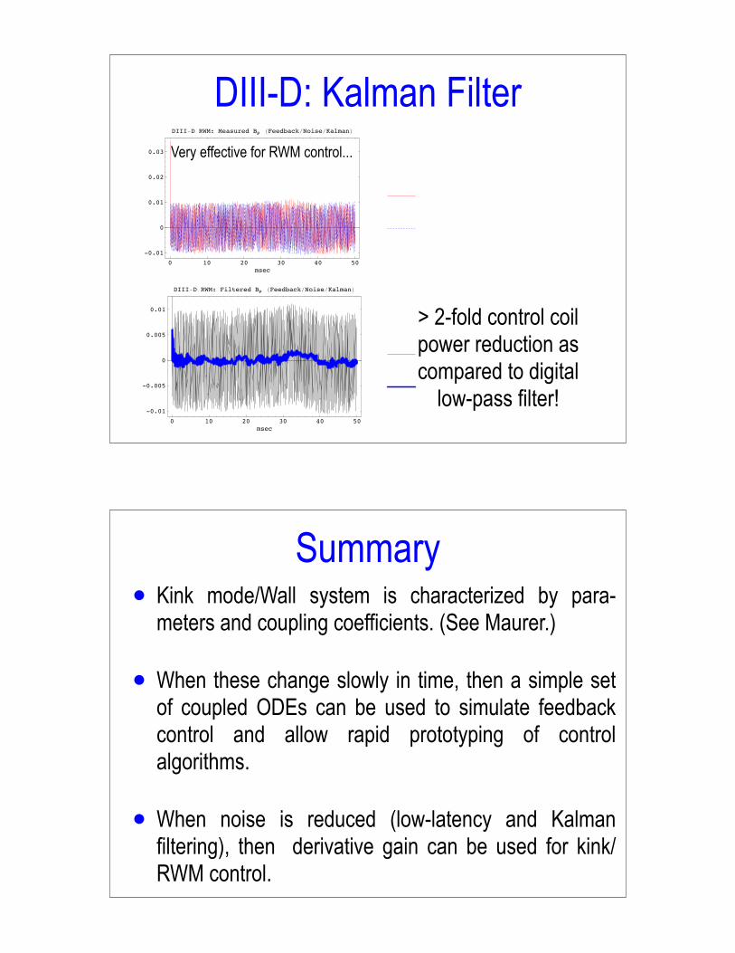
DIII-D: Kalman Filter
Very effective for RWM control...
0 10 20 30 40 50
msec
-0.01
0
0.01
0.02
0.03
DIII!D RWM: Measured Bp !Feedback"Noise"Kalman#
Bp
Bp
0 10 20 30 40 50
msec
-0.01
-0.005
0
0.005
0.01
DIII!D RWM: Filtered Bp !Feedback"Noise"Kalman#
Bp
Bp
> 2-fold control coil power reduction as compared to digital
low-pass filter!
Summary• Kink mode/Wall system is characterized by para-
meters and coupling coefficients. (See Maurer.)
• When these change slowly in time, then a simple set of coupled ODEs can be used to simulate feedback control and allow rapid prototyping of control algorithms.
• When noise is reduced (low-latency and Kalman filtering), then derivative gain can be used for kink/RWM control.