simulated versus measured energy performance of …...simulated versus measured energy performance...

NIST Special Publication 1182

Simulated versus Measured Energy

Performance of the NIST Net Zero

Energy Residential Test Facility

Design

Joshua Kneifel

William V. Payne

Tania Ullah

Lisa Ng

This publication is available free of charge from:

http://dx.doi.org/10.6028/NIST.SP.1182

NIST Special Publication 1182

Simulated versus Measured Energy

Performance of the NIST Net Zero

Energy Residential Test Facility

Design

Joshua Kneifel

Applied Economics Office

Engineering Laboratory

William V. Payne

Tania Ullah

Lisa Ng

Energy and Environment Division

Engineering Laboratory



March 2015

U.S. Department of Commerce

Penny Pritzker, Secretary

National Institute of Standards and Technology

Willie May, Acting Under Secretary of Commerce for Standards and Technology and Director

Certain commercial entities, equipment, or materials may be identified in this

document in order to describe an experimental procedure or concept adequately.

Such identification is not intended to imply recommendation or endorsement by the

National Institute of Standards and Technology, nor is it intended to imply that the

entities, materials, or equipment are necessarily the best available for the purpose.

National Institute of Standards and Technology Special Publication 1182

Natl. Inst. Stand. Technol. Spec. Pub. 1182, 95 pages (March 2015)



CODEN: NTNOEF

iii

Abstract

The National Institute of Standards and Technology (NIST) received funding through the

American Recovery and Reinvestment Act (ARRA) to construct a Net Zero Energy

Residential Test Facility (NZERTF). The initial goal of the NZERTF is to demonstrate

that a net-zero energy residential design can “look and feel” like a typical home in the

Gaithersburg area. The demonstration phase of the project was from July 2013 through

June 2014, during which it successfully demonstrated that the house performed at “net

zero,” or produced as much electricity as it consumed over the entire year.

The purpose of this report is twofold. The first is to compare the pre-demonstration phase

whole building energy simulation to the measured performance of the NZERTF during

the demonstration phase, which will identify where the measured performance deviates

from the simulated performance of the house in its design state. These variations may be

due to incorrect simulation assumptions (e.g., incorrect efficiency parameters) or faulty

demonstration phase operation control of the NZERTF itself (e.g., equipment failures).

The components of the NZERTF for which the simulation and measured performance

vary the most can be used as a “lessons learned” guide for other researchers to consider in

other low-energy house simulation efforts. The second purpose is to adjust the pre-

demonstration phase simulation specifications to better represent the actual performance

of the NZERTF during the demonstration phase. The adjustments will lead to the

development of a validated simulation model that can be used for analysis of “what-if”

scenarios, such as alternative configurations of equipment, occupancy activity/behavior,

building envelope options, or sensitivity analysis.

There is significant variation between the pre-demonstration phase simulation results and

measured demonstration phase performance. First, the initial simulation assumptions

were incorrect due to a lack of information on the specifications of the installed

equipment. Second, where information was lacking, conservative parameter values were

used in the model in order to not underestimate consumption. Third, there was an

inability to directly model some of the installed equipment in the software. Fourth, the

operation schedules and controls of the NZERTF were adjusted throughout the

preparation for the demonstration phase. Finally, there were faults and adjustments in the

operation of the NZERTF during the demonstration phase.

Keywords

Net zero energy construction; energy efficiency; residential building; whole building

energy simulation

v

Preface

This study was conducted by the Applied Economics Office (AEO) in the Engineering

Laboratory (EL) at the National Institute of Standards and Technology (NIST). The study

is designed to compare the pre-demonstration phase whole building energy simulation to

the measured energy performance during the demonstration phase of the Net Zero Energy

Residential Test Facility project, determine the reasons for any variations between the

simulated and measured performance, and develop a validated simulation that better

represents the performance of the NZERTF. The intended audience includes researchers

in the residential building sector concerned with net zero energy residential performance.

Disclaimer

The policy of the National Institute of Standards and Technology is to use metric units in

all of its published materials. Because this report is intended for the U.S. construction

industry that uses U.S. customary units, it is more practical and less confusing to include

U.S. customary units as well as metric units. Measurement values in this report are

therefore stated in metric units first, followed by the corresponding values in U.S.

customary units within parentheses.

vii

Acknowledgements

The author wishes to thank everyone involved in the NZERTF project. A special thanks

to Farhad Omar, Dr. Hunter Fanney, Brian Dougherty, Dr. Andrew Persily, Steven

Emmerich, Dr. William Healy, Mark Davis, Piotr Domanski, and Matthew Boyd from

NIST, Cathy Gates, Betsy Pettit, and Daniel Bergey from Building Science Corporation

(BSC), and Richard Raustad and the other EnergyPlus Help Desk team members for their

assistance in designing the simulation model. Thank you to everyone for their advice and

recommendations for the writing of this report, including Dr. Eric O’Rear and Dr. Robert

Chapman of EL’s Applied Economics Office, Dr. William Healy of EL’s Energy and

Environment Division, and Dr. Nicos S. Martys of EL’s Materials and Structural Systems

Division.

ix

Author Information

Joshua D. Kneifel

Economist


100 Bureau Drive, Mailstop 8603

Gaithersburg, MD 20899-8603

Tel.: 301-975-6857

Email: [email protected]

William V. Payne

Mechanical Engineer




Tel.: 301-975-6663


Tania Ullah

Mechanical Engineer




Tel.: 301-975-5433


Lisa Ng

Mechanical Engineer




Tel.: 301-975-4832


mailto:[email protected]




xi

Contents Abstract ............................................................................................................................. iii Preface ................................................................................................................................ v Acknowledgements ......................................................................................................... vii Author Information ......................................................................................................... ix List of Acronyms ........................................................................................................... xvii 1 Introduction ............................................................................................................... 1

1.1 Background and Purpose ...................................................................................... 1

1.2 Literature Review ................................................................................................. 1

1.3 Approach .............................................................................................................. 3

2 Pre-Demonstration Phase Assumptions .................................................................. 5 2.1 Geometry and Building Envelope ........................................................................ 5

2.2 Pre-Demonstration Adjustments to NZERTF Simulation ................................... 9

2.3 Systems, Occupancy, and Operation .................................................................. 10

2.3.1 Occupancy ............................................................................................................. 10

2.3.2 Lighting ................................................................................................................. 11

2.3.3 Non-HVAC Interior Equipment ............................................................................ 12

2.3.4 Heating, Ventilation, and Air Conditioning (HVAC) ........................................... 14

2.3.5 Domestic Hot Water .............................................................................................. 22

2.3.6 Solar Photovoltaic ................................................................................................. 29

3 Pre-Demonstration Phase Model Results ............................................................. 33 3.1 Total Electricity Consumption and Production .................................................. 33

3.2 MELs, Appliances, and Lighting ....................................................................... 34

3.3 HVAC, DHW, and Solar Systems ..................................................................... 36

3.3.1 HVAC Equipment ................................................................................................. 36

3.3.2 DHW and Solar Thermal System .......................................................................... 37

3.3.3 Solar Photovoltaic Generation ............................................................................... 40

4 Adjustments to Simulation Model ......................................................................... 43 4.1 Infiltration........................................................................................................... 43

4.2 MELs and Appliances ........................................................................................ 43

4.3 Lighting .............................................................................................................. 44

4.4 HVAC System .................................................................................................... 45

4.5 DHW and Solar Thermal Systems ..................................................................... 47

4.6 Occupancy .......................................................................................................... 51

4.7 Missing Experimental Data and Equipment Faults for the Demonstration Phase

52

5 Validated Model Results......................................................................................... 55 5.1 Total Electricity Consumption and Production .................................................. 55

5.2 Lighting .............................................................................................................. 57

5.3 MELs and Appliances ........................................................................................ 59

5.4 HVAC System .................................................................................................... 60

5.5 Domestic Hot Water Electricity Consumption................................................... 66

5.6 Domestic Water Consumption ........................................................................... 68

xii

5.7 Solar Photovoltaic Generation ........................................................................... 69

6 Limitations ............................................................................................................... 71 7 Discussion and Future Research............................................................................ 73 References ........................................................................................................................ 75

xiii

List of Figures

Figure 2-1 Location of Weather Station used for E+ Simulation ...................................... 5 Figure 2-2 BSC Architectural Massing Model and NZERTF as Built .............................. 6 Figure 2-3 Google SketchUp 3-D Representation of the E+ Model .................................. 6

Figure 2-4 Occupancy Density ........................................................................................ 11 Figure 2-5 HVAC System Layout ................................................................................... 17 Figure 2-6 Domestic Hot Water Heating System ............................................................ 23 Figure 2-7 Domestic Hot Water End Use Schedules – Fraction of Peak Flow ............... 28 Figure 3-1 Annual Electricity Consumption and Production (kWh) ............................... 33

Figure 3-2 Total Electricity Consumption by Category - kWh ....................................... 34 Figure 3-3 Appliances and Plug Loads (MELs) by Room – kWh ................................... 35 Figure 3-4 Lighting by Room – kWh .............................................................................. 35

Figure 3-5 Heating and Cooling Consumption by Month – kWh ................................... 36 Figure 3-6 HRV Electricity Consumption by Month - kWh ........................................... 37 Figure 3-7 DHW and Solar Loop Pump Electricity Consumption by Month – kWh ...... 38 Figure 3-8 DHW and Solar Loop Pump Electricity Consumption by Month – kWh ...... 39

Figure 3-9 Daily Water Consumption – Gallons ............................................................. 40 Figure 3-10 Total Electricity Consumption and Solar PV Production (kWh) - Monthly 41

Figure 4-1 Adjusted Domestic Hot Water Heating System ............................................. 48 Figure 4-2 Air Temperature, Total Heating Electricity Consumption, Auxiliary

Electricity Consumption, and Combined Heating COP – December 1, 2013 .................. 54

Figure 5-1 Annual Electricity Consumption and Production - kWh ............................... 55 Figure 5-2 Monthly Electricity Consumption and Production - kWh ............................. 56

Figure 5-3 Total Electricity Use by Month - kWh ........................................................... 57 Figure 5-4 Annual Lighting Electricity Use – kWh ......................................................... 58

Figure 5-5 Lighting Electricity Use by Month – kWh ..................................................... 59 Figure 5-6 Equipment Electricity Use - kWh .................................................................. 60 Figure 5-7 Heating and Cooling Electricity Consumption – kWh .................................. 61

Figure 5-8 Monthly Heating Electricity Consumption by Component – kWh ................ 62 Figure 5-9 Monthly Defrost Electricity Consumption – kWh ......................................... 63

Figure 5-10 Monthly Heat Pump Standby Electricity Consumption – kWh ................... 63 Figure 5-11 Updated Heating Electricity Consumption (2014) – kWh ........................... 64 Figure 5-12 Updated Heating Electricity Consumption by Component – kWh .............. 65

Figure 5-13 HRV Electricity Consumption by Month - kWh ......................................... 66 Figure 5-14 Heat Pump Water Heater and Pump Electricity Use (kWh) – Monthly ...... 67 Figure 5-15 DHW Tank Average Water Temperatures (°C) – Monthly ......................... 68 Figure 5-16 Daily DHW Water Consumption – Gallons per Day ................................... 69

Figure 5-17 Total Solar PV Electricity Production (kWh) - Monthly ............................. 70

xv

List of Tables

Table 2-1 Framing and Insulation ...................................................................................... 7 Table 2-2 Window Specifications ...................................................................................... 7 Table 2-3 Infiltration Rates ................................................................................................ 9

Table 2-4 Changes in NZERTF Assumptions ................................................................... 9 Table 2-5 Systems, Occupants, and Operating Conditions .............................................. 10 Table 2-6 Occupant Activity Level .................................................................................. 11 Table 2-7 Lighting Total Wattage by Room .................................................................... 12 Table 2-8 Appliance Wattage and Sensible and Latent Load Fractions .......................... 13

Table 2-9 Miscellaneous Electrical Load Wattage and Sensible and Latent Loads ........ 13 Table 2-10 Thermostat Setpoints ..................................................................................... 15 Table 2-11 Heat Recovery Ventilator .............................................................................. 16

Table 2-12 Zone Sizing Parameters ................................................................................. 17 Table 2-13 HVAC System Sizing Parameters ................................................................. 18 Table 2-14 HVAC Fan Parameters .................................................................................. 18 Table 2-15 Cooling Coil .................................................................................................. 19

Table 2-16 Cooling Coil Performance Curves................................................................. 19 Table 2-17 Heating Coil................................................................................................... 20

Table 2-18 Heating Coil Performance Curves ................................................................. 20 Table 2-19 Dehumidifier Parameters ............................................................................... 21 Table 2-20 Dehumidifier Performance Curves ................................................................ 22

Table 2-21 Solar Thermal Collector Parameters ............................................................. 24 Table 2-22 Storage Tank and Water Heater Tank Parameters ........................................ 25

Table 2-23 Heat Pump Water Heater Operational Parameters ........................................ 26 Table 2-24 Hot Water Heat Pump Coil Parameters ......................................................... 26

Table 2-25 Heat Pump Water Heater Fan and DHW Fan Parameters ............................. 27 Table 2-26 Domestic Hot Water Loop Pump Parameters ............................................... 27 Table 2-27 Domestic Hot Water Use and Thermal Load Fractions ................................ 29

Table 2-28 Solar Photovoltaic Panel Parameters ............................................................. 30 Table 2-29 Solar Photovoltaic Inverter Parameters ......................................................... 31

Table 4-1 Adjustments to Peak Wattage for Appliances and MELs ............................... 44 Table 4-2 Adjustments to Lighting Peak Wattage by Room ........................................... 45 Table 4-3 Changes in Cooling DX Coil Parameters ........................................................ 45

Table 4-4 Changes in Heating DX Coil Parameters ........................................................ 46 Table 4-5 Changes in Heat Recovery Ventilator Parameters .......................................... 47 Table 4-6 Changes in Dehumidifier Parameters .............................................................. 47 Table 4-7 Solar Thermal Collector Parameters ............................................................... 48

Table 4-8 Solar Loop Pump Parameters .......................................................................... 49 Table 4-9 Changes in Storage Tank and Hot Water Heater Tank Parameters................. 50 Table 4-10 Changes in Hot Water Heat Pump Coil Parameters ...................................... 50 Table 4-11 Domestic Hot Water Use and Thermal Load Fractions ................................ 51 Table 4-12 Domestic Hot Water Target Temperature ..................................................... 51

Table 4-13 Occupant Activity Level................................................................................ 52 Table 4-14 Missing Experimental Data ........................................................................... 52 Table 4-15 Equipment Faults ........................................................................................... 53

xvii

List of Acronyms

Acronym Definition

ACH Air Changes Per Hour

AEO Applied Economics Office

AMY Actual Meteorological Year

ARRA American Recovery and Reinvestment Act

ASHRAE American Society of Heating, Refrigerating and Air-Conditioning Engineers

BA Building America

BSC Building Science Corporation

BTP Building Technology Program

CFM Cubic Feet Per Minute

COP Coefficient of Performance

DHW Domestic Hot Water

DOE Department of Energy

DX direct expansion

E+ EnergyPlus

EERE Energy Efficiency and Renewable Energy

EL Engineering Laboratory

ELA Effective Leakage Area

ETL Electrical Testing Labs

FPW Fraction of Peak Wattage

FPF Fraction of Peak Flow

gpm gallons per minute

HVAC Heating, Ventilating, and Air Conditioning

HRV heat recovery ventilator

MEL Miscellanous Electric Load

NIST National Institute of Standards and Technology

NREL National Renewable Energy Laboratory

NZERTF Net Zero Energy Residential Test Facility

OC on center

ODB Outdoor Dry-Bulb

PCI Peripheral Component Interconnect

xviii

Acronym Definition

PXI Peripheral Component Interconnect Extensions for Instrumentation

PV Photovoltaic

SHGC Solar Heat Gain Coefficient

TMY Typical Meteorological Year

VT Visual Transmittance

1

1 Introduction

1.1 Background and Purpose

The National Institute of Standards and Technology (NIST) received funding through the

American Recovery and Reinvestment Act (ARRA) to construct a Net Zero Energy Residential

Test Facility (NZERTF). The initial goal of the NZERTF is to demonstrate that a net-zero energy

residential design can “look and feel” like a typical home in the Gaithersburg area. The

demonstration phase of the project was from July 2013 through June 2014, during which it

successfully demonstrated the house performed at “net zero,” or produced as much electricity as

it consumed over the entire year.

The purpose of this report is twofold. The first is to compare the pre-demonstration phase whole

building energy simulation to the measured performance of the NZERTF during the

demonstration phase, which will identify where the measured performance deviates from the

simulated performance of the house in its design state. These variations may be due to incorrect

simulation assumptions (e.g., incorrect efficiency parameters) or faulty demonstration phase

operation control of the NZERTF itself (e.g., equipment failures). The components of the

NZERTF for which the simulation and measured performance vary the most can be used as a

“lessons learned” guide for other researchers to consider in other low-energy house simulation

efforts. The second purpose is to adjust the pre-demonstration phase simulation specifications to

better represent the actual performance of the NZERTF during the demonstration phase. The

adjustments will lead to the development of a validated simulation model that can be used for

analysis of “what-if” scenarios, such as alternative configurations of equipment, occupancy

activity/behavior, building envelope options, or sensitivity analysis.

1.2 Literature Review

The Department of Energy’s (DOE) Building Technologies Program within the Office of Energy

Efficiency and Renewable Energy is responsible for funding research at the national laboratories

for the Building America (BA) program. The Building America (BA) program has been at the

forefront of research of low-energy single-family housing design through a variety of outlets,

including the BA Best Practices Series, case studies for new construction and retrofits, and

technical reports and fact sheets. Hendron and Engebrecht (2010) defines the BA house protocols

to be implemented when simulating house energy performance.

Kneifel (2012) defines the assumptions and parameters for an EnergyPlus (E+) whole building

energy simulation (DOE 2013) based on the NZERTF construction and equipment specifications

to forecast the energy performance during the demonstration phase of the NZERTF project, both

in aggregate as well as at the individual occupant and equipment level. The results show that the

NZERTF design will not only reach net-zero performance, but produce significant excess

electricity for an entire year using Typical Meteorological Year (TMY) weather data.

2

Kneifel (2013) uses the E+ simulation model developed in Kneifel (2012), adjusts some

parameters in the model based on new information regarding the NZERTF’s construction and

intended operation, and compares the energy performance of the NZERTF design to a

comparable Maryland code-compliant building design. The analysis includes a total of eleven

E+ simulations, starting with the Maryland code-compliant design and then adding energy

efficiency measures incrementally until all measures are included to reach the NZERTF design.

This approach allows for a comparison across energy efficiency measures to determine the

incremental impact for each energy efficiency measure on energy consumption. The NZERTF

leads to a reduction of 60 % in energy consumption (118 % in net energy consumption) relative

to the 2012 International Energy Conservation Code (IECC) design while doing a better job at

controlling the indoor environment in terms of temperature and relative humidity.

Kneifel (2014) compares the life-cycle cost performance of the NZERTF design to a comparable

Maryland code-compliant building design using the results from the NZERTF E+ simulation

defined in Kneifel (2013), local utility electricity rate schedules, and a contractor report

estimating the associated construction costs. The combination of initial construction costs and

future energy costs are used to estimate the total present value costs of constructing and

operating the NZERTF relative to the Maryland code-compliant house design. The NZERTF is

more costly to build, but saves the homeowner money in energy costs and increases the market

value of the home at resale. Assuming the NZERTF is purchased with a 30-year mortgage at

4.5 % and a 20 % down payment, the home owner would realize net savings of $41 714, or a

5.6 % adjusted internal rate of return.

Pettit et al. (2015) describes the general approach implemented in the design of the NZERTF,

which reduces energy use through methods that are consistent with a homeowner’s means and

way of life using available technologies, using on-site generation of energy for the energy

required after energy consumption has been reduced as much as is feasible. The report presents

and discusses the ten general principles for the design of net-zero energy capable houses, and

then describes the strategies implemented and design and construction details specifically related

to the NZERTF. This provides a concrete example of a net-zero capable house for which the

development of the design is consistent with the ten underlying principles.

Fanney et al. (2015) summarizes the design of the NZERTF and operation of the facility during

its one-year demonstration phase (July 2013 through June 2014). The article includes

descriptions of the architectural design and construction of the NZERTF, the virtual family that

resides in the NZERTF, the instrumentation developed to control and monitor activity and

electricity consumption within the facility, presents measured performance data from the

demonstration phase, and explains the key lessons learned throughout the process of operating

such a complex facility continuously for an entire year.

3

1.3 Approach

This report compares the pre-demonstration phase E+ simulation to the measured performance

of the NZERTF during the demonstration phase using actual weather data, determines the

variations in energy performance, and adjusts the simulation model to better represent the

measured performance of the NZERTF. The pre-demonstration phase simulation results are

obtained from the E+ simulation model defined in Kneifel (2013), which is the most up-to-date

model that was developed before the beginning of the demonstration phase. The measured

performance data for the demonstration phase are obtained and compiled by NIST’s building

component expert(s) for each building system (Davis et al. 2014, Fanney et al. 2015). By

comparing annual and monthly consumption values for the simulation estimate and measured

performance, the reasons for the differences can be identified. These reasons include the

following:

Lack of information on the specifications of the installed equipment

Usage of conservative parameter values where information is lacking in order to not

underestimate consumption

Inability to directly model some of the installed equipment

Adjustment of operation schedules and controls of the NZERTF during preparation for

the demonstration phase

Faults and adjustments in the operation of the NZERTF during the demonstration phase

The appropriate adjustments are then incorporated into the E+ simulation model from Kneifel

(2013) and rerun to see how those changes impacted the performance of the simulation model

relative to the measured performance.

5

2 Pre-Demonstration Phase Assumptions

The E+ software was chosen to simulate the whole building energy performance. As in Kneifel

(2012) and Kneifel (2013), the simulations are run using a one-minute timestep. However, the

Actual Meteorological Year (AMY) weather file for the NZERTF demonstration phase (July 1,

2013 through June 30, 2014) for the KGAI weather station (Weather Analytics 2014) located

less than 11 km (7 miles) from the NIST campus as shown in Figure 2-1 is used in place of the

TMY file used in Kneifel (2012) and Kneifel (2013). The use of the AMY file leads to

simulation results that are directly comparable to the measured performance because the weather

used to create the results are for the same weather conditions.

Figure 2-1 Location of Weather Station used for E+ Simulation

The general assumptions required by E+ are described in detail in Kneifel (2012) while the

changes made to the simulation in Kneifel (2013) are shown in Section 2.2.

2.1 Geometry and Building Envelope

The dimensions specified in BSC (2009) and shown in the architectural massing model in Figure

2-2 are used along with Google SketchUp and National Renewable Energy Laboratory’s (NREL)

Legacy Open Studio plug-in to construct the building geometry of the NZERTF. Total

conditioned floor area of the E+ model is 284.6 m2 (3063 ft2). Actual conditioned floor area of

the NZERTF is 251.7 m2 (2709 ft2). There are two reasons the conditioned floor area of the

simulation model is 32.9 m2 (354 ft2) greater than the actual house design. First, the E+ model

does not account for the open foyer/stairway, which is approximately 19.0 m2 (204 ft2). Second,

6

the gable walls (west wall and east wall) of the 2nd floor have built in storage under the gable,

which decreases the conditioned floor area by approximately 14.3 m2 (154 ft2). These two

aspects of the model account for approximately 33.3 m2 (358 ft2), which decreases the

conditioned floor area to 251.3 m2 (2705 ft2) or a difference of only 0.4 m2 (4 ft2). Even though

these two aspects of the house are not considered finished floor area, their volume of space will

be conditioned.

Figure 2-2 BSC Architectural Massing Model and NZERTF as Built

Figure 2-3 shows the Google SketchUp three-dimensional geometry of the E+ model for the

NZERTF. The model includes seven separate zones with three actively conditioned (1st floor, 2nd

floor, and basement), three inactively conditioned zones – a.k.a. within the conditioned space

without ductwork to the space (open web joist space between the 1st and 2nd floors, main attic,

and living room attic) -, and one unconditioned zone (patio). The front porch and detached

garage with the covered walkway are all treated as shading surfaces, which block sunlight but do

not impact the thermal performance of the building envelope.

Figure 2-3 Google SketchUp 3-D Representation of the E+ Model

The NZERTF design adds energy efficiency measures to each aspect of the building envelope

listed in Table 2-1, Table 2-2, and Table 2-3: framing, wall, roof, fenestration, and infiltration.

The NZERTF is constructed using “advanced framing,” which uses 5.1 cm x 15.2 cm (2 in x

7

6 in) 61.0 cm (24 in) on center (OC) framing instead of the common practice of 5.1 cm x

10.2 cm (2 in x 4 in) 40.6 cm (16 in) OC framing (Lstiburek 2010). The thicker framing allows

for greater levels of insulation within the wall cavity while decreasing the amount of wood

required for framing the house, making it easier to increase the thermal performance of the

building envelope.

Table 2-1 Framing and Insulation

Insulation NZERTF

Framing 5.1 cm x 15.2 cm (2 in x 6 in) 61.0 cm (24 in) OC

Exterior Wall

RSI-3.5 + 4.2 (R-20 + 24)

Basement Wall RSI-3.9 (R-22)

Roof RSI-7.9 + 5.3 (R-45 + 30)

Note 1: Interior + Exterior R-Value

The NZERTF design uses advanced framing and adds an additional RSI-4.2 (R-24) of rigid

insulation to the RSI-3.5 (R-20) in the wall cavity. The basement wall requirement for 2012 IECC

is RSI-1.8 (R-10) of rigid insulation while the NZERTF adds RSI-2.1 (R-12) to the interior of the

basement wall. The 2012 IECC design with typical framing uses blown-in insulation on the attic

floor to reach RSI-8.6 (R-49) of continuous insulation. The NZERTF roof construction uses the

RSI-7.9 (R-45) insulation in the rafters and adds rigid insulation to the exterior roof to reach an

additional RSI-5.3 (R-30).

The fenestration surface construction materials for windows are defined based on three simple

parameters: U-factor, Solar Heat Gain Coefficient (SHGC), and Visible Transmittance (VT).

This approach allows the rated window performance to be modeled while simplifying window

“materials” and “constructions” in the simulation. The window parameters can be seen in Table

2-2, and are based on the minimum requirements specified in 2012 IECC and the BSC window

specifications.1

Table 2-2 Window Specifications

Field Units NZERTF

U-Factor W/m2-K 1.1356

Solar Heat Gain Coefficient 0.25

Visible Transmittance 0.40

The NZERTF specifications from BSC include a target envelope tightness of 1 air change per

hour (0.352 m3/s or 749 CFM) based on a blower door test at 50 Pa of air pressure (ACH50). The

air leakage test performed by Everyday Green (Everyday Green 2012) resulted in a whole house

1 These parameters assume no difference in performance of the windows regardless of the window type (awning or

double hung).

8

air tightness of 0.215 m3/s (456 cubic feet per minute) at 50 Pa, or 0.61 ACH50.2 In order to

account for this envelope airtightness in E+, it must be converted to either an infiltration rate in

air changes per hour or an effective leakage area (ELA), in both cases at a specific pressure

difference, which does not account for HVAC system or weather. ELA is the area of an orifice

with a discharge coefficient of 1.0 that would allow the same amount of airflow through it as that

measured through the entire building envelope during the pressurization test and is usually

determined at 4 Pa.3

The approach chosen to model the building envelope in the occupied zones of the NZERTF is

ELA. The whole building leakage test estimates the ELA to be 189.0 cm2 (29.3 in2), and is split

between the 1st floor and 2nd floor based on occupied floor volume. The 1st floor accounts for

52.3 % of the occupied volume while the 2nd floor accounts for the remaining 47.7 %, which

leads to an ELA of 98.8 cm2 (15.3 in2) and 90.2 cm2 (14.0 in2), respectively.

All infiltration is assumed to occur in the occupied zones while the unoccupied zones in the

conditioned space (basement, open web joists, and attic space) have no infiltration. The basement

is fully underground and will only have infiltration through the egress window. The open web

joists have minimal surface area shared with the exterior building envelope. The attic space may

have some air leakage, but its leakage is grouped in with the 2nd floor. The patio is not in the

conditioned space, and will not impact the heating and cooling energy use.

A blower door test is performed to determine the envelope airtightness. It does not account for

the effect of opening windows and doors (as a result of occupant activity) on infiltration.

American Society of Heating, Refrigerating and Air-Conditioning Engineers (ASHRAE)

90.2-2007 assumes 0.15 ACH due to exhaust fans and occupants opening and closing of exterior

doors and windows (ASHRAE 2007). Based on the way in which the NZERTF will be operated,

there will be minimal occupant activity. For this reason, the model assumes no infiltration due to

occupant activity. Nevertheless, the model was run with and without 0.15 ACH for occupant

activity and it resulted in an increase of 1825 kWh (18 %) in energy use relative to the model

with no occupant activity credit, which emphasizes the importance of correctly accounting for

building occupancy. Table 2-3 shows the parameters used to simulate air infiltration in the E+

model. The stack coefficient controls for the hydrostatic pressure resulting from changes in air

density while the wind coefficient controls for the static pressure exerted by wind on the

building.4 The stack coefficient value was selected based on the recommendations in the E+

documentation for a two-story house in the suburbs (“shelter class” 2).

2 Note that the most recent air leakage test (March 9, 2013) led to a nearly identical leakage rate of 802 m3/h at 50

Pa (470 CFM50; 0.63 ACH50). 3 Source: ASHRAE Fundamentals (2012) – Chapter 16 4 For more details regarding the stack and wind coefficients, see the “Basic Model Stack Coefficient” and “Basic

Model Wind Coefficient” in ASRHAE Fundamentals Handbook.

9

Table 2-3 Infiltration Rates

Name 1st Floor 2nd Floor

ELA (cm2) 98.8 90.2

Stack Coeff. 0.00029 0.00029

Wind Coeff. 0.000325 0.000325

2.2 Pre-Demonstration Adjustments to NZERTF Simulation

Kneifel (2013) makes some adjustments to the NZERTF simulation model to better match the

planned operation of the NZERTF during the demonstration phase. Each of the changes, most of

which will have minor to no impact on energy performance, is listed in Table 2-4. The most

significant changes are the lighting wattage adjustments, which will increase the lighting-based

energy consumption.

Table 2-4 Changes in NZERTF Assumptions

Category Subcategory Day of Week Detail of Change

Occupancy Child A in Bedroom Saturday Starts @ 19:30 instead of 20:30

Activity Levels All Days Constant 65 W Sensible, 31 W Latent

Domestic Hot Water Kitchen Sink Monday Added 1 min @ 6:05

Master Bedroom Sink Saturday Added 1 min @ 8:50

Dishwasher Friday Changed 20:28&21:28 from 20:15&21:15

Clothes Washing Machine Wednesday Added 1 Load @ 18:30

Electrical Equipment Range Hood All Days Changed Wattage to 75 W from 330 W

Iron All Days Added to Master Bedroom

Lighting Kitchen All Days Changed to 118 W from 107 W

Dining Room All Days Changed to 65 W from 13 W

Living Room All Days Changed to 118 W from 92 W

Office All Days Changed to 41 W from 28 W

Master Bedroom All Days Changed to 41 W from 13 W

Bedroom 2 All Days Changed to 41 W from 28 W

Bedroom 3 All Days Changed to 41 W from 28 W

Master Bathroom All Days Changed to 81 W from 72 W

Bathroom 2 All Days Changed to 63 W from 24 W

1st Floor Bathroom All Days Changed to 44 W from 46 W

Roof Assembly Insulation All Days Changed to 3.81 cm (1.5 in) isocyanurate

from 2.54 cm (1.0 in)

Thermostat Cooling Setpoint All Days Changed to constant 75°F

Heating Setpoint All Days Changed to constant 70°F

Availability All Days Changed to always available

10

2.3 Systems, Occupancy, and Operation

The occupant’s use of the NZERTF is just as important as the building envelope design when it

comes to meet its annual net zero energy goal. The building components (e.g., interior equipment

and lighting systems), occupant preferences (e.g., thermostat setpoints), and occupant behavior

(e.g., occupancy, hot water use, and activity levels) all impact a house’s energy performance (see

Table 2-5).

Table 2-5 Systems, Occupants, and Operating Conditions

Building System Component Details

Occupants People 4

Setpoints 23.9 °C (75 °F) Cooling

21.1 °C (70 °F) Heating

50 % Maximum Humidity

Lighting Light Bulbs 100 % High Efficiency Lighting

HVAC Air Conditioning Heat Pump (SEER 15.8)

Heating Heat Pump (HSPF 9.05)

Electric Resistance (0.98)

Ventilation/Outdoor Air Heat Recovery Ventilator

DHW Water Heater Tank Heat Pump Water Heater (COP=2.6)

Solar Solar Thermal System 2 Panel with 303 L (80 gallon) tank

Solar PV System 10.2 kW

* SEER = Seasonal Energy Efficiency Ratio

** HSPF = Heating Seasonal Performance Factor

The NZERTF includes a high-efficiency heat pump, dedicated outdoor air system with a heat

recovery ventilator (HRV), and heat pump water heater with a coefficient of performance (COP)

of 2.6 and electric back up element (thermal efficiency of 0.98) internal to the water heater tank.

Additionally, the NZERTF installs two solar thermal panels and 303 L (80 gallon) storage tank

to preheat water entering the heat pump water heater. The NZERTF installs the largest possible

solar photovoltaic (PV) system (10.2 kW) based on the surface areas of the roof. All lighting

fixtures (100 %) in the NZERTF are high-efficiency bulbs (compact fluorescent or light emitting

diode).

2.3.1 Occupancy

The occupancy is assumed to be a family of four, two parents and two children (14 years old and

8 years old). The assumed occupant activity levels and the resulting sensible and latent heat gains

shown in Table 2-6 are based on Hendron and Engebrecht (2010). The loads are assumed to be

constant, which should be representative of the occupancy impacts, on average. There will be

some variation depending on the actual activity of the occupants.

11

Table 2-6 Occupant Activity Level

Occupant

Internal Load

kJ (Btu) Per Hour

1st Floor 2nd Floor

Sensible 243 (230) 221 (210)

Latent 200 (190) 148 (140)

Occupancy schedules for each of the four family members are based on a meticulously detailed 7

day narrative defined in Omar and Bushby (2013). Figure 2-4 condenses the occupancy

schedules to create an occupancy density in the NZERTF by hour of each day of the week. For

greater detail, see Omar and Bushby (2013), Kneifel (2012), and Kneifel (2013).

Figure 2-4 Occupancy Density

2.3.2 Lighting

Electricity use and internal loads from interior lighting in the NZERTF are estimated based on

Omar and Bushby (2013) to determine occupancy by room, and then turning on all lights in the

room while it is occupied. The sum of lighting wattage by room is shown in Table 2-7. Only

some of the rooms in the conditioned space are assumed to be occupied during the narrative. For

example, lights in the office and hallways are never turned on. Based on the narrative, the use of

these areas should be minimal (i.e., a few seconds at a time). The lighting schedules in terms of

fraction of peak wattage (FPW) can be found in Kneifel (2012).

0

1

2

3

4

0:0

0

1:0

0

2:0

0

3:0

0

4:0

0

5:0

0

6:0

0

7:0

0

8:0

0

9:0

0

10:0

0

11:0

0

12:0

0

13:0

0

14:0

0

15:0

0

16:0

0

17:0

0

18:0

0

19:0

0

20:0

0

21:0

0

22:0

0

23:0

0

Occupancy Densities

Mon./Wed.

Tues./Thurs.

Fri.

Sat.

Sun.

12

Table 2-7 Lighting Total Wattage by Room

Floor Room Watts

1st Kitchen 118

Dining Room 65

Living Room 118

Office 0

1st Floor Bath 46

2nd Master Bedroom 41

2nd Bedroom 41

3rd Bedroom 41

Master Bathroom 81

2nd Bathroom 63

Basement 217

All other lighting is assumed to be zero. The office lights are assumed to never be used based on

the defined occupant schedule for the NZERTF. The lighting in the basement is currently

assumed to never be used because it is neither finished nor occupied during the year. Exterior

lighting for the patio, garage, and the outdoor lights has been excluded. Garage and exterior

lighting are not of a major concern because the lighting does not impact the thermal load of the

NZERTF, and will only slightly increase electricity use if included in the model.

2.3.3 Non-HVAC Interior Equipment

Non-HVAC interior equipment includes large appliances and any miscellaneous electrical loads

(MELs), such as televisions, computers, hair dryers, etc. Table 2-8 shows the large appliances to

be installed in the NZERTF by the contractor, their wattage, and the fraction of electricity used

by the appliances that is converted into sensible and latent loads.5 The Energy Star ratings are

used to calculate the average wattage for the operation of the refrigerator, clothes washer, and

dishwasher (EnergyStar 2012). The dishwasher is rated at 234 kWh per year for 215 loads.

Assuming a 1-hour cleaning cycle, the average wattage is 1090 W. The clothes washer is rated at

155 kWh per year for 416 loads. Assuming a 45-minute cleaning cycle, the average wattage is

500 W. The refrigerator combines the Energy Star rated energy use (335 kWh) and the load

profile from Hendron and Engebrecht (2010) to reverse engineer the peak wattage (45.7 W) to

generate the target electricity use. The wattages of the clothes dryer and cooking equipment are

based on the manufacturing specifications.6

5 The NZERTF will simulate the cooktop in a different manner. Once the approach is finalized, the model will be

updated. 6 The clothes dryer is assumed to run at peak wattage the entire drying cycle, which likely overestimates electricity

use. The range hood wattage is based on initial equipment specifications because information was not available on

the Wolf range hood at the time of simulation development.

13

Table 2-8 Appliance Wattage and Sensible and Latent Load Fractions

Appliance Brand Model Average

Wattage

Sensible Load

Fraction

Latent Load

Fraction Refrigerator Frigidaire FPUI1888L 45.7 1.00 0.00

Clothes Washer Whirlpool WFW97HEX 500 0.80 0.00

Clothes Dryer Whirlpool WED97HEX 5200 0.15 0.05

Dishwasher Bosch SHX68E15UC 1090 0.60 0.15

Range – Oven Wolf SO30-2F/S-TH 5100 0.40 0.30

Range – Cooktop Wolf CT301/S 3600* 0.40 0.30

Range – Hood Wolf CTWH30 330 0.00 0.00

Microwave Wolf MWD30-2F/S 950 1.00 0.00

*Assumes the use of only 2 burners.

The MELs listed in Table 2-9 are defined in Omar and Bushby (2013) with any item that is used

in an “average” household included in the E+ model.7 The total annual electricity use for each

MEL is used to reverse engineer the wattage for the equipment. The MELs can be grouped into

constant loads and variable loads. The sensible and latent load fractions are based on Hendron

and Engebrecht (2010). The sensible load is assumed to be split 50/50 with convection/radiant

fraction.

Table 2-9 Miscellaneous Electrical Load Wattage and Sensible and Latent Loads

7 A particular MEL is included if the average number per household is greater than 0.5.

Location Miscellaneous

Electrical Load

Constant or

Variable

Watts Sensible Load

Fraction

Latent Load

Fraction Bathroom Curling Iron Variable 85 0.734 0.16

Hair Dryer Variable 1875 0.734 0.16

Kitchen Blender Variable 450 0.734 0.16

Can Opener Variable 70 0.734 0.16

Coffee Maker Variable 550 0.734 0.16

Hand Mixer Variable 250 0.734 0.16

Toaster Variable 1400 0.734 0.16

Toaster Oven Variable 1200 0.734 0.16

Slow Cooker Variable 25.64 0.734 0.16

Living Room Television Variable 62.2 0.734 0.16

Blu-Ray Variable 17 0.734 0.16

Cablebox Constant 17.48 0.734 0.16

Clock Constant 2.98 0.734 0.16

Stereo Constant 17.51 0.734 0.16

Video Game System Variable 26.98 0.734 0.16

Office Desktop Computer Variable 74 0.734 0.16

Desktop Monitor Variable 27.6 0.734 0.16

Answering Machine Constant 6.49 0.734 0.16

Modem Constant 2.01 0.734 0.16

14

The MEL use schedules by room are defined in Omar and Bushby (2013) and can be found in

Kneifel (2012). Some rooms have fairly consistent occupancy behavior (kitchen) while others

vary significantly throughout the week (living room).

2.3.4 Heating, Ventilation, and Air Conditioning (HVAC)

The E+ model must specify all aspects of an HVAC system and the conditions to which the

system must perform, including the thermostat setpoints, infiltration and ventilation rates,

humidity controls, and HVAC equipment specifications. Each of these is defined in this section.

2.3.4.1 Thermostat

The thermostat setpoints for the demonstration phase were chosen after the model in Kneifel

(2012) was developed. These setpoints, shown in Table 2-10, are based on protocols defined in

Hendron and Engebrecht (2010) for the NZERTF’s location. The heating and cooling equipment

were also restricted to particular seasons. Kneifel (2013) simplified the setpoints to constants of

21.9 °C (70.0 °F) for heating and 23.9 °C (75.0 °F) for cooling, respectively. Additionally,

heating and cooling are both made available year-round. These changes are based on the

operation controls set for the demonstration phase of the NZERTF.

Inkjet Printer Constant 4.46 0.734 0.16

Wireless Router Constant 24 0.734 0.16

Vacuum Variable 542 0.734 0.16

Master Bedroom Heating Pad Variable 32.97 0.734 0.16

Television Variable 45.36 0.734 0.16

Blu-Ray Variable 17 0.734 0.16

Clock Radio Constant 1.71 0.734 0.16

Portable Fan Variable 19.76 0.734 0.16

2 Cell Phones Constant 17.72 0.734 0.16

Other Constant 1.07 0.734 0.16

Cablebox Constant 17.48 0.734 0.16

2nd Bedroom Boombox Constant 1.92 0.734 0.16

1 Cell Phone Constant 8.86 0.734 0.16

Clock Radio Constant 1.71 0.734 0.16

Laptop A Variable 36.88 0.734 0.16

3rd Bedroom Laptop B Variable 36.8 0.734 0.16

Note: Sensible and latent load fractions are based on Hendron and Engebrecht (2010).

Note: Wattage is based on Omar (Forthcoming).

Equipment schedules are available in Omar (Forthcoming).

15

Table 2-10 Thermostat Setpoints

HVAC

Condition

Kneifel (2012)

Setpoints

°C (°F)

Kneifel (2013)

Setpoints

°C (°F)

Occupied-

Day

Unoccupied-

Day

Occupied-

Night

Constant

Heating 22.3 (72.1) 18.4 (65.1) 20.1 (68.1) 21.9 (70.0)

Cooling 23.6 (74.4) 26.3 (79.4) 23.6 (74.4) 23.9 (75.0)

2.3.4.2 Outdoor Air Ventilation

BSC used ASHRAE Standard 62.2-2007 to determine the minimum required mechanical outdoor

air flow rate for the entire building to be 0.0392 m3/s (83 CFM). E+ requires a mechanical

ventilation rate for each zone. The 1st floor has 52.3 % of the volume while the 2nd floor has

47.7 % of the volume of the occupied space. Based on these values, the required minimum

outdoor air flow rates for each zone can be calculated based on a weighted fraction of the whole

house mechanical ventilation as 0.02048 m3/s (20.5 L/s or 43.4 CFM) for the 1st floor, and

0.0187 m3/s (18.7 L/s or 39.6 CFM) for the 2nd floor. Mechanical ventilation is delivered through

a HRV with dedicated ductwork. Currently, exhaust fans (bathroom fans or range hoods) are not

included in the model for simplicity.

The HRV system in the NZERTF is a Venmar AVS HRV EKO 1.5 air-to-air heat exchanger.

The HRV transfers heat between the exhaust air and supply air to decrease the heating and

cooling load impact of the ventilation air. The HRV is the sole source of mechanical ventilation

and operates year-round, 24 hours a day. The effectiveness of the HRV varies by the air flow rate

and temperature differences across the heat exchange core, but is assumed to be the same for

heating and cooling in the E+ model. Exhaust air recirculation is used to control for frost. The air

flow rates through each HRV are based on the outdoor air requirement for each zone defined in

Section 2.3.4.2. The E+ input values for the HRVs are listed in Table 2-11 (Venmar 2009).

16

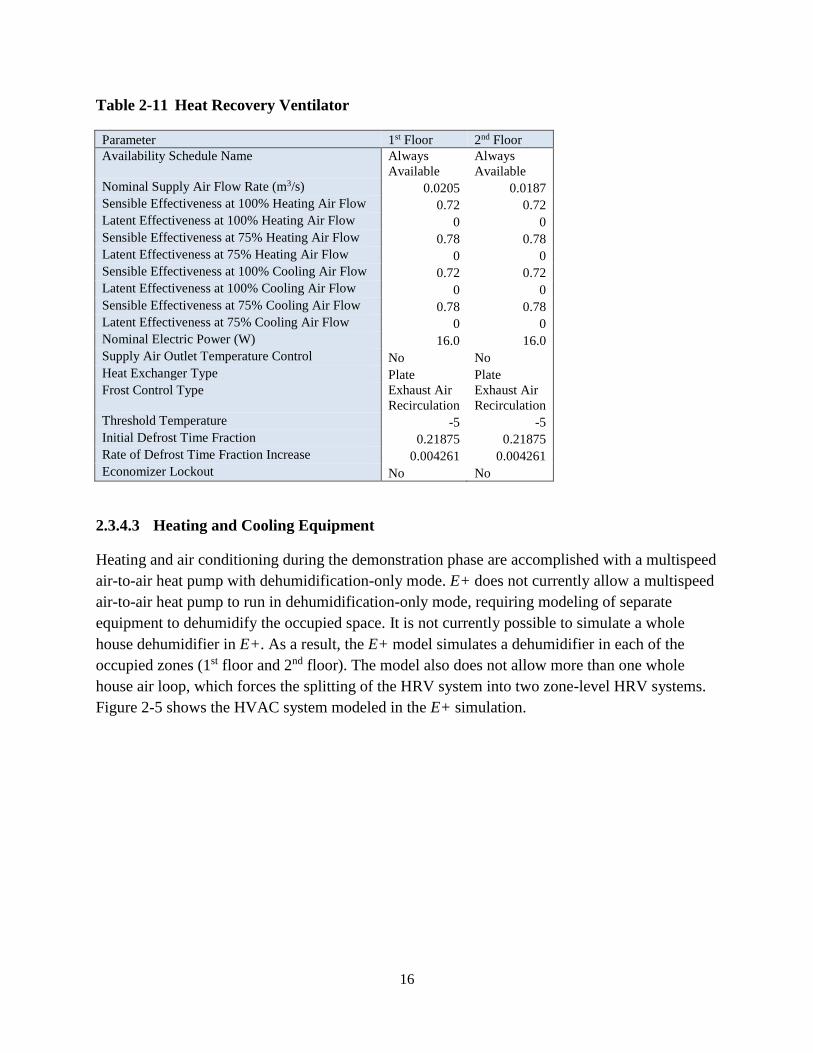
Table 2-11 Heat Recovery Ventilator

Parameter 1st Floor 2nd Floor

Availability Schedule Name Always

Available

Always

Available

Nominal Supply Air Flow Rate (m3/s) 0.0205 0.0187

Sensible Effectiveness at 100% Heating Air Flow 0.72 0.72

Latent Effectiveness at 100% Heating Air Flow 0 0

Sensible Effectiveness at 75% Heating Air Flow 0.78 0.78

Latent Effectiveness at 75% Heating Air Flow 0 0

Sensible Effectiveness at 100% Cooling Air Flow 0.72 0.72

Latent Effectiveness at 100% Cooling Air Flow 0 0

Sensible Effectiveness at 75% Cooling Air Flow 0.78 0.78

Latent Effectiveness at 75% Cooling Air Flow 0 0

Nominal Electric Power (W) 16.0 16.0

Supply Air Outlet Temperature Control No No

Heat Exchanger Type Plate Plate

Frost Control Type Exhaust Air

Recirculation

Exhaust Air

Recirculation

Threshold Temperature -5 -5

Initial Defrost Time Fraction 0.21875 0.21875

Rate of Defrost Time Fraction Increase 0.004261 0.004261

Economizer Lockout No No

2.3.4.3 Heating and Cooling Equipment

Heating and air conditioning during the demonstration phase are accomplished with a multispeed

air-to-air heat pump with dehumidification-only mode. E+ does not currently allow a multispeed

air-to-air heat pump to run in dehumidification-only mode, requiring modeling of separate

equipment to dehumidify the occupied space. It is not currently possible to simulate a whole

house dehumidifier in E+. As a result, the E+ model simulates a dehumidifier in each of the

occupied zones (1st floor and 2nd floor). The model also does not allow more than one whole

house air loop, which forces the splitting of the HRV system into two zone-level HRV systems.

Figure 2-5 shows the HVAC system modeled in the E+ simulation.

17

Figure 2-5 HVAC System Layout

The HVAC air-to-air heat pump is properly sized based on the assumed design day conditions

(i.e., oversized by 0 %). There are only 2 zones that require their temperature to be controlled by

the HVAC equipment, the 1st floor and 2nd floor. The 1st floor is used as the controlling zone, or

the location of the thermostat. This location will result in a floating of the 2nd floor air

temperatures. The basement is conditioned, but since the space is not finished and will not be

occupied during the demonstration phase, it is not necessary for the setpoint temperatures to be

met in the basement. The open web joist space and attic space are in the conditioned space, but

there is supply air from ductwork entering those spaces and the temperatures are allowed to fully

float.

The E+ input list in Table 2-12 are made for the sizing of thermal loads for each conditioned

zone. Note that there is no outdoor air drawn through the heating and cooling system ductwork.

All mechanical ventilation of outdoor air is supplied by the HRVs.

Table 2-12 Zone Sizing Parameters

Parameter Units 1st Floor 2nd Floor Basement

Zone Cooling Design Supply Air Temperature °C (°F) 12 (54) 12 (54) 12 (54)

Zone Heating Design Supply Air Temperature °C (°F) 30 (86) 30 (86) 30 (86)

Zone Cooling Design Supply Air Humidity kg-H2O/kg-air 0.008 0.008 0.008

Zone Heating Design Supply Air Humidity kg-H2O/kg-air 0.008 0.008 0.008

Outdoor Air Method Flow/Zone Flow/Zone Flow/Zone

Outdoor Air Flow Per Zone m3/s 0.0 0.0 0.0

Cooling Design Air Flow Method Design Day Design Day Design Day

Heating Design Air Flow Method Design Day Design Day Design Day

HRV 1

1st Floor (Control Zone)

2nd Floor

Dehumidifier

Dehumidifier

Building Envelope

Cool

Heat Supp. Heat

Fan HRV 2

18

The E+ input list in Table 2-13 is for the sizing of the air-to-air heat pump, which includes the

fan and coils. The outdoor air flow rate is autosized as the sum of the zone-specific outdoor air

flow rates, which totals to zero because the HRV system will meet all outdoor air requirements.

Table 2-13 HVAC System Sizing Parameters

Field Units Value

Type of Load to Size On Sensible

Design Outdoor Air Flow Rate m3/s Autosize

Minimum System Air Flow Ratio 0.40

Preheat Design Temperature °C (°F) 7 (45)

Preheat Design Humidity Ratio kg-H2O/kg-air 0.008

Precool Design Temperature °C (°F) 25 (77)

Precool Design Humidity Ratio kg-H2O/kg-air 0.008

Central Cooling Design Supply Air Temperature °C (°F) 12 (54)

Central Heating Design Supply Air Temperature °C (°F) 30 (86)

Sizing Option Non-Coincident

100 % Outdoor Air in Cooling No

100 % Outdoor Air in Heating No

Central Cooling Design Supply Air Humidity Ratio kg-H2O/kg-air 0.008

Central Heating Design Supply Air Humidity Ratio kg-H2O/kg-air 0.008

Cooling Design Air Flow Method Design Day

Heating Design Air Flow Method Design Day

The HVAC fan is a constant volume draw-through fan and has the E+ inputs listed in Table 2-14.

Table 2-14 HVAC Fan Parameters

Availability Always Available

Fan Efficiency 70 %

Pressure Rise 125 Pa

Maximum Flow Rate 0.42 m3/s

Motor Efficiency 90 %

Motor in Airstream Fraction 1.0

The NZERTF has a 2-ton AAON heat pump that has 2 speeds with gas reheat for

dehumidification control. The following tables define the parameters for a the 2-ton, 2-speed

heat pump based on Electrical Testing Labs (ETL) test data.

Table 2-15 shows the E+ inputs for the cooling coil, which is a multispeed air-cooled electric

direct expansion (DX) coil. The cooling coil is assumed to have two speeds, referred to as “low

19

speed” and “high speed.” At low speed, the coil capacity is 5483 W with a rated coefficient of

performance (COP) of 3.73 and a rated air flow rate of 0.23 m3/s (487 CFM). At high speed, the

coil capacity is 7751 W with a rated COP of 3.69 and a rated air flow rate of 0.42 m3/s

(890 CFM).

Table 2-15 Cooling Coil

Field Units Values


Condenser Type Air Cooled

Apply Part Load Fraction to Speeds Greater than 1 No

Apply Latent Degradation to Speeds Greater than 1 No

Fuel Type Electricity

Number of Speeds 2

Speed 1 Rated Total Cooling Capacity W 5483

Speed 1 Rated Sensible Heat Ratio 0.7

Speed 1 Rated COP 3.73

Speed 1 Rated Air Flow Rate m3/s 0.23

Speed 1 Rated Waste Heat Fraction of Power Input 0.1

Speed 1 Evaporative Condenser Effectiveness 0.9

Speed 2 Rated Total Cooling Capacity W 7751

Speed 2 Rated Sensible Heat Ratio 0.7




Speed 2 Evaporative Condenser Effectiveness 0.9

The cooling coil performance curve types can be found in Table 2-16. The specifics of each

curve are not reported here because of their complexity. Details on the functions are available

upon request.

Table 2-16 Cooling Coil Performance Curves

Cooling Coil Performance Curve Type Name Form

Total Cooling Capacity Function of Temp. Curve Heat Pump Cool Coil Cap-FT Biquadratic

Total Cooling Capacity Function of Flow Fraction Curve Heat Pump Cool Coil Cap-FF Quadratic

Energy Input Ratio Function of Temp. Curve Heat Pump Cool Coil EIR-FT Biquadratic

Energy Input Ratio Function of Flow Fraction Curve Heat Pump Cool Coil EIR-FF Quadratic

Part Load Fraction Correlation Curve Heat Pump Cool Coil PLF Quadratic

Waste Heat Function of Temperature Curve Waste Heat-FT Biquadratic

The heating coil E+ inputs can be found in Table 2-17. The heating coil is a multispeed electric

DX coil, and as with the cooling coil, the heating coil is assumed to have two speeds, referred to

20

as “low speed” and “high speed.” At low speed, the coil capacity is 4908 W with a rated COP of

4.02 and a rated air flow rate of 0.21 m3/s (487 CFM). At high speed, the coil capacity is 7675 W

with a rated COP of 4.19 and a rated air flow rate of 0.42 m3/s (890 CFM).

Table 2-17 Heating Coil

Field Units Value


Minimum ODB Temp. for Compressor Operation °C -17

Crankcase Heater Capacity W 0

Maximum ODB Temp. for Crankcase Heater Operation °C 10

Maximum ODB Temp. for Defrost Operation °C 7.22

Defrost Strategy Reverse Cycle

Defrost Control On Demand

Defrost Time Period Fraction 0.058333

Resistive Defrost Heater Capacity W Autosize

Apply Part Load Fraction to Speeds Greater than 1 No

Fuel Type Electricity

Number of Speeds 2

Speed 1 Rated Total Heating Capacity W 4908




Speed 2 Rated Total Heating Capacity W 7675




Note: ODB = Outdoor Dry-Bulb

The heating coil performance curve types can be found in Table 2-18. The specifics of each

curve are not reported here because of their complexity. Function details are available upon

request.

Table 2-18 Heating Coil Performance Curves

Heating Coil Performance Curve Category Name Form

Total Heating Capacity Function of Temp. Curve Heat Pump Heat Coil Cap-FT Cubic

Total Heating Capacity Function of Flow Fraction Curve Heat Pump Heat Coil Cap-FF Cubic

Energy Input Ratio Function of Temp. Curve Heat Pump Heat Coil EIR-FT Cubic

Energy Input Ratio Function of Flow Fraction Curve Heat Pump Heat Coil EIR-FF Quadratic

Part Load Fraction Correlation Curve Heat Pump Heat Coil PLF Quadratic

Waste Heat Function of Temperature Curve Waste Heat-FT Biquadratic

Defrost Energy Input Ratio Function of Temp. Curve Heat Pump Heat Coil DefCap-FT Biquadratic

21

The supplemental heating coil is an electric resistance heating element with an efficiency of 1.0

and an autosized capacity. The operation of the NZERTF will attempt to minimize the need for

the supplemental heating element.

The “tight” building envelope design could lead to high humidity issues throughout the year. The

advanced technology heat pump being installed in the NZERTF has the capability to run in

dehumidification-only mode. However, E+ cannot currently model such advanced equipment

and can only model dehumidifiers for a single zone. To overcome this limitation, the model

instead assumes operation of two dehumidifiers, one dedicated to each of the two occupied

floors. Since the building specifications include an Ultra-Aire 70H whole house ventilating

dehumidifier that was not actually used during the first year of operation, the simulations use

characteristics of that unit. The humidity level in the simulation model is controlled by two DX

dehumidifiers, one for each floor.

The dehumidifiers are operated based on the dehumidifying setpoint of 60 % (Hendron and

Engebrecht 2010). The equipment is available year-round to run whenever the relative humidity

reaches 60 % in its zone (1st floor or 2nd floor) regardless of whether the heat pump is running to

meet the setpoint temperature and when the heat pump is not running when the setpoint

temperature is met.

The specifications for this dehumidifier along with estimated water removal and energy factor

curves from the Ultra-Aire 70H are used to define the parameters and performance curves shown

in Table 2-19 and Table 2-20, which are used for the DX humidifiers in the simulation

(Christensen and Winkler 2009; Ultra-Aire 2011). The rated energy factor is assumed to be half

(1.0 L (0.26 gal.) per kWh) of the Ultra-Aire equipment rating (2.0 L (0.53 gal.) per kWh) to

ensure a conservative (high) electricity consumption estimate. The water removal rate of 30.75 L

(8.1 gal.) per day for the Ultra-Aire 70H is split between the 1st floor (16.08 L [4.24 gal.] per

day) and 2nd floor (14.67 L [3.86 gal.] per day) based on occupied volume. The model assumes

100 % of compressor heat is rejected into the conditioned zone. The Ultra-Aire 70H

dehumidifier will be located in the basement, causing the simulation model to slightly

overestimate the temperature level in each occupied zone.

Table 2-19 Dehumidifier Parameters

Field Units 1st Floor 2nd Floor

Availability Always Available Always Available

Rated Water Removal L/day (pints/day) 16.08 (33.98) 14.67 (31.00)

Rated Energy Factor L/kWh 1.0 1.0

Rate Air Flow Rate m3/s (CFM) 0.897 (190) 0.897 (190)

Min. Dry-Bulb °C (°F) -1.1 (30.0) -1.1 (30.0)

Max. Dry-Bulb °C (°F) 32.2 (90.0) 32.2 (90.0)

Off-Cycle Parasitic Elect. Load W 0.0 0.0

22

The dehumidifier water removal curve and energy factor curve coefficient values are shown in

Table 2-20.

Table 2-20 Dehumidifier Performance Curves

Curves Water Removal Energy Factor

Constant -1.281357458 -2.743752887

X 0.032064893 0.114491512

X2 -0.000280794 -0.001456831

Y 0.028356002 0.053860412

Y2 -0.000134939 -0.000244965

X*Y 0.000271496 -0.000362021

Min. X 4.4 4.4

Max. X 50 50

Min. Y 0 0

Max. Y 100 100

X= Inlet Air Dry-Bulb Temperature

Y= Inlet Air Relative Humidity

2.3.5 Domestic Hot Water

The domestic hot water (DHW) system installed in the NZERTF includes a number of potential

combinations of equipment, including 4 solar thermal collectors, two storage tanks, a heat

exchanger, and a heat pump water heater. The remainder of this section will define the DHW

system and the DHW consumption simulated during the demonstration phase of the NZERTF.

2.3.5.1 Domestic Hot Water Heater Equipment

The DHW system simulated in the model, as shown in Figure 2-6, is a two tank system located

in the basement with two solar thermal panels located on the east half of the front porch heating a

storage tank and an air-to-water heat pump downstream of the storage tank. The solar thermal

system uses a 50/50 water/glycol mix and indirectly heats the water in the storage tank through a

heat exchanger. The heat pump draws water from the storage tank and will further heat the water

if necessary to meet the target exit temperature of 48.9 °C (120 °F) for hot water use.

23

Figure 2-6 Domestic Hot Water Heating System

There are two tanks in the system, a 0.30 m3 (80 gal.) storage tank pre-heated by the solar

thermal system and a 0.19 m3 (50 gal.) tank connected to the heat pump. The maximum

temperature allowed is 76.6 °C (170.0 °F) for the storage tank and 71.1 °C (160.0 °F) for the

water heater tank. The heat pump turns on when the water heater tank water temperature drops

below 49.0 °C (120.2 °F) and turns off once the temperature increases to 54.0 °C (129.2 °F). The

back-up supplemental electric heating coil will turn on if the heat pump cannot maintain the

water temperature above 48.9 °C (120.2 °F) at the location in the tank of the electric coil. Based

on the heat pump characteristics and the location, the back-up electric heater should rarely be

required to meet the hot water demand. The Heliodyne HPAK heat exchanger is able to transfer

80 % of the energy from the solar thermal closed-loop system (Heliodyne 2012a).

The solar thermal collectors are Heliodyne GOBI 406 001 flat plate collectors with the

performance characteristics provided in Table 2-21 (Heliodyne 2012b). The maximum flow rate

is assumed to be the test flow rate.

Water

Heater

Tank

Storage Tank

Water Main

Heat

Exchang

er

DHW

End Uses

Tempering

Valve

Solar Collectors

Heat Pump

24

Table 2-21 Solar Thermal Collector Parameters

Field Units Value

Gross Area m2 2.503

Test Fluid Water

Test Flow Rate m3/s 0.0000498

Test Correlation Type Inlet

Efficiency Equation Coefficient 1 0.732

Efficiency Equation Coefficient 2 W/m2-K -4.195

Efficiency Equation Coefficient 3 W/m2-K2 0

Incident Angle Modifier Coefficient 2 0.0581

Incident Angle Modifier Coefficient 2 -0.2744

Max Flow Rate m3/s 0.0000498

The solar thermal loop pump operation control is based on 4 conditions. In order to ensure the

temperature in solar loop system does not get too high, the solar collector loop pump has a safety

mechanism that turns the pump on when the temperature of the gycol/water mix leaving the solar

collectors reaches 100 °C (212 °F). The solar collector loop pump is turned off when the

temperature in the water heater reaches 80 °C (176 °F). The solar collector loop pump is turned

on whenever the temperature of the fluid in the solar collector loop is 10 °C (18 °F) greater than

the water in the storage tank. The solar collector loop pump is turned off when the temperature of

the fluid in the solar collector loop is less than 2 °C (3.6 °F) higher than the water in the storage

tank.

Two plant loops are required in the simulation: the solar collector loop and domestic hot water

loop. The solar collector loop has a maximum temperature in the loop of 163 °C (325.4 °F) and a

minimum temperature of -45.6 °C (-50.1 °F). The domestic hot water loop has a maximum

temperature in the loop of 100 °C (212 °F) and a minimum temperature of 3.0 °C (37.4 °F). The

maximum flow rate for each plant loop is autosized while the minimum loop flow rate is 0.0 m3/s

(0.0 gpm). The loop is designed for an exit temperature – the temperature supplied to the “use

side” – of 48.9 °C (120.0 °F) for the domestic hot water loop and 100 °C (212 °F) for the solar

collector loop. For the solar collector loop, the exit temperature of the water is measured at the

point it enters the storage tank. For the domestic hot water loop, it is the temperature of the water

that is exiting the heat pump.

The storage tank and the water heater tank are both stratified tanks with 6 nodes. Their parameter

values are listed in Table 2-22. The storage tank inlet and outlet for the solar collector loop are

assumed to be at the lowest and highest node height, respectively. The water heater tank

parameters are based on the specifications for the initial equipment selected for installation into

the NZERTF.

25

Table 2-22 Storage Tank and Water Heater Tank Parameters

Field Units Storage Tank Hot Water

Heater Tank Tank Volume m3 0.303 0.189

Tank Height m 1.594 1.14

Tank Shape Vertical Cylinder Vertical Cylinder

Max. Temp. Limit °C 76.6 71.1

Heater 1 Setpoint Temperature °C 48.9

Heater 1 Deadband Temperature Difference Δ°C 5.0

Heater 1 Maximum Capacity W 3800

Heater 1 Height m 0.86

Heater 2 Setpoint Temperature °C 48.9

Heater 2 Deadband Temperature Difference Δ°C 10.0

Heater 2 Maximum Capacity W 3800

Heater 2 Height m 0.5

Ambient Temperature Indicator Zone Zone

Ambient Temperature Zone Name Basement Basement

Uniform Skin Loss Coefficient to Ambient Temperature W/m2·K 0.846 0.41

Skin Loss Fraction to Zone 1.0 1.0

Off Cycle Flue Loss Coefficient to Ambient Temperature W/K 0.0 0.0

Off Cycle Flue Loss Fraction to Zone 1.0 1.0

Use Side Effectiveness 1.0 1.0

Use Side Inlet Height m 0.398 0.229

Use Side Outlet Height m 1.46 1.09

Source Side Effectiveness 0.80 1.0

Source Side Inlet Height m 1.14 0.229

Source Side Outlet Height m 0.398 0.229

Inlet Mode Fixed Fixed

Use Side Design Flow Rate m3/s Autosize Autosize

Source Side Design Flow Rate m3/s Autosize Autosize

Indirect Water Heating Recovery Time h 1.5 1.5

Number of Nodes 6 6

The air-to-water heat pump is a Hubbell PBX 50-SL. The operation and performance parameter

values area listed in Table 2-23 and Table 2-24, respectively (Hubbell 2011). The heat pump

operation is based on the water temperature at the height of the second electric heating element

(0.5 m).

26

Table 2-23 Heat Pump Water Heater Operational Parameters

Field Units Value

Dead band Temperature Difference Δ°C 5.0

Compressor Setpoint Temperature °C 53.9

Condenser Water Flow Rate m3/s Autocalculate

Evaporator Air Flow Rate m3/s Autocalculate

Inlet Air Configuration Zone Air Only

Inlet Air Zone Name Basement

Min. Inlet Air Temp. for Compressor Operation °C 5

Compressor Location Basement

Parasitic Heat Rejection Basement

Fan Placement Draw Through

Temperature Control Sensor Location Heater 2

The heating coil for the air-to-water heat pump has a rated heating capacity of 1375 W and a

COP of 2.6. A factor not accounted for in the simulation model is that the heat pump will slightly

dehumidify the basement while operating.

Table 2-24 Hot Water Heat Pump Coil Parameters

Field Units Value

Rated Capacity W 1375

Rated COP W/W 2.6

Rated Sensible Heat Ratio 0.85

Rated Evaporator Inlet Air DB Temp. °C 19.7

Rated Evaporator Inlet Air WB Temp. °C 13.5

Rated Condenser Inlet Water Temp. °C 57.5

Rated Evaporator Air Flow Rate Autocalculate

Rated Condenser Air Flow Rate Autocalculate

Evaporator Fan Power Included in Rated COP Yes

Condenser Pump Power Included in Rated COP No

Condenser Pump Heat Included in Heat Cap. And COP No

Condenser Water Pump Power W 0

Fraction of Condenser Pump Heat to Water 0.2

The heat pump water heater fan and DHW fan parameter values are listed in Table 2-25.

27

Table 2-25 Heat Pump Water Heater Fan and DHW Fan Parameters

Field Fans


Fan Efficiency 80 %

Pressure Rise 100 Pa

Maximum Flow Rate Autosize

Motor Efficiency 90 %

Motor in Airstream Fraction 1.0

There are two intermittent pumps used in the DHW system, one for the solar thermal collectors

and one for the DHW loop. The parameter values for both pumps are shown in Table 2-26.

Table 2-26 Domestic Hot Water Loop Pump Parameters

Field Units DHW

Loop Pump

Solar Collector

Loop Pump Rate Flow Rate m3/s autosize 0.0000997

Rated Pump Head Pa 15 000 15 000

Rated Power Consumption W Autosize Autosize

Motor Efficiency 0.87 0.87

Fraction of Motor Inefficiency to Fluid Stream 0 0

Part Load Perf. Curve – Coefficient 1 0 0




Minimum Flow Rate m3/s 0 0

Pump control Type Intermittent Intermittent

2.3.5.2 Domestic Hot Water End Use

The DHW end use in the NZERTF has 5 categories: bath, shower, sinks, dishwasher, and clothes

washer. The use schedules in terms of fraction of peak flow (FPF) are shown in Figure 2-7, and

are based on Omar and Bushby (2013). The clothes washer is used 5 times a week: one load on

Wednesday and two loads on both Saturday and Sunday. The dishwasher is used for one load

five days a week: Monday, Wednesday, Friday, Saturday, and Sunday. The sink, shower, and

bath water draws vary by the occupancy schedule to match the target water use from Hendron

and Engebrecht (2010).

28

Figure 2-7 Domestic Hot Water End Use Schedules – Fraction of Peak Flow

0.0

0.5

1.0

0:0

01

:00

2:0

03

:00

4:0

05

:00

6:0

07

:00

8:0

09

:00

10

:00

11

:00

12

:00

13

:00

14

:00

15

:00

16

:00

17

:00

18

:00

19

:00

20

:00

21

:00

22

:00

23

:00

FPF

Shower and BathShower(Mon./Wed./Fri.)

Shower (Tues./Thurs.)

Shower (Sat.)

Shower (Sun.)

Bath (Mon.-Tues./Thurs./Fri./Sun.)

Bath (Wed.)

Bath (Sat.)

0.0

0.5

1.0

0:0

0

1:1

5

2:3

0

3:4

5

5:0

0

6:1

5

7:3

0

8:4

5

10

:00

11

:15

12

:30

13

:45

15

:00

16

:15

17

:30

18

:45

20

:00

21

:15

22

:30

23

:45

FPF

Sinks Kitchen Sink (Mon.)

Kitchen Sink (Tues./Thurs.)

Kitchen Sink (Wed.)

Kitchen Sink (Fri.)

Kitchen Sink (Sat.)

Kitchen Sink (Sun.)

Master Sink (Mon.)

Master Sink (Tues./Thurs.)

Master Sink (Wed.)

Master Sink (Fri.)

Master Sink (Sat.)

Master Sink (Sun.)

0

0.5

1

0:0

0

1:1

5

2:3

0

3:4

5

5:0

0

6:1

5

7:3

0

8:4

5

10

:00

11

:15

12

:30

13

:45

15

:00

16

:15

17

:30

18

:45

20

:00

21

:15

22

:30

23

:45

FPF

Cothes Washer and DishwasherDishwasher (Tues./Thurs.)

Dishwasher(Mon./Wed./Fri./Sun.)Dishwasher (Tues./Thurs.)

Dishwasher (Sat.)

Clothes Washer (Mon-Tues.,Thurs.-Fri.)Clothes Washer (Wed.)

29

Table 2-27 defines DHW use in terms of daily water use, water temperature, and heat gain

fractions (fraction of energy in water that is released to the ambient environment). Hendron and

Engebrecht (2010) is used to calculate daily water consumption and heat gains for each of the

categories except for the dishwasher and clothes washer, which are based on Omar and Bushby

(2013) and the equipment’s Energy Star ratings.

Table 2-27 Domestic Hot Water Use and Thermal Load Fractions

DHW Use

Category

Water Temp.

°C (°F)

Daily

L (Gal)

Sensible Load

Fraction

Latent Load

Fraction

Clothes Washer 48.9 (120.0) 35.7 (9.43) 0.0 0.0

Dishwasher 48.9 (120.0) 4.2 (1.12) 0.0 0.0

Shower 40.6 (105.0) 142.4 (37.6) 0.2127 0.005655

Bath 40.6 (105.0) 11.3 (3.0) 0.2083 0.0

Sinks 40.6 (105.0) 93.6 (24.7) 0.09869 0.00127

The sink, shower, and bath water draws are assumed to be mixed water use at 40.6 °C (105.1 °F).

The sink flow rates are 5.7 L (1.5 gal.) per min while the shower and bath flow rates are 6.6 L

(1.75 gal.) per min. The sensible and latent load fractions for the sink, shower, and bath draws

are calculated by reverse engineering using the heat gain estimate equations in Hendron and

Engebrecht (2010). Omar and Bushby (2013) defines sink draws in 21 second intervals while the

E+ model can only model at one minute increments. The consolidation of draws results in the

total length of draws for a week being 6 seconds longer than stated in Omar and Bushby (2013),

or additional hot water use of 29.5 L (7.8 gal.). The additional DHW use will slightly

overestimate electricity use relative to that provided by Omar and Bushby (2013).

The domestic hot water use equipment is assumed to use water at the exit target temperature of

the water heater and has no sensible or latent heat gains resulting from the hot water use. The

clothes washer is assumed to consume 46.4 L (12.25 gal.) per cycle. Total water use is the

product of the water use per cycle and the number of loads per year (260) for a total of 12 057 L

(3185 gal.) per year or 33.0 L (8.73 gal.) per day. The dishwasher is assumed to consume 5.9 L

(1.57 gal.) per cycle. Similar to the clothes washer, total water use is the product of the water use

per cycle and the number of loads per year (260) for a total of 1545 L (408 gal.) per year or 4.24

L (1.12 gal.) per day.

2.3.6 Solar Photovoltaic

Energy efficient design reduces but does not eliminate electricity use by the NZERTF. Solar

photovoltaic (PV) panels are installed on the roof of the NZERTF to produce at least as much

electricity as is consumed by the NZERTF on an annual basis.

Figure 2-3 shows that there are 32 SunPower SPR-320E-WHT-U solar PV panels installed on

the roof of the NZERTF in 4 horizontal rows of 8 panels each. Two rows are connected to two

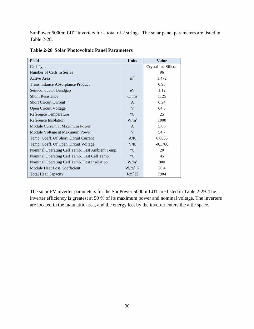
30

SunPower 5000m LUT inverters for a total of 2 strings. The solar panel parameters are listed in

Table 2-28.

Table 2-28 Solar Photovoltaic Panel Parameters

Field Units Value

Cell Type Crystalline Silicon

Number of Cells in Series 96

Active Area m2 1.472

Transmittance Absorptance Product 0.95

Semiconductor Bandgap eV 1.12

Shunt Resistance Ohms 1125

Short Circuit Current A 6.24

Open Circuit Voltage V 64.8

Reference Temperature °C 25

Reference Insolation W/m2 1000

Module Current at Maximum Power A 5.86

Module Voltage at Maximum Power V 54.7

Temp. Coeff. Of Short Circuit Current A/K 0.0035

Temp. Coeff. Of Open Circuit Voltage V/K -0.1766

Nominal Operating Cell Temp. Test Ambient Temp. °C 20

Nominal Operating Cell Temp. Test Cell Temp. °C 45

Nominal Operating Cell Temp. Test Insolation W/m2 800

Module Heat Loss Coefficient W/m2·K 30.4

Total Heat Capacity J/m2·K 7984

The solar PV inverter parameters for the SunPower 5000m LUT are listed in Table 2-29. The

inverter efficiency is greatest at 50 % of its maximum power and nominal voltage. The inverters

are located in the main attic area, and the energy lost by the inverter enters the attic space.

31

Table 2-29 Solar Photovoltaic Inverter Parameters

Field Units Value

Availability Schedule Name Always Available

Zone Name Main Attic (Zone 4)

Radiative Fraction 0.05

Rated Maximum Continuous Output Power W 5000

Night Tare Loss Power W 0.1

Nominal Voltage Input V 438

Eff. At 10 % Power and Nominal Voltage 0.935






33

3 Pre-Demonstration Phase Model Results

This section will summarize the results from the pre-demonstration phase simulation results and

compare those to the measured consumption during the demonstration phase.

3.1 Total Electricity Consumption and Production

The pre-demonstration phase simulation estimates total electricity consumption of the NZERTF

to be 11 156 kWh and total electricity production to be 14 222 kWh (see Figure 3-1). The

measured consumption is 16 % higher (12 927 kWh) and measured production is 5 % lower

(13 523 kWh) than the simulated results. The NZERTF reached its net-zero energy goal, but the

excess production was lower than was forecasted by the model by 2471 kWh.

Figure 3-1 Annual Electricity Consumption and Production (kWh)

Electricity consumption by category for the simulation and measured performance is shown in

Figure 3-2. The simulation overestimates consumption for three categories (Miscellaneous

Electrical Loads - MELs - and appliances, lighting, and HRV) and underestimates consumption

for three categories (heating and cooling, DHW, and solar loop pumps).8 The ranking of the

magnitude differences (greatest to smallest) is as follows: heating and cooling (-1960 kWh), plug

loads/appliances (+718 kWh), DHW (-484 kWh), solar loop pumps (-243 kWh), lighting

(+217 kWh), and the HRV (+44 kWh).

8 The simulation estimates consumption by the solar PV inverters to be 3 kWh annually. The measured performance

data does not include such a category. Therefore, it is excluded from this discussion.

11 156

12 92714 222

13 523

0

2 000

4 000

6 000

8 000

10 000

12 000

14 000

16 000

AMY Actual

Pre-Demonstration Phase Measured

kW

h

Total Energy

Consumption

Total Energy

Production

34

Figure 3-2 Total Electricity Consumption by Category - kWh

3.2 MELs, Appliances, and Lighting

Figure 3-3 shows the annual electricity consumption for all MELs and appliances. For

appliances, the most significant difference in consumption occurs for the clothes dryer, which is

overestimated in the simulation by 819 kWh (151 %), followed by the dishwasher (187 kWh or

194 %). The simulation model underestimates consumption for the refrigerator, oven, and

microwave (74 kWh, 71 kWh, and 58 kWh, respectively) while consumption is slightly

overestimated for the cooktop/range hood (11 kWh). The consumption by the MELs (a.k.a., plug

loads) is overestimated in four rooms (living room, office, master bedroom/bathroom, and 3rd

bedroom) and underestimated in three rooms (basement, kitchen, and 2nd bedroom). The most

significant overestimations occur for the living room MEL (324 kWh) and office MEL

consumption (52 kWh). These overestimations account for most of the MELs in the basement

(518 kWh) of the NZERTF, which are completely excluded from the simulation (see Figure 3-3).

Basement MELs are primarily standby loads that were shifted from the main floor (living room

and office) to the basement during the demonstration phase because the monitoring and control

equipment in the basement were already consuming significant standby wattage and creating the

associated heat loads.

4211

6171

558

514

653

435

5025

4307

628

1,112

75

318

0

1 000

2 000

3 000

4 000

5 000

6 000

7 000

8 000

9 000

10 000

11 000

12 000

13 000


kW

h

Solar Loop Pumps

DHW

MELs & Appliances

Lighting

HRV

Heating and Cooling

35

Figure 3-3 Appliances and Plug Loads (MELs) by Room – kWh

The annual lighting consumption in the simulation is 50 % higher than the measured

consumption. Figure 3-4 shows both the simulated and measured monthly electricity

consumption for lighting. Both the simulated and measured lighting electricity consumption is

relatively constant around 55 kWh and 36 kWh, respectively. The overestimation is relatively

constant, ranging between 40 % and 54 % (excluding August at 74 %).

Figure 3-4 Lighting by Room – kWh

0

200

400

600

800

1000

1200

1400

Bas

emen

t

Kit

chen

Liv

ing R

oo

m

Off

ice

Mas

ter

Bed

/Bat

h

2nd

Bed

room

3rd

Bed

room

Clo

thes

Was

her

Clo

thes

Dry

er

Ref

rig

erat

or

Coo

kto

p/H

oo

d

Ov

en

Mic

row

ave

Dis

hw

ash

er

MELs Appliances

kW

h Pre-

Demonstration

Phase

Measured

0

10

20

30

40

50

60

Ele

ctri

city

Con

sum

pti

on

(kW

h)

Pre-

Demonstration

Phase

Measured

36

The manner in which the simulation incorporates electrical equipment (plug loads and

appliances) and lighting is straightforward. For each item, E+ requires a peak wattage and load

schedule. In order to better represent the actual operation and measured consumption, both of

these factors must be considered to see where the discrepancy occurs and adjust the simulation to

match the actual activity and performance during the demonstration phase of the NZERTF.

Additionally, particular interest should be placed on the measured performance of the NZERTF

during the month of August.

3.3 HVAC, DHW, and Solar Systems

The complex systems (HVAC, DHW, solar thermal, and solar PV) in the NZERTF require

detailed analysis to determine where the discrepancies are occurring because a significant

number of assumptions must be defined and there may be interactions between systems.

3.3.1 HVAC Equipment

The heating and cooling equipment for the NZERTF includes the air-to-air heat pump with

dehumidify-only mode and auxiliary electric back-up unit. As discussed in Section 2.3.4, the

simulation includes zone dehumidifiers to incorporate dehumidify-only mode into the model.

Figure 3-5 shows the electricity consumption by month to meet the heating and cooling loads of

the NZERTF. The simulation results show comparable trends in the heating and cooling, but the

total monthly consumption is consistently lower than the measured consumption regardless of

season. The greatest differences occur during the coldest months of the demonstration phase

(December through March). All assumptions and parameters should be reviewed and compared

to measured performance data to determine how to better represent the installed equipment and

its performance.

Figure 3-5 Heating and Cooling Consumption by Month – kWh

0100200300400500600700800900

1000110012001300

kW

h

Measured -

Cooling

Pre-

Demonstration

Phase - Cooling

Measured -

Heating

Pre-

Demonstration

Phase - Heating

37

The HRV system in the NZERTF consumes electricity at a relatively constant rate (see Figure

3-6), with total electricity consumption varying by month due to the number of days in a month.

The simulation consistently consumes greater electricity than was measured during the

demonstration phase. The most apparent is the month of August, in which the measurements

show an anomalous dip below 40 kWh, and may be due to the lost data or equipment faults that

occurred during the demonstration phase. The assumed wattage and air flow rate for the HRV

should be reviewed to determine if the ventilation rate or wattage are set lower than was

measured in the NZERTF.

Figure 3-6 HRV Electricity Consumption by Month - kWh

3.3.2 DHW and Solar Thermal System

The DHW and solar thermal systems are integrated and require simultaneous consideration when

analyzing electricity consumption of both systems. The solar loop pumps in the simulation

consume only 24 % of the measured solar loop pump electricity consumption. Similarly, the

DHW system (heat pump water heater with electric auxiliary element) consumes only 56 % of

the measured heat pump electricity consumption. Although the consumption is much lower in the

pre-demonstration simulation, the general trends hold in Figure 3-7, with more DHW electricity

consumption and less solar collector loop operation during the colder months and vice versa

during the summer months. Parameter values and assumptions of the DHW and solar loop in the

simulation should be reviewed to determine what to change to better represent the measured

performance.

0

10

20

30

40

50

kW

h

Pre-

Demonstration

Phase

Measured

38

Figure 3-7 DHW and Solar Loop Pump Electricity Consumption by Month – kWh

Figure 3-8 shows that the average pre-heated storage tank and heat pump water heater tank

temperatures from the simulation results map well to the measured tank temperatures. It is

important to note that the measured tank temperatures are not internal measurements, but based

on the tank outlet water temperature. As a result, it is likely that the average temperature for the

entire tank would be lower than the temperature of the outlet water, which is drawn from the top

of the tank. The parameters and assumptions of the solar loop and pre-heated storage tank in the

simulation should be reviewed to determine what to change to better represent the measured

performance, with particular focus on the results for August to determine if the difference is due

to incorrect simulation assumptions or faults during operation.

0

20

40

60

80

100

120

140

160k

Wh

Pre-Demo Phase -

Water Heater

Pre-Demo Phase -

Solar Loop Pumps

Measured - Water

Heater

Measured - Solar

Loop Pumps

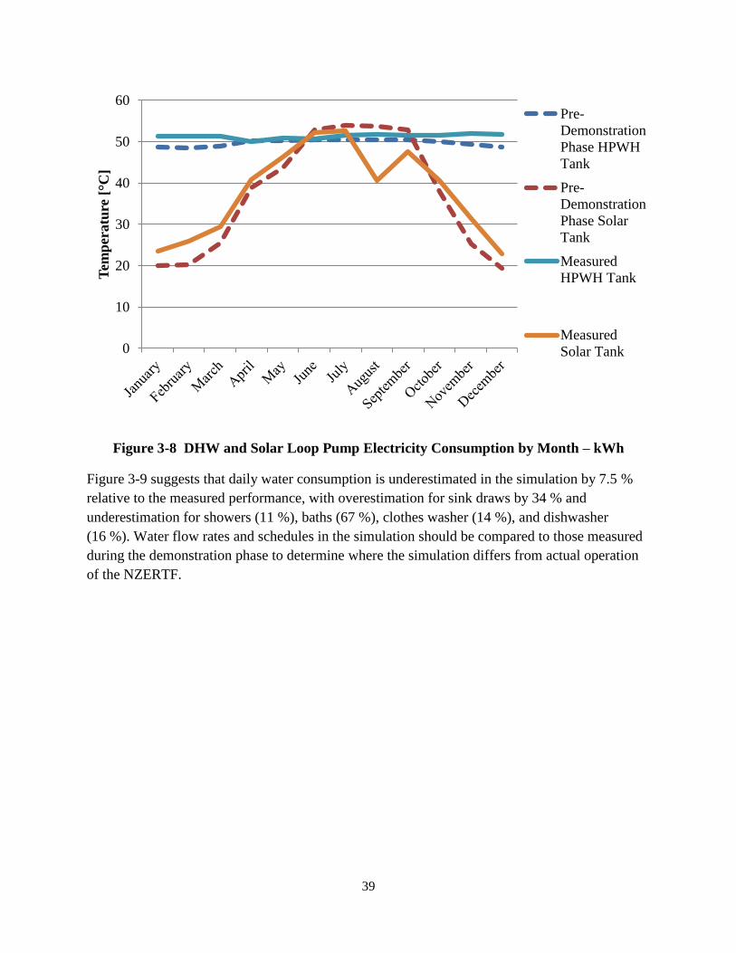
39

Figure 3-8 DHW and Solar Loop Pump Electricity Consumption by Month – kWh

Figure 3-9 suggests that daily water consumption is underestimated in the simulation by 7.5 %

relative to the measured performance, with overestimation for sink draws by 34 % and

underestimation for showers (11 %), baths (67 %), clothes washer (14 %), and dishwasher

(16 %). Water flow rates and schedules in the simulation should be compared to those measured

during the demonstration phase to determine where the simulation differs from actual operation

of the NZERTF.

0

10

20

30

40

50

60T

emp

eratu

re [°C

]Pre-

Demonstration

Phase HPWH

Tank

Pre-

Demonstration

Phase Solar

Tank

Measured

HPWH Tank

Measured

Solar Tank

40

Figure 3-9 Daily Water Consumption – Gallons9

Since the hot water demand will impact the loads on the heat pump water heater and solar

thermal system, it is possible that the underestimation of water consumption could lead to greater

electricity consumption by both the DHW system and solar thermal system.

3.3.3 Solar Photovoltaic Generation

The simulation overestimates annual electricity production by 5 % (698 kWh). Figure 3-10

shows that the simulation overestimates production for seven months and underestimates

production for the other five months. The biggest deviations are for August (384 kWh) followed

by July (184 kWh), which together account for 80 % of the overestimated production. The dip in

July and August should be analyzed in greater detail to determine whether the difference is a

result of faults in operation of the NZERTF or assumptions in the simulation.

9 1 gallon = 3.785 liters

37.642.4

3.0

9.0

25.2

18.8

10.5

12.31.1

1.3

0

5

10

15

20

25

30

35

40

45

50

55

60

65

70

75

80

85


Gall

on

s

Dishwasher

Clothes Washer

Sink

Baths

Showers

41

Figure 3-10 Total Electricity Consumption and Solar PV Production (kWh) - Monthly

0

200

400

600

800

1000

1200

1400

1600

1800k

Wh Measured

Pre-Demonstration

Phase

43

4 Adjustments to Simulation Model

Variations in energy consumption between the simulation and the measured performance are

most significant for the DHW system, HVAC system, and solar thermal system. Adjustments are

also made in the assumed infiltration rate, lighting, MEL loads, and appliance loads. There are

no changes considered to the other aspects of the building envelope because the specifications

are relatively straightforward to replicate in the simulation model.

4.1 Infiltration

The most recent air leakage test led to a higher infiltration rate of 0.223 m3/s (470 CFM) or 0.63

ACH50. The infiltration rate is converted to ELA, as is used in the pre-demonstration phase

simulation (see Section 2.1), using the following formula from Chapter 16 in ASHRAE (2012):

𝐴𝐿 = 10 000 ∗ 𝑄𝑟 ∗ √𝜌/2∆𝑝𝑟

𝐶𝐷

Where 𝐴𝐿 = 𝑒𝑞𝑢𝑖𝑣𝑎𝑙𝑒𝑛𝑡 𝑜𝑟 𝑒𝑓𝑓𝑒𝑐𝑡𝑖𝑣𝑒 𝑎𝑖𝑟 𝑙𝑒𝑎𝑘𝑎𝑔𝑒 𝑎𝑟𝑒𝑎 (𝑐𝑚2)

𝑄𝑟 = 𝑝𝑟𝑒𝑑𝑖𝑐𝑡𝑒𝑑 𝑎𝑖𝑟𝑓𝑙𝑜𝑤 𝑟𝑎𝑡𝑒 𝑎𝑡 ∆𝑝𝑟 (𝑚3 𝑠⁄ )

𝜌 = 𝑎𝑖𝑟 𝑑𝑒𝑛𝑠𝑖𝑡𝑦 (𝑘𝑔 𝑚3⁄ )

∆𝑝𝑟 = 𝑟𝑒𝑓𝑒𝑟𝑒𝑛𝑐𝑒 𝑝𝑟𝑒𝑠𝑠𝑢𝑟𝑒 𝑑𝑖𝑓𝑓𝑒𝑟𝑒𝑛𝑐𝑒 (𝑃𝑎)

𝐶𝐷 = 𝑑𝑖𝑠𝑐ℎ𝑎𝑟𝑔𝑒 𝑐𝑜𝑒𝑓𝑓𝑖𝑐𝑖𝑒𝑛𝑡

ASHRAE (2012) states that ELA at 4 Pa, as used in E+, typically assumes a discharge

coefficient (𝐶𝐷) of 1.0. The reference pressure difference (∆𝑝𝑟) used in the blower door test is

50 Pa. The air density (𝜌) is assumed to be 1.2922 𝑘𝑔 𝑚3⁄ . Filling in the equation leads to an

estimated ELA of 253.5 cm2, which is an increase of 64.5 cm2 (34 %) relative to the pre-

demonstration phase simulation infiltration rate. As in Kneifel (2013), the infiltration is split

between the 1st floor (132.6 cm2) and 2nd floor (120.9 cm2) based on total volume.

4.2 MELs and Appliances

The peak wattage parameter values used in the pre-demonstration phase simulation were based

on specification sheets for the initial appliances and electronics (MELs) selected for installation

in the NZERTF. However, some of the appliances installed in the NZERTF are different than

those initially selected due to complexities related to the product acquisitions process. The peak

wattage for each appliance is adjusted in the simulation, as shown in Table 4-1, based on updated

specification sheets for the equipment actually installed in the NZERTF, measured performance

data based on laboratory testing, or actual measured consumption during the demonstration

phase.

44

Table 4-1 Adjustments to Peak Wattage for Appliances and MELs

Appliance Pre-Demonstration Phase

Peak Wattage

Adjusted Peak

Wattage

Refrigerator 45.7 56

Clothes Washer 500 340

Clothes Dryer 5200 2411

Dishwasher 1090 346

Range – Oven 5100 5950

Range – Cooktop 3600* 3381

Range – Hood 330 75

Microwave 950 1618

*Assumes the use of only 2 burners.

Note: Peak wattage is set based on either the average wattage over a cycle of

operation or set to meet the target energy consumption for a given appliance.

4.3 Lighting

Figure 3-2 shows that the simulation over-consumes lighting-related electricity. After

investigating the lighting loads during the demonstration phase, it was determined that the

simulation assumed peak wattage to be higher than measured wattage during the demonstration

phase for nearly every room in the NZERTF. The values shown in Table 4-2 are the

pre-demonstration phase lighting wattages in the simulation and the actual wattages that were

determined experimentally by turning on the lights in each room and physically measuring the

actual wattage drawn. Total peak wattage (excluding the unused basement lighting) dropped

from 614 W to 408 W, which makes the pre-demonstration phase wattage 150 % of the post-

demonstration phase simulation values. Note that there is some uncertainty in the measured

wattage because there are some errors in the electrical system, where some light fixtures are

wired to a breaker that is inconsistent with the specifications (e.g., light in hallway may be wired

to a bedroom breaker). These inconsistencies do not have an impact on total electricity

consumption related to lighting, and negligible impacts on the associated heat loads.

45

Table 4-2 Adjustments to Lighting Peak Wattage by Room

Floor Room Pre-Demonstration

Phase

(Watts)

Post-Demonstration

Phase

(Watts)

1st Kitchen 118 81

Dining Room 65 34

Living Room 118 55

Office 0 0

1st Floor Bath 46 30

2nd Master Bedroom 41 41

2nd Bedroom 41 39

3rd Bedroom 41 33

Master Bathroom 81 82

2nd Bathroom 63 13

Basement* 217 217

*Never turned on

4.4 HVAC System

During the investigation of the measured performance of the HVAC system, many parameter

values for the components in the HVAC system (cooling coil, heating coils, dehumidifiers, and

HRV) should be adjusted in the pre-demonstration phase simulation to better represent the actual

performance of the equipment during the demonstration phase of the NZERTF. Parameter values

are based on the E+ rating conditions for each heating and cooling system component.

The cooling DX coil in the simulation represents the performance of the air-to-air heat pump in

cooling mode. The rated capacity, sensible heat ratio, COP, and air flow rate were adjusted for

both the low-speed and high-speed cooling operation mode of the heat pump (see Table 4-3).

The cooling COP and rated capacity values decrease, which will increase electricity consumption

required to meet the cooling load relative to the pre-demonstration phase simulation results.

Table 4-3 Changes in Cooling DX Coil Parameters

Field Units Values Adjusted Values

Availability Cooling Season Always Available

Speed 1 Rated Total Cooling Capacity W 5483 5182

Speed 1 Rated Sensible Heat Ratio 0.70 0.75

Speed 1 Rated COP 3.73 3.66

Speed 1 Rated Air Flow Rate m3/s 0.23 0.284

Speed 2 Rated Total Cooling Capacity W 7751 6889

Speed 2 Rated Sensible Heat Ratio 0.70 0.75



Crankcase Heater Capacity (Represents Standby W) W 0 50

46

The heating DX coil in the simulation represents the performance of the air-to-air heat pump in

heating mode. The rated capacity, COP, and air flow rate were adjusted for both the low-speed

and high-speed heating operation mode of the heat pump. As shown in Table 4-4, the air flow

rate and capacity for both low-speed and high-speed operation modes increase while the rated

COP for high-speed operation decreases. The measured COP of the heat pump is lower in

heating mode because the original rated values are based on standard test procedure conditions,

which do not account for the common occurrence of frost build-up in the refrigerant piping.

Measured data is used to estimate static-state performance values with frost build-up that better

represent “real world” operating conditions.10

The crankcase heater is added as a proxy to account for the standby electricity consumption of

the heat pump during the heating season, with capacity of 50 W and maximum temperature of

crankcase heater operation set at 100 °C (212 °F). The defrost parameter values were adjusted

based on actual equipment operation and experimental data collected during the demonstration

phase. Heating coil defrost occurs when the outdoor temperature is below 1.7 °C (35 °F), and is

accomplished by operating the 10 kW electric resistive auxiliary element approximately every 90

minutes. The median length of defrost cycle during the demonstration phase is 148 seconds,

ranging from 60 seconds to 552 seconds. Based on the median defrost cycle length during the

demonstration phase, the defrost time period fraction is 0.0273.

Table 4-4 Changes in Heating DX Coil Parameters

Field Units Value Adjusted Values

Crankcase Heater Capacity W 0 50

Maximum ODB Temp. for Crankcase Heater Operation °C 10 100

Maximum ODB Temp. for Defrost Operation °C 7.22 1.7

Defrost Strategy Reverse Cycle Resistive

Defrost Control On Demand Timed

Defrost Time Period Fraction 0.058333 0.0273

Resistive Defrost Heater Capacity W Autosize 10 000

Speed 1 Rated Total Heating Capacity W 4908 5159



Speed 2 Rated Total Heating Capacity W 7675 7545


Speed 2 Rated Air Flow Rate m3/s 0.42 Autosize

The efficiency of the auxiliary electric resistance heating coil is decreased from 1.00 to 0.98

because no electric resistance coil is 100 % efficient. The wattage of the auxiliary coil is changed

from “autosized” by the E+ software to 10 000 W to match the size of the actual heat pump

installed in the NZERTF. 10 Capacity and power curves based on measured data are available upon request.

47

The efficiency of the HRV in the pre-demonstration phase simulation is greater than the

measured performance of the HRV. Experimental data at or near the rated test conditions used in

E+ is used to adjust the parameter values to those shown in Table 4-5. The effectiveness is

reduced for all flow rates while the supply air flow rate (0.0392 m3/s (83 CFM) to 0.04956 m3/s

(105 CFM)) is increased to match measured performance. The electric power wattage is adjusted

based on the relative volume of the two floors.

Table 4-5 Changes in Heat Recovery Ventilator Parameters

Parameter

Pre-Demonstration Phase Adjusted

1st Floor 2nd Floor 1st Floor 2nd Floor

Nominal Supply Air Flow Rate (m3/s) 0.0205 0.0187 0.02592 0.02364

Sensible Effectiveness at 100% Heating Air Flow 0.72 0.72 0.62 0.62

Sensible Effectiveness at 75% Heating Air Flow 0.78 0.78 0.68 0.68

Sensible Effectiveness at 100% Cooling Air Flow 0.72 0.72 0.62 0.62

Sensible Effectiveness at 75% Cooling Air Flow 0.78 0.78 0.68 0.68

Nominal Electric Power 27.0 27.0 28.2 25.8

The dehumidification option on the air-to-air heat pump is simulated using zone dehumidifiers.

The humidistat in the pre-demonstration phase simulation of 60 % relative humidity is adjusted

to 50 %, which is the setpoint during the demonstration phase of the NZERTF. The

dehumidification equipment parameter values for water removal and energy factor in the pre-

demonstration phase simulation were expected to be conservative estimates when selected. These

parameters are adjusted as shown in Table 4-6 based on both the whole house dehumidifier’s

rated values and the measured performance of the dehumidify mode of the air-to-air heat pump.

Table 4-6 Changes in Dehumidifier Parameters

Field Units 1st Floor 2nd Floor

Rated Water Removal L/day (pints/day) 16.08 to 17.3 (34.0 to 36.6) 14.67 to 15.8 (31.0 to 33.4)

Rated Energy Factor L/kWh 1.00 to 1.65 1.00 to 1.65

4.5 DHW and Solar Thermal Systems

The DHW and solar thermal systems were dramatically under-consuming electricity in the

simulation results relative to measured consumption during the demonstration phase. All

assumptions and parameters in the simulation were reviewed, which led to a number of key

changes to the simulation, including system design, components, operation, and efficiency as

well as hot water demand. The key change to the system design is to make the solar collectors in

parallel as shown in Figure 4-1 instead of in series as shown in Figure 2-6.

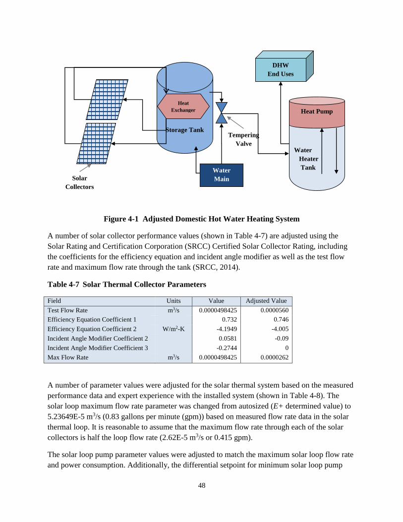
48

Figure 4-1 Adjusted Domestic Hot Water Heating System

A number of solar collector performance values (shown in Table 4-7) are adjusted using the

Solar Rating and Certification Corporation (SRCC) Certified Solar Collector Rating, including

the coefficients for the efficiency equation and incident angle modifier as well as the test flow

rate and maximum flow rate through the tank (SRCC, 2014).

Table 4-7 Solar Thermal Collector Parameters

Field Units Value Adjusted Value

Test Flow Rate m3/s 0.0000498425 0.0000560

Efficiency Equation Coefficient 1 0.732 0.746

Efficiency Equation Coefficient 2 W/m2-K -4.1949 -4.005

Incident Angle Modifier Coefficient 2 0.0581 -0.09

Incident Angle Modifier Coefficient 3 -0.2744 0

Max Flow Rate m3/s 0.0000498425 0.0000262

A number of parameter values were adjusted for the solar thermal system based on the measured

performance data and expert experience with the installed system (shown in Table 4-8). The

solar loop maximum flow rate parameter was changed from autosized (E+ determined value) to

5.23649E-5 m3/s (0.83 gallons per minute (gpm)) based on measured flow rate data in the solar

thermal loop. It is reasonable to assume that the maximum flow rate through each of the solar

collectors is half the loop flow rate (2.62E-5 m3/s or 0.415 gpm).

The solar loop pump parameter values were adjusted to match the maximum solar loop flow rate

and power consumption. Additionally, the differential setpoint for minimum solar loop pump

Water

Heater

Tank

Storage Tank

Water

Main

Heat

Exchanger

DHW

End Uses

Tempering

Valve

Solar

Collectors

Heat Pump

49

operation was changed from 2.0 °C (3.6 °F) to 3.0 °C (5.4 °F) to match the actual operation

conditions in the NZERTF.

Table 4-8 Solar Loop Pump Parameters

Field Units Pre-Demonstration

Phase Values

Adjusted Values

Rate Flow Rate m3/s 0.000099685 0.0000523649

Rated Pump Head Pa 15000 179352

Rated Power Consumption W Autosize 160

The pre-demonstration phase simulation excluded any heat losses through pipes (adiabatic)

running to and from the solar collectors and the solar loop tank, or from the solar loop tank to the

heat pump water heater tank. The adjusted model includes 6.1 m (20 ft) of outdoor pipe to and

from the solar collectors to the interior of the NZERTF, 15.24 m (50.0 ft) of indoor pipe running

to and from the outdoor pipe to the solar loop tank, and 3.2 m (10.5 ft) of pipe from the solar

loop tank to the heat pump water heater tank. All pipes (indoor and outdoor) are assumed to be

copper and rapped with RSI-0.7 (R-4) insulation.

Due to the complexity of the DHW system and solar thermal system, the model was simplified

by replacing the “stratified” water tanks (accounts for vertical stratification of water with the

hottest at the top) for both the solar loop tank and heat pump water heater tank with “mixed”

tanks (equal heat distribution throughout water). The 100 % mixing of the tanks makes the

temperature equal throughout the volume of water, leading to the location of inlet and outlets for

each tank unimportant to the model. Additionally, some of the parameter values were changed

(see Table 4-9) to better represent the performance of the installed tanks, including the maximum

temperature limits and loss coefficients to ambient temperature for both tanks, deadband

temperature difference and auxiliary electric heating element capacity for the heat pump water

heater tank, and source-side effectiveness for the solar loop tank.11

11 Note: The mixed tanks could be replaced with the stratified tanks to see if it changes the performance.

50

Table 4-9 Changes in Storage Tank and Hot Water Heater Tank Parameters

Field Units Storage Tank Water Heater Tank

Value Adjusted Value Value Adjusted Value

Tank Volume m3 0.303 0.395

Max. Temp. Limit 76.6 71.1 71.1 76.7

Setpoint Temperature °C

Deadband Temperature Difference Δ°C 5.0 8.33

Heater Maximum Capacity W 7600* 3800

Loss Coefficient to Ambient

Temperature

W/m2·K

to W/K

0.846 1.64 0.41 1.64

Source Side Effectiveness 0.80 0.44

*Two 3800 W Elements

A number of parameter values for the heat pump unit in the water heater were adjusted based on

the updated performance specifications from the manufacturer, including the rated capacity,

COP, and rated conditions as shown in Table 4-10.

Table 4-10 Changes in Hot Water Heat Pump Coil Parameters

Field Units Value Adjusted Value

Rated Capacity W 1375 1450

Rated COP W/W 2.60 2.36

Rated Evaporator Inlet Air DB Temp. °C 19.7 20.3

Rated Evaporator Inlet Air WB Temp. °C 13.5 14.1

Rated Condenser Inlet Water Temp. °C 57.5 58.0

Condenser Pump Power Included in Rated COP No Yes

Water demand was underestimated by 7.5 %, with water consumption at sinks being

overestimated and water consumption for all other purposes being underestimated. There are two

reasons for these differences. First, the pre-demonstration phase water consumption per cycle for

the dishwasher (46.4 L or 12.3 gallons) and clothes washer (5.9 L or 1.6 gallons) were based on

their rated consumption. However, the experimental data from the demonstration phase of the

NZERTF show that the consumption per cycle is higher in actual operation at 56.7 L

(15.0) gallons and 7.0 L (1.9 gallons), respectively. Second, the simulation defines a water draw

using the flow rate and the length (time) of the flow rate while the experimental water draw

length is based on the volume of water drawn. Flow rates for sinks, showers, and baths are

reverse engineered to match the measured water consumption as shown in Table 4-11.

51

Table 4-11 Domestic Hot Water Use and Thermal Load Fractions

DHW Use

Category

Per Cycle Daily Flow Rate

Pre-demon.

Phase

m3 (Gal)/Cycle

Adjusted

m3 (Gal)/Cycle

Pre-demon.

Phase

m3 (Gal)

Adjusted

m3 (Gal)

Pre-demon.

Phase

m3/s

Adjusted

m3/s

Clothes

Washer

46.6 (12.3) 56.8 (15.0) 39.8 (10.5) 48.5 (12.8) 0.00003582 0.00002122

Dishwasher 4.9 (1.3) 7.2 (1.9) 4.2 (1.1) 4.9 (1.3) 0.00000196 0.000001989

Shower NA NA 142.3 (37.6) 160.5 (42.4) 0.00011000 0.00012561

Bath NA NA 11.4 (3.0) 33.3 (8.8) 0.00032386 0.00033736

Sinks NA NA 95.4 (25.2) 71.2 (18.8) 0.00009500 0.00007176

The target water temperature for each of the fixture types are adjusted as shown in Table 4-12,

which are based on measured data from the demonstration phase. All target temperatures are

lower except for the bath draw. The greatest change occurs for the clothes washer because the

pre-demonstration phase simulation assumed the clothes washer uses 100 % hot water. However,

the clothes washer was set to warm water for the wash portion and cold water for the rinse

portion of the cycle. As a result, the average water temperature for a full cycle is much lower

than 48.9 °C (120 °F), ranging from 15.0 °C (59 °F) to 24.4 °C (76 °F) depending on the month.

The post-demonstration phase simulation uses the average temperature across all months at the

target water temperature for the clothes washer.12

Table 4-12 Domestic Hot Water Target Temperature

DHW Use

Category

Target Water Temperature

°C (°F)

Value Phase

Adjusted Value

Clothes Washer 48.9 (120) 19.4 (67)

Dishwasher 48.9 (120) 40.6 (105)

Shower 40.6 (105) 38.9 (102)

Bath 40.6 (105) 44.4 (112)

Sinks 40.6 (105) 37.7 (100)

4.6 Occupancy

The assumed occupant activity levels in the pre-demonstration phase simulation and the resulting

sensible and latent heat gains shown in Table 2-6 are based on Hendron and Engebrecht (2010).

The simulation model is adjusted to the values shown in Table 4-13 and defined in Omar and

Bushby (2013), which states that the sensible and latent loads simulated in the NZERTF during

the demonstration phase were maintained at 70 W/person and 45 W/person, respectively.

12 Note that a more complex temperature schedule could lead to more accurate draws from the hot water heater.

52

Table 4-13 Occupant Activity Level

Occupant

Internal Load

Pre-Demon. Phase

W (Btu/Hr)

Adjusted

W (Btu/Hr)

1st Floor 2nd Floor Constant

Sensible 67 (230) 61 (210) 70 (239)

Latent 56 (190) 41 (140) 45 (154)

4.7 Missing Experimental Data and Equipment Faults for the Demonstration Phase

It is important to note that during the investigation into the differences between the simulation

and the measured performance during the demonstration phase of the NZERTF, several key

operation faults as well as a number of missing data events were identified. Data for all systems

(DHW, HVAC, and solar PV) were lost for August 2, 2013 through August 6, 2013, which could

be the reason for the outlier results that occur for most systems in the month of August. The

missing data for August as well as the other events listed in Table 4-14 should be considered

when comparing the simulation results to the measured performance of the NZERTF.

Table 4-14 Missing Experimental Data

System Dates

DHW July 1; August 2-August 6

Solar Thermal July 1; August 2-August 6

Solar PV August 2-August 6; December 4-December 5*; December 27

HVAC** August 2-August 6

* Portion of date

** The heating and cooling component data are available for these days because

there is an additional monitoring system collecting the data. However, the data

are removed for consistency with the remainder of the collected data.

Operational and performance issues shown in Table 4-15 were primarily realized in meeting the

DHW demand, both with the solar thermal system and DHW system. The clothes washer did not

operate July 2, 2013 through July 7, 2013 or August 12, 2013 through August 18, 2013, which

would lead to less than scheduled water consumption. The solar loop pump did not operate from

August 24, 2013 through September 3, 2013, which would lead to a greater demand on the heat

pump and auxiliary water heating components during that timeframe. The controller wiring on

the heat pump water heater led to the inoperability of the heat pump compressor from November

25, 2013 through December 4, 2013, which should increase the demand on the auxiliary water

heating element. The length of pipe between solar loop tank to the heat pump water heater tank

was decreased from approximately 8.1 m (27 ft) to 3.2 m (10.5 ft) on September 26, 2013

(included improvements to the pipe insulation). The longer, less insulated pipe will lead to

greater than expected heat losses to the basement for July 2013 through September 2013. These

53

issues in operations during the demonstration phase should be considered when comparing the

results from the simulation to the measured performance of the NZERTF.

Table 4-15 Equipment Faults

System Details

Clothes Washer No draws - July 2-July 7; August 12-August 18

Solar Loop Pump August 24-September 3

Heat Pump Water Heater November 25-December 4

Pipe between DHW Tanks Length shortened and insulation improved on September 26

One last item that is not technically an equipment “fault” is the air-to-air heat pump operation in

heating mode. The E+ simulation operates the heat pump and auxiliary electric resistance

element based on the capacity capabilities of the heating coils. The auxiliary element rarely

operates because the heat pump has the capacity to meet the heating load in most situations. The

heat pump installed in the NZERTF during the demonstration phase is operated based on time

instead of capacity. The heat pump runs in low speed for 40 minutes. If the setpoint has not been

met, the heat pump shifts to high speed operation. If the setpoint is not met after another 40

minutes, the auxiliary element is also turned on until the setpoint is met. In many cases when the

auxiliary heating was operated during the demonstration phase, high speed operation was

effectively increasing the temperature towards in the NZERTF set point, but because of the

timing controls the auxiliary element operated.

Figure 4-2 shows heating component operation and resulting heat pump return air and living

room ambient temperature measurements for December 3 of the demonstration phase from

2:07 AM to 3:40 AM, during which a full operation cycle occurs for the heating equipment. The

heat pump begins the cycle in low-speed operation and shifts to high-speed operation at

2:47 AM. While in high-speed mode, the living room (location of thermostat) air temperature is

consistently rising up to 20.6 °C (69.0 °F). In fact, the air returning to the heat pump is higher

than the target setpoint temperature at 21.5 °C (70.7 °F). However, instead of maintaining

operation in high-speed mode to raise the room temperature by 0.5 °C (1 °F) to meet the setpoint,

the electric resistance auxiliary element turns on to support the heat pump from 3:27 AM to

3:40 AM. The electric resistance does not significantly impact the rate of increase in temperature

measured in the living room while drastically increasing the electricity consumption and

lowering the combined COP of the entire heating system. The power usage increases from

2000 W to 12 000 W and the efficiency is cut in half from a COP of over 3.5 down to a COP of

less than 1.5. The thermostat turns off the heating equipment at 3:40 AM, at which time the

living room temperature is 20.7 °C (69.3 °F). The heat pump operating in high-speed mode

would have been able to increase the living room temperature by 0.2 °C (0.3 °F) more efficiently.

54

Figure 4-2 Air Temperature, Total Heating Electricity Consumption, Auxiliary Electricity

Consumption, and Combined Heating COP – December 1, 2013

0.0

0.5

1.0

1.5

2.0

2.5

3.0

3.5

4.0

0

2000

4000

6000

8000

10000

12000

14000

16000

2:0

5:0

6

2:1

0:1

3

2:1

3:4

3

2:1

7:1

3

2:2

0:4

3

2:2

4:1

3

2:2

7:4

3

2:3

1:1

3

2:3

4:4

3

2:3

8:1

3

2:4

1:4

3

2:4

5:1

3

2:4

8:4

3

2:5

2:1

3

2:5

5:4

3

2:5

9:1

3

3:0

2:4

3

3:0

6:1

3

3:0

9:4

3

3:1

3:1

3

3:1

6:4

3

3:2

0:1

3

3:2

3:4

3

3:2

7:1

3

3:3

0:4

3

3:3

4:1

3

3:3

7:4

3

CO

P

Wa

tts

Total

Power

(W)

Integrated

COP

19.8

20.0

20.2

20.4

20.6

20.8

21.0

21.2

21.4

21.6

21.8

22.0

22.2

22.4

2:0

5:0

62

:10:0

72

:13:3

12

:16:5

52

:20:1

92

:23:4

32

:27:0

72

:30:3

12

:33:5

52

:37:1

92

:40:4

32

:44:0

72

:47:3

12

:50:5

52

:54:1

92

:57:4

33

:01:0

73

:04:3

13

:07:5

53

:11:1

93

:14:4

33

:18:0

73

:21:3

13

:24:5

53

:28:1

93

:31:4

33

:35:0

73

:38:3

1

Tem

per

atu

re [°C

]

Return Air Temp

- °C

Setpoint Temp. -

°C

Living Room

Temp. - °C

55

5 Validated Model Results

This chapter considers the adjustments made to the pre-demonstration phase simulation, how

these changes impact electricity consumption, and how the new results compare to the measured

performance during the demonstration phase. In addition to the validated model

(Post-Demonstration Phase), an additional simulation model is developed that incorporates the

most significant equipment faults and data collection losses during the demonstration phase for

the NZERTF (Post-Demonstration Phase*). An additional simulation is developed to analyze the

DHW system performance and will be discussed in Section 5.5.

5.1 Total Electricity Consumption and Production

Figure 5-1 shows that the adjustments made in the post-demonstration phase simulation lead to

an increase of 1361 kWh in annual electricity consumption from 11 156 kWh to 12 517 kWh,

which is still 411 kWh (3.3 %) lower than the measured consumption of 12 927 kWh. The

incorporation of the faults and data losses during the demonstration phase leads to a decrease in

both total annual consumption (133 kWh) and production (333 kWh) relative to the

post-demonstration phase simulation. As a result, estimated annual consumption (with faults) is

544 kWh lower than measured consumption while estimated annual production (with faults) is

366 kWh is higher than measured production.

Figure 5-1 Annual Electricity Consumption and Production - kWh

Monthly electricity consumption for each of the three simulations and the measured performance

are shown in Figure 5-2. The adjustments from the pre-demonstration phase simulation to the

11 156

12 517 12 383 12 927

14 222 14 222 13 889 13 523

0

2 000

4 000

6 000

8 000

10 000

12 000

14 000

16 000

AMY AMY AMY Actual

Pre-

Demonstration

Phase

Post-

Demonstration

Phase

Post-

Demonstration

Phase*

Measured

kW

h

Total Energy

Consumption

Total Energy

Production

56

post-demonstration phase simulation lead to the simulation results increasing for all months.

Once the faults and lost data are accounted for in the model, consumption matches relatively well

for April through December.

Figure 5-2 Monthly Electricity Consumption and Production - kWh

Figure 5-3 shows annual consumption by category for each of the three simulations and the

measured performance. The post-demonstration phase simulation more closely maps to the

measured performance than the pre-demonstration phase simulation for all six categories. The

greatest remaining difference occurs for meeting the heating and cooling loads of the NZERTF,

with the post-demonstration phase simulation (with faults) underestimating consumption by

315 kWh. Given that the largest differences occur for heating and cooling the NZERTF and

those differences are realized in January through March of the demonstration phase, it appears

that the post-demonstration phase simulation is consistently underestimating consumption to

meet the heating load for the NZERTF.

The simulation results for the other five categories are relatively similar for the

post-demonstration phase simulation and the measured performance. After accounting for the

faults and missing data, estimated annual consumption for the solar loop pumps, lighting, and

HRV are within 1 kWh, 7 kWh, and 39 kWh of the measured performance, respectively. Based

on the complexities associated with simulation design, only the HRV consumption appears to be

outside the margin of error for these four categories. The estimated consumption by the MELs

and Appliances category is within 76 kWh of the measured performance. The simulated DHW

system consumption is 115 kWh (10 %) less than the measured performance. Each of these

categories will be analyzed in detail.

0

200

400

600

800

1000

1200

1400

1600

1800

2000

Con

susm

pti

on

[k

Wh

]

Measured

Pre-Demonstration

Phase

Post-Demonstration

Phase

Post-Demonstration

Phase *

57

Figure 5-3 Total Electricity Use by Month - kWh

5.2 Lighting

Figure 5-4 shows that the post-demonstration phase simulation slightly underestimates annual

consumption (7 kWh). The accuracy of this estimate is a result of the reverse engineering of the

peak wattage parameter values. The faults and data collection issues do not change the estimated

consumption.

558 558 553 514

653 428 428 435

75 333 319 318

50254233 4231 4307

628

939 997 1112

42116019 5856

6171

0

1 000

2 000

3 000

4 000

5 000

6 000

7 000

8 000

9 000

10 000

11 000

12 000

13 000

Pre-Demonstration

Phase

Post-Demonstration

Phase

Post-Demonstration

Phase*

Measured

Co

nsu

mp

tio

n [

kW

h]

Heating and

Cooling

DHW

MELs &

Appliances

Solar Loop

Pumps

Lighting

HRV

58

Figure 5-4 Annual Lighting Electricity Use – kWh

Figure 5-5 shows that the estimated monthly lighting electricity consumption is relatively

constant from month to month, with variation driven primarily by the number of days in the

month. Meanwhile, measured lighting consumption shows greater variation. For example,

consumption in April and May shows higher lighting usage while consumption in August shows

lower lighting usage. Unlike other building systems, lighting consumption is not removed for

August 2 through August 6 because it would be time consuming to adjust each of the lighting

schedules. Instead a more anecdotal approach is implemented to explain the variation. The 5

days of lost data (5 out of 31 days or 84 %) results in lower consumption in August (32 kWh),

which is 86 % of consumption in July (37 kWh). The variations for April and May could have

been driven by faults in operation.

653

428 428 435

0

50

100

150

200

250

300

350

400

450

500

550

600

650

700

Pre-Demonstration

Phase

Post-Demonstration

Phase

Post-Demonstration

Phase*

Measured

kW

h

59

Figure 5-5 Lighting Electricity Use by Month – kWh

5.3 MELs and Appliances

Appliance electricity usage required significant adjustments because there is minimal

information regarding how appliances operate and consume electricity under “real world”

conditions. The post-demonstration phase model underestimates total MEL electricity

consumption by 6 % (143 kWh) and overestimates total appliance electricity consumption by

4 % (69 kWh), leading to an underestimation of 2 % (74 kWh).13

Figure 5-6 shows that consumption for the clothes dryer required the most significant

adjustment, which was a result of the conservative assumptions used in the pre-demonstration

phase simulation. Similarly, the clothes washer and dishwasher were adjusted from the

conservative parameter values to more accurate values that map better to measured consumption.

The pre-demonstration phase simulation underestimated electricity consumption for the

refrigerator because it was based on the EnergyStar rated annual consumption, which excludes

icemaker operation. The post-demonstration phase simulation maps to the measured performance

now that the icemaker operation is included. Changes were also made to the cooking appliances

to match actual operation during the demonstration phase.

13 Note that the MEL electricity consumption estimated in Post-Demo Phase and Post-Demo Phase* are identical

because the Post-Demo Phase* simulation does not account for the data losses in August 2 through August 6 for

electrical equipment electricity consumption. Given that electrical loads are reverse engineered and would vary

significantly in real-life scenarios, it was determined that the time and effort to adjust each load profile would not

significantly benefit the validation process.

0

10

20

30

40

50

60k

Wh

Pre-

Demonstration

Phase

Measured

Post-

Demonstration

Phase

60

Figure 5-6 Equipment Electricity Use - kWh

5.4 HVAC System

Figure 5-7 shows the monthly electricity consumption for heating and cooling the NZERTF. The

adjustments made to the post-demonstration phase simulation (with faults) leads to nearly

identical consumption to meet the cooling load (excluding the overestimation in July). The

estimated consumption to meet the heating load increases going from the pre-demonstration

phase simulation to the post-demonstration phase simulation, but remains well below measured

consumption for November through March. There is minimal impact from the incorporation of

faults and missing data into the simulation for heating.

0

200

400

600

800

1,000

1,200

1,400

Bas

emen

t

Kit

chen

Liv

ing R

oom

Off

ice

Mas

ter

Bed

/Bat

h

2nd B

edro

om

3rd

Bed

room

Clo

thes

Was

her

Clo

thes

Dry

er

Ref

riger

ator

Cookto

p/H

ood

Oven

Mic

row

ave

Dis

hw

asher

MELs Appliances

kW

h

Pre-

Demonstration

Phase

Post-

Demonstration

Phase

Post-

Demonstration

Phase*

Measured

61

Figure 5-7 Heating and Cooling Electricity Consumption – kWh

Figure 5-8 shows the monthly heating-related electricity consumption for both the heat pump and

the electric resistance auxiliary element. The post-demonstration phase simulation

underestimates annual consumption by both the heat pump (227 kWh or 9 %) and resistive

heating element (615 kWh or 53 %), with underestimation occurring every month throughout the

heating season.

0

100

200

300

400

500

600

700

800

900

1000

1100

1200

1300k

Wh

Measured - Cooling

Measured - Heating

Pre-Demo Phase -

Cooling

Pre-Demo Phase -

Heating

Post-Demo Phase -

Cooling

Post-Demo Phase -

Heating

Post-Demo Phase*

- Cooling

Post-Demo Phase*

- Heating

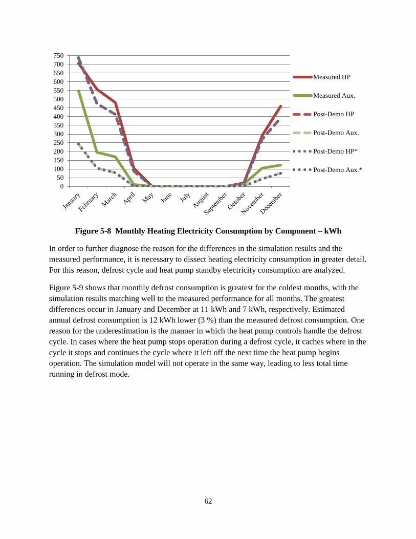
62

Figure 5-8 Monthly Heating Electricity Consumption by Component – kWh

In order to further diagnose the reason for the differences in the simulation results and the

measured performance, it is necessary to dissect heating electricity consumption in greater detail.

For this reason, defrost cycle and heat pump standby electricity consumption are analyzed.

Figure 5-9 shows that monthly defrost consumption is greatest for the coldest months, with the

simulation results matching well to the measured performance for all months. The greatest

differences occur in January and December at 11 kWh and 7 kWh, respectively. Estimated

annual defrost consumption is 12 kWh lower (3 %) than the measured defrost consumption. One

reason for the underestimation is the manner in which the heat pump controls handle the defrost

cycle. In cases where the heat pump stops operation during a defrost cycle, it caches where in the

cycle it stops and continues the cycle where it left off the next time the heat pump begins

operation. The simulation model will not operate in the same way, leading to less total time

running in defrost mode.

0

50

100

150

200

250

300

350

400

450

500

550

600

650

700

750

Measured HP

Measured Aux.

Post-Demo HP

Post-Demo Aux.

Post-Demo HP*

Post-Demo Aux.*

63

Figure 5-9 Monthly Defrost Electricity Consumption – kWh

Standby energy consumption (see Figure 5-10) estimated by the simulation model maps well to

the measured consumption and varies by month, with the greatest standby energy consumed

during the mild seasons because the equipment is in operation less often, the greater the standby

electricity consumption. The simulation estimates are greater than the measured performance for

April through October and lower for November through March. The simulation underestimates

the amount of time for which cooling equipment is in operation and overestimates the amount of

time for which heating equipment is in operation. The estimated annual standby consumption is

8 kWh (3 %) greater than the measured standby consumption. Controlling for the 5 days of lost

data in August would decrease estimated standby electricity consumption by approximately

4 kWh to equal the measured standby consumption of 17 kWh.

Figure 5-10 Monthly Heat Pump Standby Electricity Consumption – kWh

125

99

64

2 2

43 75

136

99

65

1 2

38

82

0

20

40

60

80

100

120

140k

Wh

Post-Demo

Defrost

[kWh]

Measured

Defrost

[kWh]

1012

21

3432

2116

21

2734

25

2016

16 21

3231

16 13

17

23

32

26

21

0

5

10

15

20

25

30

35

Post-Demo

Standby

[kWh]

Measured

Standby

[kWh]

64

After analyzing consumption to meet the heating load of the NZERTF, it is apparent that the

simulation cannot replicate the operating conditions of the heat pump and electric resistance

auxiliary element discussed in Section 4.7. The operation controls of the heating components in

the NZERTF have been adjusted, and are currently being tested in a follow-up demonstration

phase. The capacity of the auxiliary resistive heating element has been reduced by half from

10 kWh to 5 kWh. Dehumidification control was shifted from the heat pump to a whole house

dehumidifier. The thermostat is currently being operated based on an average of the 1st floor and

2nd floor temperatures. Additionally, the HRV system is now cycling on at 0.057 m3/s

(120 CFM) for 40 minutes out of every hour, leading to an hourly average of 0.038 m3/s

(80 CFM). The post-demonstration phase simulation has been adjusted to account for the

reduction in the resistive heating capacity, and rerun with 2014 weather data (AMY for KGAI

weather station) to determine if the simulation effectively replicates the new controls for meeting

the heating load of the NZERTF for October through December of 2014.

Figure 5-11 compares the post-demonstration phase simulation results to the measured

performance for the heating and cooling system (excluding the dehumidifiers) during October

through December of 2014. The post-demonstration phase simulation results more closely align

with the measured consumption, with minimal overestimation in October (3 kWh or 3 %) and an

underestimation in November (27 kWh or 9 %) and December (12 kWh or 3 %). Total

consumption estimated by the simulation for October through December is 834 kWh, which is

within 4 % of the measured consumption of 871 kWh. In contrast, the simulation underestimated

consumption for October through December of the demonstration phase (year 2013) by 206 kWh

or 20 %.

Figure 5-11 Updated Heating Electricity Consumption (2014) – kWh

84

326

460

87

299

448

0

50

100

150

200

250

300

350

400

450

500

October November December

kW

h

Measured

Sim - New

Controls

65

A disaggregated analysis is shown in Figure 5-12, where consumption by each component is

provided. Previously, the post-demonstration phase simulation model underestimated both the

heat pump and resistive heat electricity consumption in November and December. The new

model more closely matches the measured performance with the new NZERTF controls.

Estimated heat pump consumption is 51 kWh (6 %) lower than the measured heat pump

consumption for October 2014 through December 2014. The heat pump is not operating as often

in the simulation model, leading to greater standby electricity consumption (6 kWh or 8 %)

relative to the measured consumption. Auxiliary resistive heat is not operated for heating the

NZERTF throughout the 3 months, and is operated only during defrost cycles. The model

overestimates defrost electricity consumption by 14 kWh (44 %). Based on these results, it is

reasonable to assume that the new simulation model is now sufficiently replicating the

performance of the HVAC system.

Figure 5-12 Updated Heating Electricity Consumption by Component – kWh

Figure 5-13 shows electricity consumption for the HRV system. The adjustment made to the

post-demonstration phase simulation (shift in electric power between zone-level HRVs) only

impacted estimated consumption of the HRV system for 11 of 12 months, which overestimates

consumption relative to the measured performance. The dip in the measured data in August is a

result of the missing data for August 2 through August 6, which can be seen in the

pre-demonstration phase simulation (with faults) result.

840789

31 45 29 4574 80

0

100

200

300

400

500

600

700

800

Measured Sim - New

Controls

Measured Sim - New

Controls

Measured Sim - New

Controls

Measured Sim - New

Controls

Heat Pump Auxiliary Resistive Defrost Standby

kW

h

66

Figure 5-13 HRV Electricity Consumption by Month - kWh

5.5 Domestic Hot Water Electricity Consumption

Figure 5-14 shows measured consumption and results for the pre-demonstration phase

(Pre-Demo Phase), post-demonstration phase (Post-Demo Phase), and post-demonstration phase

with operation faults and changes to piping (shortening and improved insulation of the piping

between the two tanks) made on September 26 (denoted as “Post-Demo Phase**”). The

adjustments in the post-demonstration phase simulation for both DHW demand and performance

specifications significantly increased the solar loop pump electricity consumption, which maps

well to the measured performance except for July and August. The heat pump water heater

electricity consumption (combination of consumption by the heat pump and electric resistance

auxiliary element internal to the heat pump water heater tank) increases for all months from the

adjustments in the post-demonstration phase simulation (Post-Demo Phase). Monthly

consumption is similar to the measured performance for February through May, but is

consistently low for June through January with the largest underestimation occurring in July and

August.

After accounting for the faulty operation of the heat pump and solar loop pumps and the issues

related to the piping between tanks in Post-Demo Phase**, electricity consumption for the heat

pump water heater increases for most months. The largest increases occur in August and

September due to the inoperability of the solar loop pumps in late August and early September

and the longer piping and poor insulation on plumbing between July 1 and September 26.

Consumption increases in November and December due to inoperability of the heat pump in late

November and early December, causing greater demand on the less efficient electric resistance

auxiliary heating element in the water heater tank. The solar loop pump electricity consumption

in Post-Demo Phase** maps well to the measured solar loop pump consumption.

05

101520253035404550

kW

hPre-Demonstration

Phase

Measured

Post-Demonstration

Phase

Post-Demonstration

Phase*

67

Figure 5-14 Heat Pump Water Heater and Pump Electricity Use (kWh) – Monthly

Two reasons for the lower estimated consumption have been identified, although cannot be

addressed at this time. The first reason is the rated COP and associated efficiency performance

curve of the heat pump water heater. The model may not effectively capture the reduction in

efficiency of the heat pump as the temperature of the water entering the water heater increases

due to the water pre-heating by the solar thermal system. The second reason is that simulation

models are restricted in their ability to replicate the water draws (hot and cold) because the

operation of the NZERTF leads to water draws that are shorter than the minimum allowed one

minute simulation timestep. Since the simulation assumes fewer, longer water draws to meet the

target water consumption, the demand profile on the water heater will be different.

The pre-heated solar tank and heat pump water heater tank temperatures are shown in Figure

5-15. The change from the stratified tank and mixed tank objects in the post-demonstration phase

simulation leads to the measured tank temperature to be lower than the temperature measured at

the outlet of the pre-heated solar storage tank. Accounting for the inoperability of the solar loop

pumps leads to a drop in the tank temperature in the simulation for August, which mirrors the

drop in the measured tank temperature.

0

10

20

30

40

50

60

70

80

90

100

110

120

130

140

150

160k

Wh

Pre-Demo Phase -

Water Heater

Pre-Demo Phase -

Solar Loop Pumps

Measured - Water

Heater

Measured - Solar Loop

Pumps

Post-Demo Phase -

Water Heater

Post-Demo Phase -

Solar Loop Pumps

Post-Demo Phase** -

Water Heater

Post-Demo Phase** -

Solar Loop Pumps

68

Figure 5-15 DHW Tank Average Water Temperatures (°C) – Monthly

5.6 Domestic Water Consumption

Figure 5-16 shows that all five DHW demand categories were adjusted in volume of total water

drawn (hot and cold) in the post-demonstration phase simulation. Total water consumption in the

post-demonstration phase simulation is 324 L (85.5 gallons) per day, which is 7 L (1.8 gallons)

per day greater than measured water consumption (317 L or 83.7 gallons). The flow rates were

decreased for sink draws and increased for shower, bath, clothes washer, and dishwasher draws.

After accounting for faulty operation of the clothes washer, estimated consumption exactly

matches the measured consumption. The simulation models are restricted in their ability to

replicate the water draws (hot and cold) because the operation of the NZERTF leads to water

draws that are shorter than the minimum allowed one minute simulation timestep, which may

impact the end uses of both water volume and electricity consumption.

0

5

10

15

20

25

30

35

40

45

50

55T

emp

era

ture

[°C

]Pre-Demonstration

Phase HPWH Tank

Pre-Demonstration

Phase Solar Tank

Post-Demonstration

Phase HPWH Tank

Post-Demonstration

Phase Solar Tank

Measured HPWH

Tank

Measured Solar

Tank

Post-Demonstration

Phase** HPWH

Tank

Post-Demonstration

Phase** Solar Tank

69

Figure 5-16 Daily DHW Water Consumption – Gallons per Day14

5.7 Solar Photovoltaic Generation

Figure 5-17 shows the electricity production for each of the three simulations and the measured

performance. The estimated production better matches the measured performance once the

simulation accounts for the missing measured data in July, August, and December. The most

significant adjustment is realized for August because there were five days of missing data while

there were only two days in December and one day in July. The overestimation of production

during February, March, and November may be a result of the variation in snow cover on the PV

panels during and after the uncommon snowstorms during those months. It is possible that the

data collection equipment at the local weather station experienced snow cover for a shorter

period of time than the PV panels on the NZERTF, either due to quicker melting or manual

instrument cleaning. An approach that could help to resolve any differences is to incorporate

solar irradiance data collected at the NZERTF into the AMY file.

14 1 gallon = 3.7854 L

0

5

10

15

20

25

30

35

40

45

Dishwasher Clothes Washer Sink Showers Baths

Ga

llo

ns

Pre-

Demonstration

Phase

Post-

Demonstration

Phase

Post-

Demonstration

Phase*

Measured

70

Figure 5-17 Total Solar PV Electricity Production (kWh) - Monthly

0

200

400

600

800

1000

1200

1400

1600

1800k

Wh

Pre-

Demonstration

Phase

Post-

Demonstration

Phase

Post-

Demonstration

Phase*

Measured

71

6 Limitations

Whole building energy simulation software is limited in its abilities to estimate real world energy

performance for a number of reasons. It is difficult to control for all potential variables that can

impact the thermal conditions in a building and the resulting operation of equipment to meet the

needs of the occupants. There are a number of reasons that the estimated performance from the

E+ model may vary from the actual performance of the NZERTF. A few are discussed below.

First, air infiltration may not be accurately estimated in the E+ models. The infiltration rate due

to building envelope leakage in the E+ model is simplified to an ELA based on a recent air

leakage test. However, this infiltration will not match actual infiltration because the infiltration

rate will differ depending on the outdoor weather conditions, relative pressure in the building,

and location of the leakage areas. The E+ model currently does not control for these factors.

Second, discrepancies between the E+ model and the actual NZERTF design are the most

prominent reasons for variations in energy performance. The E+ model does not include the

stairway/foyer opening, which restricts thermal transfer between the floors and increases the

conditioned floor area relative to the actual NZERTF design. The greater conditioned floor area

will impact the thermal load needed to meet the thermostat set points as well as the minimum

ventilation rates required for the HVAC equipment.

Third, E+ cannot directly replicate some of the currently installed building equipment or the

actual operation schedules. The whole house ventilation system was simulated using two zone-

level systems. The dehumidify-only mode for the air-to-air heat pump was simulated using

zone-level dehumidifiers. The current model could not directly simulate the close-looped nature

of the solar thermal system. The sink water draws during the demonstration phase were less than

one minute in length, which is shorter than the allowed timestep in E+. The dynamics of the

domestic hot water demands cannot be accurately replicated in the simulation design, including

short water draws (less than one minute), varying water draw temperatures, and intermittent

water draws during dishwasher and clothes washer cleaning cycles. The model does not account

for any non-simulated occupant-related infiltration and heat loads, such as researchers and tours

entering, occupying, and leaving the NZERTF. There is a lack of data associated with the

efficiency of the heat pump water heater because the water temperature entering the heat pump

was not measured during the demonstration phase. There may be additional faults or missing

data beyond those discussed in this document that has not yet been accounted for in the

simulation model. All of these factors can lead to uncertainty in the model results.

Fourth, the AMY weather file may not reflect exactly the same conditions as those experienced

by the NZERTF. Weather can vary across the five mile distance between the NIST campus and

the KGAI weather station. The equipment used to collect weather data at the KGAI weather

station may not accurately measure some of the variables reported in the AMY file, such as snow

cover.

72

These limitations will be addressed whenever possible to improve the accuracy of the E+

simulation results in future research. However, there is a balancing act between complexity and

accuracy in simulation model design. It is important to determine what level of accuracy is

considered precise enough for the model to be considered “validated.”

73

7 Discussion and Future Research

The estimated performance of the NZERTF based on the pre-demonstration phase simulation

model differed from the measured performance during the demonstration phase for five main

reasons. First, the initial simulation assumptions were incorrect due to a lack of information on

the specifications of the installed equipment. Second, where information was lacking,

conservative parameter values were used in the model in order to not underestimate

consumption. Third, there was an inability to directly model some of the installed equipment in

the software. Fourth, the operation schedules and controls of the NZERTF were adjusted

throughout the preparation for the demonstration phase. Finally, there were faults and

adjustments in the operation of the NZERTF during the demonstration phase.

A detailed review of the simulation assumptions and the measured data from the demonstration

phase was completed in order to identify what adjustments should be made to the simulation

model to better replicate the operation of the NZERTF during the demonstration phase. The

resulting post-demonstration phase simulation leads to results that more closely match the

measured performance, within 4 % of total electricity consumption and 3 % of electricity

production.

The post-demonstration phase model does not closely replicate the electricity consumption to

meet the heating load for the NZERTF during the demonstration phase of the NZERTF because

of the manner in which the heating equipment is operated. The simulation model's heating

equipment operation is based on the capability of the equipment to meet the heating load, while

the installed heating equipment operated based on time-oriented controls in the installed

thermostat. The time-based controls led the electric resistance auxiliary heating element to

operate at times when the heat pump was effectively increasing the room temperature

(maintaining “comfortable” occupant conditions) but when the setpoint temperature was not

achieved quickly enough. As a result, the electric resistance auxiliary element consumed

1162 kWh while the simulated consumption was estimated to be 547 kWh. The NZERTF is

currently in a second demonstration phase, which includes changes to the operating controls for

the heating equipment. Measured data for October 2014 through December 2014 and associated

weather data is used to rerun the simulation, and shows that estimated heating- and cooling-

related electricity consumption is within 4 % of measured consumption. Given the new heating

operation controls for the NZERTF, the validated post-demonstration phase simulation is

effective at replicating the measured performance.

Issues experienced during the demonstration phase lead to many of the remaining differences

between the post-demonstration phase simulation and the measured performance. There were

several instances for which data collection errors occurred, which impacted all building systems

(HVAC, DHW, solar thermal, and solar PV). Faults in equipment operation led to differences in

the HVAC, DHW, and solar thermal systems. After accounting for the most significant faults

74

and data collection issues, the simulation results are even closer to the measured performance

during the demonstration phase.

The validated post-demonstration phase model does not identically replicate the NZERTF

experimental operation. Estimated heat pump consumption is marginally lower than the

measured consumption, which could be driven by factors that are directly related to the heat

pump parameter values and indirectly related to heat pump operation through the integrated

aspects of building components. Similarly, the DHW system underestimates consumption, which

may be due to the assumed COP of the heat pump water heater. There was not data collected

during the demonstration phase that could determine the performance of the heat pump water

heater based on the difference in entering water temperature.

The post-demonstration phase simulation model will be useful to assist in research in a number

of areas, both directly related to the NZERTF demonstration phase as well as future, broader

research topics. The results from the post-demonstration phase simulation and the detailed

database collected from the demonstration phase can be used to analyze the relative performance

of the simulation to experimental results for each individual building component: building

envelope, HVAC system, DHW system, solar thermal system, and solar PV system. The detailed

analysis of these systems can assist in determining the parameters that are necessary for the

model to have relatively accurate results. Additionally, the level of accuracy can be weighted

with the time and effort required to determine the diminishing returns of such accuracy, allowing

modelers to determine the required level of accuracy given their ultimate goals.

The simulation model can be used to make relative comparisons of the NZERTF to alternative

building designs. The most obvious comparison would be to an identical house that meets the

Maryland state energy code for residential buildings. The energy performance savings can be

compared to the additional costs of the efficiency improvements. Sensitivity analysis can be used

to look at a number of interesting research areas. Sensitivity analysis can look at the incremental

changes between the Maryland code compliant house and the NZERTF to determine which

energy efficiency measures result in the greatest energy reductions, the most cost-effective

measures, and how energy efficiency measures interact. The validated simulation model can be

used to test the sensitivity of the NZERTF performance to varying weather conditions by using

historical weather data (annual AMY for the past 30 years). The simulation model can also be

altered to determine how additional energy efficiency measures would impact the energy

performance of the NZERTF, including equipment that is already installed in the NZERTF. For

example, each of the three geothermal heat pump systems could be included in the analysis to

determine the impacts of systems on the NZERTF’s energy performance. Occupant behavior can

be altered to determine how sensitive the results are to the assumed occupant activity. Natural

ventilation could be introduced by opening and closing windows based on the outdoor

temperature to account for common human behavior.

75

References

ASHRAE Fundamentals, 2012, American Society of Heating, Refrigerating and Air-

Conditioning Engineers, Inc., www.ashrae.org.

ASHRAE Standard 90.2, 2007, American Society of Heating, Refrigerating and Air-

Conditioning Engineers, Inc., www.ashrae.org.

Building Science Corporation. 2009. 65 % Net Zero Energy Residential Test Facility

Construction Documents Set.

Christensen, D. and Winkler, J. December 2009. Laboratory Test Report for ThermaStor Ultra-

Aire XT150H. NREL Technical Report NREL/TP-550-47215.

Davis, M, Healy, W., Boyd, M., Ng, Lisa, Payne, V., Skye, H., Ullah, T., 2014, Monitoring

Techniques for the Net-Zero Energy Residential Test Facility, National Institute of

Standards and Technology, NIST Technical Note 1854, DOI:

http://dx.doi.org/10.6028/NIST.TN.1854.

Department of Energy (DOE), 2013, Building Technologies Program, EnergyPlus energy

simulation software Version 8.0.0, http://apps1.eere.energy.gov/buildings/energyplus/.

Energy Star. 2012, Product databases for clothes washers, dishwashers, and refrigerators.

http://www.energystar.gov/index.cfm?c=products.pr_find_es_products

Everyday Green, 2012, Building Leakage Test of the Net Zero Energy Residential Facility.

Fanney, Hunter et al., 2015, Net-Zero and Beyond! Design and Performance of NIST’s Net-Zero

Energy Residential Test Facility, Energy and Buildings, currently in revisions.

Heliodyne, 2008, HPak Systems Installation Guide. www.heliodyne.com.

Heliodyne, 2008, Solar Hot Water Technical Specifications. www.heliodyne.com.

Hendron, R., Engebrecht, C., September 2010, Building America house simulation protocols,

National Renewable Energy Laboratory, Building Technologies Program.

Hubbell, 2011, Heat Pump Water Heater Model PBX specifications.

http://www.hubbellheaters.com/model/pbx/.

Kneifel, Joshua, October 2012, Annual Whole Building Energy Simulation of the NIST Net Zero

Energy Residential Test Facility Design, NIST TN 1767, DOI:

http://dx.doi.org/10.6028/NIST.TN.1767.

http://www.ashrae.org/

http://www.ashrae.org/

http://apps1.eere.energy.gov/buildings/energyplus/

http://www.energystar.gov/index.cfm?c=products.pr_find_es_products

http://www.heliodyne.com/

http://www.heliodyne.com/

http://www.hubbellheaters.com/model/pbx/

http://dx.doi.org/10.6028/NIST.TN.1767

76

Kneifel, Joshua, September 2013, Energy Performance of the NIST Net Zero Energy Residential

Test Facility Relative to a Maryland Code- Compliant Design, NIST TN 1166.

Kneifel, Joshua, June 2014, Life-Cycle Cost Comparison of the NIST Net Zero Energy

Residential Test Facility to a Maryland Code-Compliant Design, NIST SP 1172. DOI:

http://dx.doi.org/10.6028/NIST.SP.1172.

Lstiburek, Joseph, 2010, Building Science Corporation. BSI-030: Advanced Framing. Building

Science Insights. http://www.buildingscience.com/documents/insights/bsi-030-advanced-

framing/#F04

Omar, Farhad and Bushby, Steven. November 2013. Simulating Occupancy in The NIST Net-

Zero Energy Residential Test Facility. NIST Technical Note 1817.

Petit, Betsy et al., 2015, Design Challenges of the NIST Net Zero Energy Residential Test

Facility, NIST Technical Note 1847.

Sunpower 320 solar photovoltaic panel specifications. 2011. www.sunpower.com.

Sunpower 5000m inverter specifications. 2011. www.sunpower.com.

Ultra-Aire 65H Ventilating Dehumidifier specifications. 2011. www.Ultra-Aire.com.

Venmar AVS HRV EKO 1.5 specifications. 2009. http://www.venmar.ca/en/product/root-

category/air-exchangers/venmar-avs/products/eko-15-hrv-

_124.aspx?id_page_parent=775.

Solar Rating and Certification Corporation (SRCC). 2014, Certified Solar Collector Rating for

Heliodyne GOBI 406 001, http://www.solar-rating.org/index.html.

Weather Analytics, 2014, Actual Meteorological Year (AMY) formatted weather data for July 1,

2013 through June 30, 2014.


http://www.buildingscience.com/documents/insights/bsi-030-advanced-framing/#F04

http://www.buildingscience.com/documents/insights/bsi-030-advanced-framing/#F04

http://www.sunpower.com/

http://www.sunpower.com/

http://www.ultra-aire.com/

http://www.venmar.ca/en/product/root-category/air-exchangers/venmar-avs/products/eko-15-hrv-_124.aspx?id_page_parent=775



http://www.solar-rating.org/index.html