simulated-annealing-based conditional simulation for the

Journal of Applied Geophysics 68 (2009) 60–70

Contents lists available at ScienceDirect

Journal of Applied Geophysics

j ourna l homepage: www.e lsev ie r.com/ locate / jappgeo

Simulated-annealing-based conditional simulation for the local-scalecharacterization of heterogeneous aquifers

B. Dafflon, J. Irving, K. Holliger ⁎Institute of Geophysics, University of Lausanne, CH-1015 Lausanne, Switzerland

⁎ Corresponding author. Tel.: +41 21 692 44 03; fax:E-mail address: [email protected] (K. Holliger).

0926-9851/$ – see front matter © 2008 Elsevier B.V. Adoi:10.1016/j.jappgeo.2008.09.010

a b s t r a c t
a r t i c l e i n f o
Article history:
Simulated-annealing-based Received 31 October 2007Accepted 19 September 2008
Keywords:Data integrationGeoradarSimulated annealingStochastic methodsPorosityConditional simulation

conditional simulations provide a flexible means of quantitatively integratingdiverse types of subsurface data. Although such techniques are being increasingly used in hydrocarbonreservoir characterization studies, their potential in environmental, engineering and hydrological investiga-tions is still largely unexploited. Here, we introduce a novel simulated annealing (SA) algorithm gearedtowards the integration of high-resolution geophysical and hydrological data which, compared to moreconventional approaches, provides significant advancements in theway that large-scale structural informationin the geophysical data is accounted for. Model perturbations in the annealing procedure aremade by drawingfrom a probability distribution for the target parameter conditioned to the geophysical data. This is the onlyplace where geophysical information is utilized in our algorithm, which is in marked contrast to otherapproaches where model perturbations are made through the swapping of values in the simulation grid andagreement with soft data is enforced through a correlation coefficient constraint. Anothermajor feature of ouralgorithm is the way in which available geostatistical information is utilized. Instead of constrainingrealizations to match a parametric target covariance model over a wide range of spatial lags, we constrain therealizations only at smaller lagswhere the available geophysical data cannot provide enough information. Thuswe allow the larger-scale subsurface features resolved by the geophysical data to havemuchmore due controlon the output realizations. Further, since the only component of the SA objective function required in ourapproach is a covariance constraint at small lags, our method has improved convergence and computationalefficiency over more traditional methods. Here, we present the results of applying our algorithm to theintegration of porosity log and tomographic crosshole georadar data to generate stochastic realizations of thelocal-scale porosity structure. Our procedure is first tested on a synthetic data set, and then applied to datacollected at the Boise Hydrogeophysical Research Site.

© 2008 Elsevier B.V. All rights reserved.

1. Introduction

A key control on groundwater flow and contaminant transport inthe subsurface is the spatial distribution of hydrological properties.Accurate characterization of these properties is crucial for developingreliable numerical models of flow and transport, which are required todesign effective and cost-efficient aquifer remediation and ground-water management strategies. It is well understood that spatialvariability needs to be defined at a wide range of scales for effectivemodeling of hydrological phenomena (e.g., Sudicky and Huyakorn,1991; Gelhar, 1993; Zheng and Gorelick, 2003; Hubbard and Rubin,2005). However, conventional hydrological measurement techniquestend to lie at two ends of a spectrum in terms of resolution andsampling volume, leaving a significant gap in a range that is expectedto contain particularly critical hydrological information. Whereaspumping and tracer tests tend to yield only gross average properties

+41 21 692 44 05.

ll rights reserved.

over a relatively large region, core samples and borehole logs yieldhigh-resolution estimates of aquifer properties, but only along sparse1-D profiles. Consequently, over the past two decades, much work hasbeen done on the use of geophysical methods for aquifer character-ization. Such methods can bridge the gap between the analysis ofcores or logs and well tests, and have proven to be extremely usefulnot only for aquifer zonation but also for estimating the spatialdistribution of hydrological parameters (e.g., McKenna and Poeter,1995; Hyndman et al., 2000; Chen et al., 2001; Tronicke et al., 2002;Hubbard and Rubin, 2005; Kowalsky et al., 2005; Paasche et al., 2006).An important and still largely unresolved issue with the use ofgeophysical data in hydrological studies, however, is that of dataintegration. That is, how do we quantitatively integrate geophysicaldata with an existing database of other measurements to bestconstrain our knowledge of the spatial distribution of one or severaltarget parameters?

The integration of different types of data for subsurface character-ization has been a subject of much investigation in the petroleumindustry, and has received increased attention in groundwater studies

mailto:[email protected]

http://dx.doi.org/10.1016/j.jappgeo.2008.09.010

http://www.sciencedirect.com/science/journal/09269851

Fig. 1. Flowchart of SA approach for conditional stochastic simulation.

61B. Dafflon et al. / Journal of Applied Geophysics 68 (2009) 60–70

in recent years. Whereas much data integration and joint inversionwork in the past has involved the determination of a single model ofthe subsurface parameters of interest, a number of recent efforts havefocused on the creation of sets of multiple realizations that areconsistent with all of the available data, and represent the uncertaintyin our knowledge of the spatial distribution of subsurface properties(e.g., McKenna and Poeter, 1995; Bosch, 1999; Avseth et al., 2001;Caers et al., 2001; Mukerji et al., 2001; Ramirez et al., 2005; Hansenet al., 2006). The idea behind such conditional simulation approachesis that they can be used in combination with complex hydrologicalmodels to make predictions regarding groundwater flow andcontaminant transport within a framework of uncertainty. Workwith thesemethodologies has increased over recent years as a productof continually growing computer capacity, and also the ever increasingrealization that “mean models” of subsurface properties do notadequately represent subsurface heterogeneity for reliable flow andtransport predictions (e.g., Goovaerts, 1997).

Due to their inherent flexibility with regard to imposing constraintsand their conceptual simplicity, simulated-annealing-type conditionalstochastic simulations seem to be particularly promising for subsurfacedata integration (e.g., Deutsch and Wen, 1998, 2000; Kelkar and Perez,2002). The simulated annealing (SA) approach is not limited to simpleGaussian statistics, and is able to incorporate any constraint on theoutput realizations that can be expressed in the form of an objectivefunction, with the caveat that efficiency in terms of computation timeand convergence decreases with constraint complexity. With SA,parameter fields satisfying all of the available data are obtained throughminimization of a global, generally multi-component objective function,and multiple realizations can be generated by running the algorithmwith different initial conditions. It should be emphasized that thevariability seen in such multiple realizations depends on the appliedconstraints and stopping criteria, and as a result the realizations shouldnot be confusedwith samples drawn fromaposterior probability densityfunction. Nevertheless, the SA method still allows evaluation of thevariability in flow and transport behavior associatedwith uncertain dataand constraints.

Recently, Tronicke and Holliger (2005) explored the use of SA forhydrogeophysical data integration through a synthetic model study.Starting with a simulated porosity model of a heterogeneous alluvialaquifer, they generated synthetic porosity logs and crosshole georadartraveltime data. These data, along with geostatistical constraints, werethen used as conditioning information in a SA-based optimizationprocedure to generate porosity models that were consistent with all ofthe available information. In their work, Tronicke and Holliger (2005)pursued the classical SA approach of gradually “organizing” anuncorrelated random initial field through repeated swapping of valuesin the simulation grid, while adherence to the geophysical andgeostatistical data was accomplished through matching the correlationcoefficient between the realization and geophysical data to a prescribedvalue, and matching a prior parametric covariance model, respectively.Although the results obtained using this methodology clearly demon-strated that SA has much potential for hydrogeophysical data integra-tion, we have found that the lateral continuity of the resulting porositymodels is in general inadequate, which in turn significantly reduces thepredictive value of such models in subsequent flow and transportsimulations. Closer inspection indicates that this problem likely arisesfrom the fact that it is inherently difficult with purely stochasticsimulations to effectively impose constraints with regard to theunderlying deterministic structure of the target parameter, as provided,for example, by high-resolution geophysical data.

In this paper, we present a novel SA-type conditional simulationprocedure that aims to address and resolve this issue, as well as toimprove the convergence and computational efficiency of thetraditional SA method, which are known to be suboptimal as a resultof having a relatively complex objective function. To begin, we reviewthe overall methodology and describe an approach to more effectively

account for the larger-scale deterministic information contained ingeophysical data. Next, we test our conditional stochastic simulationalgorithm on a synthetic data set consisting of crosshole georadar dataand porosity logs from a highly heterogeneous, realistic aquifermodel.Finally, we use our method to integrate field crosshole georadar andneutron porosity log data collected at the Boise HydrogeophysicalResearch Site (BHRS) near Boise, Idaho, USA.

2. Conditional stochastic simulation using simulated annealing

2.1. Background

Simulated annealing is a directional Monte-Carlo-type optimizationprocedure, whose central idea is based upon the thermodynamics of acooling melt. Atoms can move freely throughout a melt at high temper-atures, but as the temperature is lowered, their mobility progressivelydecreases. Eventually, the system reaches its thermodynamic minimum-energy state and the atoms assumefixed positionswithin a crystal lattice.In SA, there are a large number of possible initial states, but during thecooling or annealing process all possible states converge to a finalacceptable one. Aflowchart describing the generalmethodology of SA forconditional simulation is shown in Fig. 1 (e.g., Deutsch, 2002; Kelkar andPerez, 2002; Tronicke and Holliger, 2005). The classical approach beginswith an uncorrelated random field generated from an inferred/assumedprobability distribution for the target parameter. The optimizationprocess that follows consists of repeatedly perturbing individual valuesof this randomfield inorder to satisfya global objective function,O,whichgenerally consists of the weighted sum of several component objectivefunctionsOi that represent constraints on fitting the output realization tothe available data or information:

O =Xni=1

ωiOi; ð1Þ

where n is the number of component objective functions and ωi arethe weights. All perturbations that lower the global objective functionare accepted in the algorithm, whereas those that do not are acceptedaccording to a Boltzmann-type exponential probability distributioncontrolled by a temperature parameter T. This “decision rule” is

62 B. Dafflon et al. / Journal of Applied Geophysics 68 (2009) 60–70

generally quantified in terms of the acceptance probability p of a givenconfiguration:

p =1; if OnewbOold

expOold − Onew

T

� �; otherwise:

8<: ð2Þ

The higher the temperature parameter T, the more likely anunfavorable perturbation will be accepted. Throughout the annealingprocess, the temperature is lowered gradually such that themodel hasa chance to reach an optimal energy state. Once the global objectivefunction is deemed small enough, the SA process is terminated.

In the work of Tronicke and Holliger (2005) exploring the use of SAfor hydrogeophysical data integration, the global objective functionconsisted of three components: the first controlled the reproduction of aspecified covariancemodel for the porosity distribution to be simulated(inherentlyassuming stationarityandenforcingadherence to thismodelat awide range of spatial lags), the second the reproduction of boreholeporosity log data, and the third the conditioning of the simulatedporosity field to the tomographic crosshole georadar image using a pre-defined target correlation coefficient between these quantities. Modelperturbations during the SA procedure were made through theswapping of randomvalues in the grid, whichmeant that the histogramof the original random realization did not change during the optimiza-tion procedure. Although, as mentioned previously, this work stronglydemonstrated the potential of the SA method for generating aquifermodels honoring a variety of data and prior information, it has becomeclear through further numerical studies that informationwith regard tothe larger-scale subsurface structure, as provided by the geophysicaldata, is inadequately exploited, which in turn results in porosity modelsthat are sub-optimal with regard to their internal structure and realism.

We believe that the above difficulty arises for a number of reasons.First is the issue of constraining theoutput porositymodel to correspondto the geophysical image using only a single parameter, namely aprescribed correlation coefficient between these two quantities. Indoing this, a rigid and arguably rather simplistic prior assumption ismade about the relation between the geophysical data and the targetparameter, which in many cases may be in error and cause difficultieswith incorporating the geophysical information. One can imagine itbeing very difficultwith a single parameter constraint to ensure that theaccurate large-scale subsurface structural information provided by ageophysical image is properly retained in the output realizations. Asecond reason that we suspect contributes to the inadequate incorpora-tion of large-scale geophysical information in the SAmethod of Tronickeand Holliger (2005) is the updating of the model through the swappingof values in the simulation grid. This implies the use of a pre-determinedglobal probability density function for the target parameter, which isgenerally unknown and may be at odds with the information providedby the geophysics. Finally is the issue of constraining the experimentalcovariance of the output realizations to match a target covariancefunction over a wide range of lags. In doing this at large lags, adherenceto larger-scale stochastic information is enforced, which in many casesmay contradict the more accurate deterministic information containedin the geophysical image. In other words, because of our very limitedknowledge of the true experimental covariance function at large lags,this constraint may force the output realizations to match an inaccuratecovariance model, and thereby go against the large-scale informationprovided by the geophysical data.

2.2. Accounting for large-scale structural information

Given the above observations, our goal was to develop a newapproach to SA-based conditional simulation that allows us to moresuitably incorporate the larger-scale structural information contained ina geophysical image. The key concept in this approach is that high-resolution geophysical images, such as crosshole georadar or seismic

tomograms, have as-of-yet largely unexploited potential in theconditioning of a model based on simulated annealing. In the following,we briefly outline our methodology.

2.2.1. Perturb the model by drawing from a conditional distribution forthe target parameter, given the available data

One key element of our new SA algorithm is the means by whichwe perturb the model and incorporate the geophysical and boreholelog data into the output realizations. Instead of randomly swappingvalues in the simulation grid, we perturb themodel by drawing from aconditional probability distribution for the target parameter, giventhese data (Deutsch and Wen, 1998). In other words, each perturba-tion step consists of drawing a random value from a conditionaldistribution, which can be defined for each cell of the model. Thisdistribution is obtained given the available geophysical or log data andtheir relation to the target parameter, and provides the only means bywhich these data are incorporated into the simulation procedure.Around the boreholes the conditional distribution is obtained fromthe log data and their estimated uncertainty. Away from the bore-holes, it is estimated from the geophysical data and their relation tothe target parameter.

The above means of perturbing the model has several advantages incomparison to the traditional SA approach. In particular, it avoids theproblem of requiring a priori the probability density function of the targetparameter, and it offers significantly more flexibility in accounting forspecific aspects and/or details of the geophysical information. Forexample, spatially dependent relationships consistent with varyingdegrees of local information can be readily incorporated into thesimulation process without the need for objective functions to constrainthe realizations to fit the different sources of information. The latter is ofsignificant practical importance as it greatly contributes to the simplifica-tion of our global objective function, which in turn significantly improvesthe algorithm's convergence and computational efficiency (Deutsch andWen, 1998; Parks et al., 2000).

The question of how to best determine the conditional distributionfor a particular target parameter with regard to geophysical data iscurrently receiving a significant amount of interest in a variety ofdomains (e.g., Ezzedine et al., 1999; Avseth et al., 2001; Chen et al.,2001; Bachrach, 2006). Although for hydrogeophysical applicationsthe simplest approach is to attempt to relate the parameters usinglaboratory-derived petrophysical relationships, such relationships areusually only valid at the small scale, and tend to encounter problemswhen they are used to “convert” geophysical images to true subsurfaceproperties. In an attempt to address this problem,Moysey et al. (2005)developed a Monte-Carlo approach involving numerical forwardmodeling to upscale petrophysical relationships from the laboratoryscale to the scale of a geophysical survey. Day-Lewis et al. (2005) alsoaddressed this issue by quantifying the correlation loss that occursbetween a geophysical image and model of subsurface properties as aresult of geophysical inversion. Another common method forestimating the conditional distribution for a hydrological parameterof interest given geophysical data, which we adopt in this paperbecause it is readily extended to field data and site-specific relation-ships, is to use collocated data sets along boreholes. Clearly, in thiscase, the quality of the estimated conditional relationship isdependent upon the number and quality of collocated data (e.g.,Ezzedine et al., 1999; Chen et al., 2001; Bachrach, 2006; Paasche et al.,2006).

2.2.2. Constrain realizations to parametric covariance model only at lagswhere the geophysical data do not provide enough information

The second key feature of our SA-type conditional simulationalgorithm is the way in which we account for available geostatisticalconstraints. Instead of using the common approach of forcing theoutput realizations to match a target parametric covariance modelover a wide range of spatial lags, we consider only those shorter lags

Fig. 2. (a) Synthetic porosity model representing a heterogeneous alluvial aquifer.(b) Result of tomographic inversion of the three, synthetic, crosshole georadar data setssimulated between boreholes located at 0, 10, 20 and 30 m lateral distance.


where this information is required because it is not provided by thegeophysical data.

It is well known that tomographic geophysical images can be viewedas smoothed versions of the corresponding true geophysical parameterfields.While being adequate representations of the underlying structureat larger-scales, such images lack information on the smaller-scalesubsurface structure. This information can be adequately provided bygeostatistical information regarding the parameter of interest. In our SAapproach, we only constrain the output realizations to a parametricgeostatistical model when necessary (i.e., at lags below the resolutionthreshold of the geophysical data), and we thus implicitly let thegeophysical data havemore control over the larger-scale structure of theoutput realizations. The choice of cut-off lag (i.e., the lag beyond whichwe do not constrain the output realizations to the target covariancemodel) must be chosen based on the estimated resolution of thegeophysical image. That is, at scales where the subsurface structure isdeemed to be not resolved by the geophysics, we should handle thevariability statistically. Similar to our use of a conditional distribution forperturbing the model as described above, this approach towardsgeostatistical constraints contributes to the simplification of the globalobjective function of our SA procedure and thus to improvedconvergence and computational efficiency. In fact, the only objectivefunction necessary in our algorithm involves constraining the outputrealization to the parametric covariancemodel at short lags. It should benoted that this procedure can be also viewed as effectively assigning avery high uncertainty to the target covariance function at large lags, thusallowing the geophysical data to control the large-scale structure in theoutput realizations. Clearly, using an approach that accounts for theergodic variability in the covariance function (e.g., Ortiz and Deutsch,2002;Hansen et al., 2008) in theSAobjective functionwould accomplisha similar goal.

3. Application to synthetic data

We now apply our SA-type conditional simulation algorithm to asynthetic example.Weuse the samedata thatwere used inTronicke andHolliger (2005) such that the potential advantages and limitations ofboth approaches can bemore easily identified. From an initial syntheticsubsurface porositymodel, crosshole georadar and neutron porosity logdatawere generated. The goal of the SA procedurewas then to integratethese two data types and produce, within the bounds of uncertaintydictated by the limited information, realizations of the underlyingporosity field. Crosshole georadar tomography has become a commontool for the detailed characterization of heterogeneous aquifers (e.g.,Chen et al., 2001; Hubbard et al., 2001; Tronicke et al., 2002; Tronickeet al., 2004). Its strong potential for complementing and enhancinghydrological characterization comes from its high sensitivity to watercontent and the high spatial resolution of themethod. We first describebelow how the synthetic data were generated, and then the applicationof our algorithm for the data integration.

3.1. Porosity model

TronickeandHolliger (2005)usedascale-invariantor “fractal”porositymodel, 30 m long and 16.5 m deep, that was characterized by a vonKármán covariance function (von Kármán, 1948; Goff and Jordan, 1988):

C hð Þ = σ2

2v−1C vð Þjh jah

� �v

Kvjh jah

� �; ð3Þ

where h is the lag vector, ah is the correlation length in the direction ofthe lag vector,σ is the standard deviation, Γ is the gamma function, andKν is the modified Bessel function of the second kind of order 0≤ν≤1,where ν is known as the Hurst number. The correlation length inEq. (3) is related to the outer range of scale-invariance. Fig. 2a showsthe synthetic porosity model that was generated from Eq. (3) using a

spectral simulation technique. Best-fitting von Kármán parameters tothe experimental variogram of this model are a ν-value of 0.2 andcorrelation length of 2 m in the vertical direction, and a ν-value of 0.3and correlation length of 10 m in the horizontal direction. Therealization has a mean porosity of 0.19 and standard deviation equal to0.03. All of these parameters can be regarded as typical of unconso-lidated clastic sediments consisting predominantly of sand and gravel(e.g., Gelhar, 1993; Heinz et al., 2003). The model is discretized at7.5 cm increments and boreholes are considered at lateral positions of0, 10, 20, and 30 m from the left model edge.

Key characteristics of the porosity model in Fig. 2a are that it isscale-invariant and thus characterized by strong heterogeneity atsmaller scales and quasi-deterministic features, such as the centralhigh-porosity channel, at larger scales. Having a ν-value close to zero,the model emulates the seemingly ubiquitous “flicker noise” behaviorcharacterizing virtually all petrophysical parameters including poros-ity (e.g., Walden and Hosken, 1985; Desbarats and Bachu, 1994; Hardyand Beier, 1994; Kelkar and Perez, 2002; Holliger and Goff, 2003) andcan thus be regarded as a challenging, pertinent and realistic test case.

3.2. Database

From the porosity model in Fig. 2a, synthetic borehole porosity logdata and crosshole georadar data were simulated. For the porosity logdata, vertical traces from the model at the defined borehole locationswere extracted. Consequently, the log data for this example are simplyunbiased in-situ measurements of the actual porosity at the boreholelocationswith a resolution on the order of a grid cell (7.5 cm). Althoughthis is clearly a simplification of real porosity log data, which willcontain a small amount of smoothing related to the support volume ofthe measurement, we feel that it is an adequate approximation for thepurpose of testing our approach.

To create the crosshole georadar data, three tomography surveyswere simulated between all adjacent pairs of wells in the syntheticmodel (i.e., between 0 and 10 m, 10 and 20 m, and 20 and 30 m).Together, the data from these surveys allow us to reconstruct thesubsurface velocity distribution in a series of panels having a width-to-depth ratio of approximately 0.66, which provides enough angularcoverage of the inter-borehole region for high resolution tomographicvelocity estimates (Williamson and Worthington, 1993). As a first

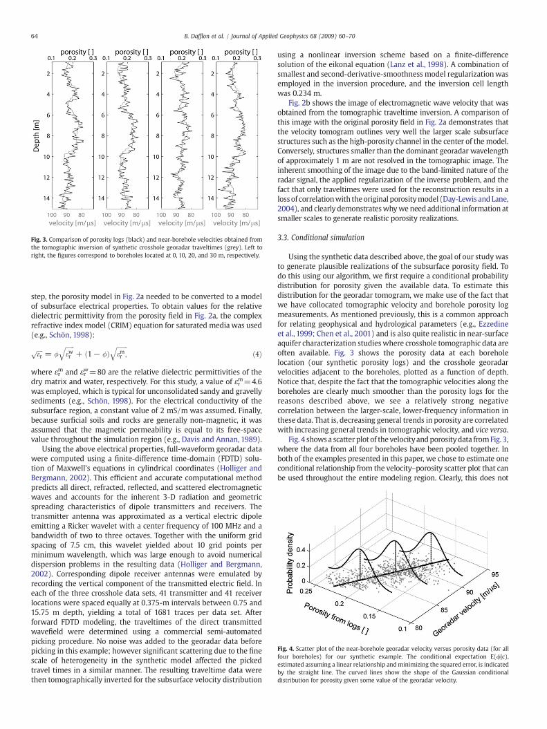
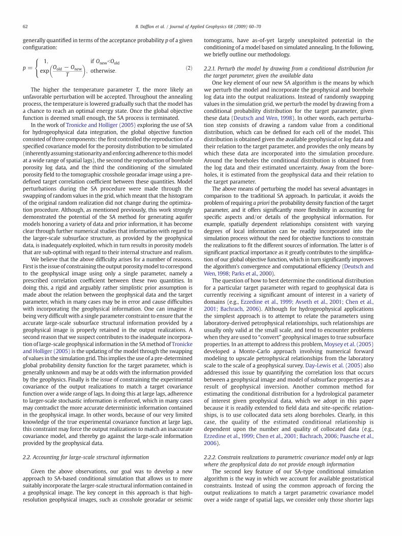
Fig. 3. Comparison of porosity logs (black) and near-borehole velocities obtained fromthe tomographic inversion of synthetic crosshole georadar traveltimes (grey). Left toright, the figures correspond to boreholes located at 0, 10, 20, and 30 m, respectively.

Fig. 4. Scatter plot of the near-borehole georadar velocity versus porosity data (for allfour boreholes) for our synthetic example. The conditional expectation E(ϕ|c),estimated assuming a linear relationship and minimizing the squared error, is indicatedby the straight line. The curved lines show the shape of the Gaussian conditionaldistribution for porosity given some value of the georadar velocity.


step, the porosity model in Fig. 2a needed to be converted to a modelof subsurface electrical properties. To obtain values for the relativedielectric permittivity from the porosity field in Fig. 2a, the complexrefractive index model (CRIM) equation for saturated media was used(e.g., Schön, 1998):

ffiffiffiffier

p= �

ffiffiffiffiffiffiewr

q+ 1− �ð Þ

ffiffiffiffiffiffiffiemr ;

qð4Þ

where εrm and εrw=80 are the relative dielectric permittivities of thedry matrix and water, respectively. For this study, a value of εrm=4.6was employed, which is typical for unconsolidated sandy and gravellysediments (e.g., Schön, 1998). For the electrical conductivity of thesubsurface region, a constant value of 2 mS/m was assumed. Finally,because surficial soils and rocks are generally non-magnetic, it wasassumed that the magnetic permeability is equal to its free-spacevalue throughout the simulation region (e.g., Davis and Annan, 1989).

Using the above electrical properties, full-waveform georadar datawere computed using a finite-difference time-domain (FDTD) solu-tion of Maxwell's equations in cylindrical coordinates (Holliger andBergmann, 2002). This efficient and accurate computational methodpredicts all direct, refracted, reflected, and scattered electromagneticwaves and accounts for the inherent 3-D radiation and geometricspreading characteristics of dipole transmitters and receivers. Thetransmitter antenna was approximated as a vertical electric dipoleemitting a Ricker wavelet with a center frequency of 100 MHz and abandwidth of two to three octaves. Together with the uniform gridspacing of 7.5 cm, this wavelet yielded about 10 grid points perminimum wavelength, which was large enough to avoid numericaldispersion problems in the resulting data (Holliger and Bergmann,2002). Corresponding dipole receiver antennas were emulated byrecording the vertical component of the transmitted electric field. Ineach of the three crosshole data sets, 41 transmitter and 41 receiverlocations were spaced equally at 0.375-m intervals between 0.75 and15.75 m depth, yielding a total of 1681 traces per data set. Afterforward FDTD modeling, the traveltimes of the direct transmittedwavefield were determined using a commercial semi-automatedpicking procedure. No noise was added to the georadar data beforepicking in this example; however significant scattering due to the finescale of heterogeneity in the synthetic model affected the pickedtravel times in a similar manner. The resulting traveltime data werethen tomographically inverted for the subsurface velocity distribution

using a nonlinear inversion scheme based on a finite-differencesolution of the eikonal equation (Lanz et al., 1998). A combination ofsmallest and second-derivative-smoothness model regularizationwasemployed in the inversion procedure, and the inversion cell lengthwas 0.234 m.

Fig. 2b shows the image of electromagnetic wave velocity that wasobtained from the tomographic traveltime inversion. A comparison ofthis image with the original porosity field in Fig. 2a demonstrates thatthe velocity tomogram outlines very well the larger scale subsurfacestructures such as the high-porosity channel in the center of the model.Conversely, structures smaller than the dominant georadar wavelengthof approximately 1 m are not resolved in the tomographic image. Theinherent smoothing of the image due to the band-limited nature of theradar signal, the applied regularization of the inverse problem, and thefact that only traveltimes were used for the reconstruction results in alossof correlationwith the original porositymodel (Day-Lewis and Lane,2004), and clearly demonstrateswhywe need additional information atsmaller scales to generate realistic porosity realizations.

3.3. Conditional simulation

Using the synthetic data described above, the goal of our study wasto generate plausible realizations of the subsurface porosity field. Todo this using our algorithm, we first require a conditional probabilitydistribution for porosity given the available data. To estimate thisdistribution for the georadar tomogram, we make use of the fact thatwe have collocated tomographic velocity and borehole porosity logmeasurements. As mentioned previously, this is a common approachfor relating geophysical and hydrological parameters (e.g., Ezzedineet al., 1999; Chen et al., 2001) and is also quite realistic in near-surfaceaquifer characterization studieswhere crosshole tomographic data areoften available. Fig. 3 shows the porosity data at each boreholelocation (our synthetic porosity logs) and the crosshole georadarvelocities adjacent to the boreholes, plotted as a function of depth.Notice that, despite the fact that the tomographic velocities along theboreholes are clearly much smoother than the porosity logs for thereasons described above, we see a relatively strong negativecorrelation between the larger-scale, lower-frequency information inthese data. That is, decreasing general trends in porosity are correlatedwith increasing general trends in tomographic velocity, and vice versa.

Fig. 4 shows a scatter plot of thevelocityandporositydata fromFig. 3,where the data from all four boreholes have been pooled together. Inboth of the examples presented in this paper, we chose to estimate oneconditional relationship from the velocity–porosity scatter plot that canbe used throughout the entire modeling region. Clearly, this does not

Fig. 5. (a) Synthetic porosity model from Fig. 2a. (b) Model obtained by converting the tomographic velocity image to porosity using the conditional expectation determined from thecollocated velocity and porosity data. (c)–(g) Stochastic realizations of the porosity distribution constrained by the georadar tomogram, porosity logs, and assumed vertical andhorizontal target covariance models up to the cut-off lengths. The vertical target covariance model for all realizations was inferred from the available porosity logs and held constant(ν=0.2, avert=2 m). The horizontal target covariance model was defined in (c) and (d) by ν=0.3 and ahoriz=10 m (different starting models used), and in (e)–(g) by ν=0.2 andahoriz=10, 20, and 40 m, respectively. (h) Example of porosity distribution obtained with the traditional approach to SA data integration.


address the fact that the velocity–porosity relationship will in realityvary in space due to differences in tomographic resolution throughoutthe image plane (e.g., Day-Lewis and Lane, 2004; Moysey et al., 2005).However, it avoids significant complications and ambiguities associatedwith accurately estimating the spatially variable relationship, and it is areasonable and pragmatic approach since the velocity resolution withcrosshole georadar tomography is worst at the borehole locations. Thatis, in using the borehole-derived conditional relationship, we are usingthe most uncertain link between georadar velocity and porosity, whichwill mean greater variability in the resulting suite of realizations suchthat the simulations are under- rather than over-constrained by thetomography data.

To estimate the conditional distribution of porosity given georadarvelocity from Fig. 4, we use a relatively simple parametric approach.Looking at the scatter plot, we assume a linear relationship with con-stant variance to be suitable. In other words, we assume that the

conditional expectation of porosityϕ given the georadar velocity c takesthe form

E � jcð Þ = a · c + b; ð5Þ

and we solve for a and b by minimizing the mean squared error of theprediction. The variance σ2(ϕ|c) is then calculated using the followingequation:

σ2� jcð Þ =

Pni=1

�i−E � jcð Þ½ �2

n − np; ð6Þ

where n is the number of values, ϕi are the measured porosity values,and np=2 is the number of parameters used in our linear model forthe conditional expectation. Based on Fig. 4, we assume that theconditional distribution is approximately Gaussian, and thus that the

Fig. 6. Histograms of the true porosity distribution shown in Fig. 2a (grey), the porositylog data (dotted) from Fig. 3, and the stochastic realizations of porosity in Fig. 5c–g(black).


mean and variance are all the information that is required to drawvalues from the distribution. From the data we obtain E(ϕ|c)=−5.96e−3×c+0.71 and σ(ϕ|c)=0.017. To generate the startingmodel and each perturbed value in the SA procedure, the aboveconditional distribution is used at every subsurface location except atthe boreholes, where the distribution of porosity is more tightlyconstrained by the porosity log data. At the borehole locations, wechose to draw from a distribution having a conditional expectationequal to the log data and a small standard deviation of σ=0.005.

What is left before running our SA algorithm is to define thegeostatistical model for the porosity distribution, which is used to fill inthe small-scale information missing in the tomography data. For thevertical target covariance function, we use a von Kármán parametricmodel fitted to the porosity log data at short lags. This model ischaracterized by a correlation length of 2 m and a ν-value of 0.2. Weconstrain the output realizations to this vertical parametric model forlags smaller than 2 m; that is, for spatial scales at which the geophysicaldata cannot provide reliable structural information. This cut-off valuewas chosen by comparing the vertical experimental covariances of theporosity log and tomographic data. Because the vertical parametricmodel can generally be considered as accurate, it was not varied in oursimulations. The inherently limited knowledge of the horizontalcovariance model, on the other hand, makes it necessary to run severalrealizations, varying this target function and trying to take into accountits uncertainty. In the next section, we evaluate the effects of varyingdegrees of knowledge regarding the horizontal covariance structure.First, we use our best possible knowledge of the horizontal variability toconsider the best result obtainable with our method. Then, we generateseveral realizations considering a more realistic, lower level of knowl-edge about the horizontal variability. In the latter case, the onlyinformation we have is that the correlation length from the velocitytomogram can be approximately considered as an indication of themaximum possible correlation length in the subsurface, and possiblysome prior information regarding the aspect ratio between the verticaland horizontal correlation lengths. For all of the realizations in the nextsection, we fixed the limit of considered lags for fitting the horizontaltarget covariance function to 5m. This cut-off valuewas chosen to be 2.5times larger than the cut-off value used in the vertical direction becauseof the expected decreased resolution of the crosshole tomographic datain the horizontal direction as a result of survey geometry.

3.4. Results

In Fig. 5,wenowshow realizationsobtainedwith differenthorizontalcovariance constraints using our method, and compare them with thetrue porosity model (Fig. 5a). In addition, Fig. 5b shows the porositymodel obtained by converting directly the tomographic image intoporosity using the conditional expectation derived from the collocateddata. As an initial test, we assumed extremely good knowledge of thehorizontal target covariance function to evaluate the performance of ouralgorithm under the best possible scenario. Fig. 5c and d show tworealizations obtainedusing thebestfittingvonKármánparameters to theexperimental horizontal covariance function of the true porosity modelin Fig. 5a, but using different initial random realizations for the SAprocedure. Notice that these realizations compare very favorably withthe original porosity model in terms of small- and large-scale structuresand the overall distribution of porosity values. The small-scale structureshave been provided by the parametric target covariance function, thelarge ones by the tomographic georadardata, and the shapeof the overallhistogram by the borehole log data and our conditioning to the georadarvelocities.We can therefore confidently say that, with proper integrationof tomographic georadar data, borehole log data, and accurate knowl-edge of the small-scale vertical and horizontal variability, we haveenough information to adequately simulate the detailed subsurfaceporosity distribution with our technique. It should be noted that smalldifferences in the shape of the small-scale structures between Fig. 5c and

dand the truemodel in Fig. 5a are the result of our using thebest possiblemodel fit to the true horizontal experimental covariance and not theexperimental covariance itself. Also note that, not surprisingly, thequality of the tomographic image has an impact on the quality of theoutput realizations. For example, at the top and bottom of the modelingregion, where a very low number of ray data exist due to the crossholeacquisition geometry, the simulation results in Fig. 5c and d are of limitedreliability. Finally, concerning the small variability between Fig. 5c and d,the reason we do not see much difference between these realizations isbecause (i) the high-resolution radar tomographic data provide muchinformation regarding the larger-scale subsurface structure, and (ii) thetrue subsurface model in this test case has a relatively long lateralcorrelation length, which means that the variability between theboreholes is limited.

In the next set of realizations shown in Fig. 5e–g we address thefact that, in reality, we have very limited knowledge of the horizontalvariability of the target parameter. Here, we examine simulationresults obtained using several different horizontal target covariancefunctions. To create Fig. 5e–g, we used horizontal correlation lengthsof 10, 20, and 40 m respectively, which are 5, 10 and 20 times largerthat the vertical correlation length of 2 m. Notice in these realizationsthat the lateral continuity increases with the horizontal correlationlength, but only at scales smaller than the cut-off length because onlythe geophysical data are used to constrain the realizations at largerlags. In each case, the general distribution of porosity can be seen to besimilar to that of the true porosity model. This is confirmed by Fig. 6,which compares the global porosity histogram of the true model withthose obtained from the realizations. Although the observed varia-bility in Fig. 5e–g is rather limited, we believe that this adequatelyrepresents our uncertainty about the subsurface structure when thegeophysical information is taken into account. Also note that therealizations in Fig. 5e–g show a somewhat coarser aspect with respectto the smaller-scale structure when compared with the true model inFig. 5a. This is a result of our limited knowledge of the horizontalcorrelation structure, and our thus using a ν-value of 0.2, which wasobtained from the borehole log data rather than the larger ν-valuecharacteristic of Fig. 5a, c, and d. This illustrates the importance ofproperly assessing the uncertainty in our underlying covariancemodel parameters, as our choice of these parameters clearly affectsthe results obtained. Finally, although we can consider the generalaspect and connectivity of the subsurface porosity fields in Fig. 5e–g asvery representative of the true porosity distribution, the hydrologicalaccuracy of such conditional simulations can only be further evaluatedthrough flow and transport simulations. Nonetheless, we can beconfident that our approach shows significant improvement whencompared to the more traditional SA approach (Tronicke and Holliger,2005), for which one realization is shown in Fig. 5h.

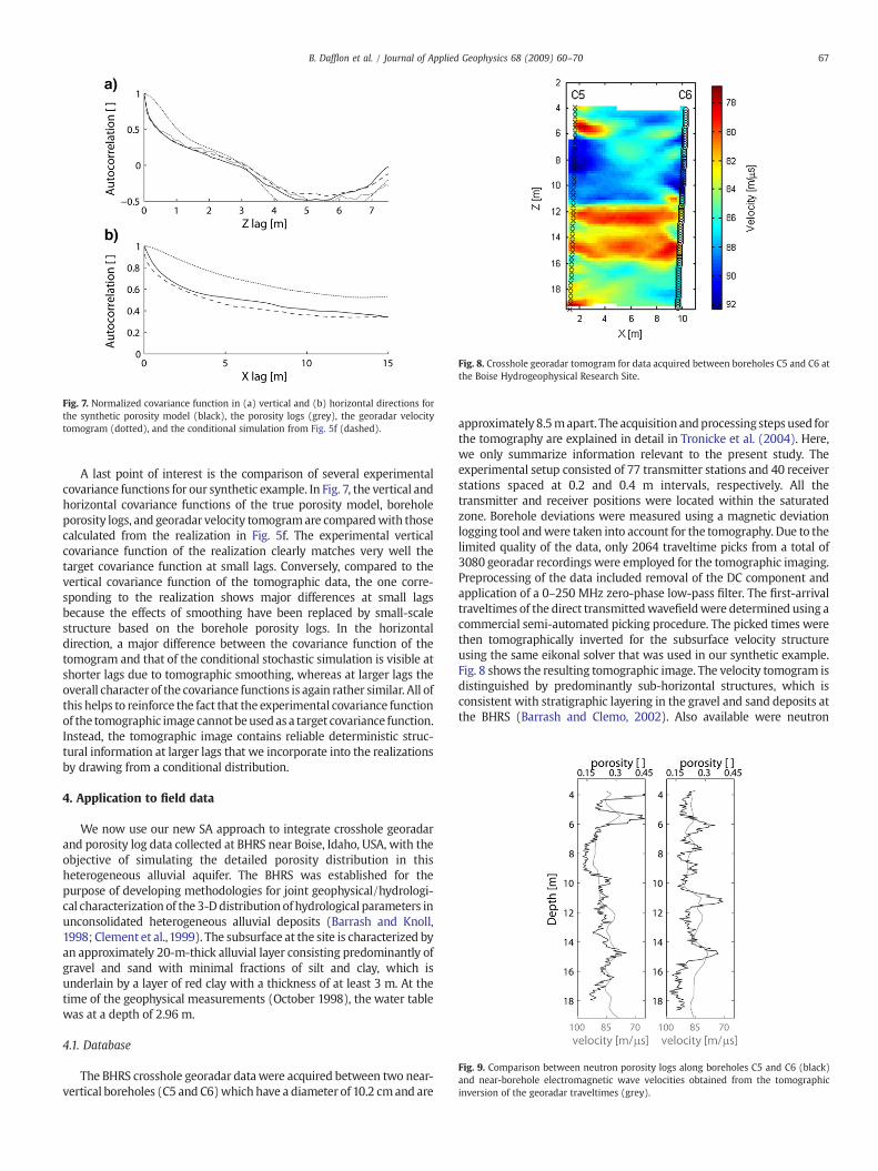
Fig. 7. Normalized covariance function in (a) vertical and (b) horizontal directions forthe synthetic porosity model (black), the porosity logs (grey), the georadar velocitytomogram (dotted), and the conditional simulation from Fig. 5f (dashed).

Fig. 8. Crosshole georadar tomogram for data acquired between boreholes C5 and C6 atthe Boise Hydrogeophysical Research Site.

Fig. 9. Comparison between neutron porosity logs along boreholes C5 and C6 (black)and near-borehole electromagnetic wave velocities obtained from the tomographicinversion of the georadar traveltimes (grey).


A last point of interest is the comparison of several experimentalcovariance functions for our synthetic example. In Fig. 7, the vertical andhorizontal covariance functions of the true porosity model, boreholeporosity logs, and georadar velocity tomogramare comparedwith thosecalculated from the realization in Fig. 5f. The experimental verticalcovariance function of the realization clearly matches very well thetarget covariance function at small lags. Conversely, compared to thevertical covariance function of the tomographic data, the one corre-sponding to the realization shows major differences at small lagsbecause the effects of smoothing have been replaced by small-scalestructure based on the borehole porosity logs. In the horizontaldirection, a major difference between the covariance function of thetomogram and that of the conditional stochastic simulation is visible atshorter lags due to tomographic smoothing, whereas at larger lags theoverall character of the covariance functions is again rather similar. All ofthis helps to reinforce the fact that the experimental covariance functionof the tomographic image cannotbeusedasa target covariance function.Instead, the tomographic image contains reliable deterministic struc-tural information at larger lags that we incorporate into the realizationsby drawing from a conditional distribution.

4. Application to field data

We now use our new SA approach to integrate crosshole georadarand porosity log data collected at BHRS near Boise, Idaho, USA, with theobjective of simulating the detailed porosity distribution in thisheterogeneous alluvial aquifer. The BHRS was established for thepurpose of developing methodologies for joint geophysical/hydrologi-cal characterization of the 3-Ddistribution of hydrological parameters inunconsolidated heterogeneous alluvial deposits (Barrash and Knoll,1998; Clement et al.,1999). The subsurface at the site is characterized byan approximately 20-m-thick alluvial layer consisting predominantly ofgravel and sand with minimal fractions of silt and clay, which isunderlain by a layer of red clay with a thickness of at least 3 m. At thetime of the geophysical measurements (October 1998), the water tablewas at a depth of 2.96 m.

4.1. Database

The BHRS crosshole georadar datawere acquired between two near-vertical boreholes (C5 and C6)which have a diameter of 10.2 cmand are

approximately 8.5mapart. The acquisition andprocessing steps used forthe tomography are explained in detail in Tronicke et al. (2004). Here,we only summarize information relevant to the present study. Theexperimental setup consisted of 77 transmitter stations and 40 receiverstations spaced at 0.2 and 0.4 m intervals, respectively. All thetransmitter and receiver positions were located within the saturatedzone. Borehole deviations were measured using a magnetic deviationlogging tool andwere taken into account for the tomography. Due to thelimited quality of the data, only 2064 traveltime picks from a total of3080 georadar recordings were employed for the tomographic imaging.Preprocessing of the data included removal of the DC component andapplication of a 0–250 MHz zero-phase low-pass filter. The first-arrivaltraveltimes of the direct transmittedwavefieldwere determined using acommercial semi-automated picking procedure. The picked times werethen tomographically inverted for the subsurface velocity structureusing the same eikonal solver that was used in our synthetic example.Fig. 8 shows the resulting tomographic image. The velocity tomogram isdistinguished by predominantly sub-horizontal structures, which isconsistent with stratigraphic layering in the gravel and sand deposits atthe BHRS (Barrash and Clemo, 2002). Also available were neutron


porosity log data, which were measured in boreholes C5 and C6 every0.06 m (Barrash and Clemo, 2002).

4.2. Conditional simulation

As in the synthetic example, our first step towards integrating theavailable BHRS georadar and porosity log data was to estimate theconditional distribution of porosity given these data. Fig. 9 shows theporosity at each borehole location and the crosshole georadar velocityadjacent to theboreholes, plotted as a functionof depth. As expected, theprominent variations in the porosity logs are also present in thetomograms along the boreholes, whereas the more subtle variationshave generally no expression in the tomographic data. The averagecorrelation coefficient between the georadar velocities and the neutronporosity logs is −0.51, whereas calculated independently along bore-holes C5 and C6 the correlation coefficients are −0.61 and −0.36,respectively. Although the correlation between georadar velocity andporosity inborehole C6 is relatively lowandwill increase theuncertaintyin the inferred conditional relationship between these parameters(compared to our synthetic example), these data still offer usefulinformation. A possible explanation for the fact that the correlationalong borehole C6 is worse than along borehole C5 could be thatstructural disturbances introduced during the drilling process are moresevere for C6 than for C5. Such local disturbances in the immediatevicinity of the boreholesmayhave a significant influence on the porositylog data, but are unlikely to be reflected in the crosshole tomogram.

Fig.10 shows a scatter plot of the velocity and porosity data from Fig. 9,where thedata frombothboreholes havebeenpooled together. Looking atthisfigure,wemakeagain theassumption that theconditional expectationcan be expressed as a linear relation. However, to capture the variabilityabout the mean trend seen in Fig. 10, we assume that the conditionalrelationship between velocity and porosity is best described by a log-normal distribution. This decision was based on the analysis of porosityresiduals about the best-fit line, aswell as examination of the histogramoftheporosity logdata (Fig.12),which showsa log-normal-typedistributioninstead of the normal-type distribution seen in Fig. 6. From the data weobtain E(ϕ|c)=−9.41e−3×c+1.04 and σ(ϕ|c)=0.058 for the condi-tional expectation and standard deviation. To generate the startingmodeland for each perturbation in the SA procedure, values are drawn from thisconditional log-normal distribution for every subsurface location except atthe boreholes. Again, the distribution of porosity at the boreholes is moretightly constrained by the neutron porosity logs, andwe thus draw from aconditional distributionwith expectation given by the porosity values andstandard deviation σ=0.005.

Fig. 10. Scatter plot of the BHRS near-borehole georadar velocity versus porosity data(for both boreholes). The conditional expectation E(ϕ|c), estimated assuming a linearrelationship and minimizing the squared error, is indicated by the straight line. Thecurved lines show the shape of the log-normal conditional distribution for porositygiven some value of georadar velocity.

Next, we must define a geostatistical model for the porosity distri-bution to fill in the small-scale information missing in the tomographydata. For the vertical target covariance function, we again used a vonKármánparametricmodel fitted to the porosity log data at short lags. Thismodel is characterized bya correlation length of 1.5mandaν-value of 0.2,andwas not varied in the simulations. Following the same reasoning as inour synthetic example, we constrained the realizations to this verticalparametric model at lags smaller than 2 m. For the horizontal targetcovariance function, we used a ν-value of 0.2 and fixed the limit ofconsidered lags to 5 m. Here, only the horizontal correlation length wasvaried in the simulations.

4.3. Results

Fig. 11 shows realizations obtained with our SA conditionalsimulation method using horizontal correlation lengths of 10, 15, 20and 30 m, respectively, which are between 6 and 20 times larger thanthe vertical correlation length of 1.5 m. As in the synthetic case, noticethat the lateral continuity increases with the horizontal correlationlength, but only at scales below the cut-off lengthwhere the realizationswere constrained to the covariance model. The general structure of theconditional simulations is also consistent with information regardingthe true structure of the BHRS aquifer. In particular, we have thepresence of three major geological units in depth having low, high, andmedium porosity, respectively. In addition, all of the results show astriking degree of structural resemblance with a recently publishedtime-domain full-waveform inversion of the crosshole radar datawhichhas an expected resolution of less than half a meter in both the verticaland horizontal directions (Ernst et al., 2007). Based on this comparison,it appears that the models characterized by intermediate correlationlengths are likely to be more realistic than those characterized by theend-members of the considered range. Albeit circumstantial, thisevidence is consistent with information on the average ratio of thehorizontal to vertical correlation length in alluvial aquifers compiled byGelhar (1993). Moreover, it is important to note that the overallhistograms of the modeled porosity structures are clearly of log-normalcharacter and indeed compare very favorably with the histogram of theporosity logs (Fig.12). The somewhat stronger presence of high porosityvalues in the stochastic realizations compared to the porosity logs couldbe the result of an incomplete representation of the borehole logs and/or a small overestimation of porosity due to the limited informationavailable to constrain the conditional distribution inferred from thegeoradar tomography. On one hand, very high porosities of 50% havebeen reported at the BHRS (Barrash and Clemo, 2002). On the otherhand, the available information limits the perfect characterization of thedifferent units. It is conceivable that with more information regardingeach of the three principal units and their distribution, more specificrelationships could be used to characterize each unit separately, as forexample the use ofmodal distribution or clusteringmethods (Hyndmanet al., 1994; Tronicke et al., 2004; Linde et al., 2006; Paasche et al., 2006)to define the conditional distribution of porositygivengeoradar velocity.

5. Conclusions

The main objective of this study was to develop a conditionalstochastic simulation method that allows for the effective, quantitativeintegration of high-resolution geophysical data. We have developed anovel SA-based approach that demonstrates strong potential forgenerating highly detailed and realistic aquifer models honoringdifferent data and prior information. Amajor advantage of our approachcomparedwith related previous efforts is that deterministic informationwith regard to the larger-scale subsurface structure, as provided, forexample, by tomographic geophysical images, is more thoroughly andappropriately incorporated into the resulting realizations. An additionaladvantage of this approach is that, because of a dramatically simplifiedglobal objective function, our algorithm exhibits very favorable

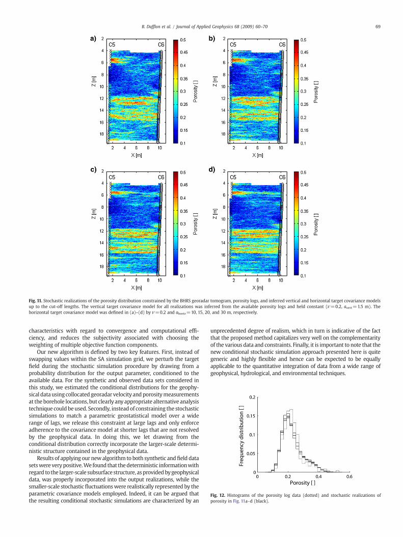
Fig. 11. Stochastic realizations of the porosity distribution constrained by the BHRS georadar tomogram, porosity logs, and inferred vertical and horizontal target covariance modelsup to the cut-off lengths. The vertical target covariance model for all realizations was inferred from the available porosity logs and held constant (ν=0.2, avert=1.5 m). Thehorizontal target covariance model was defined in (a)–(d) by ν=0.2 and ahoriz=10, 15, 20, and 30 m, respectively.

Fig. 12. Histograms of the porosity log data (dotted) and stochastic realizations ofporosity in Fig. 11a–d (black).


characteristics with regard to convergence and computational effi-ciency, and reduces the subjectivity associated with choosing theweighting of multiple objective function components.

Our new algorithm is defined by two key features. First, instead ofswapping values within the SA simulation grid, we perturb the targetfield during the stochastic simulation procedure by drawing from aprobability distribution for the output parameter, conditioned to theavailable data. For the synthetic and observed data sets considered inthis study, we estimated the conditional distributions for the geophy-sical data using collocated georadarvelocity andporositymeasurementsat the borehole locations, but clearly anyappropriate alternative analysistechnique couldbeused. Secondly, insteadof constraining the stochasticsimulations to match a parametric geostatistical model over a widerange of lags, we release this constraint at large lags and only enforceadherence to the covariance model at shorter lags that are not resolvedby the geophysical data. In doing this, we let drawing from theconditional distribution correctly incorporate the larger-scale determi-nistic structure contained in the geophysical data.

Results of applying our newalgorithm to both synthetic andfield datasetswere verypositive.We found that thedeterministic informationwithregard to the larger-scale subsurface structure, asprovidedbygeophysicaldata, was properly incorporated into the output realizations, while thesmaller-scale stochastic fluctuationswere realistically represented by theparametric covariance models employed. Indeed, it can be argued thatthe resulting conditional stochastic simulations are characterized by an

unprecedented degree of realism, which in turn is indicative of the factthat the proposed method capitalizes very well on the complementarityof the various data and constraints. Finally, it is important to note that thenew conditional stochastic simulation approach presented here is quitegeneric and highly flexible and hence can be expected to be equallyapplicable to the quantitative integration of data from a wide range ofgeophysical, hydrological, and environmental techniques.


Acknowledgments

This researchwas supported bya grant from theSwissNational Fund.We thank CGISS at Boise State University for granting us the permissiontoworkwith crosshole georadar and neutronporosity log data collectedat theBHRS.Wealso thank JensTronickeat theUniversity of Potsdamforhelpful comments and suggestions and access to the results of previouswork, as well as the two anonymous reviewers whose suggestionsgreatly improved this manuscript.

References

Avseth, P.,Mukerji, T., Jorstad, A.,Mavko, G., Veggeland, T., 2001. Seismic reservoirmappingfrom 3-D AVO in a North Sea turbidite system. Geophysics 66 (4), 1157–1176.

Bachrach, R., 2006. Joint estimation of porosity and saturation using stochastic rock-physics modeling. Geophysics 71 (5), O53–O63.

Barrash, W., Clemo, T., 2002. Hierarchical geostatistics and multifacies systems: BoiseHydrogeophysical Research Site, Boise, Idaho. Water Resources Research 38 (10).

Barrash, W., Knoll, M.D., 1998. Design of Research Wellfield for Calibrating GeophysicalMethods Against Hydrologic Parameter, Conference on Hazardous Waste Research,Great Plains/Rocky Mountains Hazardous Substance Research Center, Snowbird,UT.

Bosch, M., 1999. Lithologic tomography: from plural geophysical data to lithologyestimation. Journal of Geophysical Research-Solid Earth 104 (B1), 749–766.

Caers, J., Avseth, P., Mukerji, T., 2001. Geostatistical integration of rock physics, seismicamplitudes, and geologic models in North Sea turbidite systems. The Leading Edge20 (3), 308–312.

Chen, J.S., Hubbard, S., Rubin, Y., 2001. Estimating the hydraulic conductivity at the SouthOyster Site from geophysical tomographic data using Bayesian techniques based onthe normal linear regression model. Water Resources Research 37 (6), 1603–1613.

Clement,W.P., Knoll, M.D., Liberty, L.M., Donaldson, P.R., Michaels, P., Barrash,W., Pelton,J.R., 1999. Geophysical Surveys across the Boise Hydrogeophysical Research Site toDetermineGeophysical Parameters of a Shallow, Alluvial Aquifer, Symposiumon theApplication of Geophysics to Engineering and Environmental Problems(SAGEEP99). Environmental and Engineering Geophysical Society, Oakland, CA.

Davis, J.L., Annan, A.P., 1989. Ground-penetrating radar for high-resolution mapping ofsoil and rock stratigraphy. Geophysical Prospecting 37 (5), 531–551.

Day-Lewis, F.D., Lane, J.W., 2004. Assessing the resolution-dependent utility oftomograms for geostatistics. Geophysical Research Letters 31 (7).

Day-Lewis, F.D., Singha, K., Binley, A.M., 2005. Applying petrophysical models to radartravel time and electrical resistivity tomograms: resolution-dependent limitations.Journal of Geophysical Research-Solid Earth 110 (B8).

Desbarats, A.J., Bachu, S., 1994. Geostatistical analysis of aquifer heterogeneity from thecore scale to the basin-scale—a case-study.Water Resources Research30 (3), 673–684.

Deutsch, C.V., 2002. Geostatistical Reservoir Modeling. Oxford Univ. Press, New York.Deutsch, C.V., Wen, X.H., 1998. An improved perturbation mechanism for simulated

annealing simulation. Mathematical Geology 30 (7), 801–816.Deutsch, C.V., Wen, X.H., 2000. Integrating large-scale soft data by simulated annealing

and probability constraints. Mathematical Geology 32 (1), 49–67.Ernst, J.R., Maurer, H., Green, A.G., Holliger, K., 2007. Application of a new 2D time-

domain full-waveform inversion scheme to crosshole radar data. Geophysics 72,J53–J64.

Ezzedine, S., Rubin, Y., Chen, J.S., 1999. Bayesian method for hydrogeological sitecharacterization using borehole and geophysical survey data: theory and applica-tion to the Lawrence Livermore National Laboratory Superfund site. WaterResources Research 35 (9), 2671–2683.

Gelhar, L.W., 1993. Stochastic Subsurface Hydrology. Prentice-Hall, Englewood Cliffs.Goff, J.A., Jordan, T.H., 1988. Stochastic modeling of seafloor morphology—inversion of

sea beam data for 2nd-order statistics. Journal of Geophysical Research-Solid Earthand Planets 93 (B11), 13589–13608.

Goovaerts, P., 1997. Geostatistics for Natural Resources Evaluation. Oxford Univ. Press,New York.

Hansen, T.M., Journel, A.G., Tarantola, A., Mosegaard, K., 2006. Linear inverse Gaussiantheory and geostatistics. Geophysics 71 (6), R101–R111.

Hansen, T.M., Looms, M.C., Nielsen, L., 2008. Inferring the subsurface structuralcovariance model using cross-borehole ground penetrating radar tomography.Vadose Zone Journal 7 (1), 249–262.

Hardy, H.H., Beier, R.A., 1994. Fractals in reservoir engineering.World Scientific, Singapore.

Heinz, J., Kleineidam, S., Teutsch, G., Aigner, T., 2003. Heterogeneity patterns ofQuaternary glaciofluvial gravel bodies (SW-Germany): application to hydrogeol-ogy. Sedimentary Geology 158 (1–2), 1–23.

Holliger, K., Bergmann, T., 2002. Numerical modeling of borehole georadar data.Geophysics 67 (4), 1249–1257.

Holliger, K., Goff, J.A., 2003. A generalised model for the 1/f-scaling nature of seismicvelocity fluctuations. In: Goff, J.A., Holliger, K. (Eds.), Heterogeneity in the Crust andUpper Mantle—Nature, Scaling, and Seismic Properties. Kluwer Academic/PlenumScientific Publishers, pp. 131–154.

Hubbard, S.S., Chen, J.S., Peterson, J., Majer, E.L., Williams, K.H., Swift, D.J., Mailloux, B.,Rubin, Y., 2001. Hydrogeological characterization of the South Oyster BacterialTransport Site using geophysical data. Water Resources Research 37 (10), 2431–2456.

Hubbard, S.S., Rubin, Y., 2005. Hydrogeophysics. In: Rubin, Y., Hubbard, S.S. (Eds.),Hydrogeophysics. Springer.

Hyndman, D.W., Harris, J.M., Gorelick, S.M., 1994. Coupled seismic and tracer testinversion for aquifer property characterization. Water Resources Research 30 (7),1965–1977.

Hyndman, D.W., Harris, J.M., Gorelick, S.M., 2000. Inferring the relation between seismicslowness and hydraulic conductivity in heterogeneous aquifers. Water ResourcesResearch 36 (8), 2121–2132.

Kelkar, M., Perez, G., 2002. Applied Geostatistics for Reservoir Characterization. Societyof Petroleum engineers.

Kowalsky, M.B., Finsterle, S., Peterson, J., Hubbard, S., Rubin, Y., Majer, E., Ward, A., Gee,G., 2005. Estimation of field-scale soil hydraulic and dielectric parameters throughjoint inversion of GPR and hydrological data. Water Resources Research 41 (11).

Lanz, E., Maurer, H., Green, A.G., 1998. Refraction tomography over a buried wastedisposal site. Geophysics 63 (4), 1414–1433.

Linde, N., Finsterle, S., Hubbard, S., 2006. Inversion of tracer test data using tomographicconstraints. Water Resources Research 42 (4).

McKenna, S.A., Poeter, E.P., 1995. Field example of data fusion in site characterization.Water Resources Research 31 (12), 3229–3240.

Moysey, S., Singha, K., Knight, R., 2005. A framework for inferring field-scale rock physicsrelationships through numerical simulation. Geophysical Research Letters 32 (8).

Mukerji, T., Jorstad, A., Avseth, P., Mavko, G., Granli, J.R., 2001. Mapping lithofacies andpore-fluid probabilities in a North Sea reservoir: Seismic inversions and statisticalrock physics. Geophysics 66 (4), 988–1001.

Ortiz, C.J., Deutsch, C.V., 2002. Calculation of uncertainty in the variogram. Mathema-tical Geology 34 (2), 169–183.

Paasche, H., Tronicke, J., Holliger, K., Green, A.G., Maurer, H., 2006. Integration of diversephysical-property models: subsurface zonation and petrophysical parameterestimation based on fuzzy c-means cluster analyses. Geophysics 71 (3), H33–H44.

Parks, K.P., Bentley, L.R., Crowe, A.S., 2000. Capturing geological realism in stochasticsimulations of rock systems with Markov statistics and simulated annealing.Journal of Sedimentary Research 70 (4), 803–813.

Ramirez, A.L., Nitao, J.J., Hanley, W.G., Aines, R., Glaser, R.E., Sengupta, S.K., Dyer, K.M.,Hickling, T.L., Daily, W.D., 2005. Stochastic inversion of electrical resistivity changesusing a Markov Chain Monte Carlo approach. Journal of Geophysical Research-SolidEarth 110 (B2).

Schön, J.H., 1998. Physical Properties of Rocks: Fundamentals and Principles of Petrophysics:.Pergamon Press, Inc.

Sudicky, E.A., Huyakorn, P.S., 1991. Contaminant migration in imperfectly knownheterogeneous groundwater systems. Reviews of Geophysics 29, 240–253.

Tronicke, J., Dietrich, P., Wahlig, U., Appel, E., 2002. Integrating surface georadar andcrosshole radar tomography: a validation experiment in braided stream deposits.Geophysics 67 (5), 1516–1523.

Tronicke, J., Holliger, K., 2005. Quantitative integration of hydrogeophysical data:conditional geostatistical simulation for characterizing heterogeneous alluvialaquifers. Geophysics 70 (3), H1–H10.

Tronicke, J., Holliger, K., Barrash, W., Knoll, M.D., 2004. Multivariate analysis of cross-hole georadar velocity and attenuation tomograms for aquifer zonation. WaterResources Research 40 (1).

von Kármán, T., 1948. Progress in the statistical theory of turbulence. Maritime ResearchJournal 7, 252–264.

Walden, A.T., Hosken, J.W.J., 1985. An investigation of the spectral properties of primaryreflection coefficients. Geophysical Prospecting 33 (3), 400–435.

Williamson, P.R., Worthington, M.H., 1993. Resolution limits in ray tomography due towave behavior—numerical experiments. Geophysics 58 (5), 727–735.

Zheng, C.M., Gorelick, S.M., 2003. Analysis of solute transport in flow fields influencedby preferential flowpaths at the decimeter scale. Ground Water 41 (2), 142–155.

simulated-annealing-based conditional simulation for the

Documents