Simple Useful Flow Configurations …

P M V SubbaraoProfessor

Mechanical Engineering Department

I I T Delhi

Exact Solutions of NS Equations

The Curl of Stokes Flow Equation

Taking the curl of Stokes flow equation:

pv 2

pv 2

pvv

Using the vector identity vvv 2

With 0 v

pv

0

Stokes' Solution for an Immersed Sphere

Strokes defined a stream function in spherical coordinate system (1851) as:

sin

12r

vr rrv

sin

1

0

sin

sin

11 2

2

v

rr

vr

rr

A solenoid condition in spherical coordinate system

e

rre

rv r

sin

1

sin

12

e

rre

rv r

sin

1

sin

12 v

sin

1sin

sin 22

2

rrr

e

0

the momentum equation as a scalar equation for ψ.

0sin

1sin

sin 22

2

rrr

e

0sin

1sin2

22

2

rr

0cot1

2

22

2

22

2

rrr

The boundary conditions

The problem appears formidable, but in fact it yields readily to a product solution (r, ) = f(r)g().

2sin, rfr

F(r) is governed by the equi-dimensional differential equation:

0cot1

2

22

2

22

2

rrr

02

2

22

2

f

rdr

d

whose solutions are of the form f(r) r∝ n, It is easy to verify that n = −1, 1, 2,4 so that

42 DrCrBrr

Arf

422sin, DrCrBr

r

Ar

The boundary conditions

2

222 23

sin4

1,

a

r

a

r

r

aUar

Inside the parentheses, the first term corresponds to the uniform flow. and the second term to the doublet; together they represent an inviscid flow past a sphere. The third term is called the Stokeslet, representing the viscous correction.

2

222 23

sin4

1,

a

r

a

r

r

aUar

The velocity components follow immediately

r

a

r

aUvr 2

3

21cos

3

3

r

a

r

aUv

4

3

41sin

3

3

Properties of Stokes Solution

• This celebrated solution has several extraordinary properties:

• 1. The streamlines and velocities are entirely independent of the fluid viscosity.

• This is true of all creeping flows.

• 2. The streamlines possess perfect fore-and-aft symmetry.

• There is no wake.

• 3. The local velocity is everywhere retarded from its freestream value.

• 4. The effect of the sphere extends to enormous distances:

• At r = 10a, the velocities are still about 10 percent below their freestream values.

Pressure Field for an Immersed Sphere

Stokes Flow Equation

er

a

r

aUe

r

a

r

aUv r

4

3

41sin

2

3

21cos

3

3

3

3

cos

3r

Ua

r

p

vvv 2 vvp

vp

Integrating with respect to r from r=a to r∞, we get

cos

2

32r

Uapp

where p, is the uniform freestream pressure. The pressure deviation is proportional to and antisymmetric. Positive at the front and negative at the rear of the sphere

pv 2 With 0 v

This creates a pressure drag on the sphere.

Stress Field

• There is a surface shear stress which creates a drag force.

• The shear-stress distribution in the fluid is given by

Stokes Drag on Sphere

• The total drag is found by integrating pressure and shear around the surface:

This is the famous sphere-drag formula of Stokes (1851).Consists of two-thirds viscous force and one-third pressure force. The formula is strictly valid only for Re << 1 but agrees with experiment up to about Re = 1.

Other Three-Dimensional Body Shapes

• In principle, a Stokes flow analysis is possible for any three-dimensional body shape, providing that one has the necessary analytical skill.

• A number of interesting shapes are discussed in the literature.

• Of particular interest is the drag of a circular disk:

Disk normal to the freestream:

Disk parallel to the freestream:

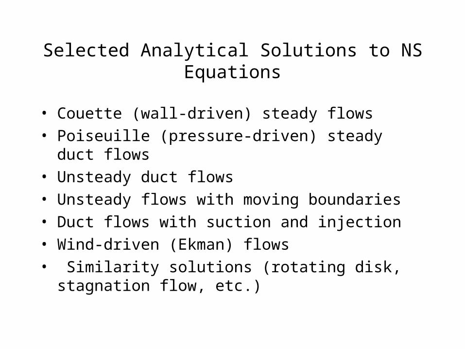
Selected Analytical Solutions to NS Equations

• Couette (wall-driven) steady flows

• Poiseuille (pressure-driven) steady duct flows

• Unsteady duct flows

• Unsteady flows with moving boundaries

• Duct flows with suction and injection

• Wind-driven (Ekman) flows

• Similarity solutions (rotating disk, stagnation flow, etc.)

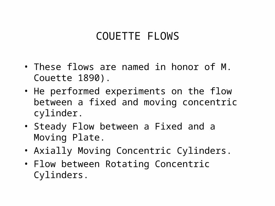
COUETTE FLOWS

• These flows are named in honor of M. Couette 1890).

• He performed experiments on the flow between a fixed and moving concentric cylinder.

• Steady Flow between a Fixed and a Moving Plate.

• Axially Moving Concentric Cylinders.

• Flow between Rotating Concentric Cylinders.

Steady Flow between a Fixed and a Moving Plate

• In above Figure two infinite plates are 2h apart, and the upper plate moves at speed U relative to the lower.

• The pressure is assumed constant.

• These boundary conditions are independent of x or z ("infinite plates");

• It follows that u = u(y) and NS equations reduce to

Continuity Equation: 0

x

u

NS Equations: 02

2

x

ud

where continuity merely verifies our assumption that u = u(y) only. NS Equation can be integrated twice to obtain

21 cycu

The boundary conditions are no slip, u(-h) = 0 and u(+h) = U. c1= U/2h and c2 = U/2.

Then the velocity distribution is

22

Uy

h

Uu y

Uu 1

2

The shear stress at any point in the flow

From the viscosity law:

x

v

y

u

y

u constanth

U yU

u 12

For the couette flow the shear stress is constant throughout the fluid. The strain rate-even a nonnewtonian fluid would maintain a linear velocity profile.

Friction coefficient

The dimensionless shear stress is usually defined in engineering flows as the friction coefficient

22

21

21 U

yu

UC f

hf Uh

CRe

1

The No-Slip Boundary Condition in Viscous Flows

• The Riddle of Fluid Sticking to the Wall in Flow.

• Consider an isolated fluid particle.

• When the particle hits a wall of a solid body, its velocity abruptly changes.

Φi

ui

iv

vi

Φrrv

ur

vr

This abrupt change in momentum of the ball is achieved by an equal and opposite change in that of

the wall or the body.

Video of the Event

• At the point of collision we can identify normal and tangential directions nˆ and tˆto the wall.

• The time of impact t0 is very brief.

• It is a good assumption to conclude that the normal velocity vn will be reversed with a reduction in magnitude because of loss of mechanical energy.

• If we assume the time of impact to be zero, the normal velocity component vn is seen to be discontinuous and also with a change in sign.

Time variation of normal and tangential velocitycomponents of the impinging particle.

Whether it is discontinuous or not, the fact that it has to change sign is obvious, since the ball cannot continue penetrating

the solid wall.

The Tangential Component of Velocity

• The case of the tangential component vt is far more complex and more interesting.

• First of all, the particle will continue to move in the same direction and hence there is no change in sign.

• If the wall and the ball are perfectly smooth (i.e. frictionless).

• vt will not change at all.

• In case of rough surfaces vt will decrease a little.

• It is important to note that vt is nowhere zero.

• Even though the ball sticks to the wall for a brief period t0, at no time its tangential velocity is zero!

• The ball can also roll on the wall.