Similarity of Objects and the Meaning of Words?

Rudi Cilibrasi and Paul Vitanyi??

CWI, Kruislaan 413, 1098 SJ Amsterdam,The Netherlands. Email: Rudi.Cilibrasi@cwi.nl; Paul.Vitanyi@cwi.nl

Abstract. We survey the emerging area of compression-based, parameter-free,similarity distance measures useful in data-mining, pattern recognition, learningand automatic semantics extraction. Given a family of distances on a set of ob-jects, a distance is universal up to a certain precision for that family if it minorizesevery distance in the family between every two objects in the set, up to the statedprecision (we do not require the universal distance to be an element of the fam-ily). We consider similarity distances for two types of objects: literal objects thatas such contain all of their meaning, like genomes or books, and names for ob-jects. The latter may have literal embodyments like the first type, but may alsobe abstract like “red” or “christianity.” For the first type we consider a family ofcomputable distance measures corresponding to parameters expressing similarityaccording to particular features between pairs of literal objects. For the secondtype we consider similarity distances generated by web users corresponding toparticular semantic relations between the (names for) the designated objects. Forboth families we give universal similarity distance measures, incorporating allparticular distance measures in the family. In the first case the universal distanceis based on compression and in the second case it is based on Google page countsrelated to search terms. In both cases experiments on a massive scale give evi-dence of the viability of the approaches.

1 Introduction

Objects can be given literally, like the literal four-letter genome of a mouse, or theliteral text of War and Peace by Tolstoy. For simplicity we take it that all meaning ofthe object is represented by the literal object itself. Objects can also be given by name,like “the four-letter genome of a mouse,” or “the text of War and Peace by Tolstoy.”There are also objects that cannot be given literally, but only by name and acquire theirmeaning from their contexts in background common knowledge in humankind, like“home” or “red.” In the literal setting, objective similarity of objects can be establishedby feature analysis, one type of similarity per feature. In the abstract “name” setting,all similarity must depend on background knowledge and common semantics relations,which is inherently subjective and “in the mind of the beholder.”

? This work supported in part by the EU sixth framework project RESQ, IST–1999–11234, theNoE QUIPROCONE IST–1999–29064, the ESF QiT Programmme, and the EU NoE PASCAL,and by the Netherlands Organization for Scientific Research (NWO) under Grant 612.052.004.

?? Also affiliated with the Computer Science Department, University of Amsterdam.

1.1 Compression Based Similarity

All data are created equal but some data are more alike than others. We and othershave recently proposed very general methods expressing this alikeness, using a newsimilarity metric based on compression. It is parameter-free in that it doesn’t use anyfeatures or background knowledge about the data, and can without changes be appliedto different areas and across area boundaries. Put differently: just like ‘parameter-free’statistical methods, the new method uses essentially unboundedly many parameters, theones that are appropriate. It is universal in that it approximates the parameter expressingsimilarity of the dominant feature in all pairwise comparisons. It is robust in the sensethat its success appears independent from the type of compressor used. The clusteringwe use is hierarchical clustering in dendrograms based on a new fast heuristic for thequartet method. The method is available as an open-source software tool, [7].

Feature-Based Similarities: We are presented with unknown data and the questionis to determine the similarities among them and group like with like together. Com-monly, the data are of a certain type: music files, transaction records of ATM machines,credit card applications, genomic data. In these data there are hidden relations that wewould like to get out in the open. For example, from genomic data one can extract letter-or block frequencies (the blocks are over the four-letter alphabet); from music files onecan extract various specific numerical features, related to pitch, rhythm, harmony etc.One can extract such features using for instance Fourier transforms [39] or wavelettransforms [18], to quantify parameters expressing similarity. The resulting vectors cor-responding to the various files are then classified or clustered using existing classifica-tion software, based on various standard statistical pattern recognition classifiers [39],Bayesian classifiers [15], hidden Markov models [9], ensembles of nearest-neighborclassifiers [18] or neural networks [15, 34]. For example, in music one feature would beto look for rhythm in the sense of beats per minute. One can make a histogram whereeach histogram bin corresponds to a particular tempo in beats-per-minute and the as-sociated peak shows how frequent and strong that particular periodicity was over theentire piece. In [39] we see a gradual change from a few high peaks to many low andspread-out ones going from hip-hip, rock, jazz, to classical. One can use this similaritytype to try to cluster pieces in these categories. However, such a method requires spe-cific and detailed knowledge of the problem area, since one needs to know what featuresto look for.

Non-Feature Similarities: Our aim is to capture, in a single similarity metric, ev-ery effective distance: effective versions of Hamming distance, Euclidean distance, editdistances, alignment distance, Lempel-Ziv distance, and so on. This metric should be sogeneral that it works in every domain: music, text, literature, programs, genomes, exe-cutables, natural language determination, equally and simultaneously. It would be ableto simultaneously detect all similarities between pieces that other effective distancescan detect seperately.

The normalized version of the “information metric” of [32, 3] fills the requirementsfor such a “universal” metric. Roughly speaking, two objects are deemed close if we cansignificantly “compress” one given the information in the other, the idea being that iftwo pieces are more similar, then we can more succinctly describe one given the other.The mathematics used is based on Kolmogorov complexity theory [32].

1.2 A Brief History

In view of the success of the method, in numerous applications, it is perhaps useful totrace its descent in some detail. Let K(x) denote the unconditional Kolmogorov com-plexity of x, and let K(x|y) denote the conditional Kolmogorov complexity of x giveny. Intuitively, the Kolmorov complexity of an object is the number of bits in the ul-timate compressed version of the object, or, more precisely, from which the objectcan be recovered by a fixed algorithm. The “sum” version of information distance,K(x|y)+ K(y|x), arose from thermodynamical considerations about reversible compu-tations [25, 26] in 1992. It is a metric and minorizes all computable distances satisfyinga given density condition up to a multiplicative factor of 2. Subsequently, in 1993, the“max” version of information distance, maxK(x|y),K(y|x), was introduced in [3].Up to a logarithmic additive term, it is the length of the shortest binary program thattransforms x into y, and y into x. It is a metric as well, and this metric minorizes allcomputable distances satisfying a given density condition up to an additive ignorableterm. This is optimal. But the Kolmogorov complexity is uncomputable, which seems topreclude application altogether. However, in 1999 the normalized version of the “sum”information distance (K(x|y)+ K(y|x))/K(xy) was introduced as a similarity distanceand applied to construct a phylogeny of bacteria in [28], and subsequently mammalphylogeny in 2001 [29], followed by plagiarism detection in student programming as-signments [6], and phylogeny of chain letters in [4]. In [29] it was shown that the nor-malized sum distance is a metric, and minorizes certain computable distances up toa multiplicative factor of 2 with high probability. In a bold move, in these papers theuncomputable Kolmogorov complexity was replaced by an approximation using a real-world compressor, for example the special-purpose genome compressor GenCompress.Note that, because of the uncomputability of the Kolmogorov complexity, in principleone cannot determine the degree of accuracy of the approximation to the target value.Yet it turned out that this practical approximation, imprecise though it is, but guided byan ideal provable theory, in general gives good results on natural data sets. The early useof the “sum” distance was replaced by the “max” distance in [30] in 2001 and applied tomammal phylogeny in 2001 in the early version of [31] and in later versions also to thelanguage tree. In [31] it was shown that an appropriately normalized “max” distance ismetric, and minorizes all normalized computable distances satisfying a certain densityproperty up to an additive vanishing term. That is, it discovers all effective similaritiesof this family in the sense that if two objects are close according to some effective sim-ilarity, then they are also close according to the normalized information distance. Putdifferently, the normalized information distance represents similarity according to thedominating shared feature between the two objects being compared. In comparisons ofmore than two objects, different pairs may have different dominating features. For everytwo objects, this universal metric distance zooms in on the dominant similarity betweenthose two objects out of a wide class of admissible similarity features. Hence it maybe called “the” similarity metric. In 2003 [12] it was realized that the method could beused for hierarchical clustering of natural data sets from arbitrary (also heterogenous)domains, and the theory related to the application of real-world compressors was devel-oped, and numerous applications in different domains were given, Section 3. In [19] theauthors use a simplified version of the similarity metric, which also performs well. In

[2], and follow-up work, a closely related notion of compression-based distances is pro-posed. There the purpose was initially to infer a language tree from different-languagetext corpora, as well as do authorship attribution on basis of text corpora. The distancesdetermined between objects are justified by ad-hoc plausibility arguments and representa partially independent development (although they refer to the information distance ap-proach of [27, 3]). Altogether, it appears that the notion of compression-based similaritymetric is so powerful that its performance is robust under considerable variations.

2 Similarity Distance

We briefly outline an improved version of the main theoretical contents of [12] andits relation to [31]. For details and proofs see these references. First, we give a preciseformal meaning to the loose distance notion of “degree of similarity” used in the patternrecognition literature.

2.1 Distance and Metric

Let Ω be a nonempty set and R + be the set of nonnegative real numbers. A distancefunction on Ω is a function D : Ω×Ω → R +. It is a metric if it satisfies the metric(in)equalities:

– D(x,y) = 0 iff x = y,– D(x,y) = D(y,x) (symmetry), and– D(x,y) ≤ D(x,z)+D(z,y) (triangle inequality).

The value D(x,y) is called the distance between x,y ∈ Ω. A familiar example of a dis-tance that is also metric is the Euclidean metric, the everyday distance e(a,b) betweentwo geographical objects a,b expressed in, say, meters. Clearly, this distance satisfiesthe properties e(a,a) = 0, e(a,b) = e(b,a), and e(a,b) ≤ e(a,c)+ e(c,b) (for instance,a = Amsterdam, b = Brussels, and c = Chicago.) We are interested in a particulartype of distance, the “similarity distance”, which we formally define in Definition 4.For example, if the objects are classical music pieces then the function D defined byD(a,b) = 0 if a and b are by the same composer and D(a,b) = 1 otherwise, is a sim-ilarity distance that is also a metric. This metric captures only one similarity aspect(feature) of music pieces, presumably an important one that subsumes a conglomerateof more elementary features.

2.2 Admissible Distance

In defining a class of admissible distances (not necessarily metric distances) we want toexclude unrealistic ones like f (x,y) = 1

2 for every pair x 6= y. We do this by restrictingthe number of objects within a given distance of an object. As in [3] we do this by onlyconsidering effective distances, as follows.

Definition 1. Let Ω = Σ∗, with Σ a finite nonempty alphabet and Σ∗ the set of finitestrings over that alphabet. Since every finite alphabet can be recoded in binary, we

choose Σ = 0,1. In particular, “files” in computer memory are finite binary strings. Afunction D : Ω×Ω → R + is an admissible distance if for every pair of objects x,y ∈ Ωthe distance D(x,y) satisfies the density condition

∑y

2−D(x,y) ≤ 1, (1)

is computable, and is symmetric, D(x,y) = D(y,x).

If D is an admissible distance, then for every x the set D(x,y) : y ∈ 0,1∗ is thelength set of a prefix code, since it satisfies (1), the Kraft inequality. Conversely, if adistance is the length set of a prefix code, then it satisfies (1), see for example [27].

2.3 Normalized Admissible Distance

Large objects (in the sense of long strings) that differ by a tiny part are intuitively closerthan tiny objects that differ by the same amount. For example, two whole mitochondrialgenomes of 18,000 bases that differ by 9,000 are very different, while two whole nucleargenomes of 3×109 bases that differ by only 9,000 bases are very similar. Thus, absolutedifference between two objects doesn’t govern similarity, but relative difference appearsto do so.

Definition 2. A compressor is a lossless encoder mapping Ω into 0,1∗ such thatthe resulting code is a prefix code. “Lossless” means that there is a decompressor thatreconstructs the source message from the code message. For convenience of notationwe identify “compressor” with a “code word length function” C : Ω → N , where N isthe set of nonnegative integers. That is, the compressed version of a file x has lengthC(x). We only consider compressors such that C(x) ≤ |x|+ O(log |x|). (The additivelogarithmic term is due to our requirement that the compressed file be a prefix codeword.) We fix a compressor C, and call the fixed compressor the reference compressor.

Definition 3. Let D be an admissible distance. Then D+(x) is defined by D+(x) =maxD(x,z) :C(z)≤C(x), and D+(x,y) is defined by D+(x,y) = maxD+(x),D+(y).Note that since D(x,y) = D(y,x), also D+(x,y) = D+(y,x).

Definition 4. Let D be an admissible distance. The normalized admissible distance,also called a similarity distance, d(x,y), based on D relative to a reference compressorC, is defined by

d(x,y) =D(x,y)

D+(x,y).

It follows from the definitions that a normalized admissible distance is a functiond : Ω×Ω → [0,1] that is symmetric: d(x,y) = d(y,x).

Lemma 1. For every x ∈ Ω, and constant e ∈ [0,1], a normalized admissible distancesatisfies the density constraint

|y : d(x,y) ≤ e, C(y) ≤C(x)| < 2eD+(x)+1. (2)

We call a normalized distance a “similarity” distance, because it gives a relativesimilarity according to the distance (with distance 0 when objects are maximally similarand distance 1 when they are maximally dissimilar) and, conversely, for every well-defined computable notion of similarity we can express it as a metric distance accordingto our definition. In the literature a distance that expresses lack of similarity (like ours)is often called a “dissimilarity” distance or a “disparity” distance.

2.4 Normal Compressor

We give axioms determining a large family of compressors that both include most (ifnot all) real-world compressors and ensure the desired properties of the NCD to bedefined later.

Definition 5. A compressor C is normal if it satisfies, up to an additive O(logn) term,with n the maximal binary length of an element of Ω involved in the (in)equality con-cerned, the following:

1. Idempotency: C(xx) = C(x), and C(λ) = 0, where λ is the empty string.2. Monotonicity: C(xy) ≥C(x).3. Symmetry: C(xy) = C(yx).4. Distributivity: C(xy)+C(z) ≤C(xz)+C(yz).

Remark 1. These axioms are of course an idealization. The reader can insert, say O(√

n),for the O(logn) fudge term, and modify the subsequent discussion accordingly. Manycompressors, like gzip or bzip2, have a bounded window size. Since compression ofobjects exceeding the window size is not meaningful, we assume 2n is less than thewindow size. In such cases the O(logn) term, or its equivalent, relates to the fictitiousversion of the compressor where the window size can grow indefinitely. Alternatively,we bound the value of n to half te window size, and replace the fudge term O(logn) bysome small fraction of n. Other compressors, like PPMZ, have unlimited window size,and hence are more suitable for direct interpretation of the axioms.

Idempotency: A reasonable compressor will see exact repetitions and obey idem-potency up to the required precision. It will also compress the empty string to the emptystring.

Monotonicity: A real compressor must have the monotonicity property, at least upto the required precision. The property is evident for stream-based compressors, andonly slightly less evident for block-coding compressors.

Symmetry: Stream-based compressors of the Lempel-Ziv family, like gzip andpkzip, and the predictive PPM family, like PPMZ, are possibly not precisely symmet-ric. This is related to the stream-based property: the initial file x may have regularitiesto which the compressor adapts; after crossing the border to y it must unlearn thoseregularities and adapt to the ones of x. This process may cause some imprecision insymmetry that vanishes asymptotically with the length of x,y. A compressor must bepoor indeed (and will certainly not be used to any extent) if it doesn’t satisfy symmetryup to the required precision. Apart from stream-based, the other major family of com-pressors is block-coding based, like bzip2. They essentially analyze the full input block

by considering all rotations in obtaining the compressed version. It is to a great extentsymmetrical, and real experiments show no departure from symmetry.

Distributivity: The distributivity property is not immediately intuitive. In Kol-mogorov complexity theory the stronger distributivity property

C(xyz)+C(z) ≤C(xz)+C(yz) (3)

holds (with K = C). However, to prove the desired properties of NCD below, only theweaker distributivity property

C(xy)+C(z) ≤C(xz)+C(yz) (4)

above is required, also for the boundary case were C = K. In practice, real-world com-pressors appear to satisfy this weaker distributivity property up to the required precision.

Definition 6. DefineC(y|x) = C(xy)−C(x). (5)

This number C(y|x) of bits of information in y, relative to x, can be viewed as the excessnumber of bits in the compressed version of xy compared to the compressed version ofx, and is called the amount of conditional compressed information.

In the definition of compressor the decompression algorithm is not included (unlike thecase of Kolmorogov complexity, where the decompressing algorithm is given by defi-nition), but it is easy to construct one: Given the compressed version of x in C(x) bits,we can run the compressor on all candidate strings z—for example, in length-increasinglexicographical order, until we find the compressed string z0 = x. Since this string de-compresses to x we have found x = z0. Given the compressed version of xy in C(xy)bits, we repeat this process using strings xz until we find the string xz1 of which thecompressed version equals the compressed version of xy. Since the former compressedversion decompresses to xy, we have found y = z1. By the unique decompression prop-erty we find that C(y|x) is the extra number of bits we require to describe y apart fromdescribing x. It is intuitively acceptable that the conditional compressed informationC(x|y) satisfies the triangle inequality

C(x|y) ≤C(x|z)+C(z|y). (6)

Lemma 2. Both (3) and (6) imply (4).

Lemma 3. A normal compressor satisfies additionally subadditivity: C(xy) ≤ C(x)+C(y).

Subadditivity: The subadditivity property is clearly also required for every viablecompressor, since a compressor may use information acquired from x to compress y.Minor imprecision may arise from the unlearning effect of crossing the border betweenx and y, mentioned in relation to symmetry, but again this must vanish asymptoticallywith increasing length of x,y.

2.5 Normalized Information Distance

Technically, the Kolmogorov complexity of x given y is the length of the shortest binaryprogram, for the reference universal prefix Turing machine, that on input y outputsx; it is denoted as K(x|y). For precise definitions, theory and applications, see [27].The Kolmogorov complexity of x is the length of the shortest binary program withno input that outputs x; it is denoted as K(x) = K(x|λ) where λ denotes the emptyinput. Essentially, the Kolmogorov complexity of a file is the length of the ultimatecompressed version of the file. In [3] the information distance E(x,y) was introduced,defined as the length of the shortest binary program for the reference universal prefixTuring machine that, with input x computes y, and with input y computes x. It was shownthere that, up to an additive logarithmic term, E(x,y) = maxK(x|y),K(y|x). It wasshown also that E(x,y) is a metric, up to negligible violations of the metric inequalties.Moreover, it is universal in the sense that for every admissible distance D(x,y) as inDefinition 1, E(x,y) ≤ D(x,y) up to an additive constant depending on D but not onx and y. In [31], the normalized version of E(x,y), called the normalized informationdistance, is defined as

NID(x,y) =maxK(x|y),K(y|x)

maxK(x),K(y) . (7)

It too is a metric, and it is universal in the sense that this single metric minorizes up toan negligible additive error term all normalized admissible distances in the class con-sidered in [31]. Thus, if two files (of whatever type) are similar (that is, close) accordingto the particular feature described by a particular normalized admissible distance (notnecessarily metric), then they are also similar (that is, close) in the sense of the normal-ized information metric. This justifies calling the latter the similarity metric. We stressonce more that different pairs of objects may have different dominating features. Yetevery such dominant similarity is detected by the NID . However, this metric is basedon the notion of Kolmogorov complexity. Unfortunately, the Kolmogorov complexityis non-computable in the Turing sense. Approximation of the denominator of (7) by agiven compressor C is straightforward: it is maxC(x),C(y). The numerator is moretricky. It can be rewritten as

maxK(x,y)−K(x),K(x,y)−K(y), (8)

within logarithmic additive precision, by the additive property of Kolmogorov complex-ity [27]. The term K(x,y) represents the length of the shortest program for the pair (x,y).In compression practice it is easier to deal with the concatenation xy or yx. Again, withinlogarithmic precision K(x,y) = K(xy) = K(yx). Following a suggestion by Steven deRooij, one can approximate (8) best by minC(xy),C(yx)−minC(x),C(y). Here,and in the later experiments using the CompLearn Toolkit [7], we simply use C(xy)rather than minC(xy),C(yx). This is justified by the observation that block-codingbased compressors are symmetric almost by definition, and experiments with variousstream-based compressors (gzip, PPMZ) show only small deviations from symmetry.

The result of approximating the NID using a real compressor C is called the nor-malized compression distance ( NCD ), formally defined in (10). The theory as devel-oped for the Kolmogorov-complexity based NID in [31], may not hold for the (possibly

poorly) approximating NCD . It is nonetheless the case that experiments show that theNCD apparently has (some) properties that make the NID so appealing. To fill thisgap between theory and practice, we develop the theory of NCD from first principles,based on the axiomatics of Section 2.4. We show that the NCD is a quasi-universalsimilarity metric relative to a normal reference compressor C. The theory developed in[31] is the boundary case C = K, where the “quasi-universality” below has become full“universality”.

2.6 Compression Distance

We define a compression distance based on a normal compressor and show it is an ad-missible distance. In applying the approach, we have to make do with an approximationbased on a far less powerful real-world reference compressor C. A compressor C ap-proximates the information distance E(x,y), based on Kolmogorov complexity, by thecompression distance EC(x,y) defined as

EC(x,y) = C(xy)−minC(x),C(y). (9)

Here, C(xy) denotes the compressed size of the concatenation of x and y, C(x) denotesthe compressed size of x, and C(y) denotes the compressed size of y.

Lemma 4. If C is a normal compressor, then EC(x,y)+O(1) is an admissible distance.

Lemma 5. If C is a normal compressor, then EC(x,y) satisfies the metric (in)equalitiesup to logarithmic additive precision.

Lemma 6. If C is a normal compressor, then E+C (x,y) = maxC(x),C(y).

2.7 Normalized Compression Distance

The normalized version of the admissible distance EC(x,y), the compressor C based ap-proximation of the normalized information distance (7), is called the normalized com-pression distance or NCD:

NCD(x,y) =C(xy)−minC(x),C(y)

maxC(x),C(y) . (10)

This NCD is the main concept of this work. It is the real-world version of the idealnotion of normalized information distance NID in (7). Actually, the NCD is a familyof compression functions parameterized by the given data compressor C.

Remark 2. In practice, the NCD is a non-negative number 0 ≤ r ≤ 1 + ε representinghow different the two files are. Smaller numbers represent more similar files. The ε inthe upper bound is due to imperfections in our compression techniques, but for moststandard compression algorithms one is unlikely to see an ε above 0.1 (in our experi-ments gzip and bzip2 achieved NCD ’s above 1, but PPMZ always had NCD at most1).

There is a natural interpretation to NCD(x,y): If, say, C(y) ≥ C(x) then we canrewrite

NCD(x,y) =C(xy)−C(x)

C(y).

That is, the distance NCD(x,y) between x and y is the improvement due to compress-ing y using x as previously compressed “data base,” and compressing y from scratch,expressed as the ratio between the bit-wise length of the two compressed versions.Relative to the reference compressor we can define the information in x about y asC(y)−C(y|x). Then, using (5),

NCD(x,y) = 1− C(y)−C(y|x)C(y)

.

That is, the NCD between x and y is 1 minus the ratio of the information x about y andthe information in y.

Theorem 1. If the compressor is normal, then the NCD is a normalized admissibledistance satsifying the metric (in)equalities, that is, a similarity metric.

Quasi-Universality: We now digress to the theory developed in [31], which formedthe motivation for developing the NCD . If, instead of the result of some real compres-sor, we substitute the Kolmogorov complexity for the lengths of the compressed files inthe NCD formula, the result is the NID as in (7). It is universal in the following sense:Every admissible distance expressing similarity according to some feature, that can becomputed from the objects concerned, is comprised (in the sense of minorized) by theNID . Note that every feature of the data gives rise to a similarity, and, conversely, ev-ery similarity can be thought of as expressing some feature: being similar in that sense.Our actual practice in using the NCD falls short of this ideal theory in at least threerespects:

(i) The claimed universality of the NID holds only for indefinitely long sequencesx,y. Once we consider strings x,y of definite length n, it is only universal with respect to“simple” computable normalized admissible distances, where “simple” means that theyare computable by programs of length, say, logarithmic in n. This reflects the fact that,technically speaking, the universality is achieved by summing the weighted contributionof all similarity distances in the class considered with respect to the objects considered.Only similarity distances of which the complexity is small (which means that the weightis large), with respect to the size of the data concerned, kick in.

(ii) The Kolmogorov complexity is not computable, and it is in principle impossibleto compute how far off the NCD is from the NID . So we cannot in general knowhow well we are doing using the NCD of a given compressor. Rather than all “simple”distances (features, properties), like the NID , the NCD captures a subset of thesebased on the features (or combination of features) analyzed by the compressor. Fornatural data sets, however, these may well cover the features and regularities presentin the data anyway. Complex features, expressions of simple or intricate computations,like the initial segment of π = 3.1415 . . ., seem unlikely to be hidden in natural data.This fact may account for the practical success of the NCD , especially when usinggood compressors.

(iii) To approximate the NCD we use standard compression programs like gzip,PPMZ, and bzip2. While better compression of a string will always approximate theKolmogorov complexity better, this may not be true for the NCD . Due to its arithmeticform, subtraction and division, it is theoretically possible that while all items in theformula get better compressed, the improvement is not the same for all items, and theNCD value moves away from the NID value. In our experiments we have not observedthis behavior in a noticable fashion. Formally, we can state the following:

Theorem 2. Let d be a computable normalized admissible distance and C be a nor-mal compressor. Then, NCD(x,y) ≤ αd(x,y) + ε, where for C(x) ≥ C(y), we haveα = D+(x)/C(x) and ε = (C(x|y)−K(x|y))/C(x), with C(x|y) according to (5).

Remark 3. Clustering according to NCD will group sequences together that are simi-lar according to features that are not explicitly known to us. Analysis of what the com-pressor actually does, still may not tell us which features that make sense to us canbe expressed by conglomerates of features analyzed by the compressor. This can beexploited to track down unknown features implicitly in classification: forming automat-ically clusters of data and see in which cluster (if any) a new candidate is placed.

Another aspect that can be exploited is exploratory: Given that the NCD is smallfor a pair x,y of specific sequences, what does this really say about the sense in whichthese two sequences are similar? The above analysis suggests that close similarity willbe due to a dominating feature (that perhaps expresses a conglomerate of subfeatures).Looking into these deeper causes may give feedback about the appropriateness of therealized NCD distances and may help extract more intrinsic information about theobjects, than the oblivious division into clusters, by looking for the common features inthe data clusters.

2.8 Hierarchical Clustering

Given a set of objects, the pairwise NCD ’s form the entries of a distance matrix.This distance matrix contains the pairwise relations in raw form. But in this formatthat information is not easily usable. Just as the distance matrix is a reduced form ofinformation representing the original data set, we now need to reduce the informationeven further in order to achieve a cognitively acceptable format like data clusters. Thedistance matrix contains all the information in a form that is not easily usable, since forn > 3 our cognitive capabilities rapidly fail. In our situation we do not know the num-ber of clusters a-priori, and we let the data decide the clusters. The most natural way todo so is hierarchical clustering [16]. Such methods have been extensively investigatedin Computational Biology in the context of producing phylogenies of species. One themost sensitive ways is the so-called ‘quartet method. This method is sensitive, but timeconsuming, running in quartic time. Other hierarchical clustering methods, like parsi-mony, may be much faster, quadratic time, but they are less sensitive. In view of the factthat current compressors are good but limited, we want to exploit the smallest differ-ences in distances, and therefore use the most sensitive method to get greatest accuracy.Here, we use a new quartet-method (actually a new version [12] of the quartet puzzlingvariant [35]), which is a heuristic based on randomized parallel hill-climbing genetic

programming. In this paper we do not describe this method in any detail, the readeris referred to [12], or the full description in [14]. It is implemented in the CompLearnpackage [7].

We describe the idea of the algorithm, and the interpretation of the accuracy of theresulting tree representation of the data clustering. To cluster n data items, the algorithmgenerates a random ternary tree with n− 2 internal nodes and n leaves. The algorithmtries to improve the solution at each step by interchanging sub-trees rooted at internalnodes (possibly leaves). It switches if the total tree cost is improved. To find the opti-mal tree is NP-hard, that is, it is infeasible in general. To avoid getting stuck in a localoptimum, the method executes sequences of elementary mutations in a single step. Thelength of the sequence is drawn from a fat tail distribution, to ensure that the prob-ability of drawing a longer sequence is still significant. In contrast to other methods,this guarantees that, at least theoretically, in the long run a global optimum is achieved.Because the problem is NP-hard, we can not expect the global optimum to be reachedin a feasible time in general. Yet for natural data, like in this work, experience showsthat the method usually reaches an apparently global optimum. One way to make thismore likely is to run several optimization computations in parallel, and terminate onlywhen they all agree on the solutions (the probability that this would arises by chanceis very low as for a similar technique in Markov chains). The method is so much im-proved against previous quartet-tree methods, that it can cluster larger groups of objects(around 70) than was previously possible (around 15). If the latter methods need to clus-ter groups larger than 15, they first cluster sub-groups into small trees and then combinethese trees by a super-tree reconstruction method. This has the drawback that optimizingthe local subtrees determines relations that cannot be undone in the supertree construc-tion, and it is almost guaranteed that such methods cannot reach a global optimum. Ourclustering heuristic generates a tree with a certain fidelity with respect to the underlyingdistance matrix (or alternative data from which the quartet tree is constructed) calledstandardized benefit score or S(T ) value in the sequel. This value measures the qual-ity of the tree representation of the overall oder relations between the distances in thematrix. It measures in how far the tree can represent the quantitative distance relationsin a topological qualitative manner without violating relative order. The S(T ) valueranges from 0 (worst) to 1 (best). A random tree is likely to have S(T ) ≈ 1/3, whileS(T ) = 1 means that the relations in the distance matrix are perfectly represented bythe tree. Since we deal with n natural data objects, living in a space of unknown metric,we know a priori only that the pairwise distances between them can be truthfully rep-resented in n−1-dimensional Euclidian space. Multidimensional scaling, representingthe data by points in 2-dimensional space, most likely necessarily distorts the pairwisedistances. This is akin to the distortion arising when we map spherical earth geographyon a flat map. A similar thing happens if we represent the n-dimensional distance ma-trix by a ternary tree. It can be shown that some 5-dimensional distance matrices canonly be mapped in a ternary tree with S(T ) < 0.8. Practice shows, however, that up to12-dimensional distance matrices, arising from natural data, can be mapped into a suchtree with very little distortion (S(T ) > 0.95). In general the S(T ) value deteriorates forlarge sets. The reason is that, with increasing size of natural data set, the projection ofthe information in the distance matrix into a ternary tree gets necessarily increasingly

distorted. If for a large data set like 30 objects, the S(T ) value is large, say S(T )≥ 0.95,then this gives evidence that the tree faithfully represents the distance matrix, but alsothat the natural relations between this large set of data were such that they could berepresented by such a tree.

3 Applications of NCD

The compression-based NCD method to establish a universal similarity metric (10)among objects given as finite binary strings, and, apart from what was mentioned in theIntroduction, has been applied to objects like music pieces in MIDI format, [11], com-puter programs, genomics, virology, language tree of non-indo-european languages,literature in Russian Cyrillic and English translation, optical character recognition ofhandwrittern digits in simple bitmap formats, or astronimical time sequences, and com-binations of objects from heterogenous domains, using statistical, dictionary, and blocksorting compressors, [12]. In [19], the authors compared the performance of the methodon all major time sequence data bases used in all major data-mining conferences in thelast decade, against all major methods. It turned out that the NCD method was farsuperior to any other method in heterogenous data clustering and anomaly detectionand performed comparable to the other methods in the simpler tasks. We developedthe CompLearn Toolkit, [7], and performed experiments in vastly different applicationfields to test the quality and universality of the method. In [40], the method is used to an-alyze network traffic and cluster computer worms and virusses. Currently, a plethora ofnew applications of the method arise around the world, in many areas, as the reader canverify by searching for the papers ‘the similarity metric’ or ‘clustering by compression,’and look at the papers that refer to these, in Google Scholar.

3.1 Heterogenous Natural Data

The success of the method as reported depends strongly on the judicious use of en-coding of the objects compared. Here one should use common sense on what a realworld compressor can do. There are situations where our approach fails if applied in astraightforward way. For example: comparing text files by the same authors in differ-ent encodings (say, Unicode and 8-bit version) is bound to fail. For the ideal similaritymetric based on Kolmogorov complexity as defined in [31] this does not matter at all,but for practical compressors used in the experiments it will be fatal. Similarly, in themusic experiments we use symbolic MIDI music file format rather than wave-forms.We test gross classification of files based on heterogenous data of markedly differentfile types: (i) Four mitochondrial gene sequences, from a black bear, polar bear, fox,and rat obtained from the GenBank Database on the world-wide web; (ii) Four excerptsfrom the novel The Zeppelin’s Passenger by E. Phillips Oppenheim, obtained from theProject Gutenberg Edition on the World-Wide web; (iii) Four MIDI files without furtherprocessing; two from Jimi Hendrix and two movements from Debussy’s Suite Berga-masque, downloaded from various repositories on the world-wide web; (iv) Two Linuxx86 ELF executables (the cp and rm commands), copied directly from the RedHat 9.0Linux distribution; and (v) Two compiled Java class files, generated by ourselves. The

ELFExecutableA

n12n7

ELFExecutableB

GenesBlackBearA

n13

GenesPolarBearB

n5

GenesFoxC

n10

GenesRatD

JavaClassA

n6

n1

JavaClassB

MusicBergA

n8 n2

MusicBergB

MusicHendrixAn0

n3

MusicHendrixB

TextA

n9

n4

TextB

TextC

n11TextD

Fig. 1. Classification of different file types. Tree agrees exceptionally well with NCD distancematrix: S(T ) = 0.984.

compressor used to compute the NCD matrix was bzip2. As expected, the program cor-rectly classifies each of the different types of files together with like near like. The resultis reported in Figure 1 with S(T ) equal to the very high confidence value 0.984. Thisexperiment shows the power and universality of the method: no features of any specificdomain of application are used. We believe that there is no other method known thatcan cluster data that is so heterogenous this reliably. This is borne out by the massiveexperiments with the method in [19].

3.2 Literature

The texts used in this experiment were down-loaded from the world-wide web in orig-inal Cyrillic-lettered Russian and in Latin-lettered English by L. Avanasiev. The com-pressor used to compute the NCD matrix was bzip2. We clustered Russian literature inthe original (Cyrillic) by Gogol, Dostojevski, Tolstoy, Bulgakov,Tsjechov, with three orfour different texts per author. Our purpose was to see whether the clustering is sensitiveenough, and the authors distinctive enough, to result in clustering by author. In Figure 2we see an almost perfect clustering according to author. Considering the English trans-lations of the same texts, we saw errors in the clustering (not shown). Inspection showedthat the clustering was now partially based on the translator. It appears that the translatorsuperimposes his characteristics on the texts, partially suppressing the characteristics ofthe original authors. In other experiments, not reported here, we separated authors bygender and by period.

DostoevskiiCrimeDostoevskiiPoorfolk

DostoevskiiGmblDostoevskiiIdiotTurgenevRudin

TurgenevGentlefolksTurgenevEve

TurgenevOtcydetiTolstoyIunostiTolstoyAnnakTolstoyWar1

GogolPortrDvaivGogolMertvye

GogolDikGogolTaras

TolstoyKasakBulgakovMaster

BulgakovEggsBulgakovDghrt

Fig. 2. Clustering of Russian writers. Legend: I.S. Turgenev, 1818–1883 [Father and Sons, Rudin,On the Eve, A House of Gentlefolk]; F. Dostoyevsky 1821–1881 [Crime and Punishment, TheGambler, The Idiot; Poor Folk]; L.N. Tolstoy 1828–1910 [Anna Karenina, The Cossacks, Youth,War and Piece]; N.V. Gogol 1809–1852 [Dead Souls, Taras Bulba, The Mysterious Portrait, Howthe Two Ivans Quarrelled]; M. Bulgakov 1891–1940 [The Master and Margarita, The FatefullEggs, The Heart of a Dog]. S(T ) = 0.949.

BachWTK2F1

n5

n8

BachWTK2F2BachWTK2P1

n0

BachWTK2P2

ChopPrel15n9

n1

ChopPrel1

n6n3

ChopPrel22

ChopPrel24

DebusBerg1

n7

DebusBerg4

n4DebusBerg2

n2

DebusBerg3

Fig. 3. Output for the 12-piece set. Legend: J.S. Bach [Wohltemperierte Klavier II: Pre-ludes and Fugues 1,2— BachWTK2F,P1,2]; Chopin [Preludes op. 28: 1, 15, 22, 24 —ChopPrel1,15,22,24]; Debussy [Suite Bergamasque, 4 movements—DebusBerg1,2,3,4].S(T ) = 0.968.

3.3 Music

The amount of digitized music available on the internet has grown dramatically in recentyears, both in the public domain and on commercial sites. Napster and its clones areprime examples. Websites offering musical content in some form or other (MP3, MIDI,. . . ) need a way to organize their wealth of material; they need to somehow classifytheir files according to musical genres and subgenres, putting similar pieces together.The purpose of such organization is to enable users to navigate to pieces of music theyalready know and like, but also to give them advice and recommendations (“If you likethis, you might also like. . . ”). Currently, such organization is mostly done manually byhumans, but some recent research has been looking into the possibilities of automatingmusic classification. For details about the music experiments see [11, 12].

3.4 Bird-Flu Virii—H5N1

H5N1 in chicken sequence data from NCBI

CompLearn 0.9.2 S(T) = 0.967

k0

k16

k15

Kurgan305

k9k2

Nakorn-PatomThailandCU-K204

Hubei32704 k21

k1

Hubei48904

k20

k18

k10

ThailandNontaburiCK-16205

ThailandKanchanaburiCK-16005

VietnamC5804

AyutthayaThailandCU-2304

k19

k12

k11

HongKongFY15001

HongKongNT873.301

HongKongYU56201

HongKongYU822.201

k8

Jilin904

k17

k13

Hebei71801

k3

Hebei10802

HongKong78697HongKong72897

k6

Guangdong17404

k7

Hebei32605

k14k5

Yamaguchi704Oita804

Kyoto304

k4

Guangdong17804

Guangdong19104

Fig. 4. Set of 24 Chicken Examples of H5N1 Virii. S(T ) = 0.967.

In Figure 4 we display classification of bird-flu virii of the type H5N1 that have beenfound in different geographic locations in chicken. Data downloaded from the NationalCenter for Biotechnology Information (NCBI), National Library of Medicine, NationalInstitutes of Health (NIH).

4 Google-Based Similarity

To make computers more intelligent one would like to represent meaning in computer-digestable form. Long-term and labor-intensive efforts like the Cyc project [23] andthe WordNet project [36] try to establish semantic relations between common objects,or, more precisely, names for those objects. The idea is to create a semantic web ofsuch vast proportions that rudimentary intelligence and knowledge about the real worldspontaneously emerges. This comes at the great cost of designing structures capableof manipulating knowledge, and entering high quality contents in these structures byknowledgeable human experts. While the efforts are long-running and large scale, theoverall information entered is minute compared to what is available on the world-wide-web.

The rise of the world-wide-web has enticed millions of users to type in trillionsof characters to create billions of web pages of on average low quality contents. Thesheer mass of the information available about almost every conceivable topic makesit likely that extremes will cancel and the majority or average is meaningful in a low-quality approximate sense. We devise a general method to tap the amorphous low-gradeknowledge available for free on the world-wide-web, typed in by local users aiming atpersonal gratification of diverse objectives, and yet globally achieving what is effec-tively the largest semantic electronic database in the world. Moreover, this database isavailable for all by using any search engine that can return aggregate page-count esti-mates like Google for a large range of search-queries.

The crucial point about the NCD method above is that the method analyzes theobjects themselves. This precludes comparison of abstract notions or other objects thatdon’t lend themselves to direct analysis, like emotions, colors, Socrates, Plato, MikeBonanno and Albert Einstein. While the previous NCD method that compares theobjects themselves using (10) is particularly suited to obtain knowledge about the sim-ilarity of objects themselves, irrespective of common beliefs about such similarities,we now develop a method that uses only the name of an object and obtains knowledgeabout the similarity of objects by tapping available information generated by multitudesof web users. The new method is useful to extract knowledge from a given corpus ofknowledge, in this case the Google database, but not to obtain true facts that are notcommon knowledge in that database. For example, common viewpoints on the creationmyths in different religions may be extracted by the Googling method, but contentiousquestions of fact concerning the phylogeny of species can be better approached by usingthe genomes of these species, rather than by opinion.

Googling for Knowledge: Let us start with simple intuitive justification (not to bemistaken for a substitute of the underlying mathematics) of the approach we proposein [13]. While the theory we propose is rather intricate, the resulting method is simpleenough. We give an example: At the time of doing the experiment, a Google searchfor “horse”, returned 46,700,000 hits. The number of hits for the search term “rider”was 12,200,000. Searching for the pages where both “horse” and “rider” occur gave2,630,000 hits, and Google indexed 8,058,044,651 web pages. Using these numbers inthe main formula (13) we derive below, with N = 8,058,044,651, this yields a Normal-

ized Google Distance between the terms “horse” and “rider” as follows:

NGD(horse,rider) ≈ 0.443.

In the sequel of the paper we argue that the NGD is a normed semantic distance be-tween the terms in question, usually in between 0 (identical) and 1 (unrelated), in thecognitive space invoked by the usage of the terms on the world-wide-web as filtered byGoogle. Because of the vastness and diversity of the web this may be taken as related tothe current objective meaning of the terms in society. We did the same calculation whenGoogle indexed only one-half of the current number of pages: 4,285,199,774. It is in-structive that the probabilities of the used search terms didn’t change significantly overthis doubling of pages, with number of hits for “horse” equal 23,700,000, for “rider”equal 6,270,000, and for “horse, rider” equal to 1,180,000. The NGD(horse,rider) wecomputed in that situation was ≈ 0.460. This is in line with our contention that the rela-tive frequencies of web pages containing search terms gives objective information aboutthe semantic relations between the search terms. If this is the case, then the Googleprobabilities of search terms and the computed NGD ’s should stabilize (become scaleinvariant) with a growing Google database.

Related Work: There is a great deal of work in both cognitive psychology [22],linguistics, and computer science, about using word (phrases) frequencies in text cor-pora to develop measures for word similarity or word association, partially surveyedin [37, 38], going back to at least [24]. One of the most successful is Latent SemanticAnalysis (LSA) [22] that has been applied in various forms in a great number of appli-cations. As with LSA, many other previous approaches of extracting meaning from textdocuments are based on text corpora that are many order of magnitudes smaller, usingcomplex mathematical techniques like singular value decomposition and dimensional-ity reduction, and that are in local storage, and on assumptions that are more restricted,than what we propose. In contrast, [41, 8, 1] and the many references cited there, usethe web and Google counts to identify lexico-syntactic patterns or other data. Again, thetheory, aim, feature analysis, and execution are different from ours, and cannot mean-ingfully be compared. Essentially, our method below automatically extracts meaningrelations between arbitrary objects from the web in a manner that is feature-free, up tothe search-engine used, and computationally feasible. This seems to be a new directionaltogether.

4.1 The Google Distribution

Let the set of singleton Google search terms be denoted by S . In the sequel we useboth singleton search terms and doubleton search terms x,y : x,y ∈ S. Let the setof web pages indexed (possible of being returned) by Google be Ω. The cardinality ofΩ is denoted by M = |Ω|, and at the time of this writing 8 · 109 ≤ M ≤ 9 · 109 (andpresumably greater by the time of reading this). Assume that a priori all web pagesare equi-probable, with the probability of being returned by Google being 1/M. A sub-set of Ω is called an event. Every search term x usable by Google defines a singletonGoogle event x ⊆ Ω of web pages that contain an occurrence of x and are returnedby Google if we do a search for x. Let L : Ω → [0,1] be the uniform mass probability

function. The probability of such an event x is L(x) = |x|/M. Similarly, the doubletonGoogle event x

T

y ⊆ Ω is the set of web pages returned by Google if we do a searchfor pages containing both search term x and search term y. The probability of this eventis L(x

T

y) = |xT

y|/M. We can also define the other Boolean combinations: ¬x = Ω\xand x

S

y = ¬(¬xT¬y), each such event having a probability equal to its cardinality

divided by M. If e is an event obtained from the basic events x,y, . . ., correspondingto basic search terms x,y, . . ., by finitely many applications of the Boolean operations,then the probability L(e) = |e|/M. Google events capture in a particular sense all back-ground knowledge about the search terms concerned available (to Google) on the web.The Google event x, consisting of the set of all web pages containing one or more oc-currences of the search term x, thus embodies, in every possible sense, all direct contextin which x occurs on the web.

Remark 4. It is of course possible that parts of this direct contextual material link toother web pages in which x does not occur and thereby supply additional context. Inour approach this indirect context is ignored. Nonetheless, indirect context may be im-portant and future refinements of the method may take it into account.

The event x consists of all possible direct knowledge on the web regarding x. There-fore, it is natural to consider code words for those events as coding this backgroundknowledge. However, we cannot use the probability of the events directly to determinea prefix code, or, rather the underlying information content implied by the probabil-ity. The reason is that the events overlap and hence the summed probability exceeds1. By the Kraft inequality, see for example [27], this prevents a corresponding set ofcode-word lengths. The solution is to normalize: We use the probability of the Googleevents to define a probability mass function over the set x,y : x,y ∈ S of Googlesearch terms, both singleton and doubleton terms. There are |S | singleton terms, and(|S |

2

)

doubletons consisting of a pair of non-identical terms. Define

N = ∑x,y⊆S

|x\

y|,

counting each singleton set and each doubleton set (by definition unordered) once inthe summation. Note that this means that for every pair x,y ⊆ S , with x 6= y, the webpages z∈ x

T

y are counted three times: once in x = xT

x, once in y = yT

y, and once inx

T

y. Since every web page that is indexed by Google contains at least one occurrenceof a search term, we have N ≥ M. On the other hand, web pages contain on average notmore than a certain constant α search terms. Therefore, N ≤ αM. Define

g(x) = g(x,x), g(x,y) = L(x\

y)M/N = |x\

y|/N. (11)

Then, ∑x,y⊆S g(x,y) = 1. This g-distribution changes over time, and between differ-ent samplings from the distribution. But let us imagine that g holds in the sense of aninstantaneous snapshot. The real situation will be an approximation of this. Given theGoogle machinery, these are absolute probabilities which allow us to define the asso-ciated prefix code-word lengths (information contents) for both the singletons and thedoubletons. The Google code G is defined by

G(x) = G(x,x), G(x,y) = log1/g(x,y). (12)

In contrast to strings x where the complexity C(x) represents the length of the com-pressed version of x using compressor C, for a search term x (just the name for an ob-ject rather than the object itself), the Google code of length G(x) represents the shortestexpected prefix-code word length of the associated Google event x. The expectation istaken over the Google distribution p. In this sense we can use the Google distribution asa compressor for Google “meaning” associated with the search terms. The associatedNCD , now called the normalized Google distance ( NGD ) is then defined by (13),and can be rewritten as the right-hand expression:

NGD(x,y) =G(x,y)−min(G(x),G(y))

max(G(x),G(y))=

maxlog f (x), log f (y)− log f (x,y)logN −minlog f (x), log f (y) ,

(13)where f (x) denotes the number of pages containing x, and f (x,y) denotes the numberof pages containing both x and y, as reported by Google. This NGD is an approxima-tion to the NID of (7) using the prefix code-word lengths (Google code) generated bythe Google distribution as defining a compressor approximating the length of the Kol-mogorov code, using the background knowledge on the web as viewed by Google asconditional information. In practice, use the page counts returned by Google for the fre-quencies, and we have to choose N. From the right-hand side term in (13) it is apparentthat by increasing N we decrease the NGD , everything gets closer together, and bydecreasing N we increase the NGD , everything gets further apart. Our experimentssuggest that every reasonable (M or a value greater than any f (x)) value can be used asnormalizing factor N, and our results seem in general insensitive to this choice. In oursoftware, this parameter N can be adjusted as appropriate, and we often use M for N.

Universality of NGD: In the full paper [13] we analyze the mathematical propertiesof NGD , and prove the universality of the Google distribution among web author baseddistributions, as well as the universality of the NGD with respect to the family of theindividual web author’s NGD ’s, that is, their individual semantics relations, (with highprobability)—not included here for space reasons.

5 Applications

5.1 Colors and Numbers

The objects to be clustered are search terms consisting of the names of colors, numbers,and some tricky words. The program automatically organized the colors towards oneside of the tree and the numbers towards the other, Figure 5. It arranges the terms whichhave as only meaning a color or a number, and nothing else, on the farthest reach ofthe color side and the number side, respectively. It puts the more general terms blackand white, and zero, one, and two, towards the center, thus indicating their more am-biguous interpretation. Also, things which were not exactly colors or numbers are alsoput towards the center, like the word “small”. We may consider this an example of auto-matic ontology creation. As far as the authors know there do not exist other experimentsthat create this type of semantic meaning from nothing (that is, automatically from theweb using Google). Thus, there is no baseline to compare against; rather the currentexperiment can be a baseline to evaluate the behavior of future systems.

black

n8

white

n4

blue

n14

n13

n10

chartreuse

n6n7

purple

eight

n9

seven

n11

fiven15

four

n0

fortytwo

n2

green

n5

one

n16

n12

n3

orange

red

six

smalln18

n1

three

transparent

zero

two

n17

yellow

Fig. 5. Colors and numbers arranged into a tree using NGD .

5.2 Names of Literature

Another example is English novelists. The authors and texts used are:William Shakespeare: A Midsummer Night’s Dream; Julius Caesar; Love’s Labours

Lost; Romeo and Juliet .Jonathan Swift: The Battle of the Books; Gulliver’s Travels; Tale of a Tub; A Mod-

est Proposal;Oscar Wilde: Lady Windermere’s Fan; A Woman of No Importance; Salome; The

Picture of Dorian Gray.As search terms we used only the names of texts, without the authors. The clustering

is given in Figure 6; it automatically has put the books by the same authors together. TheS(T ) value in Figure 6 gives the fidelity of the tree as a representation of the pairwisedistances in the NGD matrix (1 is perfect and 0 is as bad as possible. For details see[7, 12]). The question arises why we should expect this. Are names of artistic objectsso distinct? (Yes. The point also being that the distances from every single object to allother objects are involved. The tree takes this global aspect into account and thereforedisambiguates other meanings of the objects to retain the meaning that is relevant forthis collection.) Is the distinguishing feature subject matter or title style? (In these ex-periments with objects belonging to the cultural heritage it is clearly a subject matter.To stress the point we used “Julius Caesar” of Shakespeare. This term occurs on theweb overwhelmingly in other contexts and styles. Yet the collection of the other ob-jects used, and the semantic distance towards those objects, determined the meaningof “Julius Caesar” in this experiment.) Does the system gets confused if we add moreartists? (Representing the NGD matrix in bifurcating trees without distortion becomes

complearn version 0.8.19tree score S(T) = 0.940416

compressor: googleUsername: cilibrar

k0

Love’s Labours Lost

k4

k2

A Midsummer Night’s Dream

Romeo and Juliet

Julius Caesar

k3k1

Salomek9

k8

A Woman of No Importance

Lady Windermere’s Fan

The Picture of Dorian Gray

k6

Gulliver’s Travels

k7

k5

A Modest Proposal

Tale of a Tub

The Battle of the Books

Fig. 6. Hierarchical clustering of authors. S(T ) = 0.940.

more difficult for, say, more than 25 objects. See [12].) What about other subjects, likemusic, sculpture? (Presumably, the system will be more trustworthy if the subjects aremore common on the web.) These experiments are representative for those we haveperformed with the current software. For a plethora of other examples, or to test yourown, see the Demo page of [7].

5.3 Systematic Comparison with WordNet Semantics

WordNet [36] is a semantic concordance of English. It focusses on the meaning ofwords by dividing them into categories. We use this as follows. A category we want tolearn, the concept, is termed, say, “electrical”, and represents anything that may pertainto electronics. The negative examples are constituted by simply everything else. Thiscategory represents a typical expansion of a node in the WordNet hierarchy. In an ex-periment we ran, the accuracy on the test set is 100%: It turns out that “electrical terms”are unambiguous and easy to learn and classify by our method. The information in theWordNet database is entered over the decades by human experts and is precise. Thedatabase is an academic venture and is publicly accessible. Hence it is a good base-line against which to judge the accuracy of our method in an indirect manner. Whilewe cannot directly compare the semantic distance, the NGD , between objects, wecan indirectly judge how accurate it is by using it as basis for a learning algorithm. Inparticular, we investigated how well semantic categories as learned using the NGD –SVM approach agree with the corresponding WordNet categories. For details about thestructure of WordNet we refer to the official WordNet documentation available online.We considered 100 randomly selected semantic categories from the WordNet database.

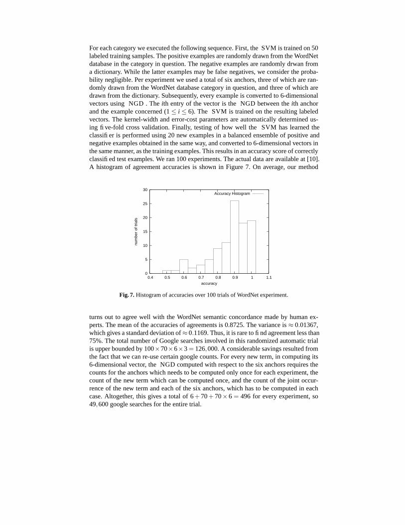
For each category we executed the following sequence. First, the SVM is trained on 50labeled training samples. The positive examples are randomly drawn from the WordNetdatabase in the category in question. The negative examples are randomly drwan froma dictionary. While the latter examples may be false negatives, we consider the proba-bility negligible. Per experiment we used a total of six anchors, three of which are ran-domly drawn from the WordNet database category in question, and three of which aredrawn from the dictionary. Subsequently, every example is converted to 6-dimensionalvectors using NGD . The ith entry of the vector is the NGD between the ith anchorand the example concerned (1 ≤ i ≤ 6). The SVM is trained on the resulting labeledvectors. The kernel-width and error-cost parameters are automatically determined us-ing five-fold cross validation. Finally, testing of how well the SVM has learned theclassifier is performed using 20 new examples in a balanced ensemble of positive andnegative examples obtained in the same way, and converted to 6-dimensional vectors inthe same manner, as the training examples. This results in an accuracy score of correctlyclassified test examples. We ran 100 experiments. The actual data are available at [10].A histogram of agreement accuracies is shown in Figure 7. On average, our method

0

5

10

15

20

25

30

0.4 0.5 0.6 0.7 0.8 0.9 1 1.1

num

ber

of tr

ials

accuracy

Accuracy Histogram

Fig. 7. Histogram of accuracies over 100 trials of WordNet experiment.

turns out to agree well with the WordNet semantic concordance made by human ex-perts. The mean of the accuracies of agreements is 0.8725. The variance is ≈ 0.01367,which gives a standard deviation of ≈ 0.1169. Thus, it is rare to find agreement less than75%. The total number of Google searches involved in this randomized automatic trialis upper bounded by 100×70×6×3 = 126,000. A considerable savings resulted fromthe fact that we can re-use certain google counts. For every new term, in computing its6-dimensional vector, the NGD computed with respect to the six anchors requires thecounts for the anchors which needs to be computed only once for each experiment, thecount of the new term which can be computed once, and the count of the joint occur-rence of the new term and each of the six anchors, which has to be computed in eachcase. Altogether, this gives a total of 6 + 70 + 70× 6 = 496 for every experiment, so49,600 google searches for the entire trial.

References

1. J.P. Bagrow, D. ben-Avraham, On the Google-fame of scientists and other populations, AIPConference Proceedings 779:1(2005), 81–89.

2. D. Benedetto, E. Caglioti, and V. Loreto, Language trees and zipping, Phys. Review Lett.,88:4(2002) 048702.

3. C.H. Bennett, P. Gacs, M. Li, P.M.B. Vitanyi, W. Zurek, Information Distance, IEEE Trans.Information Theory, 44:4(1998), 1407–1423. (Conference version: “Thermodynamics ofComputation and Information Distance,” In: Proc. 25th ACM Symp. Theory of Comput.,1993, 21-30.)

4. C.H. Bennett, M. Li, B. Ma, Chain letters and evolutionary histories, Scientific American,June 2003, 76–81.

5. C.J.C. Burges. A tutorial on support vector machines for pattern recognition, Data Miningand Knowledge Discovery, 2:2(1998),121–167.

6. X. Chen, B. Francia, M. Li, B. McKinnon, A. Seker, Shared information and program pla-giarism detection, IEEE Trans. Inform. Th., 50:7(2004), 1545–1551.

7. R. Cilibrasi, The CompLearn Toolkit, CWI, 2003–, http://www.complearn.org/8. P. Cimiano, S. Staab, Learning by Googling, SIGKDD Explorations, 6:2(2004), 24–33.9. W. Chai and B. Vercoe. Folk music classification using hidden Markov models. Proc. of

International Conference on Artificial Intelligence, 2001.10. R. Cilibrasi, P. Vitanyi, Automatic Meaning Discovery Using Google: 100 Experiments in

Learning WordNet Categories, 2004, http://www.cwi.nl/∼cilibrar/googlepaper/appendix.pdf11. R. Cilibrasi, R. de Wolf, P. Vitanyi. Algorithmic clustering of music based

on string compression, Computer Music J., 28:4(2004), 49-67. Web version:http://xxx.lanl.gov/abs/cs.SD/0303025

12. R. Cilibrasi, P.M.B. Vitanyi, Clustering by compression, IEEE Trans. Information Theory,51:4(2005), 1523- 1545. Web version: http://xxx.lanl.gov/abs/cs.CV/0312044

13. R. Cilibrasi, P. Vitanyi, Automatic meaning discovery using Google, Manuscript, CWI, 2004;http://arxiv.org/abs/cs.CL/0412098

14. R. Cilibrasi, P.M.B. Vitanyi, A New Quartet Tree Heuristic for Hierarchical Clustering, EU-PASCAL Statistics and Optimization of Clustering Workshop, 5-6 Juli 2005, London, UK.http://homepages.cwi.nl/ paulv/papers/quartet.pdf

15. R. Dannenberg, B. Thom, and D. Watson. A machine learning approach to musical stylerecognition, Proc. International Computer Music Conference, pp. 344-347, 1997.

16. R. Duda, P. Hart, D. Stork. Pattern Classification, John Wiley and Sons, 2001.17. The basics of Google search, http://www.google.com/help/basics.html.18. M. Grimaldi, A. Kokaram, and P. Cunningham. Classifying music by genre using the wavelet

packet transform and a round-robin ensemble. Technical report TCD-CS-2002-64, Trin-ity College Dublin, 2002. http://www.cs.tcd.ie/publications/tech-reports/reports.02/TCD-CS-2002-64.pdf

19. E. Keogh, S. Lonardi, and C.A. Rtanamahatana, Toward parameter-free data mining, In:Proc. 10th ACM SIGKDD Intn’l Conf. Knowledge Discovery and Data Mining, Seattle,Washington, USA, August 22—25, 2004, 206–215.

20. A.N. Kolmogorov. Three approaches to the quantitative definition of information, ProblemsInform. Transmission, 1:1(1965), 1–7.

21. A.N. Kolmogorov. Combinatorial foundations of information theory and the calculus ofprobabilities, Russian Math. Surveys, 38:4(1983), 29–40.

22. T. Landauer and S. Dumais, A solution to Plato’s problem: The latent semantic analysistheory of acquisition, induction and representation of knowledge, Psychol. Rev., 104(1997),211–240.

23. D. B. Lenat. Cyc: A large-scale investment in knowledge infrastructure, Comm. ACM,38:11(1995),33–38.

24. M.E. Lesk, Word-word associations in document retrieval systems, American Documenta-tion, 20:1(1969), 27–38.

25. M. Li and P.M.B. Vitanyi, Theory of thermodynamics of computation, Proc. IEEE Physics ofComputation Workshop, Dallas (Texas), Oct. 4-6, 1992, pp. 42-46. A full version (basicallythe here relevant part of [26]) appeared in the Preliminary Proceedings handed out at theWorkshop.

26. M. Li and P.M.B. Vitanyi, Reversibility and adiabatic computation: trading time and spacefor energy, Proc. Royal Society of London, Series A, 452(1996), 769-789.

27. M. Li and P.M.B. Vitanyi, An Introduction to Kolmogorov Complexity and its Applications,Springer-Verlag, New York, 2nd Edition, 1997.

28. X. Chen, S. Kwong, M. Li. A compression algorithm for DNA sequences based on ap-proximate matching. In: Proc. 10th Workshop on Genome Informatics (GIW), number 10in the Genome Informatics Series, Tokyo, December 14-15 1999. Also in Proc. 4th ACMRECOMB, 2000, p. 107.

29. M. Li, J.H. Badger, X. Chen, S. Kwong, P. Kearney, and H. Zhang, An information-basedsequence distance and its application to whole mitochondrial genome phylogeny, Bioinfor-matics, 17:2(2001), 149–154.

30. M. Li and P.M.B. Vitanyi, Algorithmic Complexity, pp. 376–382 in: International Encyclo-pedia of the Social & Behavioral Sciences, N.J. Smelser and P.B. Baltes, Eds., Pergamon,Oxford, 2001/2002.

31. M. Li, X. Chen, X. Li, B. Ma, P. Vitanyi. The similarity metric, IEEE Trans. Informa-tion Theory, 50:12(2004), 3250- 3264. (Conference version in: Proc. 14th ACM-SIAMSymposium on Discrete Algorithms, Baltimore, USA, 2003, pp 863-872.) Web version:http://xxx.lanl.gov/abs/cs.CC/0111054

32. M. Li, P. M. B. Vitanyi. An Introduction to Kolmogorov Complexity and Its Applications, 2ndEd., Springer-Verlag, New York, 1997.

33. S. L. Reed, D. B. Lenat. Mapping ontologies into cyc. Proc. AAAI Confer-ence 2002 Workshop on Ontologies for the Semantic Web, Edmonton, Canada.http://citeseer.nj.nec.com/509238.html

34. P. Scott. Music classification using neural networks, 2001.http://www.stanford.edu/class/ee373a/musicclassification.pdf

35. K. Strimmer, A. von Haeseler. Quartet puzzling: A quartet maximum likelihood method forreconstructing tree topologies, Mol Biol Evol, 1996, 13 pp. 964-969.

36. G.A. Miller et.al, WordNet, A Lexical Database for the English Language, Cognitive ScienceLab, Princeton University.http://www.cogsci.princeton.edu/∼wn

37. E. Terra and C. L. A. Clarke. Frequency Estimates for Statistical Word Similarity Measures.HLT/NAACL 2003, Edmonton, Alberta, May 2003. 37/162

38. P.-N. Tan, V. Kumar, J. Srivastava, Selecting the right interestingness measure for associatingpatterns. Proc. ACM-SIGKDD Conf. Knowledge Discovery and Data Mining, 2002, 491–502.

39. G. Tzanetakis and P. Cook, Music genre classification of audio signals, IEEE Transactionson Speech and Audio Processing, 10(5):293–302, 2002.

40. S. Wehner, Analyzing network traffic and worms using compression,http://arxiv.org/abs/cs.CR/0504045

41. Corpus collosal: How well does the world wide web rep-resent human language? The Economist, January 20, 2005.http://www.economist.com/science/displayStory.cfm?story id=3576374