DPRIETI Discussion Paper Series 10-E-057

Similarities and Differencesbetween the Manufacturing and the Service Sectors:

An empirical analysis of Japanese automobile related industries

KATO AtsuyukiRIETI

The Research Institute of Economy, Trade and Industryhttp://www.rieti.go.jp/en/

- 1 -

RIETI Discussion Paper Series 10-E-057

October 2010

Similarities and Differences between the Manufacturing and the Service Sectors: An Empirical Analysis of Japanese Automobile Related Industries†

Asian Development Bank Institute

And Research Institute of Economy, Trade and Industry, IAA

Atsuyuki KATO

Abstract

This paper examines the similarities and differences between the manufacturing and the

service sectors in terms of market power and productivity dispersion, using data of

Japanese automobile manufacturers and dealers. Applying a newly developed approach

proposed by Martin (2010), we estimate the firm-specific productivity and mark-up

under imperfect competition, and discuss features of them by industry. From those

estimates, we find that both industries have similar relations between productivity and

mark-up, and their transition probabilities are almost the same. On the other hand, the

roles of industries in the production process or the conditions of market competition are

different between those industries. In addition, the relations between business scale and

productivity are conflicting. As a whole, the implicit assumption that the service

industries are structurally different from manufacturing is controversial. However,

ignoring the differences in the conditions of their market competition possibly gives

significant bias to the policy implications.

Keywords: Productivity, Mark-up, Industrial Structure, Imperfect Competition

JEL Classification：D22, D43, L11

† The author would like to thank Sadao Nagaoka, Masahisa Fujita and other seminar participants at RIETI for their constructive comments. The author also wishes to thank Ralf Martin (London School of Economics) for allocating his STATA code to estimate firm-specific mark-up and productivity. This work was supported by KAKENHI (22653032). akato@adbi.org or kato-atsuyuki@rieti.go.jp

RIETI Discussion Papers Series aims at widely disseminating research results in the form of professional papers, thereby stimulating lively discussion. The views expressed in the papers are solely those of the author(s), and do not present those of the Research Institute of Economy, Trade and Industry.

- 2 -

1. Introduction

Recently, economists and policymakers have devoted a lot of attention to

productivity growth in the service sector. For almost four decades since the early 1960s,

service industries had been considered less productive or stagnant and this “productivity

paradox” was a key topic in empirical economics1. However, a revival of economic

growth in the U.S. driven by productivity growth in the service sector in the late 1990s

and the early 2000s made these views obsolete. It revealed that the service sector is not

always stagnant and that productivity growth plays a decisive role in achieving further

macroeconomic growth in advanced economies. Many papers have been dedicated to

understanding the factors causing this productivity growth, such as information and

communication technologies (ICTs), labour market flexibility, and deregulation. In

addition, the experiences that other advanced economies in Europe and Japan failed to

follow the U.S. sled light on the role of intangible assets2.

In those papers, many researchers and policymakers consider that manufacturing

and service production are different activities. However, that approach is really

controversial because the actual production is an intricate process of both manufacturing

and service activities. Manufacturing firms usually include service production in their

production process. Similarly, many forms of services are provided relying on

manufactured products. It indicates that the industry classification should be carefully

discussed to reflect these actual production processes at the aggregated levels. In

addition, it is meaningful to examine productivity of closely related industries between

both manufacturing and service sectors in empirical micro-econometric analysis.

1 Canadian Journal of Economics Vol. 32, No.9 (1999) 2 Corrado, Hulten and Sichel (2006a), Bloom and van Reenen (2007), and Miyagawa et al. (2010)

- 3 -

Without the activity level data in firms, it can be an alternative approach to examine

these complicated relationships.

In this paper, we discuss the latter issue using firm-level data of the Japanese

automobile related industries: automobile manufacturers including parts and accessories

(henceforth, Makers), and automobile dealers (henceforth, Dealers). As is well known,

the automobile manufacturing sector is a leading industry in Japan, and is thought to be

highly productive and innovative. In addition, Makers and Dealers are closely tied. For

example, Makers usually make their production plans following information about

customers’ preference, in order to assemble vehicles as semi-tailor made products. On

the other hand, Dealers propose various plans of purchasing to customers based on

production capacity of Makers3. Thus examining these industries allows us to further

investigate this issue. Applying a newly developed econometric approach by Martin

(2010) to these industries, we estimate the firm-specific mark-up and productivity, and

examine their dispersion and market structures.

The outline of this paper is as follows. In section 2, we briefly explain the model

and estimation method which we apply. Section 3 describes data used. In section 4, we

discuss the empirical results and their implications. And the conclusions are in the last

section.

2. Model

In this paper, we rely on an estimation method proposed by Martin (2010). To

avoid redundancy, we briefly show what the basic idea of this approach is, and what

we actually estimate, following his explanation. First, we assume that a firm follows a

3 This is relevant for new car sales. Dealers also have another market for used cars.

- 4 -

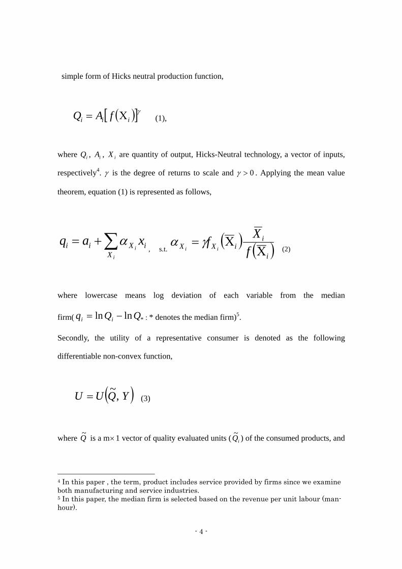
simple form of Hicks neutral production function,

iii fAQ (1),

where iQ , iA , iX are quantity of output, Hicks-Neutral technology, a vector of inputs,

respectively4. is the degree of returns to scale and 0 . Applying the mean value

theorem, equation (1) is represented as follows,

iX

Xii xaqi

i , s.t.

ii

iXX f

Xf

ii

(2)

where lowercase means log deviation of each variable from the median

firm( *lnln QQq ii : * denotes the median firm)5.

Secondly, the utility of a representative consumer is denoted as the following

differentiable non-convex function,

YQUU ,~

(3)

where Q~

is a m1 vector of quality evaluated units ( iQ~

) of the consumed products, and

4 In this paper , the term, product includes service provided by firms since we examine both manufacturing and service industries. 5 In this paper, the median firm is selected based on the revenue per unit labour (man-hour).

- 5 -

Y is income6. iQ~

= iiQ (the product of consumer’s valuation of the quality and the

quantity for firm i ’s product). Suppose each firm faces a downward sloping demand

curve conditional on the actions of other firms, then the demand function is written as

follows,

ii PDQ (4)7.

From equation (4), the price elasticity of demand for firm i ’s product is obtained as

i

ii P

PD

ln

ln

. Using it, the markup of firm i is defined as

i

i

1

1

1

.

Thirdly, firm i ’s profit ( i ) is written as follows,

iiiiii CQQP (5),

where iiC is the cost function of firm i . Since we assume all firms follow the profit

maximisation principle, the following first order condition is obtained,

iXiiiXi

iiiX

i

iii CQf

f

QQPf

f

QQP

(6).

Using XiXi WC ( XW is the marginal cost of X ) and i , equation (6) is rewritten

as follows,

6 m is the number of differentiated products. 7 Caplin and Nalebuff (1991)

- 6 -

XiiXi

ii Wf

f

QP

(7).

From equations (2) and (7), we obtain the following relation,

Xiiii

iXiX s

QP

XWi

(8),

where Xis represents the revenue share of variable X for firm i . Equation (8) indicates

that the firm-specific mark-up is obtained as a function of the revenue shares as follows,

iX

XiXii s

sS 1

(9).

On the other hand, firm i ’s revenue ( iii PQR ) is determined by production and

demand, and is represented as a function of them, iiii ARR ,, . Applying the

mean value theorem, it is also re-written as follows,

iA

iiiX

ii axr

(10),

where i

iXi X

R

ln

ln

and 2

XXiX

i

. i is an iid shock.

Among the input variables, capital ( k ) is usually assumed to be fixed at least in the

- 7 -

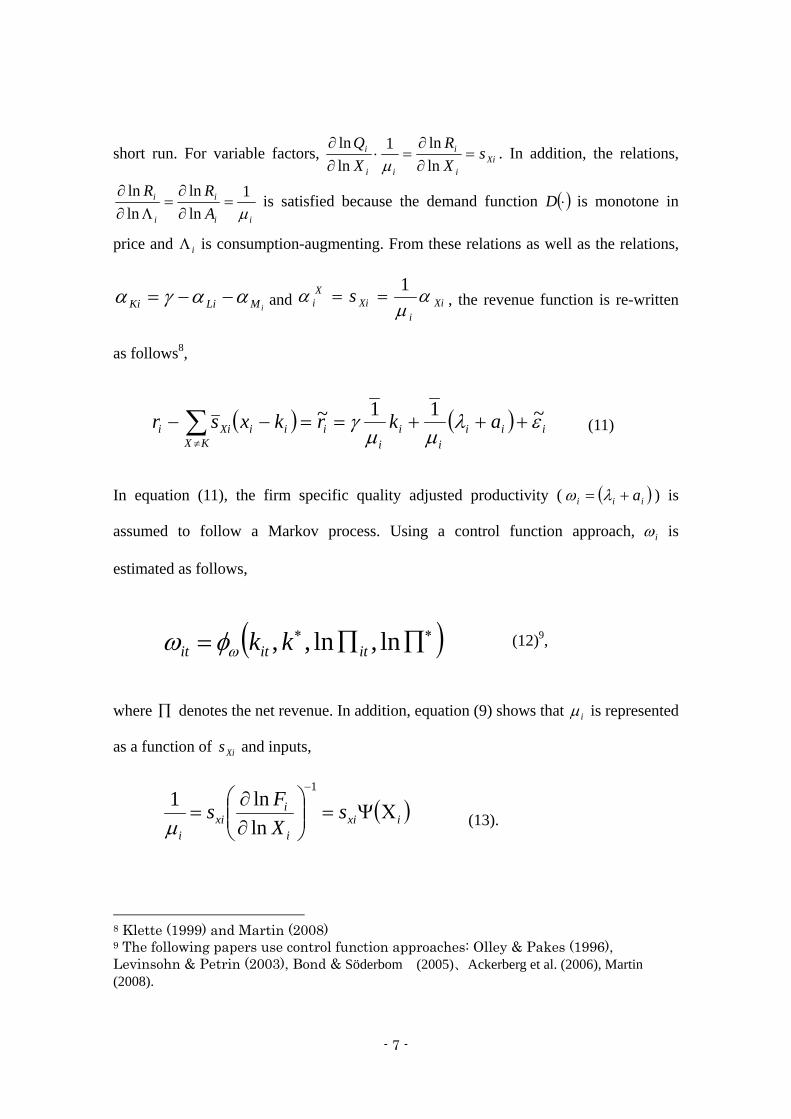
short run. For variable factors, Xii

i

ii

i sX

R

X

Q

ln

ln1

ln

ln

. In addition, the relations,

ii

i

i

i

A

RR

1

ln

ln

ln

ln

is satisfied because the demand function D is monotone in

price and i is consumption-augmenting. From these relations as well as the relations,

iMLiKi and Xii

XiX

i s

1 , the revenue function is re-written

as follows8,

(11)

In equation (11), the firm specific quality adjusted productivity ( iii a ) is

assumed to follow a Markov process. Using a control function approach, i is

estimated as follows,

(12)9,

where denotes the net revenue. In addition, equation (9) shows that i is represented

as a function of Xis and inputs,

(13).

8 Klette (1999) and Martin (2008) 9 The following papers use control function approaches: Olley & Pakes (1996), Levinsohn & Petrin (2003), Bond & Söderbom (2005)、Ackerberg et al. (2006), Martin (2008).

iiii

ii

iiiKX

Xii akrkxsr

~11~

ixii

ixi

i

sX

Fs

1

ln

ln1

ln,ln,, ititit kk

- 8 -

From this equation,

i 1

can also be written as a function of Xis and i . That is,

(14).

Finally equation (11) is estimated as follows,

(15)

where r is an unknown function and approximated by a polynomial. From equations

(11) and (14), over is obtained as follows,

(16)

where rit̂ is an estimate of r obtained in the second stage of equation (15).

The estimates of rescaled by are also used to recover it , using the following

equation,

itititit vP

ˆ,

ˆˆ 1

(17),

where itP̂ is the predicted exit probability which is estimated at the first stage of this

estimation procedure. Since the shock, it is independent of all predetermined variables

0000 lnln2

,,ln,ln xitxitxxitit ssssg

itxxitit

ritit kssg

00 ,,ln,ln

ˆˆ

titxtxittitrit ssr ln,ln,,,ln,ln~

- 9 -

including capital, we can use the following moment restrictions to estimate the

remaining parameters,

01 ititit vkXE (18).

3. Data

For this research, we construct the dataset based upon the Basic Survey of

Business Structure and Activity (BSBSA) for the period between 1995 and 200510. This

is a complete enumeration for firms whose workers are more than 50 or capital is over

30 million Japanese yen in manufacturing and various service industries. From this

statistics, we use total sales as data of total revenues of firms. The proxy of accumulated

capital is the tangible fixed assets. Labour input is calculated as man-hours11. Following

Morikawa (2010), we separately calculate regular and contingent workers and add them

up. In addition, the total wage is used as the labour cost. As a proxy for intermediate

inputs, the amount of purchase is sometimes used. However, we do not follow it

because that data includes many zeros and blanks. Instead we construct that variable

from financial data following Tokui, Inui and Kim (2007) and Kim, Kwon and Fukao

(2007),

DTDepTWSGACOGSInputteIntermedia & ,

where COGS, SGA, TW, Dep and T&D are the cost of goods sold, the selling and

10 This statistics is annually compiled by the Ministry of Economy, Trade and Industry (METI) Japan. 11 The data of working hours are available from Monthly Labour Survey.

- 10 -

general administrative expenses, the total wages, the depreciation and the tax and dues,

respectively. In constructing our dataset, we rule out the firms that report zero or

negative values as the number of regular workers, the tangible fixed assets, total wage,

or intermediate inputs. In many existing papers, capital stock data are constructed by

subtracting the land from the tangible fixed assets. However we do not follow them

because we consider the location of (or access to) business possibly has a crucial role in

production, and the land value can capture such information.

4. Empirical Results

In this section, we discuss empirical results and their implications. We focus on the

following issues: 1) Are there some differences in the distributions of productivity and

mark-up levels between Dealers and Makers, 2) What relations can we find between

productivity and market power, 3) Are there some differences in the transition dynamics

between them, and 4) Is business scale or employment structure related to productivity

and pricing power?12. From these analyse, we discuss similarities and differences of

Dealers and Makers, and obtain reliable implication.

The first issue is related to the question of whether productivity of manufacturing

firms is higher than that of service firms as generally believed. Although this view

widely prevails, it is somewhat controversial because of conceptual and methodological

problems. In order to examine this issue, we estimate productivity and mark-up using a

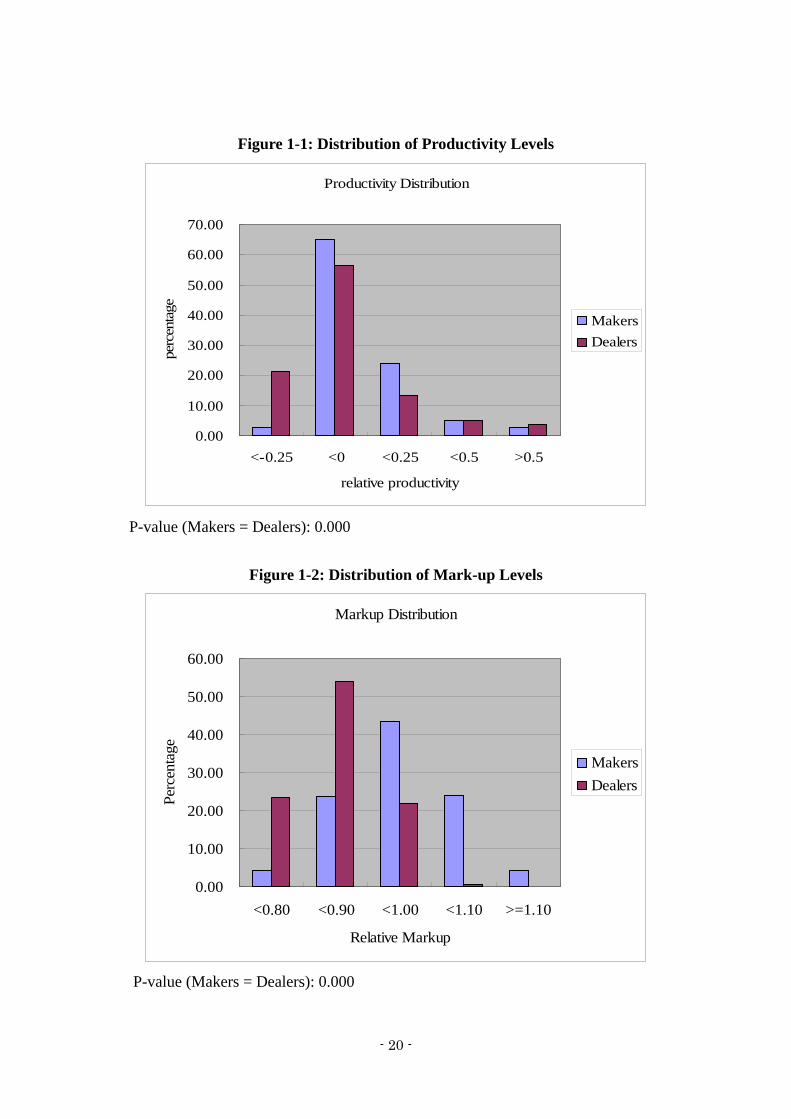
combined data of Dealers and Makers. Figures 1-1 and 1-2 show the distributions of

them. They indicate that productivity distributions are similar between Dealers and

12 The foreign capital ratio is not examined because most of the firms in Dealers do not accept foreign capital at all and comparison between domestic and foreign firms is somewhat controversial.

- 11 -

Makers while mark-up distributions are very different. Obviously, Makers obtain higher

pricing powers than Dealers13. It might reveal that Dealers and Makers have different

roles in sets of production processes if both firms are highly correlated. In this case, the

above largely accepted view is meaningless because the lower TFP of the service sector

in conventional approaches such as an index number approach only means that it does

not have roles to obtain higher pricing power in the whole production process.

On the other hand, it possibly reflects the differences of the conditions on

competition between Dealers and Makers. If it is even more difficult for Dealers to

differentiate their products than Makers, the mark-up levels of Dealers tend to be lower

than those of Makers. This view seems to be reasonable to some extent because Makers

likely specialise certain technologies or products while Dealers usually compete each

other in more generalised markets including used car markets. Even in this case, the

general view is less supported as well because productivity of Dealers is not

significantly lower than that of Makers. These discussions reveal that productivity

analysis might give an irrelevant implication if the mark-up is ignored.

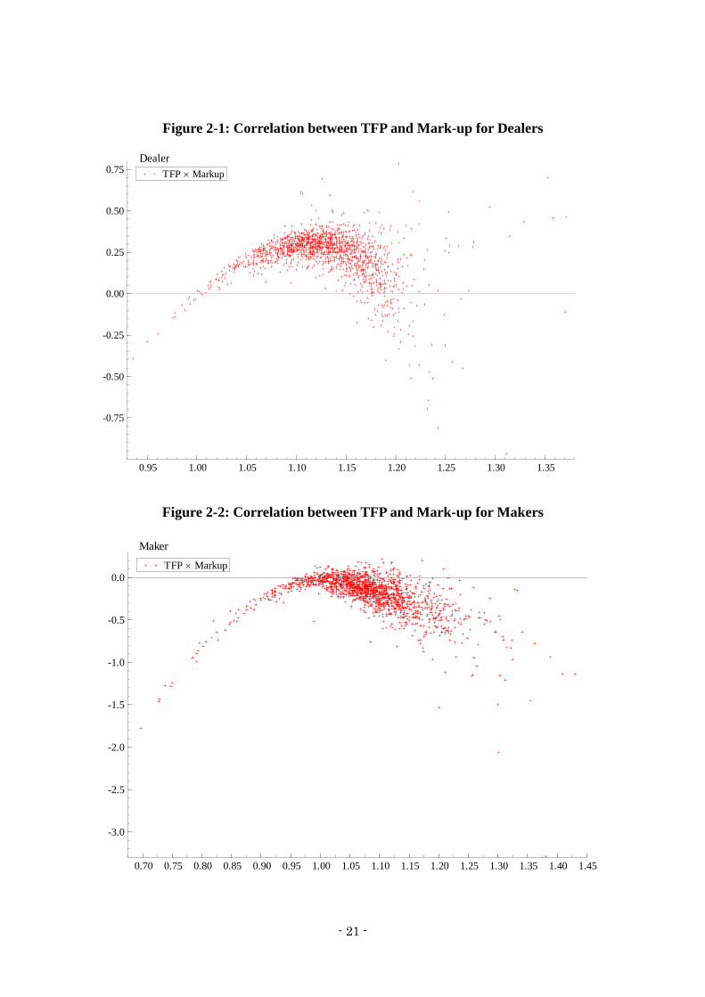
For the second issues, we estimate both performances industry by industry. Figures

2-1 and 2-2 show the results. They reveal that the correlations between mark-up and

productivity are similar between Dealers and Makers. It means that these industries

have the similar properties on the profit maximisation activities. As a whole, the

productivity levels of firms with respect to their mark-ups are scattered as inverse U-

shape distributions in both industries. In addition, the dispersion of productivity levels is

larger for the firms with higher mark-ups than those with lower ones.

These results imply that increasing in the firm specific mark-up does not always

13 The differences of the price levels between industries are not crucial because they are relatively stable during the examined period.

- 12 -

result in improving the productivity level. Rather, firms seem to have various strategies

to pursue their profit maximisation. Some firms focus on improving their productivity at

the expense of their pricing power. These firms are thought to provide more

standardised or substitutable products. Others put much weight in obtaining larger

pricing powers through differentiation. Those firms possibly use less efficient

technologies for mass production14. In both manufacturing and service industries, both

groups of firms coexist. On the other hand, firms with relatively smaller market powers

are also less productive in both industries. It implies that there is a threshold point of the

mark-up levels to join the pricing power or productivity competition for each industry.

In addition, the finding that the mark-up distribution for Makers is larger than that for

Dealers is thought to support the hypothesis in the previous paragraph that Makers are

more likely differentiated than Dealers.

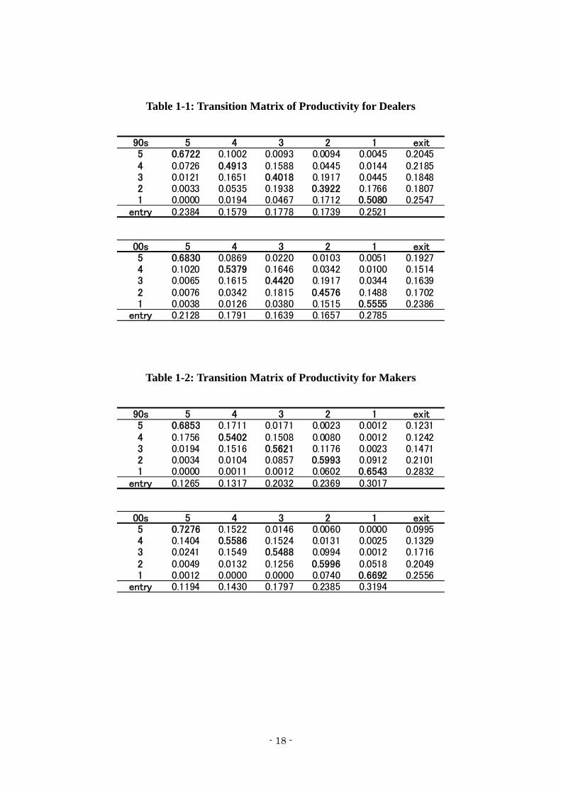
The third issue is examined by transition matrices. Tables 1-1 and 1-2 obviously

show that the transitions of firms are similar between both industries with respect to

productivity. In both industries, neither a leapfrogging nor a free fall is detected. It

means that relative levels of firm-specific productivities are persistent. In particular, the

probabilities on the top and bottom edges of the diagonal are higher than those on the

middle. These tables also imply that such persistency is not affected by a business cycle

because the transition probabilities are not significantly changed between the later half

of the 1990s (recession) and the early half of the 2000s (boom). These results cast doubt

on views that manufacturing industries are Schumpeterian-innovative while service

industries are more stagnant.

As well as productivity, relative levels of firm-specific mark-ups are also persistent.

14 For example, firms providing luxury brand items seem to follow this strategy.

- 13 -

Tables 2-1 and 2-2 show the transition probabilities of them. In particular, firms in the

bottom group of Makers are more likely to stay the same group. It means that it is quite

difficult for firms to slip out of the position where their price making power is lowest

once they fall in. In addition, this finding implies that it is difficult for those firms to

take the productivity strategy since they are also less productive as we discussed.

Interestingly, the percentage that firms continue to stay in the bottom range is higher in

Makers than Dealers. It indicates that the fetters of poor pricing powers are tighter in the

former than the latter.

As the fourth issue, we examines if the larger firms are more productive than the

smaller ones and if increase in contingent workers has a positive correlation with

productivity. For the first question, there is a complicated view. It is not always thought

that the productivity of the small firms is lower than that of the large firms in the

manufacturing sector while the small firms which account for the lion’s share in the

retail trade industry are considered to make that industry less productive15. On the other

hand, the second question is highly related to the issue of the structural change of the

employment. To discuss them, we separate firms in each industry into three groups with

respect to their business scale and their shares of contingent workers.

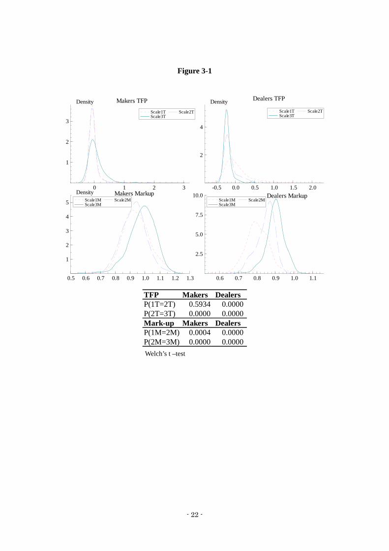
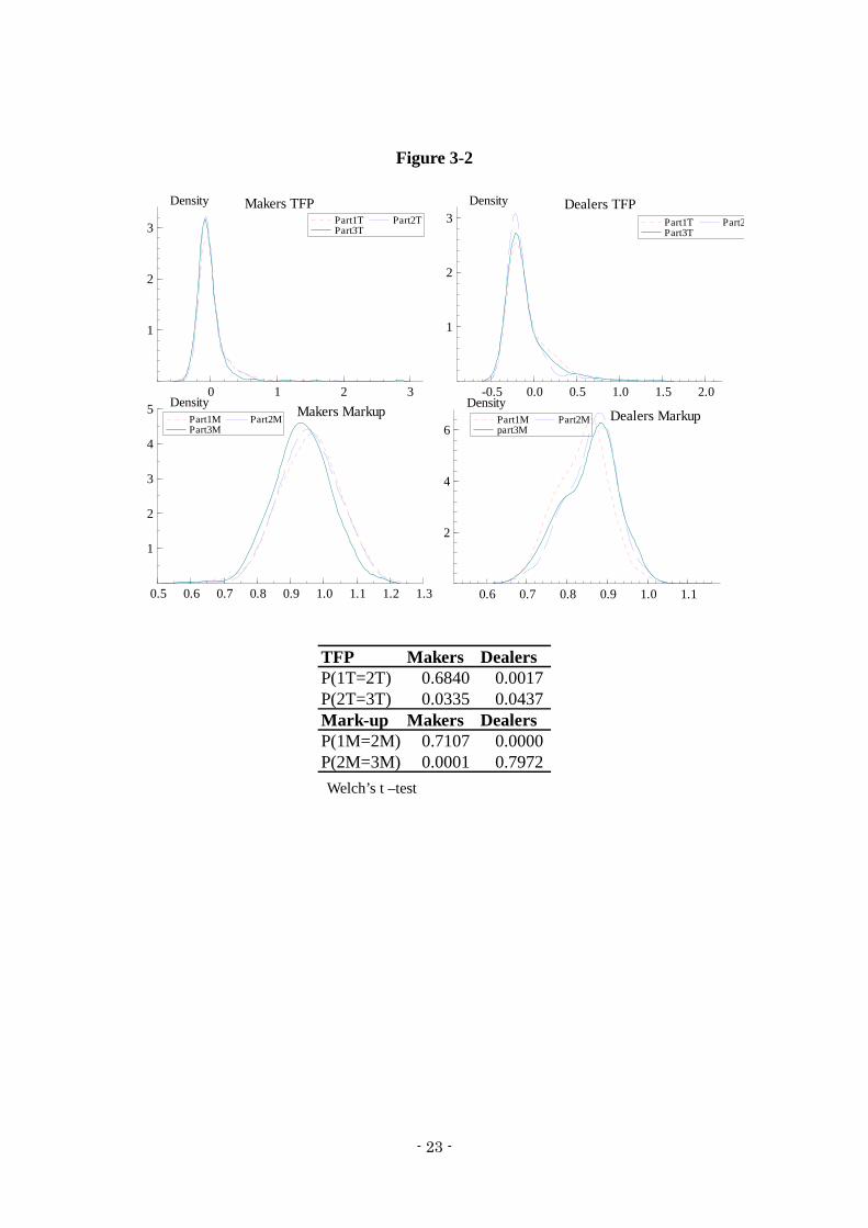
Figures 3-1 and 3-2 show the kernel density of those groups. In these figures, 1, 2 and

3 are corresponding to small, medium and large, respectively. T and M also represent

TFP and Mark-up, respectively. These figures give complicated views. For business

scale, the productivity of the large firms is higher than those of others in Makers while

Small > Medium > Large in Dealers. On the other hand, the large firms have the higher

mark-up levels than those of others in both industries. Although the interpretation of

15 McKinsey Global Institute (2000)

- 14 -

these results is limited because our data do not include the firms whose workers are less

than 50 or whose capital are less than 30 million Japanese yen, they imply that the view

that the small firms are less productive is not always confirmed for the retail trade

industry. The results indicate that the large firms have advantages for pricing powers

rather than productivity.

For the second question, Figure 3-2 reveals that increase in the contingent workers is

not positively correlated with productivity or market power in both industries. Instead,

for Makers, the larger share of the contingent workers seems to be negatively correlated

with the performances. This finding gives an important implication. Although firms

have expanded the share of the contingent workers to reduce costs, those efforts do not

yield better performances in more differentiated markets. For Dealers, it is difficult to

find a consistent relation between them. It implies that those efforts do not always result

in higher performances even in more generalised markets. These findings should be

noted for further discussion about the reform of the labour market

5. Concluding Remarks

In this paper, we estimate the firm-specific mark-up and productivity under imperfect

competition for automobile manufacturers and dealers, and discuss the similarities and

differences between them using those estimates. Our findings reveal the basic properties

on their profit maximisation activities and the transition dynamics are very similar each

other. Some firms pursue the profit maximisation through productivity improvement for

mass production while others do it through increasing their pricing powers. Since their

profit maximisation activities are significantly diversified, we should carefully consider

for what groups of firms a certain policy supports in devising industrial policies. In

- 15 -

addition, the relative positions of firms with respect to both productivity and mark-up

are very persistent. It indicates that the view that the manufacturing sector is more

Schumpeterian-innovative than the service sector is very controversial. It also gives a

bias to the policy implication of the productivity analysis if ignored.

On the other hand, our estimates also show that the distributions of the firm-specific

pricing powers are very different between Makers and Dealers although those of the

productivity are not much different. It might reflect the difference of their roles in the

whole production process or the differences in the conditions of their market

competition. In addition, the correlations between business scale and productivity are

heterogeneous between them as well. The relations between the employment structure

and the firm performances are not consistent between them, either.

These findings imply that the simple separation between the manufacturing and the

service sectors in the productivity analysis are not much meaningful. Instead, it is

important to examine it by carefully considering the roles of the industry in the whole

production process and the structures of their markets.

Although this paper provides some additional contributions for productivity analysis,

there are still some remained problems. First, the assumption of the identical degree of

returns to scale is somewhat controversial. For further discussion of productivity

analysis, we should examine the possibility that is varies between and within industries.

Secondly, we do not directly examine the causal relations between the performances and

properties of firms by a regression analysis because of some methodological problems.

But, it is better to devise an econometric analysis to obtain more robust implications.

Furthermore, we should integrate our analysis into the input-output analysis and obtain

a comprehensive view. All of them are the future research topics.

- 16 -

References

Ackerberg D., K. Caves and G. Frazer (2006), “Structural Identification of Production

Functions”, Working Paper, (available on the first author’s website).

Bond S. and M. Söderbom (2005), “Adjustment Costs and the Identification of Cobb

Douglas Production Function”, IFS Working Paper, W05/04.

Bloom N. and J. van Reenen (2007), “Measuring and Explaining Management Practices

Across Firms and Countries”, Quarterly Journal of Economics, 122 (4), 1351-1408.

Caplin A. and B. Nalebuff (1991), “Aggregation and Imperfect Competition: On the

Existence of Equilibrium”, Econometrica, 59 (1), 25-59.

Corrado C., C. R. Hulten and D. E. Sichel (2006), “Intangible Capital and Economic

Growth”, NBER Working Paper, 11948.

Diewert W. E. (1999), “Special Issue on Service Sector Productivity Paradox,”

Canadian Journal of Economics, 32 (2).

Kim Y. G., H. U. Kwon and K. Fukao (2007), “Entry and Exit of Companies and

Establishments, and Productivity at the Industry Level (in Japanese)”, RIETI

Discussion Paper, 07-J-022.

Klette T. J. (1999), “Market Power, Scale Economies, and Productivity: Estimates from

a Panel of Establishment Data”, Journal of Industrial Economics, XLVII (4), 451-

476.

Levinsohn J. and A. Petrin (2003), “Estimating Production Functions Using Inputs to

- 17 -

Control for Unobservables”, Review of Economic Studies, 70 (2), 317-342.

Martin R. (2010), “Productivity Spreads, Market Power Spreads, and Trade”, mimeo.

McKinsey Global Institute, 2000, “Why the Japanese Economy Is Not Growing: Micro

Barriers to Productivity Growth”, McKinsey Global Institute.

Miyagawa T., K. Lee, S. Kabe, J. Lee, H. Kim, Y. Kim and K. Edamura (2009),

“Management Practices and Firm Performance in Japanese and Korean Firms: An

Empirical Analysis using Interview Surveys”, RIETI Discussion Paper, 10-E-013.

Morikawa M. (2010), “Working Hours of Part-timers and the Measurement of Firm-

Level Productivity (in Japanese)”, RIETI Discussion Paper, 10-J-22.

Olley S., and A. Pakes (1996), “The Dynamics of Productivity in the

Telecommunication Equipment Industry”, Econometrica, 64, 1263-1297.

Tokui J., T. Inui and Y. G. Kim (2007), “The Embodied Technical Progress and the

Average Vintage of Capital (in Japanese)”, RIETI Discussion Paper, 07-J-035.

- 18 -

Table 1-1: Transition Matrix of Productivity for Dealers

90s 5 4 3 2 1 exit5 0.6722 0.1002 0.0093 0.0094 0.0045 0.20454 0.0726 0.4913 0.1588 0.0445 0.0144 0.21853 0.0121 0.1651 0.4018 0.1917 0.0445 0.18482 0.0033 0.0535 0.1938 0.3922 0.1766 0.18071 0.0000 0.0194 0.0467 0.1712 0.5080 0.2547

entry 0.2384 0.1579 0.1778 0.1739 0.2521

00s 5 4 3 2 1 exit5 0.6830 0.0869 0.0220 0.0103 0.0051 0.19274 0.1020 0.5379 0.1646 0.0342 0.0100 0.15143 0.0065 0.1615 0.4420 0.1917 0.0344 0.16392 0.0076 0.0342 0.1815 0.4576 0.1488 0.17021 0.0038 0.0126 0.0380 0.1515 0.5555 0.2386

entry 0.2128 0.1791 0.1639 0.1657 0.2785

Table 1-2: Transition Matrix of Productivity for Makers

90s 5 4 3 2 1 exit5 0.6853 0.1711 0.0171 0.0023 0.0012 0.12314 0.1756 0.5402 0.1508 0.0080 0.0012 0.12423 0.0194 0.1516 0.5621 0.1176 0.0023 0.14712 0.0034 0.0104 0.0857 0.5993 0.0912 0.21011 0.0000 0.0011 0.0012 0.0602 0.6543 0.2832

entry 0.1265 0.1317 0.2032 0.2369 0.3017

00s 5 4 3 2 1 exit5 0.7276 0.1522 0.0146 0.0060 0.0000 0.09954 0.1404 0.5586 0.1524 0.0131 0.0025 0.13293 0.0241 0.1549 0.5488 0.0994 0.0012 0.17162 0.0049 0.0132 0.1256 0.5996 0.0518 0.20491 0.0012 0.0000 0.0000 0.0740 0.6692 0.2556

entry 0.1194 0.1430 0.1797 0.2385 0.3194

- 19 -

Table 2-1: Transition Matrix of Mark-up for Dealers

90s 5 4 3 2 1 exit5 0.6277 0.1657 0.0249 0.0067 0.0011 0.17394 0.1706 0.4551 0.1603 0.0296 0.0000 0.18443 0.0246 0.1655 0.4514 0.1519 0.0056 0.20092 0.0059 0.0183 0.1638 0.5056 0.0900 0.21641 0.0024 0.0000 0.0033 0.0972 0.6295 0.2676

entry 0.1604 0.1865 0.1841 0.1942 0.2747

00s 5 4 3 2 1 exit5 0.6294 0.1745 0.0305 0.0037 0.0000 0.16194 0.1509 0.4808 0.1933 0.0178 0.0000 0.15733 0.0243 0.1796 0.4664 0.1486 0.0077 0.17472 0.0050 0.0308 0.1339 0.5234 0.1168 0.18881 0.0000 0.0012 0.0051 0.1214 0.6380 0.2342

entry 0.2071 0.1414 0.1871 0.2017 0.2626

Table 2-2: Transition Matrix of Mark-up for Makers

90s 5 4 3 2 1 exit5 0.5890 0.1093 0.0194 0.0046 0.0000 0.27764 0.1347 0.5138 0.1447 0.0160 0.0011 0.18973 0.0170 0.1847 0.4768 0.1154 0.0046 0.20152 0.0012 0.0149 0.1624 0.6141 0.0754 0.13211 0.0011 0.0023 0.0057 0.0990 0.8043 0.0876

entry 0.3020 0.1991 0.2218 0.1696 0.1229

00s 5 4 3 2 1 exit5 0.5824 0.1453 0.0145 0.0061 0.0000 0.25164 0.1152 0.5029 0.1689 0.0290 0.0025 0.18153 0.0096 0.1413 0.5078 0.1665 0.0095 0.16532 0.0048 0.0180 0.1525 0.5783 0.0955 0.14981 0.0000 0.0012 0.0097 0.0747 0.7987 0.1169

entry 0.3285 0.2245 0.1683 0.1668 0.1107

- 20 -

Figure 1-1: Distribution of Productivity Levels

Productivity Distribution

0.00

10.00

20.00

30.00

40.00

50.00

60.00

70.00

<-0.25 <0 <0.25 <0.5 >0.5

relative productivity

perc

enta

ge

Makers

Dealers

P-value (Makers = Dealers): 0.000

Figure 1-2: Distribution of Mark-up Levels

Markup Distribution

0.00

10.00

20.00

30.00

40.00

50.00

60.00

<0.80 <0.90 <1.00 <1.10 >=1.10

Relative Markup

Per

cent

age

Makers

Dealers

P-value (Makers = Dealers): 0.000

- 21 -

Figure 2-1: Correlation between TFP and Mark-up for Dealers

0.95 1.00 1.05 1.10 1.15 1.20 1.25 1.30 1.35

-0.75

-0.50

-0.25

0.00

0.25

0.50

0.75Dealer

TFP Markup

Figure 2-2: Correlation between TFP and Mark-up for Makers

0.70 0.75 0.80 0.85 0.90 0.95 1.00 1.05 1.10 1.15 1.20 1.25 1.30 1.35 1.40 1.45

-3.0

-2.5

-2.0

-1.5

-1.0

-0.5

0.0

Maker

TFP Markup

- 22 -

Figure 3-1

0 1 2 3

1

2

3

Density Makers TFP

Scale1T Scale3T

Scale2T

-0.5 0.0 0.5 1.0 1.5 2.0

2

4

Density Dealers TFP

Scale1T Scale3T

Scale2T

0.5 0.6 0.7 0.8 0.9 1.0 1.1 1.2 1.3

1

2

3

4

5

Density Makers MarkupScale1M Scale3M

Scale2M

0.6 0.7 0.8 0.9 1.0 1.1

2.5

5.0

7.5

10.0 Dealers MarkupScale1M Scale3M

Scale2M

TFP Makers DealersP(1T=2T) 0.5934 0.0000P(2T=3T) 0.0000 0.0000Mark-up Makers DealersP(1M=2M) 0.0004 0.0000P(2M=3M) 0.0000 0.0000

Welch’s t –test

- 23 -

Figure 3-2

0 1 2 3

1

2

3

Density Makers TFPPart1T Part3T

Part2T

-0.5 0.0 0.5 1.0 1.5 2.0

1

2

3Density Dealers TFP

Part1T Part3T

Part2

0.5 0.6 0.7 0.8 0.9 1.0 1.1 1.2 1.3

1

2

3

4

5 DensityMakers Markup

Part1M Part3M

Part2M

0.6 0.7 0.8 0.9 1.0 1.1

2

4

6

DensityDealers MarkupPart1M

part3M Part2M

TFP Makers DealersP(1T=2T) 0.6840 0.0017P(2T=3T) 0.0335 0.0437Mark-up Makers DealersP(1M=2M) 0.7107 0.0000P(2M=3M) 0.0001 0.7972

Welch’s t –test