simhydraulics user's guide - dphu · directions; directional valves bypassed by a huge...

SimHydraulics®

User's Guide

R2015a

How to Contact MathWorks

Latest news: www.mathworks.com

Sales and services: www.mathworks.com/sales_and_services

User community: www.mathworks.com/matlabcentral

Technical support: www.mathworks.com/support/contact_us

Phone: 508-647-7000

The MathWorks, Inc.3 Apple Hill DriveNatick, MA 01760-2098

SimHydraulics® User's Guide© COPYRIGHT 2006–2015 by The MathWorks, Inc.The software described in this document is furnished under a license agreement. The software may be usedor copied only under the terms of the license agreement. No part of this manual may be photocopied orreproduced in any form without prior written consent from The MathWorks, Inc.FEDERAL ACQUISITION: This provision applies to all acquisitions of the Program and Documentationby, for, or through the federal government of the United States. By accepting delivery of the Programor Documentation, the government hereby agrees that this software or documentation qualifies ascommercial computer software or commercial computer software documentation as such terms are usedor defined in FAR 12.212, DFARS Part 227.72, and DFARS 252.227-7014. Accordingly, the terms andconditions of this Agreement and only those rights specified in this Agreement, shall pertain to andgovern the use, modification, reproduction, release, performance, display, and disclosure of the Programand Documentation by the federal government (or other entity acquiring for or through the federalgovernment) and shall supersede any conflicting contractual terms or conditions. If this License failsto meet the government's needs or is inconsistent in any respect with federal procurement law, thegovernment agrees to return the Program and Documentation, unused, to The MathWorks, Inc.

Trademarks

MATLAB and Simulink are registered trademarks of The MathWorks, Inc. Seewww.mathworks.com/trademarks for a list of additional trademarks. Other product or brandnames may be trademarks or registered trademarks of their respective holders.Patents

MathWorks products are protected by one or more U.S. patents. Please seewww.mathworks.com/patents for more information.

www.mathworks.com

www.mathworks.com/sales_and_services

www.mathworks.com/matlabcentral

www.mathworks.com/support/contact_us

http://www.mathworks.com/trademarks

http://www.mathworks.com/patents

Revision History

March 2006 Online only New for Version 1.0 (Release 2006a+)September 2006 Online only Revised for Version 1.1 (Release 2006b)March 2007 Online only Revised for Version 1.2 (Release 2007a)September 2007 Online only Revised for Version 1.2.1 (Release 2007b)March 2008 Online only Revised for Version 1.3 (Release 2008a)October 2008 Online only Revised for Version 1.4 (Release 2008b)March 2009 Online only Revised for Version 1.5 (Release 2009a)September 2009 Online only Revised for Version 1.6 (Release 2009b)March 2010 Online only Revised for Version 1.7 (Release 2010a)September 2010 Online only Revised for Version 1.8 (Release 2010b)April 2011 Online only Revised for Version 1.9 (Release 2011a)September 2011 Online only Revised for Version 1.10 (Release 2011b)March 2012 Online only Revised for Version 1.10.1 (Release 2012a)September 2012 Online only Revised for Version 1.11 (Release 2012b)March 2013 Online only Revised for Version 1.12 (Release 2013a)September 2013 Online only Revised for Version 1.13 (Release 2013b)March 2014 Online only Revised for Version 1.14 (Release 2014a)October 2014 Online only Revised for Version 1.15 (Release 2014b)March 2015 Online only Revised for Version 1.16 (Release 2015a)

v

Contents

Getting Started1

SimHydraulics Product Description . . . . . . . . . . . . . . . . . . . . 1-2Key Features . . . . . . . . . . . . . . . . . . . . . . . . . . . . . . . . . . . . . 1-2

SimHydraulics Assumptions and Limitations . . . . . . . . . . . . 1-3

Simulating Hydraulic Models . . . . . . . . . . . . . . . . . . . . . . . . . 1-4Simulation Basics . . . . . . . . . . . . . . . . . . . . . . . . . . . . . . . . . 1-4Selecting a Solver . . . . . . . . . . . . . . . . . . . . . . . . . . . . . . . . . 1-4Specifying Simulation Accuracy/Speed Tradeoff . . . . . . . . . . 1-5Nonphysical Values During Simulation . . . . . . . . . . . . . . . . . 1-5Troubleshooting Hydraulic Models . . . . . . . . . . . . . . . . . . . . 1-6

Model Sharing . . . . . . . . . . . . . . . . . . . . . . . . . . . . . . . . . . . . . . 1-8

Modeling Hydraulic Systems2

SimHydraulics Block Libraries . . . . . . . . . . . . . . . . . . . . . . . . 2-2Library Structure Overview . . . . . . . . . . . . . . . . . . . . . . . . . 2-2Using the Simulink Library Browser to Access the Block

Libraries . . . . . . . . . . . . . . . . . . . . . . . . . . . . . . . . . . . . . . 2-2Using the Command Prompt to Access the Block Libraries . . 2-3

Modeling Hydraulic Power and Control Systems . . . . . . . . . 2-5

Essential Hydraulic Modeling Techniques . . . . . . . . . . . . . . . 2-6Overview of Modeling Rules . . . . . . . . . . . . . . . . . . . . . . . . . 2-6Working with Fluids . . . . . . . . . . . . . . . . . . . . . . . . . . . . . . . 2-7

vi Contents

Creating and Simulating a Simple Hydraulic Model . . . . . . . 2-9Building a SimHydraulics Diagram . . . . . . . . . . . . . . . . . . . . 2-9Modifying Initial Settings . . . . . . . . . . . . . . . . . . . . . . . . . . 2-16Running the Simulation . . . . . . . . . . . . . . . . . . . . . . . . . . . 2-20Adjusting the Parameters . . . . . . . . . . . . . . . . . . . . . . . . . . 2-22

Modeling Power Units . . . . . . . . . . . . . . . . . . . . . . . . . . . . . . . 2-27

Modeling Directional Valves . . . . . . . . . . . . . . . . . . . . . . . . . 2-31Types of Directional Valves . . . . . . . . . . . . . . . . . . . . . . . . . 2-314-Way Directional Valve Configurations . . . . . . . . . . . . . . . 2-32Building Blocks and How to Use Them . . . . . . . . . . . . . . . . 2-36Build a Custom Directional Valve . . . . . . . . . . . . . . . . . . . . 2-40

Modeling Low-Pressure Fluid Transportation Systems . . . 2-44How Fluid Transportation Systems Differ from Power and

Control Systems . . . . . . . . . . . . . . . . . . . . . . . . . . . . . . . 2-44Available Blocks and How to Use Them . . . . . . . . . . . . . . . 2-46Low-Pressure Fluid Transportation System . . . . . . . . . . . . 2-48

1

Getting Started

• “SimHydraulics Product Description” on page 1-2• “SimHydraulics Assumptions and Limitations” on page 1-3• “Simulating Hydraulic Models” on page 1-4• “Model Sharing” on page 1-8

1 Getting Started

1-2

SimHydraulics Product DescriptionModel and simulate hydraulic systems

SimHydraulics provides component libraries for modeling and simulating hydraulicsystems. It includes models of hydraulic components, such as pumps, valves, actuators,pipelines, and hydraulic resistances. You can use these components to model fluid powersystems such as front-loader, power steering, and landing gear actuation systems. Fuelsupply and water supply systems can also be modeled using SimHydraulics.

SimHydraulics models can be used to develop control systems and test system-levelperformance. You can parameterize your models using MATLAB® variables andexpressions, and design control systems for your hydraulic system in Simulink®. Youcan add electrical, mechanical, pneumatic, and other components to your hydraulicmodel using Simscape™ and test them in a single simulation environment. To deploymodels to other simulation environments, including hardware-in-the-loop (HIL) systems,SimHydraulics supports C-code generation.

Key Features

• Pump models, including centrifugal, jet, and axial-piston pumps• Directional valve models, including check valves and common configurations for 2-, 4-,

and 6-way valves• Flow and pressure control valve models, including ball, poppet, and pressure relief

valves• Translational and rotational actuator models, including optional friction and

centrifugal forces• Tank and pipe models with elevation effects for modeling fluid transportation systems• Customizable library of common hydraulic fluids• Ability to extend component libraries using the Simscape language• Support for C-code generation

SimHydraulics Assumptions and Limitations

1-3

SimHydraulics Assumptions and Limitations

SimHydraulics software performs transient analysis of hydro-mechanical systems.You may be able to use the higher-level library blocks, or you may need to build youractuators out of the lower-level library blocks. SimHydraulics software is specificallydeveloped to cover modeling scenarios with hydraulic actuators as part of a controlsystem. It is also appropriate for systems that allow consideration in lumped parameters.

SimHydraulics software is based on the assumption that fluid temperature remainsconstant during the simulated time interval, and this temperature must be set as aparameter together with the relative amount of entrapped air.

1 Getting Started

1-4

Simulating Hydraulic Models

In this section...

“Simulation Basics” on page 1-4“Selecting a Solver” on page 1-4“Specifying Simulation Accuracy/Speed Tradeoff” on page 1-5“Nonphysical Values During Simulation” on page 1-5“Troubleshooting Hydraulic Models” on page 1-6

Simulation Basics

SimHydraulics software gives you multiple ways to simulate and analyze hydraulicpower and control systems in the Simulink environment. Running a hydraulic simulationis similar to running a simulation of any other Simscape model. See “Simulation” in theSimscape documentation for a discussion of the following topics:

• Explanation of how SimHydraulics software validates and simulates a model• Specifics of using Simulink linearization commands in SimHydraulics models• Generating code for SimHydraulics models• Restrictions and limitations on using Simulink tools in SimHydraulics models

All these aspects of simulating SimHydraulics models are exactly the same as forSimscape models.

Selecting a Solver

SimHydraulics software supports all of the continuous-time solvers that Simscapesupports. For more information, see “Setting Up Solvers for Physical Models” in theSimscape documentation.

You can select any of the supported solvers for running a SimHydraulics simulation.The variable-step solvers, ode23t and ode15s, are recommended for most applicationsbecause they run faster and work better for systems with a range of both fast and slowdynamics.

To use Simulink Coder™ software to generate standalone C or C++ code from yourmodel, you must use the ode14x solver. For more information about code generation, see“Code Generation” in the Simscape documentation.


1-5

Specifying Simulation Accuracy/Speed Tradeoff

To trade off accuracy and simulation time, adjust one or more of the followingparameters:

• Relative tolerance (in the Configuration Parameters dialog box)• Absolute tolerance (in the Configuration Parameters dialog box)• Max step size (in the Configuration Parameters dialog box)• Constraint Residual Tolerance (in the Solver Configuration block dialog box)

In most cases, the default tolerance values produce accurate results without sacrificingunnecessary simulation time. The parameter value that is most likely to be inappropriatefor your simulation is Max step size, because the default value, auto, depends on thesimulation start and stop times rather than on the amount by which the signals arechanging during the simulation. If you are concerned about the solver missing significantbehavior, change the parameter to prevent the solver from taking too large a step.

The Simulink documentation describes the following parameters in more detail andprovides tips on how to adjust them:

• “Relative tolerance”• “Absolute tolerance”• “Max step size”

The Solver Configuration block reference page in the Simscape documentation explainswhen to adjust the Constraint Residual Tolerance parameter value.

Nonphysical Values During Simulation

Sometimes SimHydraulics models may display physically unattainable values duringsimulation because of an irregularity within the model. In general, simulation does notstop if one or more variables assume nonphysical values, such as gauge pressures below–1 bar, negative value of fluid volume in the reservoir, and so on. The rationale is that,at the end of simulation, the user knows the extent of the irregularity rather than justthe fact that the reservoir is short of fluid or there is a pressure drop below vaporizationlevel.

If you see that your model displays physically unattainable values during simulation,you must analyze your model and iteratively modify your design to smooth out theirregularities.

1 Getting Started

1-6

You can set your models to either warn or stop simulating with an error when absolutepressure in a hydraulic chamber falls below absolute zero. The default behavior is to stopsimulation with an error. You can change this by using the Hydraulic Fluid block or theCustom Hydraulic Fluid block connected to the loop, and have the simulation continuewith a warning. See the block reference pages for details.

Troubleshooting Hydraulic Models

SimHydraulics simulations can stop before completion with one or more error messages.For a discussion of generic error types and error-fixing strategies, see “TroubleshootingSimulation Errors” in the Simscape documentation. The following troubleshootingtechniques are specific to hydraulic models:

• Review the model configuration. If your error message contains a list of blocks, look atthese blocks first. Also look for:

• Wrong connections — Verify that the model makes sense as a hydraulic system.For example, look for accumulators connected to the pump outlet without checkvalves; cylinders connected against each other, so that they try to move in oppositedirections; directional valves bypassed by a huge orifice, and so on.

• Wrong use of hydraulic elements — SimHydraulics blocks model their respectivehydraulic units within certain limits. For example, an Ideal Pressure Source blockcan simulate a pump only when the pressure remains constant (see “ModelingPower Units”). Similarly, the Pressure Relief Valve block is a steady-staterepresentation of a real valve. A block may exhibit wrong behavior if it is placedin the wrong environment. Always check the validity of the model for a particularenvironment and the simulation objectives.

• Avoid portions of the system getting isolated from the main system. An isolated or"hanging" part of the system could affect computational efficiency and even causefailure of computation. Use the Leakage Area parameter, introduced specifically forthis purpose, to maintain numerical integrity of the circuit. This parameter is presentin all the directional valve blocks, pressure control and flow control valve blocks, andmost of the variable orifices.

• Avoid "dry" nodes in a hydraulic system. By adding a hydraulic chamber to a node,you can considerably improve the convergence and computational efficiency of amodel. Adding a chamber adds a degree of freedom. By adding a chamber, youreplace a complex algebraic constraint (the dry node) by a dynamic constraint. Inthe mechanical domain, this is like replacing an ideal gearbox with a gearbox thatincludes compliance (spring and damper). The hydraulic chamber is represented by


1-7

the Constant Volume Hydraulic Chamber block in the Simscape Hydraulic Elementslibrary.

MathWorks recommends that you build, simulate, and test your model incrementally.Start with an idealized, simplified model of your system, simulate it, verify that it worksthe way you expected. Then incrementally make your model more realistic, factoringin effects such as fluid compressibility, fluid inertia, and the other things that describereal-world phenomena. Simulate and test your model at every incremental step. Usesubsystems to capture the model hierarchy, and simulate and test your subsystemsseparately before testing the whole model configuration. This approach helps you keepyour models well organized and makes it easier to troubleshoot them.

1 Getting Started

1-8

Model Sharing

The Simscape Editing Mode functionality lets you open, simulate, and save models thatcontain blocks from add-on products, including SimHydraulics blocks, in Restrictedmode, without checking out add-on product licenses, as long as the products are installedon your machine.

This functionality allows a user, model developer, to build a model that uses Simscapeand SimHydraulics blocks and share that model with other users, model users. Whenbuilding the model in Full mode, the model developer must have both a Simscape licenseand a SimHydraulics license. Once the model is built, model users need only to checkout a Simscape license to simulate the model and fine-tune its parameters in Restrictedmode. As long as no structural changes are made to the model, model users can work inRestricted mode and do not need to check out SimHydraulics licenses.

Another workflow lets multiple users, who all have Simscape licenses, share asmall number of SimHydraulics licenses by working mostly in Restricted mode, andtemporarily switching models to Full mode only when they need to perform a specificdesign task that requires being in Full mode.

For a complete description of this functionality, see “Add-On Product LicenseManagement” in the Simscape documentation.

2

Modeling Hydraulic Systems

• “SimHydraulics Block Libraries” on page 2-2• “Modeling Hydraulic Power and Control Systems” on page 2-5• “Essential Hydraulic Modeling Techniques” on page 2-6• “Creating and Simulating a Simple Hydraulic Model” on page 2-9• “Modeling Power Units” on page 2-27• “Modeling Directional Valves” on page 2-31• “Modeling Low-Pressure Fluid Transportation Systems” on page 2-44

2 Modeling Hydraulic Systems

2-2

SimHydraulics Block Libraries

In this section...

“Library Structure Overview” on page 2-2“Using the Simulink Library Browser to Access the Block Libraries” on page 2-2“Using the Command Prompt to Access the Block Libraries” on page 2-3

Library Structure Overview

SimHydraulics software uses the Simscape library as its main library. Simscapemodeling environment provides the Physical Network approach for modeling and solvingsystems under design as one-dimensional networks. SimHydraulics software utilizesthese basic modeling principles and contains a library of specialized hydraulic blocks thatseamlessly interact with basic Simscape blocks. When modeling hydraulic power andcontrol systems, you use the following Simscape libraries:

• Foundation library — Contains basic hydraulic, mechanical, and physical signalblocks

• SimHydraulics library — Contains advanced hydraulic diagram blocks, such asvalves, cylinders, pipelines, pumps, and accumulators

• Utilities library — Contains essential environment blocks for creating PhysicalNetworks models

You can combine all these blocks in your SimHydraulics diagrams to model hydraulicsystems. You can also use the basic Simulink blocks in your diagrams, such as sources orscopes. See “Connecting Simscape Diagrams to Simulink Sources and Scopes” for moreinformation on how to do this.

Using the Simulink Library Browser to Access the Block Libraries

You can access the blocks through the Simulink Library Browser. To display the LibraryBrowser, click the Simulink Library button in the toolbar of the MATLAB desktop.Alternatively, you can type simulink in the MATLAB Command Window. Then expandthe Simscape entry in the contents tree.

SimHydraulics Block Libraries

2-3

Using the Command Prompt to Access the Block Libraries

Another way to access the block libraries is to open them individually by using thecommand prompt:

• To open just the SimHydraulics library, type sh_lib in the MATLAB CommandWindow.

• To open the Simscape library (to access the utility blocks, as well as hydraulic sources,sensors, and other Foundation library blocks), type simscape in the MATLABCommand Window.

• To open the main Simulink library (to access generic Simulink blocks), typesimulink in the MATLAB Command Window.

The SimHydraulics library consists of nine top-level libraries, as shown in the followingillustration. Some of these libraries contain second-level sublibraries. You can expandeach library by double-clicking its icon.


2-4

Modeling Hydraulic Power and Control Systems

2-5

Modeling Hydraulic Power and Control Systems

When you model and analyze a hydraulic power or control system using SimHydraulicssoftware, your workflow might include the following tasks:

1 Create a Simulink model that includes hydraulic or hydro-mechanical components.

In the majority of applications, it is most natural to model the physical systemusing Simscape and SimHydraulics blocks, and then develop the controller or signalprocessing algorithm in Simulink.

For more information about modeling the physical system, see “Essential HydraulicModeling Techniques” on page 2-6. For specific modeling techniques, seecategory-specific topics like “Modeling Power Units” on page 2-27 or “ModelingLow-Pressure Fluid Transportation Systems” on page 2-44.

2 Define component data by specifying hydraulic or mechanical properties as definedon a datasheet.

For more information about parameterizing blocks, see individual block referencepages. For information on valve parameterization, see “Modeling Directional Valves”on page 2-31.

3 Configure the solver options.

For more information about the settings that most affect the solution of a physicalsystem, see “Setting Up Solvers for Physical Models” in the Simscape documentation.

4 Run the simulation.

For more information on how to perform time-domain simulation of a hydraulicsystem, see “Simulating Hydraulic Models”.


2-6

Essential Hydraulic Modeling Techniques

In this section...

“Overview of Modeling Rules” on page 2-6“Working with Fluids” on page 2-7

Overview of Modeling Rules

SimHydraulics models are essentially Simscape block diagrams. When building aSimHydraulics model, you use a combination of SimHydraulics blocks with the blocksfrom the Simscape Foundation and Utilities libraries. Each SimHydraulics diagrammust have at least one Solver Configuration block from the Simscape Utilities library.You can use basic hydraulic, electrical, and one-dimensional translational and rotationalmechanical elements from the Simscape Foundation library and directly connect themto SimHydraulics blocks. You can also use basic Simulink blocks, such as sources andscopes, but you need to connect them through the Simulink-PS Converter and PS-Simulink Converter blocks from the Simscape Utilities library.

The rules that you must follow when building a hydraulic model are described in “BasicPrinciples of Modeling Physical Networks” in the Simscape documentation. This sectionbriefly reviews these rules.

• SimHydraulics blocks, in general, feature Conserving ports and Physical Signalinports and outports .

• There are three types of Physical Conserving ports used in SimHydraulics blocks:hydraulic, mechanical translational, and mechanical rotational. Each type has specificThrough and Across variables associated with it.

• You can connect Conserving ports only to other Conserving ports of the same type.• The Physical connection lines that connect Conserving ports together are

nondirectional lines that carry physical variables (Across and Through variables, asdescribed above) rather than signals. You cannot connect Physical lines to Simulinkports or to Physical Signal ports.

• Two directly connected Conserving ports must have the same values for all theirAcross variables (such as pressure or angular velocity).

• You can branch Physical connection lines. When you do so, components directlyconnected with one another continue to share the same Across variables. Any

Essential Hydraulic Modeling Techniques

2-7

Through variable (such as flow rate or torque) transferred along the Physicalconnection line is divided among the multiple components connected by the branches.How the Through variable is divided is determined by the system dynamics.

For each Through variable, the sum of all its values flowing into a branch point equalsthe sum of all its values flowing out.

• You can connect Physical Signal ports to other Physical Signal ports with regularconnection lines, similar to Simulink signal connections. These connection lines carryphysical signals between SimHydraulics blocks.

• You can connect Physical Signal ports to Simulink ports through special converterblocks. Use the Simulink-PS Converter block to connect Simulink outports to PhysicalSignal inports. Use the PS-Simulink Converter block to connect Physical Signaloutports to Simulink inports.

• Unlike Simulink signals, which are essentially unitless, Physical Signals can haveunits associated with them. SimHydraulics block dialogs let you specify the unitsalong with the parameter values, where appropriate. Use the converter blocks toassociate units with an input signal and to specify the desired output signal units.

For examples of applying these rules when creating an actual hydraulic model, see“Creating and Simulating a Simple Hydraulic Model” on page 2-9.

MathWorks recommends that you build, simulate, and test your model incrementally.Start with an idealized, simplified model of your system, simulate it, verify that it worksthe way you expected. Then incrementally make your model more realistic, factoring ineffects such as friction loss, motor shaft compliance, hard stops, and the other things thatdescribe real-world phenomena. Simulate and test your model at every incremental step.Use subsystems to capture the model hierarchy, and simulate and test your subsystemsseparately before testing the whole model configuration. This approach helps you keepyour models well organized and makes it easier to troubleshoot them.

Working with Fluids

A change in the working fluid of your SimHydraulics model affects the global parametersof the system. Global parameters, determined by the type of working fluid, are used inequations for most hydraulic blocks. For example, valves, orifices, and pipelines use fluiddensity and fluid kinematic viscosity; chambers and cylinders use fluid bulk modulus;and so on. When you change the type of fluid, the appropriate changes to the globalparameter values are propagated to all the blocks in the hydraulic circuit.


2-8

Each topologically distinct hydraulic circuit in a diagram requires exactly one hydraulicfluid to be associated with it. You can specify the fluid by connecting a Hydraulic Fluidblock or Custom Hydraulic Fluid block to the circuit.

• The Custom Hydraulic Fluid block, available in the Simscape Foundation library, letsyou directly specify the fluid properties, such as fluid density, kinematic viscosity,bulk modulus, and the amount of entrapped air, in the block dialog.

• The Hydraulic Fluid block lets you select a type of fluid from a predefined list andspecify the amount of entrapped air and fluid temperature. SimHydraulics softwaredetermines the fluid properties associated with this type of fluid and these conditions,and displays them in the block dialog.

In both cases, SimHydraulics software then applies the fluid properties as globalparameters to all the blocks in the hydraulic circuit.

Note If no Hydraulic Fluid block or Custom Hydraulic Fluid block is attached to a circuit,the hydraulic blocks in this circuit use the default fluid, which is equivalent to fluiddefined by a Custom Hydraulic Fluid block with the default parameter values. See theCustom Hydraulic Fluid block reference page for more information.

Creating and Simulating a Simple Hydraulic Model

2-9


In this section...

“Building a SimHydraulics Diagram” on page 2-9“Modifying Initial Settings” on page 2-16“Running the Simulation” on page 2-20“Adjusting the Parameters” on page 2-22

Building a SimHydraulics Diagram

In this example, you are going to model a simple hydraulic system and observe itsbehavior under various conditions. This tutorial illustrates the essential steps to buildinga hydraulic model, described in the previous section, and makes you familiar with usingthe basic SimHydraulics blocks.

The following schematic represents the model you are about to build. It contains asingle-acting hydraulic cylinder, which is controlled by an electrically operated 3-waydirectional valve. The cylinder drives a load consisting of a mass, viscous friction, andpreloaded spring.


2-10

The power unit consists of a motor, a positive-displacement pump, and a pressure reliefvalve. Depending on its characteristics, such a power unit can be modeled in a varietyof ways, as described in “Modeling Power Units” on page 2-27. In this example, thepump unit is assumed to be powerful enough to maintain constant pressure at the valveinlet. Therefore, we are going to represent it in the diagram by a Hydraulic PressureSource block.

To create an equivalent SimHydraulics diagram, follow these steps:

1 Open the Simulink Library Browser, as described in “SimHydraulics BlockLibraries” on page 2-2.

2 Create a new model. To do this, from the top menu bar of the Library Browser, selectFile > New > Model. The software creates an empty model in memory and displaysit in a new model editor window.

Note Alternately, you can type ssc_new at the MATLAB Command prompt, tocreate a new model prepopulated with certain required and commonly-used blocks.For more information, see “Creating a New Simscape Model”.

3 Open the Simscape > Foundation Library > Hydraulic > Hydraulic Sources libraryand drag the Hydraulic Pressure Source block into the model window.

4 Open the Simscape > SimHydraulics > Hydraulic Cylinders library and place theSingle-Acting Hydraulic Cylinder block into the model window.

5 To model the valve, open the Simscape > SimHydraulics > Valves library. Place the3-Way Directional Valve block, found in the Directional Valves sublibrary, and the2-Position Valve Actuator block, found in the Valve Actuators sublibrary, into themodel window.

6 Connect the blocks as shown in the following illustration.


2-11

7 Ports T of the Hydraulic Pressure Source and 3-Way Directional Valve blocks haveto be connected to the tank, at atmospheric pressure. To model this connection, openthe Simscape > Foundation Library > Hydraulic > Hydraulic Elements library andadd the Hydraulic Reference block to your diagram, as shown below. To do this,connect the only port of the Hydraulic Reference block to port T of the HydraulicPressure Source block, then right-click this connection line to create a branchingpoint, and connect this point to port T of the 3-Way Directional Valve block.


2-12

8 Model the mechanical load for the cylinder. Open the Simscape > Foundation Library> Mechanical > Translational Elements library and add the Mass, TranslationalSpring, Translational Damper, and three Mechanical Translational Reference blocksto your diagram.

To indicate that the cylinder case is fixed, connect port C of the Single-ActingHydraulic Cylinder block to one of the Mechanical Translational Reference blocks. Torotate the Mechanical Translational Reference block, select it and press Ctrl+R. Youcan also shorten the block name to MTR to make the diagram easier to read.

Connect the other blocks to port R of the Single-Acting Hydraulic Cylinder block, asshown below.


2-13

9 Now you need to add the sources and scopes. They are found in the regular Simulinklibraries. Open the Simulink > Sources library and copy the Constant block and theSine Wave block into the model. Then open the Simulink > Sinks library and copytwo Scope blocks. Rename one of the Scope blocks to Valve. It will monitor the valveopening based on the input signal variation. The other Scope block will monitor theposition of the cylinder rod; rename it to Position.


2-14

10Double-click the Valve scope to open it. In the scope window, click to accessthe scope parameters, change Number of axes to 2, then click the Layout button,select the vertical layout (two squares on top of each other), and click OK. The scopewindow now displays two sets of axes, and the Valve scope in the diagram has twoinput ports.

11 Every time you connect a Simulink source or scope to a SimHydraulics diagram, youhave to use an appropriate converter block, to convert Simulink signals into physicalsignals and vice versa. Open the Simscape > Utilities library and copy two Simulink-PS Converter blocks and two PS-Simulink Converter blocks into the model. Connectthe blocks as shown below.


2-15

12 To specify the fluid properties, add the Hydraulic Fluid block, found in the Simscape> SimHydraulics > Hydraulic Utilities library, to your diagram. You can addthis block anywhere on the hydraulic circuit by creating a branching point andconnecting it to the only port of the Hydraulic Fluid block.

13 Each topologically distinct physical network in a diagram requires exactly one SolverConfiguration block, found in the Simscape > Utilities library. Copy this block intoyour model and connect it to the circuit, similar to the Hydraulic Fluid block. Yourdiagram now should look like this.


2-16

14 Your block diagram is now complete. Save it as simple_hydro.

Modifying Initial Settings

After you have put together a block diagram of your model, as described in the previoussection, you need to select a solver and provide the correct values for block parameters.All the blocks have default parameter values that allow them to run “out of the box,” butyou may need to change some of them to suit your particular application.

To prepare for simulating the model, follow these steps:

1 Select a Simulink solver. On the top menu bar of the model window, selectSimulation > Model Configuration Parameters. The Configuration Parametersdialog box opens, showing the Solver node.


2-17

Under Solver options, set Solver to ode23t (mod.stiff/Trapezoidal) andMax step size to 0.2.

Also note that Simulation time is specified to be between 0 and 10 seconds. You canadjust this setting later, if needed.

Click OK to close the Configuration Parameters dialog box.2 Select a fluid. Double-click the Hydraulic Fluid block. In the Block Parameters dialog

box, set Hydraulic fluid to Skydrol 5 and set the other block parameters asshown below.


2-18

Click OK to close the Block Parameters dialog box.3 Specify the units for the pressure input signal. Simulink signals are unitless.

When you convert them to physical signals, you can supply units by using theconverter blocks. Double-click the Simulink-PS Converter1 block, enter Pa in theInput signal unit combo box, and click OK. When the physical modeling softwareparses the model, it matches the input signal units with the block input ports andprovides error messages if there is a discrepancy. For more information, see “ModelValidation”.


2-19

4 Specify a realistic value for the pressure input signal. Double-click the Constantblock, enter 10e5 in the Constant value text box, and click OK.

5 Open the 2-Position Valve Actuator block and note that its Nominal Signal Valueparameter is set to 24.

6 Double-click the Sine Wave block and change its Amplitude to a value greater than50% of the nominal signal value for the 2-Position Valve Actuator block, for example,to 20.

7 Adjust the 3-Way Directional Valve block parameters as shown below.

8 Adjust the Single-Acting Hydraulic Cylinder block parameters as shown below.


2-20

9 Double-click the Mass block and change its Mass to 4.5 kg.10 Double-click the Translational Damper block, which models the viscous friction, and

change its Damping coefficient to 250 N/(m/s).11 Double-click the Translational Spring block. Set its Spring rate to 6e3 N/m and

Initial deformation to 0.02 m.12 Save the model.

Running the Simulation

After you've put together a block diagram and specified the initial settings for yourmodel, you can run the simulation.

1 The input signal for the valve opening is provided by the Sine Wave block. The Valvescope reflects both the input signal and the valve opening as functions of time. The


2-21

Position scope outputs the cylinder rod displacement as a function of time. Double-click both scopes to open them.

2To run the simulation, click in the model window toolbar. The physicalmodeling solver evaluates the model, calculates the initial conditions, and runs thesimulation. For a detailed description of this process, see “How Simscape SimulationWorks”. Completion of this step may take a few seconds. The message in the bottom-left corner of the model window provides the status update.

3 Once the simulation starts running, the Valve and Position scope windows displaythe simulation results, as shown in the next illustration.


2-22

In the beginning, the valve is closed. Then, as the input signal reaches 50% of theactuator's nominal signal, the valve gradually opens to its maximum value andmoves the cylinder rod in the positive direction. When the input signal goes below50% of the nominal signal, the actuator closes the valve. The spring returns thecylinder rod to its initial position.

You can now adjust various inputs and block parameters and see their effect on the valveopening profile and the cylinder rod displacement.

Adjusting the Parameters

After running the initial simulation, you can experiment with adjusting various inputsand block parameters.

Try the following adjustments:

1 Change the input signal for valve opening.2 Change the cylinder load parameters.3 Change the rod position output units.

Changing the Valve Input Signal

This example shows how a change in the input signal affects the opening of the valve,and therefore the cylinder rod displacement.


2-23

1 Double-click the Sine Wave block, enter 40 in the Amplitude text box, and click OK.2 Run the simulation. The simulation results are shown in the following illustration.

With the increase in the input signal amplitude, it reaches 50% of the actuator'snominal signal sooner, and the valve stays open longer, which in turn affects thecylinder rod position.


2-24

Changing the Cylinder Load Parameters

In our model, the cylinder drives a load consisting of a mass, viscous friction, andpreloaded spring. This example shows how a change in the spring stiffness affects thecylinder rod displacement.

1 Double-click the Translational Spring block. Set its Spring rate to 12e3 N/m.2 Run the simulation. The valve opening profile is not affected, but increase in spring

stiffness results in smaller amplitude of cylinder rod displacement, as shown in thefollowing illustration.


2-25

Changing the Rod Position Output Units

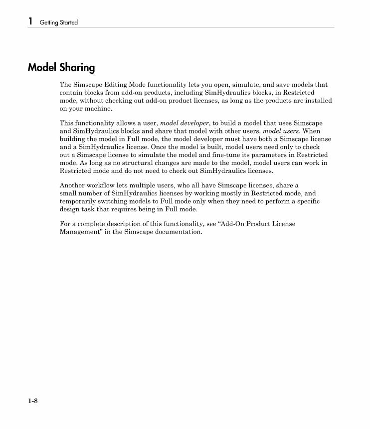
In our model, we have used the PS-Simulink Converter block in its default parameterconfiguration, which does not specify units. Therefore, the Position scope outputs thecylinder rod displacement in the units specified for the parameters of the Single-ActingHydraulic Cylinder block; in this case, in meters. This example shows how to change theoutput units for the cylinder rod displacement to millimeters.

1 Double-click the PS-Simulink Converter block. Type mm in the Output signal unittext box and click OK.

2 Run the simulation. In the Position scope window, click to autoscale the scopeaxes. The cylinder rod displacement is now output in millimeters, as shown in thefollowing illustration.


2-26

Modeling Power Units

2-27


The power unit is perhaps the most prevalent unit in hydraulic systems. Its mainfunction is to supply the required amount of fluid under specified pressure. There is awide variety of power unit designs varying by the amount and type of pumps, primemovers, valves, tanks, etc. The set of blocks available in the SimHydraulics librariesallows you to simulate practically any of these configurations. This section considersbasic approaches in simulating power units and examples of typical schematics.

A typical power unit of a hydraulic system, as shown in the following illustration,consists of a fixed-displacement or variable-displacement pump, reservoir, pressure-reliefvalve, and a prime mover that drives the hydraulic pump.

Typical Hydraulic Power Unit

In developing a model of a power unit, you must reach a compromise between therobustness, speed of simulation, and accuracy, meaning that the model should be assimple as possible to provide acceptable accuracy within the working range of variableparameters.

The first option is to simulate a power unit literally, as it is, reproducing all itscomponents. This approach is illustrated in the Power Unit with Fixed-DisplacementPump example. The power unit consists of a fixed-displacement pump, which is drivenby a motor through a compliant transmission, a pressure-relief valve, and a variableorifice, which simulates system fluid consumption. The motor model is represented as asource of angular velocity rotating shaft at 188 rad/s at zero torque. The load on the shaftdecreases the velocity with a slip coefficient of 1.2 (rad/s)/Nm. The load on the driving

../examples/power-unit-with-fixed-displacement-pump.html

../examples/power-unit-with-fixed-displacement-pump.html


2-28

shaft is measured with the torque sensor. The shaft between the motor and the pump isassumed to be compliant and simulated with rotational spring and damper.

The simulation starts with the variable orifice opened, which results in a low systempressure and the maximum flow rate going to the system. The orifice starts closing at0.5 s, and is closed completely at 3 s. The output pressure builds up until it reaches thepressure setting of the relief valve (75e5 Pa) and is maintained at this level by the valve.At 3 s, the variable orifice starts opening, thus returning system to its initial state.

You can implement a considerably more complex model of a prime mover by followingthe pattern used in the example. For instance, the shaft can be represented withmultiple segments and intermediate bearings. The model of a prime mover can be morecomprehensive, accounting for its type (DC or AC electric motor, diesel or gasolineengine), characteristics, control type, and so on. In addition, a complex mechanicaltransmission driven by a diesel or gasoline internal combustion engine modeled usingSimDriveline™ software can be combined with the SimHydraulics model of the hydraulicportion of a power unit.

Depending on your particular application, you may be able to simplify the model of apower unit practically without a loss in accuracy. The main factors to be considered inthis process are the driving shaft angular velocity variation magnitude and the systempressure variation range. If the prime mover angular velocity remains practicallyconstant during simulated time or varies insignificantly with respect to its steady-statevalue, the entire driving shaft subsystem can be replaced with the Ideal Angular VelocitySource block, whose output is set to the steady-state value, as it is shown in the followingillustration.


2-29

Using the Ideal Angular Velocity Source Block in Modeling Power Units

Furthermore, if pump delivery exceeds the system's fluid requirements at all times, thepump output pressure remains practically constant and close to the pressure settingof the pressure-relief valve. If this assumption is true and acceptable, the entire powerunit can be reduced to an ideal Hydraulic Pressure Source block, as shown in the nextillustration.


2-30

Using the Hydraulic Pressure Source Block in Modeling Power Units

The two previous examples demonstrate that the use of ideal sources is a powerful meansof reducing the complexity of models. However, you should exercise extreme cautionevery time you use an ideal source instead of a real pump. The substitution is possibleonly if there is an assurance that the controlled parameter (angular velocity in the firstexample, and pressure in the second example) remains constant. If this is not the case,the power unit represented with an ideal source will generate considerably more powerthan its simulated physical counterpart, thus making the simulation results incorrect.

Modeling Directional Valves

2-31


In this section...

“Types of Directional Valves” on page 2-31“4-Way Directional Valve Configurations” on page 2-32“Building Blocks and How to Use Them” on page 2-36“Build a Custom Directional Valve” on page 2-40

Types of Directional Valves

The main function of directional valves in hydraulic systems is to direct and distributeflow between consumers. As far as the valve modeling is concerned, the valves areclassified by the following main characteristics:

• Number of external paths (connecting ports) — One-way, two-way, three-way, four-way, multiple-way

• Number of positions a control member of the valve can assume — Two-position, three-position, multiple-position, continuous (can assume any position within workingrange)

• Control member type — Spool, poppet, sliding flat spool, and so on

As an example, the following illustration shows a portion of a hydraulic system witha 4-way, 3-position directional valve controlling a double-acting cylinder, next to itsschematic diagram.


2-32

Throughout SimHydraulics libraries, hydraulic ports are identified with the followingsymbols:

• P — Pressure port• T — Return (tank) port• A, B — Actuator ports• X, Y — Pilot or control ports

4-Way Directional Valve Configurations

4-way directional valves are available in multiple configurations, depending on theport connections in three distinctive valve positions: leftmost, neutral, and rightmost.Each configuration is characterized by the number of variable orifices, the way theorifices are connected, and initial openings of the orifices. Ten 4-way directional valveblocks in SimHydraulics libraries represent twenty most typical valve configurations.Configurations that differ only by the values of initial openings are covered by the samemodel.

The basic 4-Way Directional Valve block lets you model eleven most popularconfigurations by changing the initial openings of the orifices, as shown in the followingtable.

Basic 4-Way Directional Valve Configurations

No Configuration Initial Openings

1 All four orifices are overlapped in neutral position:

• Orifice P-A initial opening < 0• Orifice P-B initial opening < 0• Orifice A-T initial opening < 0• Orifice B-T initial opening < 0

2 All four orifices are open (underlapped) in neutral position:

• Orifice P-A initial opening > 0• Orifice P-B initial opening > 0• Orifice A-T initial opening > 0• Orifice B-T initial opening > 0


2-33


3 Orifices P-A and P-B are overlapped. Orifices A-T and B-Tare overlapped for more than valve stroke:

• Orifice P-A initial opening < 0• Orifice P-B initial opening < 0• Orifice A-T initial opening < – valve_stroke• Orifice B-T initial opening < – valve_stroke

4 Orifices P-A and P-B are overlapped, while orifices A-T andB-T are open:

• Orifice P-A initial opening < 0• Orifice P-B initial opening < 0• Orifice A-T initial opening > 0• Orifice B-T initial opening > 0

5 Orifices P-A and A-T are open in neutral position, whileorifices P-B and B-T are overlapped:

• Orifice P-A initial opening > 0• Orifice P-B initial opening < 0• Orifice A-T initial opening > 0• Orifice B-T initial opening < 0

6 Orifice A-T is initially open, while all three remaining orificesare overlapped:

• Orifice P-A initial opening < 0• Orifice P-B initial opening < 0• Orifice A-T initial opening > 0• Orifice B-T initial opening < 0

7 Orifice B-T is initially open, while all three remaining orificesare overlapped:

• Orifice P-A initial opening < 0• Orifice P-B initial opening < 0


2-34


• Orifice A-T initial opening < 0• Orifice B-T initial opening > 0

8 Orifices P-A and P-B are open, while orifices A-T and B-T areoverlapped:

• Orifice P-A initial opening > 0• Orifice P-B initial opening > 0• Orifice A-T initial opening < 0• Orifice B-T initial opening < 0

9 Orifice P-A is initially open, while all three remaining orificesare overlapped:

• Orifice P-A initial opening > 0• Orifice P-B initial opening < 0• Orifice A-T initial opening < 0• Orifice B-T initial opening < 0

10 Orifice P-B is initially open, while all three remaining orificesare overlapped:

• Orifice P-A initial opening < 0• Orifice P-B initial opening > 0• Orifice A-T initial opening < 0• Orifice B-T initial opening < 0

11 Orifices P-B and B-T are open, while orifices P-A and A-T areoverlapped:

• Orifice P-A initial opening < 0• Orifice P-B initial opening > 0• Orifice A-T initial opening < 0• Orifice B-T initial opening > 0

The other nine configurations are covered by the remaining 4-way directional valveblocks (A through K), as shown in the next table.


2-35

Other 4-Way Directional Valve Blocks

Block Name Configuration Description

4-Way Directional Valve A Contains two additionalnormally-open, sequentially-located orifices. Valvedisplacement to the left or tothe right closes the path totank.

4-Way Directional Valve B Ports P and A are permanentlyconnected through fixed orifice.Orifices P-B and B-T areinitially open (underlapped).

4-Way Directional Valve C Ports P and B are permanentlyconnected through fixed orifice.Orifices P-A, A-T and B-T areinitially open (underlapped).

4-Way Directional Valve D Two orifices are installed in theP-A link. Port A never connectsto port T.

4-Way Directional Valve E Two orifices are installed in theP-B link. Port B never connectsto port T.

4-Way Directional Valve F Two parallel orifices in the P-A arm and two series orifices inthe A-T arm.


2-36

Block Name Configuration Description

4-Way Directional Valve G Two parallel orifices in the P-B arm and two series orifices inthe B-T arm.

4-Way Directional Valve H Two parallel orifices in the P-B arm and two series orifices inthe P-T arm.

4-Way Directional Valve K Two parallel orifices in the P-A arm and two series orifices inthe P-T arm.

Building Blocks and How to Use Them

The Directional Valves library offers several prebuilt directional valve models. Asindicated in their descriptions, all of them are symmetrical, continuous valves. In otherwords, the control member in 2-way, 3-way, 4-way, and 6-way valves can assume anyposition, controlled by the physical signal port S. The valves are symmetrical in that allthe orifices the valve is built of are of the same type and size. The only possible differencebetween orifices is the orifice initial opening.

These configurations cover a substantial portion of real valves, but the directional valvesfamily is so diverse as to make it practically impossible to have a library model forevery member. Instead, SimHydraulics libraries offer a set of building blocks that iscomprehensive enough to build a model for any real configuration. This section describesthe rules of building a custom model of a directional valve.

All directional valve models are built of variable orifices. In SimHydraulics libraries, thefollowing variable orifice models are available:

• Annular Orifice• Orifice with Variable Area Round Holes


2-37

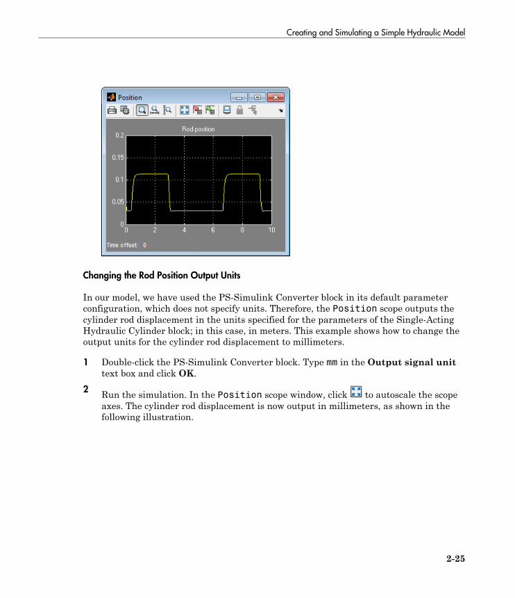
• Orifice with Variable Area Slot• Variable Orifice• Ball Valve• Ball Valve with Conical Seat• Needle Valve• Poppet Valve

To simplify the way variable orifices are combined in a model, their instantaneousopening is computed in the same way for all types of orifices. The orifice opening isalways computed in the direction the spool, or any other control member, opens theorifice. In other words, positive value of the opening corresponds to open orifice, whilenegative value denotes overlapped, or closed, orifice. The origin always corresponds tozero-lap position, when the edge of the control member coincides with the edge of theorifice. In the illustration below, origins are marked with 0 for the orifice with variablearea round holes (schematic on the left) and for the orifice with variable slot (schematicon the right). The x arrow denotes the direction in which orifice opening is measured inboth cases.

The instantaneous value of the orifice opening is determined as

h x x orsp= +0 i


2-38

where

h Instantaneous orifice opening.x0 Initial opening. The initial opening value is positive for initially open

(underlapped) orifices and negative for overlapped orifices.xsp Spool (or other control member) displacement from initial position, which

controls the orifice.or Orifice orientation indicator. The variable assumes +1 value if a spool

displacement in the globally assigned positive direction opens the orifice, and-1 if positive motion decreases the opening.

The number of variable orifices and the way they are connected are determined by thevalve design. Usually, the model of a valve mimics the physical layout of a real valve.The illustration below shows an example of a 4-way valve, its symbol, and an equivalentcircuit of its SimHydraulics model.


2-39

The 4-way valve in its simplest form is built of four variable orifices. In the equivalentcircuit, they are named P_A, P_B, A_T, and B_T. The Variable Orifice block, which isthe most generic model of a variable orifice in the SimHydraulics libraries, is used inthis particular example. You can use any other variable orifice blocks if the real valvedesign employs a configuration backed by a stock model, such as an orifice with roundholes or rectangular slots, poppet, ball, or needle. In general, all orifices in the modelcan be simulated with different blocks or with the same block, but with different way ofparameterization. For instance, two orifices can be represented by their pressure-flowcharacteristics, while two others can be simulated with the table-specified area variationoption (for details, see the Variable Orifice block reference page).

The next example shows another configuration of a 4-way directional valve. This valveunloads the pump in neutral position and requires six variable orifice blocks. The Orificewith Variable Area Round Holes blocks have been used as a variable orifice in this model.Port T1 corresponds to an intermediate point between ports P and T.


2-40

Build a Custom Directional Valve

Finally, let us consider a more complex directional valve example. The figure belowshows basic elements of a front loader hydraulic system. Both the lift and the tilt


2-41

cylinders are controlled by custom 3-position, 5-way valves, developed for this particularapplication. The valves are designed in such a way that the pump delivery is divertedto tank (unloaded) if both cylinders are commanded to be in neutral position. The pumpis disconnected from the tank if either of the two control valves is shifted from neutralposition.

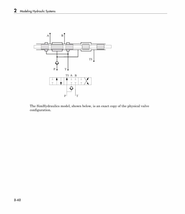
To develop a model, the physical version of the valve must be created first. The followingillustration shows one of the possible configurations of the valve.


2-42

The SimHydraulics model, shown below, is an exact copy of the physical valveconfiguration.


2-43

All the orifices in the model are closed (overlapped) in valve neutral position, exceptorifices P_T1_1 and P_T1_2. These two orifices should be set open to an extent thatallows pump delivery to be discharged at low pressure.


2-44

Modeling Low-Pressure Fluid Transportation Systems

In this section...

“How Fluid Transportation Systems Differ from Power and Control Systems” on page2-44“Available Blocks and How to Use Them ” on page 2-46“Low-Pressure Fluid Transportation System” on page 2-48

How Fluid Transportation Systems Differ from Power and Control Systems

In hydraulics, the steady uniform flow in a component with one entrance and one exit ischaracterized by the following energy equation

- =-

+-

+ - +

&

&

W

mg

V V

g

p p

gz z hs

L2

2

1

2

2 12 1

2 r

where

&Ws

Work rate performed by fluid

&m Mass flow rate

V2 Fluid velocity at the exitV1 Fluid velocity at the entrancep1, p2 Static pressure at the entrance and the exit, respectivelyg Gravity accelerationρ Fluid densityz1, z2 Elevation above a reference plane (datum) at the entrance and the exit,

respectivelyhL Hydraulic loss

Subscripts 1 and 2 refer to the entrance and exit, respectively. All the terms inEquation 2-1 have dimensions of height and are named kinematic head, piezometrichead, geometric head, and loss head, respectively. For a variety of reasons, analysis ofhydraulic power and control systems is performed with respect to pressures, rather thanto heads, and Equation 2-1 for a typical passive component is presented in the form


2-45

rr

rr

2 212

1 1 22

2 2V p gz V p gz pL+ + = + + +

where

V1, p1, z1 Velocity, static pressure, and elevation at the entrance, respectivelyV2, p2, z2 Velocity, static pressure, and elevation at the exit, respectivelypL Pressure loss

Term r

2

2V is frequently referred to as kinematic, or dynamic, pressure, and rgz as

piezometric pressure. Dynamic pressure terms are usually neglected because they arevery small, and Equation 2-2 takes the form

p gz p gz pL1 1 2 2+ = + +r r

The size of a typical power and control system is usually small and rarely exceeds 1.5– 2 m. To add to this, these systems operate at pressures in the range 50 – 300 bar.Therefore, rgz terms are negligibly small compared to static pressures. As a result,SimHydraulics components (with the exception of the ones designed specifically forlow-pressure simulation, described in “Available Blocks and How to Use Them ” onpage 2-46) have been developed with respect to static pressures, with the followingequations

p p f q

q f p p

L= =

=

( )

( , )1 2

where

p Pressure difference between component portsq Flow rate through the component

Fluid transportation systems usually operate at low pressures (about 2-4 bar), and thedifference in component elevation with respect to reference plane can be very large.Therefore, geometrical head becomes an essential part of the energy balance and mustbe accounted for. In other words, the low-pressure fluid transportation systems must


2-46

be simulated with respect to piezometric pressures p p gzpz = + r , rather than staticpressures. This requirement is reflected in the component equations

p p f q z z

q f p p z z

L= =

=

( , , )

( , , , )

1 2

1 2 1 2

Equations in the form Equation 2-5 must be applied to describe a hydraulic componentwith significant difference between port elevations. In hydraulic systems, there is onlyone type of such components: hydraulic pipes. The models of pipes intended to be usedin low pressure systems must account for difference in elevation of their ports. Thedimensions of the rest of the components are too small to contribute noticeably to energybalance, and their models can be built with the constant elevation assumption, like allthe other SimHydraulics blocks. To sum it up:

• You can build models of low-pressure systems with difference in elevations of theircomponents using regular SimHydraulics blocks, with the exception of the pipes. Uselow-pressure pipes, described in “Available Blocks and How to Use Them ” on page2-46 .

• When modeling low-pressure systems, you must use low-pressure pipe blocks toconnect all nodes with difference in elevation, because these are the only blocks thatprovide information about the vertical locations of the system parts. Nodes connectedwith any other blocks, such as valves, orifices, actuators, and so on, will be treated asif they have the same elevation.

Available Blocks and How to Use Them

When modeling low-pressure hydraulic systems, use the pipe blocks from the Low-Pressure Blocks library instead of the regular pipe blocks. These blocks account for theport elevation above reference plane and differ in the extent of idealization, just like theirhigh-pressure counterparts:

• Resistive Pipe LP — Models hydraulic pipe with circular and noncircular crosssections and accounts for friction loss only, similar to the Resistive Tube block,available in the Simscape Foundation library.

• Resistive Pipe LP with Variable Elevation — Models hydraulic pipe with circular andnoncircular cross sections and accounts for friction losses and variable port elevations.Use this block for low-pressure system simulation in which the pipe ends change theirpositions with respect to the reference plane.


2-47

• Hydraulic Pipe LP — Models hydraulic pipe with circular and noncircularcross sections and accounts for friction loss along the pipe length and for fluidcompressibility, similar to the Hydraulic Pipeline block in the Pipelines library.

• Hydraulic Pipe LP with Variable Elevation — Models hydraulic pipe with circularand noncircular cross sections and accounts for friction loss along the pipe length andfor fluid compressibility, as well as variable port elevations. Use this block for low-pressure system simulation in which the pipe ends change their positions with respectto the reference plane.

• Segmented Pipe LP — Models circular hydraulic pipe and accounts for friction loss,fluid compressibility, and fluid inertia, similar to the Segmented Pipe block in thePipelines library.

Use these low-pressure pipe blocks to connect all hydraulic nodes in your model withdifference in elevation, because these are the only blocks that provide information aboutthe vertical location of the ports. Nodes connected with any other blocks, such as valves,orifices, actuators, and so on, will be treated as if they have the same elevation.

The additional models of pressurized tanks available for low-pressure system simulationinclude:

• Constant Head Tank — Represents a pressurized hydraulic reservoir, in which fluidis stored under a specified pressure. The size of the tank is assumed to be largeenough to neglect the pressurization and fluid level change due to fluid volume. Theblock accounts for the fluid level elevation with respect to the tank bottom, as well asfor pressure loss in the connecting pipe that can be caused by a filter, fittings, or someother local resistance. The loss is specified with the pressure loss coefficient. The blockcomputes the volume of fluid in the tank and exports it outside through the physicalsignal port V.

• Variable Head Tank — Represents a pressurized hydraulic reservoir, in which fluidis stored under a specified pressure. The pressurization remains constant regardlessof volume change. The block accounts for the fluid level change caused by the volumevariation, as well as for pressure loss in the connecting pipe that can be caused by afilter, fittings, or some other local resistance. The loss is specified with the pressureloss coefficient. The block computes the volume of fluid in the tank and exports itoutside through the physical signal port V.

• Variable Head Two-Arm Tank — Represents a two-arm pressurized tank, in whichfluid is stored under a specified pressure. The pressurization remains constantregardless of volume change. The block accounts for the fluid level change caused bythe volume variation, as well as for pressure loss in the connecting pipes that can becaused by a filter, fittings, or some other local resistance. The loss is specified with the


2-48

pressure loss coefficient at each outlet. The block computes the volume of fluid in thetank and exports it outside through the physical signal port V.

• Variable Head Three-Arm Tank — Represents a three-arm pressurized tank, inwhich fluid is stored under a specified pressure. The pressurization remains constantregardless of volume change. The block accounts for the fluid level change caused bythe volume variation, as well as for pressure loss in the connecting pipes that can becaused by a filter, fittings, or some other local resistance. The loss is specified with thepressure loss coefficient at each outlet. The block computes the volume of fluid in thetank and exports it outside through the physical signal port V.

Low-Pressure Fluid Transportation System

The following illustration shows a simple system consisting of three tanks whose bottomsurfaces are located at heights H1, H2, and H3, respectively, from the reference plane.The tanks are connected by pipes to a hydraulic manifold, which may contain anyhydraulic elements, such as valves, orifices, pumps, accumulators, other pipes, and so on,but these elements have one feature in common – their elevations are all the same andequal to H4.


2-49

The models of tanks account for the fluid level heights F1, F2, and F3, respectively, andrepresent pressure at their bottoms as

p gF ii i= =r for 1 2 3, ,

The components inside the manifold can be simulated with regular SimHydraulicsblocks, like you would use for hydraulic power and control systems simulation. Thepipes must be simulated with one of the low-pressure pipe models: Resistive PipeLP, Hydraulic Pipe LP, or Segmented Pipe LP, depending on the required extent ofidealization. Use the Constant Head Tank or Variable Head Tank blocks to simulatethe tanks. For details of implementation, see the Water Supply System and the FluidTransportation System with Three Tanks examples.

../examples/water-supply-system.html

../examples/fluid-transportation-system-with-three-tanks.html

../examples/fluid-transportation-system-with-three-tanks.html

simhydraulics user's guide - dphu · directions; directional valves bypassed by a huge...

Documents