Simulating Correlated Defaults

Darrell DuÆe and Kenneth Singleton�

May 21, 1999

Graduate School of Business, Stanford University

Abstract: This paper reviews some conventional and novel approachesto modeling and simulating correlated default times (and losses) on portfoliosof loans, bonds, OTC derivatives, and other credit positions. We emphasizethe impact of correlated jumps in credit quality on the performance of largeportfolios of positions.

�DuÆe is with the Graduate School of Business, Stanford University, Stanford, CA94305, duÆe@baht.stanford.edu. Singleton is with the Graduate School of Business,Stanford University, Stanford, CA 94305 and NBER, kenneths@future.stanford.edu. Ourbiggest acknowledgement is to Jun Pan for exceptional research assistance. We are grate-ful for conversations with Josh Danziger of CIBC and David Lando, and for motivat-ing discussions with Gi�ord Fong of Gi�ord Fong Associates and Jim Vinci of Price-WaterhouseCoopers. This work is supported by PriceWaterhousCoopers Risk Insti-tute, of which the authors are members, and by the Gi�ord Fong Associates Fund atthe Graduate School of Business, Stanford University. The paper is downloadable athttp://www-leland.stanford.edu/�duffie/.

1

Contents

1 Introduction 3

2 Economic Framework 5

3 Multi-Entity Default Intensity 8

3.1 Constant and Independent Default Risk . . . . . . . . . . . . 83.2 Joint Credit Events . . . . . . . . . . . . . . . . . . . . . . . . 93.3 Example: Multivariate-Exponential Default Times . . . . . . . 11

4 Default Time Simulation Algorithms 12

4.1 Single-Entity Default Time Simulation . . . . . . . . . . . . . 124.2 Multi-Entity Default Time Simulation . . . . . . . . . . . . . 13

5 Conventional Stochastic Intensity Models 15

5.1 Di�usion Intensities . . . . . . . . . . . . . . . . . . . . . . . . 165.2 Finite-State Continuous-time Markov Chains . . . . . . . . . . 175.3 HJM Forward Default Probabilities . . . . . . . . . . . . . . . 17

6 Correlated Jump Intensity Processes 18

6.1 Mean-Reverting Intensities with Jumps . . . . . . . . . . . . . 186.2 Correlated Jump Intensity Processes . . . . . . . . . . . . . . 226.3 Numerical Example . . . . . . . . . . . . . . . . . . . . . . . . 23

7 Correlated Log-Normal Intensities 29

7.1 Numerical Example . . . . . . . . . . . . . . . . . . . . . . . . 297.2 Check on Sampling Error . . . . . . . . . . . . . . . . . . . . . 307.3 Check on Time-Discretization \Error" . . . . . . . . . . . . . 307.4 Role of Intensity Volatility and Correlation . . . . . . . . . . . 32

A Review of Intensity Modeling 37

A.1 Poisson Arrival . . . . . . . . . . . . . . . . . . . . . . . . . . 37A.2 Intensity Process . . . . . . . . . . . . . . . . . . . . . . . . . 38A.3 Multivariate Exponential Event Times . . . . . . . . . . . . . 39

B More on the Jump Intensity Model 40

C More on the Log-Normal Intensity Model 42

2

1 Introduction

Computationally eÆcient methods for simulating default times for positionswith numerous counterparties are central to the credit risk-management andderivative-pricing systems of major �nancial institutions. The likelihood ofdefault of a given counterparty or borrower in a given time period is typicallysmall. Computing the distribution of default times or losses on a large port-folio to reasonable accuracy may therefore require a signi�cant number ofsimulated scenarios. This paper describes several computationally eÆcientframeworks for simulating default times for portfolios of loans and OTCderivatives, and compares some of the features of their implied distributionsof default times.

Our focus is on the simulation of correlated credit-event times, whichwe can treat for concreteness as the default times of a given list of entities,such as corporations, private borrowers, or sovereign borrowers. To put thecomputational burden of a typical risk-management problem in perspective,consider a hypothetical portfolio consisting of 1,000 randomly selected �rmsrated Baa by Moody's, and suppose the risk manager is interested in 10-year scenarios. As indicated by the average default rates for 1970-97 inFigure 1, Baa �rms experienced default at a rate of 0.12% per year, onaverage, over this period. Our sample portfolio of 1,000 Baa �rms wouldthus have experienced a total average rate of approximately 12 defaults peryear over this period. A \brute-force" simulation of default times for theportfolio using, say, weekly survival-default simulation would call for 10 �52 � 1000 = 0:52 million survive-or-default draws per 10-year scenario forthis portfolio. One also must update, week by week, the conditional defaultprobabilities of each entity, for another 0.52 million draws. Given randomvariation in exposures at default, we �nd that an order of magnitude ofroughly 10,000 independent scenarios may be appropriate for estimation of\long-tail" con�dence levels on total default losses for this sort of portfolio.(Reduction in the computational burden would likely come from variance-reduction or importance-sampling methods.) Simulation of 10,000 scenariosby the brute-force approach would thus call for on the 10 billion of survive-or-default random draws for each set of model parameters. In order to conductstress testing calibration, many such exercises may be called for.

Fortunately such computationally intensive algorithms are unnecessaryfor many risk-management and pricing applications. Instead, one can use avariant of the following basic recursive event-time simulation algorithm for

3

Source: Moody's 1998

AverageDefaultRate(basispoints)

0

100

200

300

400

500

600

700

Aaa Aa A Baa Ba B

0bps

0bps

1bps

3bps

9bps

9bps

12bps

32bps

146bps

134bps

442bps

678bps

1920-19971970-1997

Figure 1: One year, weighted-average default rates by Moody's rating.

generating random multi-year scenarios for default times on a portfolio:

1. Given the simulated history to the last default time Tk, simulate thenext time Tk+1 of default of any entity. If Tk+1 is after the lifetime ofthe portfolio, stop.

2. Otherwise, simulate the identities of any entities defaulting at Tk+1, aswell as any other variables necessary to update the simulation modelfor the next default time.

3. Replace k with k + 1, and go back to Step 1.

Algorithms based on recursive event-time simulation are relatively eÆcientfor large portfolios of moderate or low credit risk. For our hypothetical port-folio of 1,000 Baa counterparties, ignoring migration of credit quality for

4

the moment, the recursive event-time algorithm would call for an averageof about 12 random inter-default-time draws, and 12 draws for the identi-ties of the defaulting entities, per 10-year scenario. We will present severalframeworks that allow for random variation in an entity's credit-quality overtime, while still allowing for the basic eÆciency of the recursive event-timesimulation algorithm. Moreover, recursive event-time simulation accommo-dates correlation among default times, including correlations caused by creditevents that induce simultaneous jumps in the expected arrival rates of defaultof di�erent counterparties.

For bank-wide risk management decisions, one may be interested in thelikelihood that there will exist some interval of a given length, say 10 days,within the given multi-year planning horizon, during which default losses ex-ceed a given amount of a bank's capital. This could be useful information,for example, in setting the bank's capital, structuring its portfolio for liquid-ity, or setting up provisional lines of credit. For accuracy in this calculation,it would be necessary to simulate the default times of the di�erent entitiesto within relatively �ne time slots, say daily.1 Under the obvious provisothat the underlying probabilistic model of correlated default times is appro-priate, we show that the recursive event-time algorithm is also well suitedfor this task, as it generates the precise default times implied by the model,scenario by scenario. When implemented for some hypothetical portfolios,we �nd that such measures as the distribution of losses for the \worst twoweeks within 10 years" are particularly sensitive to one's assumption aboutcorrelation among entities.

2 Economic Framework

Throughout this analysis, we take as given a formulation of the default prob-abilities of each of the counterparties. We remain agnostic about the natureof the economic information driving default and the structural model linkingthis information to the default event. By way of background, we begin bypresenting a brief discussion of the frameworks that one might consider when

1For example, given a loss on a certain day, a subsequent loss 11 days later should notenter the associated 10-day loss window, whereas a loss 9 days later should. If one is onlyinterested in measures of default losses over �xed accounting periods, say quarterly, thenthe compuational burden of the brute-force simulation approach can be reduced somewhatby moving from daily to perhaps quarterly frequency for survival-default random draws.

5

modeling default events.For corporate entities, foundational research on corporate debt pricing

by Black and Scholes (1973) and Merton (1974) suggests modeling defaultprobabilities at a given horizon as the likelihood that assets will not be suf-�cient to meet liabilities. Important variants and extenstions of the modelallowing treatment of term-structures include those due to Geske (1977), Le-land (1994), Leland and Toft (1996), and Longsta� and Schwartz (1995).This class of models is the theoretical underpinnings of the popular commer-cial \EDF" measure of default probability supplied by KMV Corporation.2

That it has predictive power for rating migrations and defaults is shown, forexample, by Delianedis and Geske (1998).

As far as implementation of this corporate-�nance framework for pur-poses of simulating correlated default times for a list of �rms, at least twomethodologies are feasible:

A. Simulate the underlying asset processes until \�rst-passage" of assetsto default boundaries, as follows:

(a) From equity or bond (or both) price data, �t correlation andvolatility parameters of log-asset-value processes, modeled, say,as Brownian motions.

(b) Fit, as well, boundaries, possibly time dependent, that determinethe default time of each �rm as the �rst time that its assets crossits default boundary.

(c) Simulate the sample paths of the underlying correlated Brownianmotions, and record the �rst passage times for each �rm.

B. The \intensity" of default for a given �rm is the conditional expectedarrival rate of default, which may depend on many observables. (Aconstant intensity implies a \Poisson arrival" of default.) One can �tstochastic default-intensity models to publicly traded borrowers, frommarket data on equity and bond prices, and perhaps other data such astransition histories or macroeconomic business-cycle variables.3 Then

2See Kealhofer (1995).3For example, Wilson (1997) proposes to �t transition intensities to country-level eco-

nomic performance measures. This implies independence of default times for within-country entities, conditional on domestic business-cycle variables. One could model cor-relation induced by industry performance by a similar mechanism.

6

simulate correlated default times using well known algorithms, somereviewed below, for simulation of stopping times with given intensities.

A special case of the intensity-based Approach B is the CreditMetricsmodel of JP Morgan, for which one �ts a model of credit-rating transitions,with correlations in rating changes that are implied by estimated correlationsin changes in �rm values. In e�ect, the default-time distribution for a given�rm is based on historical rating transition and default data, while corre-lations in ratings changes can be \calibrated" to market cross-�rm equityreturn correlations.4

In principle, Approaches A and B both allow one to use information aboutthe prices of corporate securities when �tting a default-timing model. Use ofthis information seems desirable, because:

� Equity and corporate bond prices re ect market views of both assetvaluations as well as asset volatilities. For individual entities, thisprovides enough information, in the context of the model, to derive\risk-neutral" default probabilities. Time-series data may supply riskpremia with which one could estimate intensities.

� Correlation in the timing of default among di�erent entities can beinferred through the model.

For the �rst-passage simulation method, Approach A, simulation of thepaths of asset levels until �rst passage to default boundaries is burdensomefor a large number of entities over long time horizons. Moreover, for longtime horizons, it is not obvious how to control this simulation method forrealistic re-capitalization possibilities. Calibration to reasonable long-termdefault probabilities may be intractable, if not unrealistic.

In the remainder of this paper, we focus on default-time simulation us-ing Approach B, based on various models of default-arrival intensities. We

4The algorithm is roughly as follows: (i) Estimate the correlations of the variousentities asset re-valuations, based on historical equity returns. (ii) For each entity, choosevarious levels of asset returns as cuto� boundaries for ratings or default so as to matchthe desired (say, historically estimated) rating transition probabilities. See, for example,Introduction to Credit Metrics, J.P. Morgan, New York, April 1997, page 26. By scalingarguments, volatilities are irrelevant given transition probabilities, unless one incorporatesmean-return e�ects. (iii) Simulate a joint Gaussian vector for asset returns of all entities,and allocate the entities to their new ratings, or default, based on the outcomes.

7

emphasize, however, that to the extent permitted by the data, it is advan-tageous to �t the model of stochastic intensities of the entities to marketequity or bond price behavior, economy-wide business cycle data, industryperformance data, and the historical timing of ratings and default. Bijnenand Wijn (1994), Lennox (1998), Lundstedt (1999), McDonald and Van deGucht (1996), and Shumway (1997) provide some examples. Intensity-basedsimulation is consistent in theory with �rst-passage simulation. For exam-ple, DuÆe and Lando (1998) present a simple model in which, because ofimperfect observation of a �rm's assets (or the default boundary), there is adefault intensity that can be estimated from asset reports.

3 Multi-Entity Default Intensity

This section reviews the basic ideas of intensity modeling for multi-entityportfolios. Appendix A reviews the more primitive underlying single-entityintensity model.

Throughout, we use the fact that the sum N = Nr +NR of independentPoisson arrival processes Nr and NR, with respective intensities r and R,is itself a Poisson process with intensity r + R. The same property applieswith randomly varying arrival intensities, under certain conditions, the mostcritical of which is that the arrivals cannot occur simultaneously. With si-multaneous default, one can instead formulate separate credit events thatcould cause more than one entity to default at the same time, and to modelthe intensity of such joint credit events, as we shall see.

3.1 Constant and Independent Default Risk

Suppose, for illustration, that there are nA counterparties of type A, eachwith default at intensity hA, and nB of type B, each with default intensity hB.The time horizon T is �xed for this discussion. The intensities are assumedto be constant. We assume, for now, that two �rms cannot default at thesame time. In this case, we can simulate the defaulting �rms, and timesof their defaults, by the following simple version of the recursive event-timealgorithm.

1. We �rst simulate a single Poisson process up to time T , with intensityH = hAnA + hBnB. For example, with nA = 1000 A-rated counterpar-ties, each with default intensities of hA = 0:001 per year, and nB = 100

8

B-rated counterparties, each with with an intensity of hB = 0:05 peryear, we have a total intensity of H = 1 + 5 = 6 defaults per year.The inter-arrival times T1, and Ti � Ti�1, for i > 0, are simulated asindependent exponentially distributed variables of parameter H, andsuccessively added together to get the times T1; T2, : : : . This gives usthe default times and the number of �rms defaulting before T .

2. At each default time Ti, the �rm to default is of type A with probabilitya = nAhA=(nAhA + nBhB), and is of type B with probability 1 �a. We draw a random variable Y , called a \Bernoulli trial," whoseonly outcomes are A and B, with P (Y = A) = 1 � P (Y = B) =a. If the outcome of Y is A, we select one of the remaining type-A�rms to default at time Ti, at random. (That is, each �rm is drawnwith probability 1=nA.) If the outcome of Y is B, we draw one of theremaining type-B �rms, again at random.

3. We could adjust the arrival rates of default events of each type as �rmsdefault or otherwise disappear. This nuisance can be avoided simplyby \not counting" �rms that have already defaulted once. For someportfolios, such as revolving portfolios of bonds or loans underlyingcollateralized debt obligations, one can accomodate the introductionof new entities over time based on the simulated performance of theportfolio to date as well as simulated market data such as interest rates.One could extend the contagion model of Davis (1999) by modeling ajump in the default intensity of one entity with the default by someother entity.

In this way, we obtain, for each scenario, a list of the counterparties thatdefault and times at which each defaults. Because, typically, only a smallfraction of counterparties default in a given simulated scenario, this may bean eÆcient computational method for simulating total default losses. Rela-tively few market values and netting e�ects need to be computed.

3.2 Joint Credit Events

Certain credit events may be common to a number of counterparties. Thesecould include:

� Severe catastrophes (for example, \Earthquake in Tokyo").

9

� Systemic default or liquidity breakdowns.

� Sovereign risks, such as a default, a moratorium on capital out ows, ora devaluation.

� Counterparties linked to each other through contracts or capital struc-ture.

With joint credit events, some of the default intensity of each entity istied to an event at which any entity may default, with some given probability.The total default intensity of entity i at time t is

hit = pitJt +Hit;

where, at time t,

� Jt is the intensity for arrival of joint credit events.

� pit is the probability that entity i defaults given a joint credit event.

� Hit is the intensity of arrival of default speci�c to entity i.

With this model, the intensity of arrival of any kind of event is

Ht = Jt +H1t + � � �+Hnt:

In order to simulate defaults, one can adopt the following variant of therecursive event-time algorithm, which allows for correlation both through cor-related changes in default intensities, as well as through joint credit events.For now, we will assume that default intensities are changing deterministi-cally between defaults and credit events. Later, we allow them to be generalcorrelated random processes, subject to technical conditions and of coursethe tractability necessary to apply our general algorithmic approach.

1. Generate the next credit event time t, conditional on current informa-tion, based on the total intensity process H. If t > T , stop.

2. At the event time t, allocate the event, as joint, with probability,pJ(t) = Jt=(Jt+H1t+� � �+Hnt); or not joint, with probability 1�pJ(t).

10

3. If the type of event is simulated to be joint, then survive-or-defaultdraws are simulated for each entity, independently or with correlation,depending on the model speci�cation, entity i defaulting with proba-bility pit.

4. If the simulated event is not joint, then one of the counterpartiesis drawn at random to default. Entity i is drawn with probabilityHit=(H1t + � � �+Hnt):

5. Any defaulting counterparties are deleted from the list.

6. According to the model speci�cation, the intensity processesH1; : : : ; Hn; Jand event-conditional default probabilities p1; : : : ; pn are reset, condi-tioning on the history to date, and one returns to Step 1.

In the simplest version of the model, the only adjustment of intensities in thelast step is to replace the intensity process Hi and event-conditional defaultprobability pi of any defaulting entity with zeros. More general versions arediscussed below.

3.3 Example: Multivariate-Exponential Default Times

A special case of this approach is the classical multivariate-exponential dis-tribution of failure times, reviewed in Appendix A, under which all individualintensities (Hi and J) and conditional default probabilities (pi) are constant.In this case, each entity's default time is literally a Poisson arrival.

The main advantage of the multivariate exponential model is its sim-plicity. Simulation is easy. Numerous statistics (moments, joint survivalprobabilities, and so on) are easily calculated explicitly. For example, for�rst-to-default swap pricing, the impact of correlation is easily captured.

On the other hand, the model is not easily calibrated to data that bearon the term structure of default probabilities, such as bond or equity pricedata. For example, with risk-neutral bond investors, the term structure ofcredit yield spreads for the multivariate exponential model of default timesis literally at, because the default hazard rates are constant, whereas creditspreads often exhibit substantial slope, volatility, and correlation. (Term-structure e�ects could also be in uenced by time-variation in conditionalexpected recoveries at default, as in Das and Tufano (1996), or in risk pre-mia.)

11

Moreover, it is somewhat unrealistic to suppose that two or more �rmswould default literally simultaneously, unless there is a parent-subsidiary orsimilar contractual relationship. While the di�erence between simultaneousand nearly-timed default may not be critical for expected default losses orfor the pricing of certain credit derivatives, it may indeed be an importantdistinction for measurement of the likelihood of a given sized loss within agiven time window. With the multivariate exponential model, to the extentthat correlations in the incidence of defaults within a given year are realisti-cally captured, the model may imply an unrealistic amount of default withina given week or month.

4 Default Time Simulation Algorithms

Given stochastic intensity processes h1; : : : ; hn for each entity, our objectiveis to simulate the associated default times �1; : : : ; �n, as well as the identitiesof the defaulter at each default time. Two of the basic algorithms, comingfrom the reliability literature on failure-time modeling,5 are reviewed below.In some cases, as we shall point out, these algorithms are computationallyburdensome for general correlated multi-variate di�usion models for intensi-ties. In later sections, we suggest some tractable models.

4.1 Single-Entity Default Time Simulation

The primitive for the single-entity case is a stochastic intensity process h fora default time � . As a �rst step, it is helpful if one can tractably compute,at any time t before default, the conditional probability p(t; s) of survivalto any given time s > t. Under certain conditions, the conditional survivalprobability p(t; s) is given by

qt(s) = Et

�exp

�Z t

0

�h(s) ds

��; (1)

where Et denotes conditional expectation given the information available attime t. A key condition6 for this result is that, for the �xed time horizon s,the process fqs(t) : t � 0g de�ned by (1) does not jump at � . For example,

5See, for example, the survey by Shaked and Shanthikumar (1993).6For more on this condition, see DuÆe, Schroder, and Skiadas (1996). Kusuoka (1998)

provides some interesting examples in which this condition fails.

12

it is enough that h is a di�usion process, or a jump di�usion with jump timesthat are not default times. We would want a model for h allowing qt(s) to beeasily computed. Several such models are discussed in the following section.

In any case, there are two well known algorithms for simulation of thedefault time � :

(A) Inverse-CDF Simulation: Build a model in which the survival prob-ability p(0; t) is easily calculated. Simulate a uniformly distributedrandom variable U , and let � be chosen7 so that p(0; �) = U .

(B) Compensator Simulation: Build a model in which the accumu-lated intensity, H(t) =

R t

0h(u) du, often called the \compensator," is

feasibly simulated. Simulate, independently of H, a standard (unitmean) exponentially distributed variable Z. Let � be chosen8 so thatH(�) = Z.

Compensator simulation can be intractable unless the compensator can beeasily simulated. For di�usion models of intensity, exact compensator simula-tion is relatively computationally intensive if the sample paths of the underly-ing di�usion must be simulated. One could use Euler or higher-order schemesfor discrete-time approximate simulation of the stochastic di�erential equa-tions underlying the intensities. Depending on the number of discrete timeperiods and the number of scenarios, this may be relatively expensive.

4.2 Multi-Entity Default Time Simulation

Suppose the event times �1; : : : ; �n have respective intensity processes h1; : : : ; hn.For simplicity, simultaneous default is ruled out. (That is, the probabilitythat �i = �j is assumed to be zero for i 6= j. Otherwise, one reduces tosimulation of the underlying event times at which simultaneous default mayoccur.)

One can simulate the times �1; : : : ; �n with the correct joint distribution(including correlation of course) by either of the following basic algorithms,letting T denote the time horizon, assuming that one is interested in knowingthe outcome of �i only if it is in the interval (0; T ).

7This assumes that p(0; t) ! 0 as t ! 1. If not, then let � = infft : p(0; t) � Ug,which may have +1 as an outcome.

8This assumes that H(t)!1 as t!1. If not, then let � = infft : H(t) � Zg, whichmay have +1 as an outcome.

13

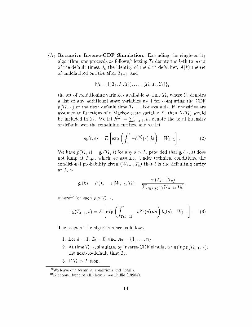
(A) Recursive Inverse-CDF Simulation: Extending the single-entityalgorithm, one proceeds as follows,9 letting Tk denote the k-th to occurof the default times, Ik the identity of the k-th defaulter, A(k) the setof undefaulted entities after Tk�1, and

Wk = f(T1; I1; Y1); : : : ; (Tk; Ik; Yk)g;

the set of conditioning variables available at time Tk, where Yk denotesa list of any additional state variables used for computing the CDFp(Tk; � ) of the next default time Tk+1. For example, if intensities areassumed to functions of a Markov state variable X, then X(Tk) wouldbe included in Yk. We let h(k) =

Pi2A(k) hi denote the total intensity

of default over the remaining entities, and we let

qk(t; s) = E

�exp

�Z s

t

�h(k)(s) ds

� ���� Wk�1

�: (2)

We have p(Tk; s) = qk(Tk; s) for any s > Tk provided that qk( � ; s) doesnot jump at Tk+1, which we assume. Under technical conditions, theconditional probability given (Wk�1; Tk) that i is the defaulting entityat Tk is

gi(k) = P (Ik = i jWk�1; Tk) = i(Tk�1; Tk)P

j2A(k) j(Tk�1; Tk);

where10 for each s > Tk�1,

i(Tk�1; s) = E

�exp

�Z s

T (k�1)

�h(k)(u) du

�hi(s)

���� Wk�1

�: (3)

The steps of the algorithm are as follows.

1. Let k = 1, T0 = 0, and A0 = f1; : : : ; ng.

2. At time Tk�1, simulate, by inverse-CDF simulation using p(Tk�1; � ),the next-to-default time Tk:

3. If Tk > T stop.

9We leave out technical conditions and details.10For more, but not all, details, see DuÆe (1998a).

14

4. Simulate the identity Ik of the k-th defaulter from A(k), with theconditional probability that Ik = i equal to gi(k).

5. Simulate the additional \state" variables Yk, with their distribu-tion given the conditioning variables Wk�1; Tk; Ik.

6. Remove Ik from A(k � 1) to get A(k), and unless A(k) is empty,advance k by 1, and go back to Step 2.

(B) Multi-Compensator Simulation: Under technical conditions, thefollowing algorithm generates stopping times11 �1; : : : ; �n with the givenintensity processes h1; : : : ; hn. It is assumed that the compensatorHi(t) =

R t0hi(u) du can be simulated for each i and t.

(a) Simulate n independent unit-mean exponentially distributed ran-dom variables Z1; : : : ; Zn.

(b) For each i, if Hi(T ) < Zi, then �i > T:

(c) Otherwise, let �i = minft : Hi(t) = Zig:

The compensator simulation approach is also possible, in a more com-plicated form, if one computes the intensities when conditioning only thehistory of the default times and identities of defaulting entities. This in-formation structure is sometimes called the \internal �ltration," and theresulting intensities in this setting are often called conditional hazard rates.The failure-time simulation is then called the \multivariate hazard construc-tion," proposed12 by Norros (1986) and Shaked and Shanthikumar (1987).The multivariate-hazard construction is preferred if the hazard rates relativeto the internal �ltration can be computed explictly.

For our numerical results in later sections, we use recursive inverse-CDFsimulation.

5 Conventional Stochastic Intensity Models

A wide range of models of stochastic intensity processes with a signi�cantlevel of analytical tractability have been used for modeling individual default

11There is no claim of uniqueness. Uniqueness in distribution is however implied if oneassumes that, conditional on the paths of the intensities h1; : : : ; hn, the stopping times�1; : : : ; �n are independent.

12This is based on a result of Meyer (1971).

15

times. We will brie y consider some of these. We later propose some alterna-tive models that are relatively simple and tractable for correlated default-timesimulation. As we shall see, they have rather di�erent implications for theimpact of correlation.

We note the helpful analogy between survival probabilities and discountfunctions, as it is apparent from (1) that, for risk-neutral bond investors, qt(s)is mathematically equivalent, under technical conditions, to a zero-couponbond price at time t, for maturity s, at short interest rate h. This suggestsconvenient classes of intensity processes that have already been used to modelinterest rates.

5.1 Di�usion Intensities

A convenient di�usion model of intensities would take hi(t) = fi(Xt), forsome state-space process X of a simple, say Cox-Ingersoll-Ross (1985) (CIR)or more generally aÆne,13 form. Because the \discount" qt(s) is explicit forthis family of models, provided fi is itself aÆne, it is simple to simulate in-dividual entity default times. One can likewise simulate the �rst-to-defaulttime T1 = min(�1; : : : ; �n) by the inverse-CDF method as the CDF of T1is easily computed.14 In order to simulate subsequent chronologically or-dered default times T2; T3; : : : , there are di�erent approaches. For example,suppose T1 and the �rst entity I1 to default have been simulated as in therecursive inverse-CDF algorithm above. In order to simulate T2, the seconddefault time, one could �rst simulate the state vector X(T1) determining in-tensities at time T1, and then given X(T1), compute the new CDF p(T1; � )for the second default time T2, and so on. The conditional distribution ofX(T1) given (T1; I1) can be computed easily for CIR models15 although itneed not be easily simulated in multivariate CIR cases. Compensator simu-lation is feasible through simulation of the sample paths of X, but may becomputationally intensive. One could alternatively undertake compensatorsimulation using the multivariate hazard construction, that is, with respectto the internal �ltration, although the detailed hazard-rate calculations havenot yet been worked out for non-trivial cases beyond the CIR model, to ourknowledge.

13See DuÆe and Kan (1996).14See, for example, DuÆe (1998a).15See DuÆe (1998a).

16

5.2 Finite-State Continuous-time Markov Chains

Jarrow, Lando, and Turnbull (1996) proposed the use of �nite-state continuous-time Markov chains as a model of intensities, for purposes of term-structuremodeling for defaultable bonds. They identi�ed states with credit ratings.Arvanitis, Gregory, and Laurent (1998), Lando (1998b), Li (1998), Nakazato(1998), and Tepla (1999) have extended the model to allow stochastic varia-tion of intensities within rating.

As for multi-entity correlated rating-transition models, Lando (1998a)considered correlation within the framework of �nite-state continuous-timeMarkov chains for each entity's intensity, by taking each of the states tocorrespond to a particular list of ratings, by entity. For example, with 2entities and 3 ratings, A;B; and C, the states are

fAA;AB;AC;BA;BB;BC;CA;CB;CCg;

where, for example, AB is the state for which entity 1 is currently in ratingA and entity 2 is in rating B. This leads to an exponential growth in thesize of the state space as the number of entities and ratings grow.

For a more tractable version of this approach, one could assume symmetryconditions among entities, and that transition times for all entities within onerating to any other particular rating or default are multivariate exponential.Given the �rst time of a default or transition out of a particular rating,symmetry calls for drawing the identity of the defaulting or transitioningentities by picking at random, equally likely, some entity currently in thatrating. One then re-sets the total-intensity model for various transitions,draws another transitition time, and so on. A typical element of the statespace is simply a list consisting of the number of entities in each rating.16

5.3 HJM Forward Default Probabilities

One can formulate Heath-Jarrow-Morton (1992) (HJM) style models of theterm structure of survival probabilities, by again exploiting the analogy be-tween bond prices and survival probabilities. One formulates the conditionalprobability at time t of survival to time s as the process

p(t; s) = exp

��

Z s

t

f(t; u) du

�; (4)

16The state space is f1; : : : ; ngK , where n is the number of entities and K is the numberof ratings.

17

where for each �xed s, one supposes that f( � ; s) is an Ito process. One canadd the jumps to the formulation of f . From the model speci�ed for f , andthe HJM \drift" restriction17 imposed on f by the fact that fp(t; s) : t � 0gis a martingale, one obtains indirectly a stochastic model for the intensityprocess h(t) = f(t; t). The default time � can then by simulated, for exampleby inverse-CDF or compensator simulation.

HJM-style models of survival probabilities could be used to simulate cor-related default times for the various entities by compensator simulation, al-though this may be compuationally burdensome.

6 Correlated Jump Intensity Processes

One example that we have explored is a model in which individual entitieshave default intensities that mean revert, with correlated Poisson arrivals ofrandomly sized jumps. By formulating the individual-entity default intensityjump times as multivariate exponential, one arrives at a relatively simple butuseful model for simulating correlated defaults.

6.1 Mean-Reverting Intensities with Jumps

First we formulate a single entity's intensity process as a mean-revertingprocess with jumps. Speci�cally, the intensity process h of a typical entity'sdefault time has independently distributed jumps that arrive at some con-stant intensity �, and otherwise h mean reverts at rate k to a constant �. Asample path for such an entity, su�ering 4 modest jumps to its intensity, isillustrated in Figure 2. For this illustration, and our examples to follow, themean-reversion rate is k = 0:5. One can easily generalize.

With this simple model, the default arrival intensity h(t) of the default

17Suppose, for each �xed s, that df(t; s) = �(t; s) dt+�(t; s) dBt, where B is a standardBrownian motion in Rd and � and � satisfy certain measurability and integrability con-ditions. Then, under additional technical conditions, the martingale property of p( � ; s)implies that �(t; s) = �(t; s) �

R st�(t; u) du, for t � s. This is often called the \HJM drift

restriction." See Heath, Jarrow, and Morton (1992) for the drift restriction on f , givenits volatilities, and DuÆe (1998b) for more details on the application to default risk. It isliterally the case that f(t; s) is the hazard rate for default at s, conditional on informationat t. Simulation of f therefore makes for easy updates of conditional survival probabilies.

18

Year

DefaultIntensityh(basispoints)

2 4 6 8 10 1200

2

4

6

8

10

12

14

Figure 2: A simulated path of default intensity.

time � , in between jump events, satis�es the ordinary di�erential equation

dh(t)

dt= k(� � h(t)): (5)

Thus, at any time t between jump times, we have a simple solution

ht = � + e�k(t�T )(hT � �); (6)

where T is the time of the last jump and hT is the post-jump intensity attime T .

For example, suppose that jumps in intensity are exponentially distributedwith mean J . The initial condition h(0) and the parameters (k; �; J; �) de-termine the probability distribution of the default time. In fact, it can be

19

shown18 that the conditional probability at any t < � of survival from t to sis

p(t; s) = e�(s�t)+�(s�t)h(t); (7)

where

�(t) = �1�e�kt

k

�(t) = ���t� 1�e�kt

k

�� �

J+k

�Jt� ln

�1 + 1�e�kt

kJ��

:

For example, suppose � = 0:001, k = 0:5, � = 0:001, J = 5, and h(0) =0:001, meaning an initial mean arrival rate of default of once per thousandyears (10 basis points). For comparison, the average rate of default arrivalfor both A-rated and Aa-rated corporate issuers from 1920 to 1997 was 9basis points, according to Moody's,19 as illustrated in Figure 1.

At these parameters, a jump in default risk is likely to be devastating, asa mean jump in intensity of 5 implies a mean expected remaining life of lessthat 3 months. This model is slightly less risky20 than one in which an issuerdefaults at a constant intensity of 20 basis points. (For reference, the averagedefault arrival rate for all Baa-rated corporate issuers for 1920 to 1997, asmeasured by Moody's, is 32 basis points, as indicated in Figure 1.)

So-called \risk-neutral" versions of this calculation can also be used aspart of a term-structure model for defaultable debt, for example to calibrateparameters or to price credit derivatives. Suppose for simplicity that thereare no credit risk premia. (The parameters (k; �; �; J) could be adjusted toaccount for risk premia, in a \risk-neutral" version of the model.) The t-yearcredit yield spread S(t) for zero-recovery instruments (say bond coupons) isthen given by

S(t) = ��(t) + �(t)h(0)

t: (8)

18The relevant ordinary di�erential equations for � and � are easily found, and thensolved, given the conjectured form of p.

19See \Historical Default Rates of Corporate Bond Issuers, 1920-1997," Moody's In-vestor Services, Global Credit Research, February, 1998.

20This comparison follows from the fact that the jump-intensity model, at these param-eters, starts an entity with a total arrival rate of 20 basis for a default or a potentially-survivable jump in intensity.

20

CouponStripYieldSpread(basispoints)

Maturity (years)

50

100

150

200

250

300

350

400

00 1 2 3 4 5 6 7 8 9 10

h(0) = 5 bpsh(0) = 400 bps

Figure 3: Term structure of coupon-strip (zero-recovery) yield spreads.

21

Credit spreads for a low-risk and a high-risk issuer are plotted in Figure 3.The two issuers have the same parameters (� = 10 basis points, k = 0:5,J = 5, and � = 10 basis points). The low-risk issuer, however, has an initialdefault intensity h(0) of 5 basis points. The high-risk issuer has an initialdefault arrival rate of 400 basis points. (For reference, the average defaultrates of B-rated corporate issuers for 1920-97, as measured by Moody's, was442 basis points.)

In summary, this jump-intensity model is appealing on grounds of sim-plicity and tractability. As we shall see, it is also tractable and appealing as afoundation for modeling correlation in default times among various entities.In order to capture the e�ects of daily volatility in yield spreads (and quality),one can easily extend to multiple jump types, at di�erent respective arrivalrates, or aÆne dependence of h on an \aÆne" di�usion state variable. All ofthe above calculations can be extended to this case, giving easily calculatedsurvival probabilities and default-time densities.21

6.2 Correlated Jump Intensity Processes

Suppose that entities 1; : : : ; n have correlated multivariate exponential eventtimes, not for default, but rather for the times of sudden jumps of default-arrival intensities, in the context of the jump-intensity model just described.Once the individual parameters (ki; �i; �i; Ji) are �xed, the only parame-ters to be chosen are those determining correlation across the multivariate-exponential jump times of the individual entity's intensities.

This model is particularly tractable for simulation of successive defaults,as all intensities (for individual entities' default times, for the arrival times ofjumps in intensities, for the arrival of any default, and so on) are deterministicbetween credit event times (jumps in intensities or defaults). Thus, the nextevent time and the identity of the next event, conditional on the simulationto date, both have explicit cumulative distribution functions (CDFs), andcan therefore be simulated by two indepedendent uniform-[0; 1] draws. The�rst draw determines the time � of the next credit event using the explicitinverse-CDF. The second draw determines the identity of the event, condi-tional on � , as a jump time or a default time, and if a default, which entitydefaulted. These various events have conditional probabilities proportionalto their respective intensities at � , which are in turn explicitly determined

21See DuÆe, Pan, and Singleton (1998) for details.

22

from (6).22

This general class of intensity models is a special case of multivariate\aÆne" jump-di�usion intensity models, for which survival probabilities aswell as moments, Laplace transforms, and Fourier transforms of default timesand state variables can be computed by analytical means.23

6.3 Numerical Example

For illustration, consider an example in which entities' default times havethe same parameters (k; �; �; J) determining the distributions of their indi-vidual default times. Suppose, for simplicity, that the sizes of jumps to in-tensities are independent (across time and counterparties) and exponentiallydistributed. It would not be diÆcult to allow for multivariate exponentialjump sizes among entities a�ected by simultaneous jumps in intensities.

For a simple symmetric version of this model, we suppose that all corre-lation in the intensity jump times arises from a common Poisson processNc, with intensity �c. There are also \idiosyncratic" Poisson processesN1; : : : ; Nn, with common intensity parameter �. At the k-th jump timeTk of Nc, for any k, the default intensity hi of entity i jumps by an expo-nentially distributed amount Yik with mean J , if and only if Uik = 1, whereUik has outcomes 1 and 0 with probabilities p and 1� p, respectively. At thek-th jump time Tik of Ni, there is (with probability one) an exponentiallydistributed jump Zik in hi with mean J . All of these event times and jumpsizes are independent.24

The parameters �c, p, and � are chosen to provide a given amount ofcorrelation (within the limits imposed by the model structure), maintaining

22If the mean-reversion rates k1; : : : ; kn are identical and equal to k, then the totalcurrent intensity h(t) =

Pi2A(t) hi(t), where A(t) is the set of surviving �rms at time

t, satis�es piecewise, between credit event and default times, the same ODE (5), taking� =

Pi2A(t) �i. Even without the common mean-reversion assumption, it can be seen with

a few calculations that, at any time, given the current intensities, the time-to-next defaultor jump event has an explicit probability distribution and can therefore be simulated bythe inverse-CDF method.

23See DuÆe, Pan, and Singleton (1998).24To be precise, W = fNc; N1; : : : ; Nn; fUik; Yik; Zik : 1 � i � n; k � 1gg are in-

dependent, and conditional on W , the default times �1; : : : ; �n have the conditionallydeterministic intensity processes h1; : : : ; hn just described. In fact, conditional on Nc,the default times are independent, and one can therefore simulate default times by �rstsimulating the jump times of Nc, and then generate default times independently given Nc.

23

the arrival intensity

� = p�c + � (9)

of a given entity's jumps in intensity.Referring to Appendix A, we calculate the correlation between the multivariate-

exponential jump times of any 2 entities to be

� =p2�c

�c(2p� p2) + 2�: (10)

It will be noted that as J goes to in�nity, the model approaches themultivariate exponential default-time model. As p approaches 0, the modelconverges to one of independent default intensities. As p converges to 1 and� converges to 0, the model approaches one of perfectly correlated jumpintensities.25

For our base case, we take the parameters for individual-entity defaultrisk to be those,

(� = 0:001; � = 0:002; k = 0:5; J = 5);

used in our previous individual-entity illustration. For correlation parame-ters, we take

(p = 0:02;�c = 0:05); (11)

so that the rate of arrival of \idiosyncratic" jumps in an entity's defaultintensity is

� = �� p�c = 0:001:

This implies, for example, that the probability that hi jumps at t given thathj jumps at t is p�c=(�c + �) = 1%.

For this base-case model, we simulated 20,000 independent scenarios forthe correlated default times of 1000 entities over a 10-year period. This meansthat, in e�ect, we simulated defaults covering 200 million entity-years.26

25For perfectly correlated (that is, identical) default times, take p = 1, � = 0, and letJ !1, so that all entities default at the �rst jump in Nc, and not otherwise.

26The total CPU time expended for a Sun UltraSparc processor was approximately 3hours. The software was written in MatLab. Simulation was pseudo-random, with novariance-reduction techniques.

24

Year

TotalDefaultArrivalIntensity(peryear)

2 2.2 2.4 2.6 2.8 3 3.2 3.4 3.6 3.8 40

50

100

150

Figure 4: A portion of a simulated sample path of total default arrival in-tensity (initially 1,000 �rms). A square indicates a market-wide credit event.An x indicates a default event.

25

A portion of a typical sample path for the total arrival intensity h ofdefaults for the 1000 original entities for this base-case model is illustratedin Figure 4. Along the horizontal (calendar-time) axis, a \box" is marked toshow the arrival time of a jump in Nc, which on this sample path instigated(at random) jumps in default intensity for a number of entities. As some ofthese entities default, at times indicated by the symbol \�" on the horizontalaxis, and the intensities of default for the surviving �rms revert back totypical levels, the total arrival intensity h for defaults drops quickly, movingback near its pre-event levels within roughly one year.

Opinions one may have about the reasonableness of the illustrated be-havior may suggest adjustment of the parameters. Of course, ideally, theparameters could be �t to price, rating, default, and other data. For exam-ple, after adding risk premia to �c, �, and J , one could calibrate to creditspreads using the explicit spread formula (8), after adjusting the parametersfor risk premia.

Fixing individual default-time distributions, we consider variations in thecorrelation structure:

� Zero correlation (�c = 0).

� \High" correlation (�c = 0:1; p = 0:02): This implies that � = 0; andtherefore that the probability that hi jumps at t given that hj jumpsat t is 0.02. Higher correlation is of course possible by reducing �c andincreasing p, holding � constant.

The probability of experiencing at least n defaults of the original 1000�rms in a particular quarter is shown in Figure 5, where we pick for illustra-tion the �rst quarter of the 5th year. Other quarters show similar results, asindicated in an appendix.

Perhaps more telling, from the point of view of the impact of correlationon credit-risk management and measurement, is the likelihood of the exis-tence of some m-day interval during the entire T -year time horizon duringwhich at least n entities defaulted. For a time horizon of T = 10 years, n = 4entities, and time intervals of various numbers of days (m), the results for theuncorrelated, base case, and high-correlation models are shown in Figure 6.Additional results are found in Appendix B.

These �gures reveal the impact of correlation, albeit in the limited contextof this model, for the ability of a given pool of bank capital to support a

26

n

P(1st-QuarterDefaults�n)

0

0.1

0.2

0.3

0.4

0.5

2 4 6 8 10 12 14 16 18 20

High Corr.Medium Corr.Zero Corr.

Figure 5: Probability of n or more defaults in the �rst quarter of year 5.

27

Time Window m (days)

Probabilityofanm-dayperiodwith4ormoredefaults

00

0.1

0.2

0.3

0.4

0.5

0.6

0.7

10 20 30 40 50 60 70 80 90 100

High CorrelationMedium CorrelationLow Correlation

Figure 6: Probability of an m-day interval within 10 years having 4 or moredefaults (base case).

28

given level of credit risk when it is anticipated that �rm-speci�c or market-wide illiquidity shocks may prevent re-capitalization of a bank within a timewindow of a given size.

7 Correlated Log-Normal Intensities

In this section, we illustrate another simple example of multivariate corre-lated intensities. In this example, intensities are log-normally distributedand, for computational tractability, are assumed to be piece-wise constant,changing at a given frequency, say once per quarter or once per year.

For example, given the sparse data available and statistical �tting ad-vantages, it may not be unreasonable to assume that, for counterparty i,the intensity hit in year i is generated by a log-normal model with meanreversion, given by

loghi;t+1 = �i(log hi � log hi;t) + �i�i;t+1;

where

� �i is a rate of mean reversion.

� loghi is the steady-state mean level for the log-intensity.

� �i is the volatility of intensities.

� �i;1; : : : ; �i;t is an independent sequence of standard-normal randomvariables.

One can introduce correlation in default risk through the correlation �ijbetween �it and �jt.

7.1 Numerical Example

For this piece-wise log-normal model, we simulated default times and lossesupon default, assuming that exposures are independent and exponentiallydistributed.27

27Exposures could equally well be simulated as the positive parts of joint-log-normals,correlated with the underlying intensities, at little or no additional computational burden.One could also take multivariate exponential exposures, also allowing for correlation.

29

We take two classes of �rms. Type A �rms, of which there are nA, eachhave a mean exposure of 100 million dollars. Type B �rms, of which thereis a smaller number nB = n � nA, each have a mean exposure of 10 milliondollars. All exposures are independent of each other and of the intensities.

The base case for our simulation is speci�ed as follows. We take intensityupdate intervals of D = 1 year, n = 5000 �rms, nA = 4500, a time horizonof T = 10 years, mean reversion parameter �i = 0:5, intensity volatilityparameter �i = 0:4. For type-A entities, we take hi(0) = hi = 0:0005. Fortype-B, we take hi(0) = hi = 0:005. We take the base-case intensity-shockcorrelation parameter �ij = 0:50 for all i and j.

Figures 7 and 8 show the estimated median, 75%, 95%, and 99% con�-dence levels on default losses and number of defaults for the �rst quarter ofeach year, for years 1 through 10. The results are shown for 10,000 indepen-dent scenarios, requiring a total workstation cpu time of approximately 100minutes.28

7.2 Check on Sampling Error

In order to check the Monte Carlo sampling errors of the reported con�dencelevels for default losses, we reduce the number of scenarios to 5,000, andconducted 10 independent samples of this type. Tables 1 and 2, found inAppendix C, report the sample means and standard deviations of selectedcon�dence intervals for default loss and number of default events. At 5,000scenarios, the estimated standard deviation of the sampling error of even the99% con�dence levels for total default losses in a �xed quarter are under4 percent of those respective con�dence intervals. The estimated samplingerrors of the median losses are slightly higher in fractional terms, but muchlower in absolute terms.

7.3 Check on Time-Discretization \Error"

While the model is not necessarily to be treated as a discrete-time approxima-tion of a continuous-time intensity model, it could be. In that case, it makessense to shorten the discretization interval D and re-estimate the loss distri-bution, taking the underlying log-intensity model to be Ornstein-Uhlenbeck

28The software was written in Fortran 90. The CPU time is for a single Sun UltraSparcprocessor. We used pseudo-random independent sampling with no variance-reductionmethods.

30

DefaultLoss($)

Calendar Year

100

200

300

400

500

600

00 1 2 3 4 5 6 7 8 9 10

50%75%95%99%

Figure 7: Simulated 50%, 75%, 95%, and 99% condidence levels on defaultlosses for the �rst quarter of each year. 10,000 simulation runs for the basecase.

driven by Brownian motion, controlling for �xed annual mean-reversion andvariance parameters.

We shorten D from 1 to 0.5 and 0.25 years, keeping all else as in thebase case. Again, 10,000 simulation runs are used. The total cpu timesare 140 minutes and 240 minutes, respectively. The reader can review theresults in Table 3, found in Appendix C. The \discretization error" seemsreasonably small in light of parameter uncertainty, for this particular model.(One notes that, because of the Ornstein-Uhlenbeck model underlying thediscretization, the log intensities at the beginning of each year have a �xedmultivarite Gaussian distribution that is una�ected by discretization in thissetting, an advantage of this model.)

31

NumberofDefaultEvents

Calendar Year

00

1

1

2

2

3

3

4

4

5

5

6

6

7

7 8 9 10

50%75%95%99%

Figure 8: Simulated 50%, 75%, 95%, and 99% condidence levels on numberof default events for the �rst quarter of each year. 10,000 simulation runs forthe base case.

7.4 Role of Intensity Volatility and Correlation

The impacts of variation in the intensity volatility paramter �i (holding allelse equal) con�dence levels of default losses is shown in Figure 11, found inAppendix C.

The response of even high-con�dence-level default losses to variation ofthe correlation parameter �ij is relatively small at our base-case volatility, incomparison with the illustrated impact of correlation in the jump-intensitymodel. This insensitivity is illustrated in Figure 9. In order to obtain signif-icantly higher impact of correlation, we apply a 100% volatility parameter,�i, with unconditional default probabilities roughly on a par with those atbase case in our jump-intensity model. The results appear in Figures 12 and

32

13, found in Appendix C.

Year

DefaultLoss($)

0

100

200

300

400

500

600

1 2 3 4 5 6 7 8 9 10

� = 0� = 0:25� = 0:50� = 0:75� = 0:95

50%

75%

95%

99%

Figure 9: Default Loss for the �rst quarter of each year. The four bandscorrespond to 50%, 75%, 95%, and 99%-percentile default losses. Within eachband, the n-percentile default losses associated with �ve di�erent correlationsof default intensity are marked by di�erent colors. 20,000 simulation runsfor the base case.

33

References

[1] A. Aravantis, J. Gregory, and J.-P. Laurent (1999) \Building Modelsfor Credit Spreads," Fixed Income Journal.

[2] R. Barlow and F. Proschan (1981) Statistical Theory of Reliability andLife Testing, Silver Spring, Maryland.

[3] E. J. Bijnen and M.F.C.M. Wijn (1994), \Corporate Prediction Models,Ratios or Regression Analysis?" Working Paper, Faculty of SocialSciences, Netherlands.

[4] F. Black and M. Scholes (1973), \The Pricing of Options and CorporateLiabilities," Journal of Political Economy 81: 637-654.

[5] P. Br�emaud (1980) Point Processes and Queues { Martingale Dynam-

ics, New York: Springer-Verlag.

[6] J. Cox, J. Ingersoll, and S. Ross (1985) \A Theory of the Term Struc-ture of Interest Rates," Econometrica 53: 385-408.

[7] S. Das and P. Tufano (1997) \Pricing Credit-Sensitive Debt When In-terest Rates, Credit Ratings, and Credit Spreads are Stochastic,"Journal of Financial Engineering 5: 161-198.

[8] M. Davis (1999) \Contagion Modeling of Collateralized Bond Obliga-tions," Working Paper, Bank of Tokyo Mitsubishi.

[9] G. Delianedis and R. Geske (1998) \Credit Risk and Risk Neutral De-fault Probabilities: Information About Rating Migrations and De-faults," Working Paper 19-98, Anderson Graduate School of Busi-ness, University of California, Los Angeles.

[10] D. DuÆe (1998a) \First-to-Default Valuation," Working Paper, Grad-uate School of Business, Stanford University.

[11] D. DuÆe (1998b) \Defaultable Term Structure Models with FractionalRecovery of Par," Working Paper, Graduate School of Business,Stanford University.

[12] D. DuÆe and R. Kan (1996) \A Yield-Factor Model of Interest Rates,"Mathematical Finance 6: 379-406.

[13] D. DuÆe and D. Lando (1997) \Term Structures of Credit Spreadswith Incomplete Accounting Information," Working Paper, Gradu-ate School of Business, Stanford University.

34

[14] D. DuÆe, J. Pan, and K. Singleton (1998), \Transform Analysis andOption Pricing for AÆne Jump Di�usions," Working Paper, Grad-uate School of Business, Stanford University.

[15] R. Geske (1977) \The Valuation of Corporate Liabilities as CompoundOptions," Journal of Financial and Quantitative Analysis : 541-552.

[16] D. Heath, R. Jarrow, and A. Morton (1992), \Bond Pricing and theTerm Structure of Interest Rates", Econometrica 60: 77-106.

[17] R. Jarrow, D. Lando, and S. Turnbull (1997), \A Markov Model forthe Term Structure of Credit Spreads," Review of Financial Studies

10: 481-523

[18] S. Kealhofer (1995) \Managing Default Risk in Portfolios of Deriva-tives," in E. Van Hertsen and P. Fields, editors, Derivative Credit

Risk, Advances in Measurement and Management, London: RiskPublications.

[19] S. Kusuoka (1998), \A Remark on Default Risk Models," WorkingPaper, Graduate School of Mathematical Sciences, University ofTokyo.

[20] D. Lando (1997), \Modeling Bonds and Derivatives with Default Risk,"in M. Dempster and S. Pliska (editors) Mathematics of Derivative

Securities, pp. 369-393, Cambridge University Press.

[21] D. Lando (1998a), \On Rating Transition Analysis and Correlation,"Working Paper, Department of Operations Research, University ofCopenhagen, Forthcoming in Credit Derivatives, edited by R. Jame-son, London: Risk Magazine.

[22] D. Lando (1998), \On Cox Processes and Credit Risky Securities,"Review of Derivatives Research.

[23] H. Leland (1994), \Corporate Debt Value, Bond Covenants, and Opti-mal Capital Structure," Journal of Finance 49: 1213-1252.

[24] H. Leland and K. Toft (1996), \Optimal Capital Structure, EndogenousBankruptcy, and the Term Structure of Credit Spreads," Journal

of Finance 51: 987-1019.

[25] C. Lennox (1997) \Indentifying Failing Companies: A Re-evaluation ofthe Logit, Probit and DA Approaches," Working Paper, Economics

35

Department, Bristol University.

[26] T. Li (1997) \A Model of Pricing Defaultable Bonds and Credit Rat-ings," Working Paper, Olin School of Business.

[27] F. A. Longsta� and E. S. Schwartz (1995), \A Simple Approach toValuing Risky Debt," Journal of Finance 50: 789-821.

[28] K. G. Lundstedt and S. A. Hillgeist (1998), \Testing Corporate De-fault Theories," Working Paper, UC Berkeley and NorthwesternUniversity

[29] R. Merton (1974), \On The Pricing of Corporate Debt: The Risk Struc-ture of Interest Rates," The Journal of Finance 29: 449-470.

[30] P.-A. Meyer (1971) \Demonstration Simpli��ee d'un Th�eorem deKnight," Seminaire de Probabilit�es V, Berlin: Springer.

[31] C.G. McDonald and L.M. Van de Gucht (1996), \The Default Risk ofHigh-Yield Bonds," Working Paper, Louisiana State University.

[32] D. Nakazato (1997) \Gaussian Term Structure Models with Credit Rat-ing Classes," Working Paper, Industrial Bank of Japan.

[33] I. Norros (1986) \A Compensator Representation of Multivariate LifeLength Distributions, with Applications," Scandinavian Journal of

Statistics 13: 99-112.

[34] M. Shaked and J.G. Shanthikumar (1987) \The Multivariate Haz-ard Construction," Stochastic Processes and Their Applications 24:241-258.

[35] M. Shaked and J.G. Shanthikumar (1993) \Multivariate ConditionalHazard Rate and Mean Residual Life Functions and Their Appli-cations," Chapter 7 of Reliability and Decision Making, edited byR. Barlow, C. Clarotti, and F. Spizzichino, London: Chapman andHall.

[36] T. Shumway (1996) \Forecasting Bankruptcy More EÆciently: A Sim-ple Hazard Model," Working Paper, University of Michigan Busi-ness School

[37] L. Tepla (1999) \On The Estimation of Risk-Neutral Transition Ma-trices for Pricing Credit Derivatives," Working Paper, INSEAD.

[38] T. Wilson (1997) \Portfolio Credit Risk," RISK 10 (October), pp. 56-61.

36

Appendices

A Review of Intensity Modeling

This appendix reviews the basic idea of default arrival intensities.

A.1 Poisson Arrival

A useful basic model of default for a given counterparty is one of Poissonarrival at a constant arrival rate, called \intensity," often denoted �. For agiven Poisson with intensity h,

� the probability of default over the next time period of small length �is approximately �h.

� the probability of survival without default for t years is e�ht.

� the expected time to default is 1=h.

For example, at a constant intensity of 0:04, the probability of defaultwithin one year is approximately 4 percent, and the expected time to defaultis about 25 years.

The intensity of arrival of an event, in this sense is sometimes called the\hazard rate," which is more formally de�ned as f(t) = �p0(t)=p(t), wherep(t) is the probability of survival to t, assuming that p is di�erentiable.The hazard rates are sometimes called \forward probabilities" in �nance,and may be thought of as the intensities for a setting in which the onlyinformation resolved over time is the arrival of default. That is, f(t) is thearrival rate of default at time t, conditional on no other information otherthan survival to t. Indeed, with constant intensity, the two terms, \hazardrate" and \intensity," are synonomous, as the time to default is exponentiallydistributed with parameter equal to intensity. This terminology varies.29

29To be more precise yet, the intensity � of the point process N which starts at zeroand jumps to one at the time itself, staying there inde�nitely, is de�ned by the propertythat fN(t)�

R t0 �(s) ds : t � 0g is a martingale, after �xing the probability measure and

�ltration of �-algebras de�ning information. See Br�emaud (1980) for technical details.Thus, the intensity must drop to zero at the arrival time. We will speak loosely of theintensity of a Possion arrival to be a \constant" �, even though the intensity drops to zeroafter arrival. This loose terminology makes sense if one speaks of intensity at t for t beforearrival.

37

The classic Poisson model is based on the notion of independence ofarrival risk over time. For example, the Poisson arrival at intensity h isapproximated, with time periods of small length �, by the �rst time thata coin toss results in \Heads," given independent tosses of coins, one eachperiod, with each toss having a probability h� of Heads and 1�h� of Tails.This \coin-toss" analogy highlights the unpredictable nature of default inthis model. Though we may be an instant of time away from learning thatan issuer has defaulted, when default does occur, it is a surprise.

A.2 Intensity Process

In practice, of course, as time passes, one would want to update the intensityfor default by a given counterparty with new information that bears on thecredit quality of that counterparty, beyond simply survival. That is, thoughthe default event cannot be fully anticipated, the probability that one as-signs to default will likely change over time unexpectedly. How much thisprobability changes over time depends on the available information aboutthe issuer's �nancial condition and the reason for the default.

A natural model is to treat the arrival intensity, given all current infor-mation, as a random process. Assuming that intensites are updated withnew information at the beginning of each year, and are constant during theyear, it can be shown that the probability of survival for t years is

E[e�(h0+h1+h2+���+ht�1)]: (A.1)

In other words, looking forward from today (date 0), (A.1) gives theprobability that the issuer will survive for t years. It is the probability ofsurviving the �rst year, times the probability of surviving the second yeargiven the �rst year was survived, times the probability of surviving the thirdyear given that the issuer survived until the second year, and so on. For aquarterly-update model, taking an annualized intensity of ht at time t, theprobability of survival for t years is

Ehe�

1

4(h0+h0:25+h0:5+���+ht�0:25)

i: (A.2)

For a continuous-time model, under certain conditions,30 we have the

30The conditions are reviewed in the text. Interesting exceptions are provided byKusuoka (1998).

38

survival probability

S(t) = E

�exp

��

Z t

0

h(s) ds

��:

One can see an analogy between an intensity process h and a short interestrate process r: survival probability is to intensity as discount (zero-couponbond price) is to short rate. In this analogy, the parallel to the \in-t-for-1forward interest rate" is the \in-t-for 1 forward default rate," which is theprobability of default in the period from t to t+1, conditional on no defaultbefore t. For example, in the constant-intensity model, the in-t-for 1 forwarddefault rate is the intensity itself. Analogously, with a constant short interestrate, the forward rates are all equal to the short rate itself.

A.3 Multivariate Exponential Event Times

The simplest of all models of correlated credit event times is the multivariateexponential. The basic idea of the model is that all types of events, whetherjoint or particular to a given entity, have constant intensities. That is, withthis model, each credit event still has a Poisson arrival with constant in-tensity, but certain entities may be a�ected simultaneously, with speci�edprobabilities.

There are equivalent ways to specify such a model. The following is un-conventional but convenient for applications to credit pricing and risk mea-surement.

The basic ingredients are independent Poisson processes N1; : : : ; Nm withintensity parameters �1; : : : ; �m. Whenever, for any j, there is a jump inprocessNj, entity i has a credit event provided the outcome of an independent0-or-1 trial, with probability pij of 1, is in fact 1.

We can think of the jumps of some (or all) of the underlying PoissonsN1; : : : ; Nm as market-wide events that could, at random, a�ect any of nentities. Correlation e�ects are determined by the underlying credit-eventarrival rates �1; : : : ; �m and by the \impact" probabilities pij.

With this model, the arrivals of credit events for a given entity i is Poissonwith intensity

gi =mXj=1

pij�j:

39

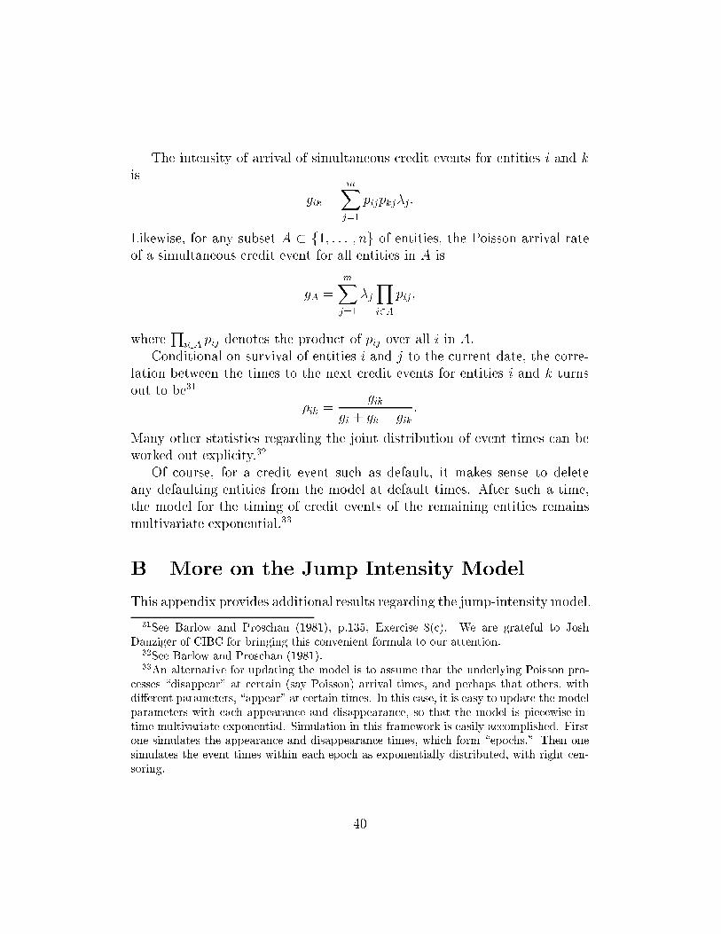
The intensity of arrival of simultaneous credit events for entities i and kis

gik =mXj=1

pijpkj�j:

Likewise, for any subset A � f1; : : : ; ng of entities, the Poisson arrival rateof a simultaneous credit event for all entities in A is

gA =mXj=1

�jYi2A

pij;

whereQ

i2A pij denotes the product of pij over all i in A.Conditional on survival of entities i and j to the current date, the corre-

lation between the times to the next credit events for entities i and k turnsout to be31

�ik =gik

gi + gk � gik:

Many other statistics regarding the joint distribution of event times can beworked out explicity.32

Of course, for a credit event such as default, it makes sense to deleteany defaulting entities from the model at default times. After such a time,the model for the timing of credit events of the remaining entities remainsmultivariate exponential.33

B More on the Jump Intensity Model

This appendix provides additional results regarding the jump-intensity model.

31See Barlow and Proschan (1981), p.135, Exercise 8(c). We are grateful to JoshDanziger of CIBC for bringing this convenient formula to our attention.

32See Barlow and Proschan (1981).33An alternative for updating the model is to assume that the underlying Poisson pro-

cesses \disappear" at certain (say Poisson) arrival times, and perhaps that others, withdi�erent parameters, \appear" at certain times. In this case, it is easy to update the modelparameters with each appearance and disappearance, so that the model is piecewise-in-time multivariate exponential. Simulation in this framework is easily accomplished. Firstone simulates the appearance and disappearance times, which form \epochs." Then onesimulates the event times within each epoch as exponentially distributed, with right cen-soring.

40

Year

SumofDefaultIntensity�=Pi�i

2

4

6

8

10

12

0 020406080100

120

HighCorrelation

MediumCorrelation

LowCorrelation

Figure10:Samplepathsoftotaldefaultintensity,summedover1,000�rms,fordi�erentcorrelations.

41

C More on the Log-Normal Intensity Model

Additional results for the log-normal intensity model are provided in thisappendix.

280

300

320

340

360

380

400

420

440

Year

95%DefaultLoss($)

1 2 3 4 5 6 7 8 9 10

� = 0:05� = 0:25� = 0:50� = 0:75� = 0:95

Figure 11: 95% Default Loss for the �rst quarter of each year. 20,000 simu-lation runs for the base case with varying volatility of default intensity.

42

Table 1: Sample mean and standard deviation (in parenthesis) of SimulatedDecile Estimates for the 1st Quarter Default Losses, in Millions of Dollars.5,000 simulations for each set of estimates. Sample statistics calculated from10 sets of estimates.

Year Con�dence Levels50% 75% 95% 99%

0 13.26 77.45 284.99 485.50( 0.61) ( 2.60) ( 6.53) (10.83)

1 14.76 85.00 302.04 513.06( 0.57) ( 3.18) (12.48) (21.19)

2 15.05 87.65 300.96 511.89( 0.98) ( 4.96) ( 7.66) (17.65)

3 15.02 86.25 299.90 511.19( 0.54) ( 2.42) ( 8.96) (21.25)

4 15.41 89.03 303.72 512.80( 0.52) ( 2.97) (13.47) (18.66)

5 15.11 87.45 303.50 513.02( 0.89) ( 4.48) ( 7.30) (13.90)

6 15.33 88.37 306.74 521.69( 0.70) ( 2.75) ( 5.37) (21.84)

7 15.04 86.77 299.95 509.42( 0.73) ( 4.75) ( 8.32) (16.04)

8 14.57 86.03 301.01 509.09( 0.63) ( 3.08) ( 8.18) (14.79)

9 14.91 90.05 306.48 512.63( 1.04) ( 2.50) ( 8.17) (22.52)

10 14.92 88.01 303.01 514.17( 0.48) ( 3.25) ( 8.70) (19.24)

43

Table 2: Sample mean and standard deviation (in parenthesis) of SimulatedDecile Estimates for the 1st Quarter Default Invents. 5,000 simulations foreach set of estimates. Sample statistics calculated from 10 sets of estimates.

Year Con�dence Levels50% 75% 95% 99%

0 1.00 2.00 3.00 4.00( 0.00) ( 0.00) ( 0.00) ( 0.00)

1 1.00 2.00 3.00 4.80( 0.00) ( 0.00) ( 0.00) ( 0.42)

2 1.00 2.00 3.10 5.00( 0.00) ( 0.00) ( 0.32) ( 0.00)

3 1.00 2.00 3.40 5.00( 0.00) ( 0.00) ( 0.52) ( 0.00)

4 1.00 2.00 3.50 5.00( 0.00) ( 0.00) ( 0.53) ( 0.00)

5 1.00 2.00 3.10 5.00( 0.00) ( 0.00) ( 0.32) ( 0.00)

6 1.00 2.00 3.00 5.00( 0.00) ( 0.00) ( 0.00) ( 0.00)

7 1.00 2.00 3.00 5.00( 0.00) ( 0.00) ( 0.00) ( 0.00)

8 1.00 2.00 3.10 5.00( 0.00) ( 0.00) ( 0.32) ( 0.00)

9 1.00 2.00 3.00 5.00( 0.00) ( 0.00) ( 0.00) ( 0.00)

10 1.00 2.00 3.00 5.00( 0.00) ( 0.00) ( 0.00) ( 0.00)

44

Table 3: Simulated Decile Estimates for the 1st Quarter Default Losses, inMillions of Dollars. 10,000 simulations runs.

Year Con�dence Levels50% 75% 95% 99%

D = 1:0 year0 13.26 80.56 281.64 483.942 15.39 84.88 303.60 498.334 14.61 88.26 305.90 500.676 15.95 91.86 312.63 529.858 14.81 85.19 303.39 504.7310 14.89 88.65 298.07 523.53

D = 0:5 year0 14.01 80.99 288.12 485.952 15.42 89.15 304.10 499.604 14.91 87.72 294.60 512.096 14.88 88.76 304.69 483.568 13.65 84.31 311.54 526.4410 14.32 85.58 302.32 521.78

D = 0:25 year0 13.18 79.61 288.65 517.702 15.38 90.34 304.36 517.584 14.66 85.50 309.05 522.206 15.22 87.00 300.71 504.998 15.43 91.28 314.25 529.7410 15.26 90.37 302.40 513.56

45

n

P(1st-QuarterDefaults�n)

0

0.1

0.2

0.3

0.4

0.5

2 4 6 8 10 12 14 16 18 20

� = 0:95� = 0:50� = 0

Figure 12: Probability of n or more defaults in the �rst-quarter of year10. (1,000 entities, intensity exponential Ornstein-Uhlenbeck, parameters� = ln(0:0017), � = 1, � = 0:5, pair-wise intensity shock correlation �).

46

Time Interval m (days)

Probabilityofanm-dayperiodwith4ormoredefaults

00

0.05

0.1

0.15

0.2

0.25

0.3

0.35

10 20 30 40 50 60 70 80 90 100

� = 0:95� = 0:50� = 0

Figure 13: Probability of an m-day period within 10 years having 4 or moredefaults (1,000 entities, intensity exponential Ornstein-Uhlenbeck, parame-ters � = ln(0:0017), � = 1, � = 0:5, pair-wise intensity shock correlation�).

47