silicon vibrating wires at low temperatures
TRANSCRIPT

HAL Id: hal-00920139https://hal.archives-ouvertes.fr/hal-00920139
Submitted on 17 Dec 2013
HAL is a multi-disciplinary open accessarchive for the deposit and dissemination of sci-entific research documents, whether they are pub-lished or not. The documents may come fromteaching and research institutions in France orabroad, or from public or private research centers.
L’archive ouverte pluridisciplinaire HAL, estdestinée au dépôt et à la diffusion de documentsscientifiques de niveau recherche, publiés ou non,émanant des établissements d’enseignement et derecherche français ou étrangers, des laboratoirespublics ou privés.
Silicon Vibrating Wires at Low TemperaturesEddy Collin, Laure Filleau, Thierry Fournier, Yuriy M. Bunkov, Henri Godfrin
To cite this version:Eddy Collin, Laure Filleau, Thierry Fournier, Yuriy M. Bunkov, Henri Godfrin. Silicon VibratingWires at Low Temperatures. Journal of Low Temperature Physics, Springer Verlag (Germany), 2008,150 (5/6), pp.739. 10.1007/s10909-009-9989-5. hal-00920139

Journal of Low Temperature Physics manuscript No.(will be inserted by the editor)
Eddy Collin∗ · Laure Filleau · ThierryFournier · Yuriy M. Bunkov · Henri Godfrin
Silicon Vibrating Wires at Low Temperatures
10.12.2007
Keywords Micromechanics, dissipation process, viscosity
Abstract Nowadays microfabrication techniques originating from micro-electro-nics enable to create mechanical objects of micron-size. The field of Micro-Electro-Mechanical devices (MEMs) is continuously expanding, with an amazingly broadrange of applications at room temperature.Vibrating objects (torsional oscillators, vibrating wires) widely used at low tem-peratures to study quantum fluids, can be replaced advantageously by SiliconMEMs. In this letter we report on the study of Silicon vibrating wire devices.A goal-post structure covered with a metal layer is driven at resonance by theLaplace force acting on a current in a magnetic field, while the induced voltagearising from the cut magnetic flux allows to detect the motion. The characteristicsof the resonance have been studied from 10 mK to 30 K, in vacuum andin 4Hegas. In this article, we focus on the results obtained above 1.5 K,in vacuum andgas, and introduce some features observed at lower temperatures.The resonant properties can be quantitatively understood by means of simple mod-els, from the linear regime to a highly non-linear response at strong drives. Wedemonstrate that the non-linearity is mostly due to the geometryof the vibrators.We also show that in our device the friction mechanisms originate in the metalliclayers, and can be fully characterized. The interaction with4He gas is fit to theorywithout adjustable parameters.
PACS numbers: 62.20.Dc, 62.40.+i, 81.40.Jj, 47.45.-n, 47.45.Ab
Institut NEEL/CNRS-UJF-INPG - 25, rue des Martyrs - Bt. E - BP16638042 Grenoble cedex 9 FranceE-mail: [email protected]

2
1 INTRODUCTION
Vibrating wires are standard probes for3He and4He liquids in their normal and su-perfluid states1,2,3. With the advent of microfabrication, micro-electro-mechanical(MEM) structures can be made and optimized4 in order to replace and transcendthis common technique5.Actually, Silicon vibrating wires are an essential feature of theULTIMA project,in which the unique properties of superfluid3He are used to make ultra-sensitivebolometers for cosmic particle detection6.Several studies on Silicon torsional oscillators at low temperatures have beenpublished7,8. In the most general context, many applications of low temperatureprobes and actuators based on torsion or flexion of Silicon structures can be en-visaged. The understanding of the mechanical properties of these devices at lowtemperatures is thus a pre-requisite.
In this paper we present our results on micron-size goal-post shaped Siliconstructures. After a brief introduction of the devices, we describeour experimentalsetup and the signatures observed in the measurements. A third theoretical partdevelops the calculations necessary for the quantitative data analysis of the fourthpart. The latter part is a brief introduction to irregularities due to very strong drives,and effects observed at the lowest temperatures. The conclusionsummarizes ourunderstanding of these devices, and introduces some future work.
1.1 The structure
The mechanical structure we consider is shown on Fig. 1. The fabrication methodhas already been reported9, but we shall quickly recall it. The sample is made from(low Boron-doped) monocrystalline<001> Silicon wafers (typically resistivityρ ≈ 25 mΩ .cm at 300K) protected by Si3N4. We start by chemically etching(KOH) a window on the back of the sample, leaving only a thin membrane. On thefront side, a metallic layer is deposited either by Joule evaporation or by means ofa magnetron. A masking layer having the desired goal-post shapeis then patterned,and protects an area of the sample from the last RIE step (Reactive IonEtching).With an Aluminum metallic layer, we use the metal itself as a mask for the Silicon.Otherwise, resist is used and removed by anO2 plasma. In the last etching step,the membrane is etched away releasing the vibrating structure. A SEM (ScanningElectron Microscope) picture of a sample is presented in Fig. 1, bottom.
The simplified theoretical structure we consider consists of two (identical) rec-tangular cantilever beams (called thereafter ”feet”) of lengthh and widthe′ (Fig.1, top). They are linked by a ”paddle” of lengthl and widtha. The average Siliconthickness ise, while the feet have an overall thickness gradientα = de
dz =Cst (dueto the chemical etching method).On top of the structure a metallic layer of thicknesseM ensures the drive and de-tection. The Laplace force
∫
Idl y∧Bz = IlB x acting on the paddle generates thedistortion in thex direction, and the motion induces a voltageV = dφcut/dt =Bl dXm/dtz.zm (Lenz’s law).dXm/dt is the speed of the extremity (zm is the di-

3
B
l
a
e’
h
e
α
eMI
x
y z
V
<110><110>
<001>
Fig. 1 (Color online). Top: schematic of the samples studied. The driving method is representedwith B andI , the detection withV. The darker color is Silicon while the lighter color on top ismetal. The geometrical parameters are presented, togetherwith the axis and their correspondingcrystallographic directions. Bottom: actual SEM picture of one sample (Eb2), with contact pads.The sample thickness is about 10µm.

4
Fig. 2 (Color online). Left: Copper support receiving the sample-holders with connecting stripes(mounted on the top-hat of the cell). On one side a thermometer while on the other a heater aremounted. Right : A sample (E6) clipped in a sample-holder (beryllium-copper springs).
rection along the distorted feet, at their end point). The effectsof the metal on themechanical properties of the structure are discussed in secion 4.2.
2 EXPERIMENT
The results reported in this article have been obtained in a4He pumped cryostat,down to 1.5K. The Silicon samples were mounted on a thick (1mm) copper platein a pumped cell (Fig. 2). On one side of the copper plate, a calibrated Allen-Bradley carbon resistor has been affixed, while on the other sidewe mounted a100Ω heater. The drive/detection setup is based on the standard vibrating wirescheme11. A twisted pair of wires allows to drive the sample with a currentI ,while another twisted pair allows us to detect the induced voltageV. A coppercoil (diameter 35mm, length 61mm) generating the external fieldB (27.58mT/Aat its center) surrounds the cell. The inhomogeneity over a couple of mm in thecenter has been calculated to be smaller than 1.5%.The signalV is brought to a (high impedance) room temperature differential pream-plifier, and fed to a lock-in detector. A DC current source provides the currentfor the coil, while an arbitrary waveform generator applying a voltage onto a100kΩ /10kΩ /1kΩ resistor (in series with the low impedance Silicon vibratingwire) generates the currentI . A commercial low frequency telecoms 1 : 1 trans-former has been used to decouple the drive from the detection. The setup has beencarefully calibrated in order to provide an absolute error onB, I andV of the order∼ 1% each. However, alignment and centering of the Silicon sample with respectto the coil are certainly imperfect, and could be the source of additional errors.The resolution onV depends obviously on the signal strength, which varied from0.1mV down to a fraction ofµV.A diffusion pump produces (at the high temperature end of the pumping line) avacuum of the order of 5.10−6Torr. We verified that continuously pumping on thecell, or closing the room temperature valve to the cell after a night’s pumping anda cool down to 4.2K gave the same experimental results. We thus call this lowpressure limit ourvacuum limit. Measurements in4He gas at 4.2K are presented

5
Fig. 3 SEM close-up of the left corner of sample E6 with its first Aluminum deposition (on top).Etching structures are visible on the metallic layer, whichslightly overruns the Silicon. The poorstraightness of the Silicon shape is due to the rather poor quality of the optical lithography.
in section 4.3.The temperature was measured and regulated with a resistance bridge. Only thecopper plate is regulated, the stainless steel cell is kept immersed in liquid He-lium. For each change of temperature, a settling time of at least half an hour wasallowed. The calibration of the thermometer is believed to be accurate to∼ 2%approximately.
In the following we present the measured resonance lines, and inferexper-imentally the coefficients and parameters describing the vibrating structure andits constitutive materials. Various samples have been tested, and on one of them(E6) we added metaltwo times, on both sides, in order to properly extract its con-tribution. We used the Joule evaporation technique. The metal(99.99%-Al) wasdeposited at a rate comprised between 10A/s and 40A/s, in a vacuum of about10−5Torr. The sample wasnot cleaned between evaporations. The first metallicdeposition served also as a protection for the Silicon structure in the last etchingstep (RIE) of the fabrication process. A close-up SEM image is shown in Fig. 3.The theoretical expressions of part 3 are used in the quantitative data analysiswhich is postponed to part 4. These theoretical fits and the careful measurementsrealized in a very broad range of parameters at low temperatures, constitute thecore of this article, demonstrating our understanding of these devices.
2.1 Resonance properties
In Fig. 4, we present three typical resonance lines obtained for very different drivesin vacuum at 4.2K. We define, written in complex terms,V(ω) = V ′+ iV ′′ for the

6
-1 10-6
-5 10-7
0
5 10-7
1 10-6
1.5 10-6
2 10-6
4194.56 4194.64 4194.72
V',
V''
(Vrm
s)
-5 10-6
-2.5 10-6
0
2.5 10-6
5 10-6
7.5 10-6
1 10-5
4194.56 4194.68 4194.80-1 10-4
-5 10-5
0
5 10-5
1 10-4
1.5 10-4
2 10-4
4192 4204 4216
Frequency (Hz)
Fig. 4 (Color online). Three resonance lines measured in vacuum at4.2K with different drives(sample E6 with first metal deposition). The magnetic field was 11mT. The dark (or blue) crossesare the in-phase signalsV ′, while the light (pink) crosses are the out-of-phaseV ′′ voltages.From left to right: linear signal, force 11pNrms and displacement 3.3µmrms; non-linear signal,force 69pNrms and displacement 18µmrms (the arrows indicate the sweep direction, showinghysteresis); very non-linear signal, force 4.6nNrms and displacement 0.33mmrms (up sweep).The black lines are fits (see text).
detected voltageV in Fourier space, withω = 2π f the angular frequency (andi =
√−1). In part 3, the (harmonic) displacementXm(t) of the end of the structure
is described with the resonance componentsXPm andXQm (in-phase and out-of-phase displacements respectively).V ′ = lBω XQm is the in-phase signal detected,andV ′′ = lBω XPm the out-of-phase signal.V ′ is a peaked function and from itsmaximumV ′
max we calculate the maximum displacementXmax reached by the topof the structure. Most of the values quoted in this article arerms (root-mean-square), which derive from the peak amplitude withxrms = x0/
√2. The signal is
measured while sweeping the frequency (usually upwards otherwisethe directionis stipulated). For each point, a settling time of the order of 1/(π ∆ f ) has beentaken to reach the steady-state limit (∆ f being the full width at half height of theV ′ component).The resonance lines are studied for various temperatures and driving forces. Atsmall drives, the response of the mechanical system is always linear, while forhigher drives we are able to reach a highly non-linear regime. Thisis presented inFig. 4. From left to right, we show a resonance obtained at the end of the linearregime, then a non-linear measurement displaying the usual features of non-linearresonances, and at last a very non-linear line obtained for displacementsXmax ofthe order of 0.33mmrms. This last measurement is remarkable, in the sense thatthe peak-to-peak displacement is of the order of 0.9mm for a structure of lengthh = 1.35mm. The distortion isextreme, the angle swept by the structure being ofthe order of 40.
The black lines are fits, withXPm andXQm obtained from Eq. (24) and Eq.(25) respectively (part 3). For small displacements (small drives),they reduce totheLorentzexpressions, Eq. (16) and Eq. (17).In this linear regime (left graph Fig. 4), some useful and well-known propertiescan be given forV(ω). TheV ′ component is maximum atf = fres, with V ′′ = 0

7
10-6
10-5
10-4
10-12 10-11 10-10
Dis
plac
emen
t (m
rms)
Force (Nrms
)
Fig. 5 (Color online). DisplacementXmax versus forceFac curve for sample E6 (first metaldeposition) in vacuum at 4.2K (logarithmic scale). The thick line is a fit, which associated to themeasurement of the full width∆ f enables to extract the vibrating mass of the object (Tab. 2).Atstrong drives, non-linear effects are already visible (discrepancy between dashed and full lines)and will be discussed in the following paragraphs. Error bars are of the order of 5% altogehter.
(resonance point). The heightV ′max is proportional to the forceFac applied, and in-
versely proportional to the full-width-at-half-height∆ f of theV ′ line. In fact, thisproperty can be used to ”weigh” experimentally the wire, extracting the vibrating(or normal) massmv0 (see Fig. 5). For sample E6 and the first metal deposition,we obtained 1.35µg (Tab. 2). The quality factor defined asQ = fres/∆ f is of theorder of 0.3106 which is a remarkable figure.When the driving force becomes too strong, the resonance enters thenon-linear
regime. One has then to solve numerically (see fits of Fig. 4) Eq. (24) and Eq.(25). At first, the resonance line is pulled toward higher frequencies (for a positivenon-linear coefficientb0 introduced in part 3; it is obviously inverted for the otherpolarity). At some critical drive, the equations to solve get multi-valued: two stablesolutions appear, one stable while sweeping the frequency up,and the other whilesweeping down (see middle graph Fig. 4). Hysteresis appears, and close to themaximal amplitude point on theV ′ component, the device switches from motionto stillness (so-called bifurcation point). The in-phase signalV ′ looks practicallytriangular, and the out-of-phaseV ′′ practically circular. The last remains almoston the positive side, even above the bifurcation point. At very strong drives, thehysteresis is so large that practically no resonance can be detected on the downsweeps (right graph Fig. 4).However, some simple criteria still do apply. If one sweeps the frequency upwards(in fact, in the direction corresponding to the polarity of the non-linear coefficientb0), the signalV ′ is still maximum at the so-called resonance frequencyfres de-fined in section 3.5, andV ′′ is still zero. The maximum heightV ′
max of the peakV ′
is still proportional toFac and inversely proportional to∆ f . But now, fres and∆ fare functions of the displacement Xmax (involving the coefficientsb0 andb1 pre-sented in part 3), which in turn has to be evaluated at resonance. As a consequence,

8
10-5
10-4
10-3
10-2
10-1
100
101
102
10-6 10-5 10-4 10-3
Fre
quen
cy s
hift
(Hz)
Displacement (mrms
)
4194.665 Hz
Fig. 6 (Color online). Non-linear frequency shift as a function ofthe displacementXmax (notethe logarithmic scale), measured in vacuum at 4.2K (sample E6, first metal deposition). Thelinear resonance frequency given on the picture has been subtracted. The line is the quadraticdependence expected from theory, fit on the data.
∆ f cannot be measured anymore as the half-height width of theV ′ component.Moreover, the theoretical model of section 3.5 predicts a non-linear detected sig-nal V, through theb3 parameter, which implies a non-linear dependence of themaximum measured heightV ′
max with respect toXmax. The key result of the the-oretical description is thatif the non-linearities originate from the geometry ofthe distortion, all non-linear parameters (fres, ∆ f , V ′
max) have to display a(Xmax)2
dependency, from which the correspondingbi factor can be experimentally deter-mined.
The non-linear behavior of the resonance frequency is presented on Fig. 6.Indeed, the dependence of the frequency shift on the displacement is quadratic,over the entire explored range,includingvarious magnetic fields and various (non-linear) dampings. On the other hand, Fig. 7 presents the inversenormalized height1/(V ′
max/Fac). This parameter depends directly onXmax through theb3 factor, butis also simply proportional to the linewidth∆ f (damping term). The striking re-sult of Fig. 7 is that this parameter appears clearly to be alinear functionof thedisplacement, in complete disagreement with the (simple geometrical) theory pre-dicting a quadratic dependence.The apparent paradox is lifted as soon as we realize that the increase of the
dissipation (increase in∆ f ) is due to the materials’ response rather than sim-ple (geometrical) non-linearities. In order to unambiguously prove that the lineardependence toXmax of the inverse normalized height originates in∆ f , one canconsider thepower balanceat resonance. Indeed, exactly at resonance (wheredrive Fac and speed ˙x are in-phase, sinceV ′′ = 0), the (mechanical) potential en-ergy 1/2kv0x2 is simply transferred to kinetic energy 1/2mv0 x2 and vice-versa(throughkv0xx = −mv0 xx), while the drive balances the dissipated energy. Thismeans that the (electrical) injected powerFac x = V I is exactly equal to∆ω mv0 x2

9
0.5
1
1.5
2
2.5
3
3.5
4
4.5
0 1 10-4 2 10-4 3 10-4 4 10-4
Nor
mal
ized
inve
rse
heig
ht (
a.u.
)
Displacement (mrms
)
Fig. 7 (Color online). Inverse normalized height 1/(V ′max/Fac) measured in vacuum at 4.2K
for sample E6 (first metal deposition), as a function of displacementXmax. The line is a lineardependence, fit on the data, which isnot expectedfrom the geometrical theory of non-linearities.
10-14
10-13
10-12
10-11
10-10
10-9
10-8
10-7
10-14 10-13 10-12 10-11 10-10 10-9 10-8 10-7
Dis
sipa
ted
pow
er (
W)
Injected power (W)
Fig. 8 (Color online). Power balance obtained from Fig. 7, assuming that the height non-linearity arises solely from the damping term∆ f . The line represents equality of powers injectedand dissipated (see text). Symbols are as large as±5% error bars.
(the dissipated power). The key point is that the calculated injected power dependslinearly on the detected voltage and is independent of the measured width, whilethe calculated dissipated power dependsquadratically on the detected voltage andis proportional to the measured width. Assuming that the non-linear height (Fig.7) is indeed a direct image of the width, we plot on Fig. 8 the powers averagedover one oscillation period. The calculated points are exactly on the equality line(full black line) which proves that the assumption is correct: thelinewidth∆ f is alinear function of displacement, or speed.

10
We thus have to conclude that quadratic (geometrical) non-linear correctionson the resonance’s height and width are negligible, a point explained in part 4.Furthermore, as in any low temperature experiment, it is legitimate to considerthermal gradients and question the temperature’s homogeneity.Indeed, the line-width’s linear dependence to the displacement could be obtained with a thermalmodel. However, a quantitative analysis described in the following section allowsus to rule out this possibility for our devices.
2.2 Absence of thermal gradients
Two sources of heating are present, the mechanical power dissipated∆ω mv0 x2
already introduced, and the Joule heating due to the resistivity of the metal layerRel I2. We write I = I0 cos(ωt) and x = x0 cos(ωt + ϕ). For the sake of simplic-ity, we consider that this power is created at the end of the structure, and leakstoward the thermal bath (the copper support) through the metal layer. As shall bediscussed in part 4, since the dissipation process takes placein the metal itself, webasically neglect completely the Silicon(1).Disregarding non-linear effects, we write for the heat equation:
ρMCM∂T∂ t
−κM∂ 2T∂x2 = 0
with ρM, CM and κM the density, specific heat and thermal conductivity of themetal, respectively. The boundary conditions are:
T(x = 0, t) = T0,
κM e′eM∂T∂x
(x = h, t) =12
Q0 +12
∆Q cos(2ωt +φ)
where the first equation stands for the bath temperature, and the last for the heatflow (the factor 1
2 reminding that there are two feet in the structure). With ournotations:
Q0 =12
∆ω mv0 x20
(
1+Relmv0 ∆ω(l B)2
)
,
∆Q =12
∆ω mv0 x20
√
1+Relmv0 ∆ω(l B)2
(
2cos(2ϕ)+Relmv0 ∆ω(l B)2
)
while tanφ = sin(2ϕ)/[Relmv0 ∆ω(l B)2 +cos(2ϕ)]. We defineCth = ρMCM(he′eM) the
heat capacity andRth = κ−1M h/(e′eM) the thermal resistance of one foot of the
structure.τ = RthCth is the thermalization time constant. The temperature at theend of one foot is:
T(x = h, t) = T0 +12
Q0hκM e′eM
+12
∆QhκM e′eM
1√ωτ
cos(2ωt +φ −π/4), (1)
1 A more complete model would only give a better thermal link; distributing the power dissi-pated along the feet of the structure reduces the temperature gradients too.

11
or
T(x = h, t) = T0 +12
Q0hκM e′eM
+12
∆QhκM e′eM
1√2
cos(2ωt +φ +π/4) (2)
where the first equation stands for a poor heat conduction (ωτ ≫ 1), and the lastfor a good heat conduction (ωτ ≪ 1).
We take for the measured damping parameter∆ω = 2π∆ f a linear func-tion of temperatureT, as obtained experimentally in part 4, producing∆ω(T) =∆ω(T0)+ β ∆T. ∆T is the temperature increase of the region where friction oc-curs; in our simplified model the end of one foot.β is an experimental parametercharacterizing the intrinsic damping mechanism, which has to be measured.We take for the metal’s thermal conductivityκM = κ0T and for the electricalresistivity a constant valueρel. Both are linked through the Wiedemann-Franzlaw κM ρel = LT with L the Lorenz number (see Ref.28 for a discussion on Alu-minum). The specific heat of the metal layer29 writesCM = γ T. We express the(total) electric resistance asRel = ρel [(2h)/(eM e′)+ l/(eM a)].Two cases have to be distinguished:
– Poor thermal link: the temperature’s oscillatory part in Eq. (1) averages out,and only a (large) static temperature increase is present at the end of the struc-ture. It writes at the lowest order:
∆T = xrms
√
12
mv0 ∆ω(T0)
(
1+Rel mv0 ∆ω(T0)
(l B)2
)
Rth(T0)T0−12
T0
with xrms = x0/√
2. The linear dependence to ˙xrms generates in turn a lineardependence to ˙xrms in ∆ω . Although it reproduces theanalytic dependencemeasured (Fig. 7), aquantitativeanalysis fails(2). Our devices arenever inthis limit.
– Good thermal link: the temperature at the end of the structure oscillates with anamplitude almost as large as the average thermal gradient. However, whetherthe dissipation process will follow this oscillation or not depends on its intrin-sic characteristic timescale, which is unknown. The (small) static temperaturegradient writes at first order:
∆T = x2rms
12
mv0 ∆ω(T0)
(
1+Rel mv0 ∆ω(T0)
(l B)2
)
Rth(T0)
which displays a quadratic dependence to ˙xrms. Using values from the literaturefor Aluminum28,29,48demonstrates that∆T ≪ T0, and the thermal contact isalways excellent(3): the temperature of the vibrating structure is uniform to anexcellent approximation, and always equal to the measured temperatureT0.
2 A fit of the data using this expression generates for the Aluminum metallic layer such a badthermal conductivity that the RRR (so-called Residual Resistivity Ratio) would besmallerthan1, which is unphysical.
3 The discussion basically holds for any non-superconducting metal with a reasonable RRR(Residual Resistivity Ratio), with any (reasonable) thickness, and not too low temperatures.

12
We conclude that the linear dependence of the resonance curve’s inverse heightas a function of the displacement, seen in Fig. 7, is genuine and originates froman intrinsic linear dependence of∆ f to Xmax. This effect is clearly due to thematerials, and shall be described by some specific model: we introduce non-lineardamping coefficientsΛ ′
1 and Λ ′2 arising from theshear thickening fluid model
presented in section 3.4.
2.3 Fits of the resonance curves
The black lines in Fig 4 are fits obtained by solving numericallyEq. (24) and Eq.(25). To obtain these fits,only one set of parametersis used over the entire para-meter space (drive, temperature, fields, and even pressure). These parameters arein agreement with direct measurements like the determination ofthe mass (Fig.5), or the (geometrical) non-linearb0 parameter and the (friction) non-linearΛ ′
1,2parameters (Figs. 6 and 7 respectively). The values extracted from these analysesshall be discussed in part 4.The data analysis producing the fit considers a perfectly stable phase reference forthe setup (lock-in plus generator). Only a base-line is subtracted,with a resistive(onV ′) and a reactive (onV ′′) component. Both components are taken to be linearwith respect to the frequency sweep, that is either the background is a linear func-tion of f , or its magnitude changes weakly with time. For narrow sweeps or smalltemperature drifts, this procedure is perfectly justified. The fits areexcellent. Thesmall discrepancies in Fig. 4 are mostly due to the finite-time needed to sweep theline (especially at the bifurcation point) or drifts in the circuitparameters. Limita-tions of the model are discussed in part 5.
3 THEORETICAL DESCRIPTIONS
In this section we present the theoretical approaches used in order to quantitativelydescribe our results. The aim is to useexclusivelyanalytical expressions, withoutany numerical simulations. The simplifications we apply are thoroughly discussed.We shall start by introducing the required formulas specialized toour structure,and pursue with a refined application of the Rayleigh method to the non-linearresonance case. A discussion of the friction signature is presented.
3.1 Simple static distortion
We first consider the simplest case of a static linear distortion, for a straight (α = 0)and ideally thin structure. We take into account the presence of(homogeneous)stress in the Silicon, along the feet and the paddle, which can arise from the metaldeposition(4). It is modeled with two static forcesS, one alongy (paddle) and onealongz (feet), which sign depend on the stress type (tension or compression).
4 In one very thin sample (less than 5µm) covered with NbTi, the authors even noticed underthe SEM a strong static distortion of the paddle of the structure. The influence of the metal layeris discussed in detail in the oncoming experimental sections.

13
The aim is to demonstrate that thelowest modeof the structure is simply the back-and forth oscillation of the feet clamped together by the paddle. This mode is theone we presented in part 2, and study quantitatively in part 4.
3.1.1 Paddle distortion
In order to calculate the shapeX(y) of the paddle distortion, we assume that theclamping of the paddle with respect to the feet is ideal (X = 0, dX/dy = 0 aty = 0, l ). The force is taken to be homogeneously distributed along the paddle(dF/dl = IB =Cst). The results are12:
X(y) =+l
(
Fl2
EyIy
)
1u4
[
+u/2tanh(u/2)
(
coshu(1/2−y/l)cosh(u/2)
−1
)
+u2
2y(l −y)
l2
]
,
or
X(y) = −l
(
Fl2
EyIy
)
1u4
[ −u/2tan(u/2)
(
cosu(1/2−y/l)cos(u/2)
−1
)
+u2
2y(l −y)
l2
]
whereu =√
|S|l2EyIy
and the first expression stands for tension (S> 0 with our nota-tions) and the second for compression (S< 0). F is the total force (IlB), Ey standsfor the Young’s modulus along they axis, andIy the corresponding moment ofinertia for flexion. With our notations, we getIy = 1
12ae3.
Assuming that the stressS is small with respect toEyIy/l2 (u≪ 1), we write:
X(y) = Xm
[
(
+16(y/l)2−32(y/l)3 +16(y/l)4)
±u2(
+2(y/l)2−12(y/l)3 +26(y/l)4−24(y/l)5 +8(y/l)6
15
)
]
(3)
whereXm = l(
Fl2EyIy
)[
1384− ±u2
15360
]
is the maximal deflection aty = l/2. The elon-
gation of the paddle due to the forceF has a second order signature on the axialstressS, which is neglected here. The± stands for the sign ofS; the first orderterm in stress is a quadraticu2.The bending momentMz at each end of the paddle is then:
|Mz| = |F | l(
112
− ±u2
720
)
. (4)
The force exerted at the ends has an axial component±Salongy (up to a secondorder inF), and a shear component of magnitude|F |/2 alongx.The stress tensorσ in the Silicon has only three nonzero components:
σyy(x,y) =Sea
+12Fea
le
[
(x/e)− 12
]
[
(
112
− (y/l)2
+(y/l)2
2
)
± u2(
− 1720
+(y/l)2
24− (y/l)3
12+
(y/l)4
24
)
]
, (5)

14
σyx,xy(x,y) =3Fea
[
(
−(x/e)+(x/e)2)(
1−2(y/l))
± u2(x/e)(y/l)(
1− (x/e))
(
1−3(y/l)+2(y/l)2
6
)
]
(6)
where the double subscriptyx,xy recalls the tensor symmetry (x running from 0 toe).
If we assume that there is no slippage at the metal/Silicon interface, one caneasily take into account the finite Young’s modulus of the metal layer. The actualstructure is then equivalent to an all-Silicon ”T-shaped” beam, where the width ˜aof the top part (of thicknesseM) is:
a = aEM
Ey
whereEM is the Young’s modulus of the metal layer. By doing so, one hastoreplace in the above equations the moment of inertia by:
Iy −→112
a2e4 + a2e4M +4aeaeM(e2 +e2
M + 32eeM)
ae+ aeM. (7)
In our case (using mostly Aluminum), typicallyEM/Ey ≈ 0.4 andeM/e< 0.15,thus the correction is small, but measurable.
3.1.2 Feet distortion
We proceed in the same way for the feet. The shapeX(z) of each foot’s distortion iscalculated by assuming a perfect clamping of the foot at its basis (X = 0,dX/dz=0 at z= 0). The forceF is taken to be applied at the end of the foot, where thepaddle is anchored. The results are12:
X(z) =
+h(
Fh2
EzIz
) 1u3(u−1+coshu)
[
+u(1−u)(1−z/h)
+ cosh(u)(uz/h− tanh(u))+(1−u)(sinh(uz/h)−ucosh(uz/h))
+ sinhu(1−z/h)
]
,
or
X(z) =
−h(
Fh2
EzIz
) 1u3(u−1+cosu)
[
+u(1−u)(1−z/h)
+ cos(u)(uz/h− tan(u))+(1−u)(sin(uz/h)−ucos(uz/h))
+ sinu(1−z/h)
]

15
whereu=√
|S|h2
EzIzand the first expression stands for tension (S> 0) and the second
for compression (S< 0). From the previous section, the notations are straightfor-ward, and we haveIz = 1
12e′e3.
Assuming that the stressS is small with respect toEzIz/h2 (u ≪ 1), we canagain develop the expressions and write:
X(z) = Xm
[
(
32(z/h)2− 1
2(z/h)3
)
± u
(
(z/h)2− (z/h)3
4
)
]
(8)
whereXm = h(
Fh2
EzIz
)
[
13 − ±u
6
]
is the maximal deflection atz= h. The± stands
again for the sign ofS. Note thelinear dependence tou. The bending momentMyat the clamping end of the foot is then:
My = Fh
(
1− ±u3
)
(9)
while the shear force exerted (alongx) at the same end is of course−F , and theaxial force (alongz) is by definition−S.The stress tensorσ in the Silicon has only three nonzero components:
σzz(x,z) =S
ee′+
12Fee′
he
[
(x/e)− 12
][
1− (z/h)− ±u3
]
, (10)
σzx,xz(x,z) =6Fee′[
−(x/e)+(x/e)2] (11)
where the double subscriptzx,xz recalls the tensor symmetry (andx runs from 0to e).
Assuming that there is no slippage at the metal/Silicon interface, we treat thefinite Young’s modulus of the metal layerEM as in the previous paragraph. Intro-ducinge′ = e′EM/Ez, the moment of inertia becomes:
Iz −→112
e′2e4 + e′2e4M +4e′ee′eM(e2 +e2
M + 32eeM)
e′e+ e′eM(12)
which is again a small correction to the standardIz.
3.1.3 Structure behavior
We shall see in section 3.2.2 that for the first mode of vibration of our beams (feetor paddle), the peak deflectionXmax of the maximal displacementXm(t) obtained

16
at resonance by anac force of peak valueFac, is equal(5) to the static deflectionXm obtained with a forceFdc:
Fdc = QFac
whereQ is the quality factor of the mode resonance. Besides, the static shapes Eq.(3) and (8) are fairly good approximations of the dynamical shapes.Indeed, one can calculate approximative dynamical parameters of the first paddleand feet modes from these shapes. This energetic method, calledthe Rayleighmethod13, consists in integrating the elastic energy and kinetic energy along thebeam, with the time dependence incorporated inXm → Xm(t). For instance withthe foot distortion:
12
kvXm(t)2 =12
∫ h
0
(
d2X(z, t)dz2
)2
(EzIz)dz,
12
mv
(
dXm(t)dt
)2
=12
∫ h
0
(
dX(z, t)dt
)2
(ρee′)dz
which define respectively the spring constantkv and the vibrating massmv associ-ated to each foot (for the first mode).ρ is the mass density of Silicon. The samekvcan be derived by writing the constitutive equation of the elastic force at the endof the foot:Fdc = kvXm. These equations are easily transposed to the paddle case.
In order to take into account the metallic layer, one has to changeIz accordingto the previous section, and also to replaceρe→ ρe+ρMeM in the above equations(ρM being the metal density).
We shall see that this knowledge is enough to produce a good description oftheglobalshape of the dynamically distorted structure.Consider first the paddle’s clamping hypothesis. Due to the stressS along thepaddle, each foot will tend to have a distortion along they axis (adapting Eq. (8)):
|Ym| = h
( |S|h2
EzI ′z
)[
13− ±u
6
]
whereI ′z = 112ee′3 (note the inversion betweene′ ande from Iz; theu here is the
one generated by the stressalong the foot). Depending on the sign ofS, the feeteither bend inwards or outwards.The bending moment Eq. (4) at each end of the paddle tends to twist the feet byan angle:
|θ | = |Fdc| l
(
112
− ±u2
720
)
hGzJz
whereGz is the Silicon shear modulus (alongz) andJz = 112(e
′e3 +ee′3) the cor-responding moment of inertia (u is here the one associated to the stressalong thepaddle). Obviously, the feet’s twist is always oriented toward the bending forceFdc.
5 Within the approximation identifying the static spring constant (and thekv defined in thissection) and the normal spring constantkn of the first mode, which amounts to±3% discrepan-cies maximum.

17
Using the typical geometrical dimensions of our devices (say,sample E6) andthe SiliconEz andGz values16 (160GPa and 80GPa respectively), we get for themaximum solicitation(6) we consider (S≈60 µN andFdc ≈0.4mN, part 4):
|Ym| < 1%h,
|θ | < 2.
These are negligible (even when the resonance becomes highly non-linear), andwe can safely state that the clamping hypothesis of the paddleis justified.Consider now the distortion of the paddleitself under the solicitationFdc. Themaximum deflection in the middle is (applying Eq. (3)):
Xm = l
(
Fdc l2
EyIy
)[
1384
− ±u2
15360
]
.
Using the maximum values of part 4 we get:
|Xm| < 1% l
which, again, is negligible, even at the largest distortions. We can thus state that,as far as the feet’s flexion is concerned, the paddle is always perfectly rigid.
These considerations allow toidentifysimply the two first modes of the wholestructure. One is the flexion of the feet together with the rigid paddle, and one isthe oscillation of the paddle at the end of rigid feet (which, according to the abovevalue ofXm, is very poorly excitable).
Using the Rayleigh method we can approximate these two modes.The vi-brating mass and spring constant of the feet give an angular frequency ω0 =√
2kv/(2mv +mpaddle) for their first mode (the feet are loaded by the paddlemassmpaddle). For the paddle, the same procedure gives an angular frequencyω0 =
√
kv/mv for the first clamped mode.In Tab. 1 we summarize the expressions obtained within this approximation. Com-
Property For (loaded) feet For (clamped) paddle
kv 3 EzIz/h3 10245
(
1+ ±u2
420
)
EyIy/l3
mv33140
(
1− ±8u99
)
ρee′h 128315
(
1+ ±u2
660
)
ρeal
ω0 2√
3511
√
11+70/33η
(
1+ ±4u99+210η
)√
EzIz/h3
ρee′h 6√
14(
1+ ±u2
2310
)
√
EyIy/l3
ρeal
Table 1 Rayleigh’s method parameters (see text).± denotes the stress sign, source of the termu. For the loaded feet, we introduced the reduced parameterη = (al)/(e′h) (ratio of paddle massto foot mass). The metal contribution has been omitted for clarity.
paring with section 3.2.1 the prefactors 2√
35/11 and 6√
14 give fairly good es-timates of the mode positions. However, the influence of the stress termu fails to
6 These estimates neglect non-linearities; the same conclusions are reached with the non-linear expressions of section 3.3.
18
be describedcorrectly. Thus, an accurate modeling of the linear response of thesystem requires the exact time-dependent solution given in thenext section.
3.2 Simple harmonic treatment
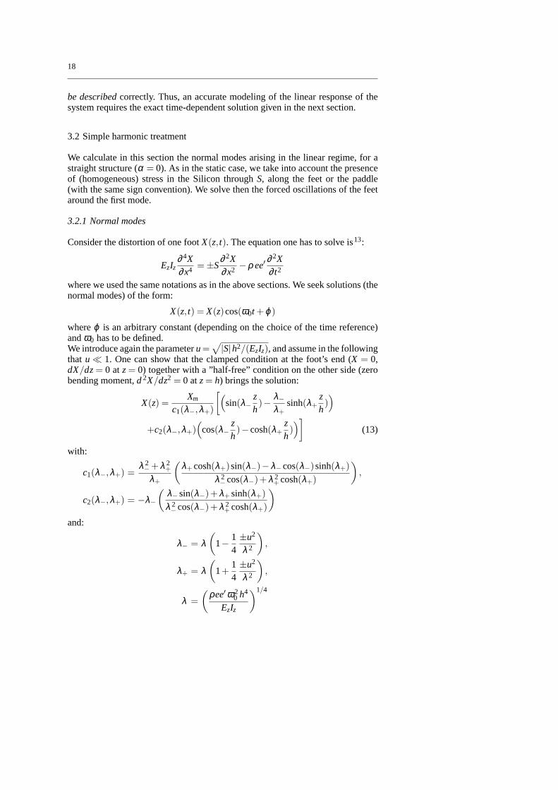
We calculate in this section the normal modes arising in the linear regime, for astraight structure (α = 0). As in the static case, we take into account the presenceof (homogeneous) stress in the Silicon throughS, along the feet or the paddle(with the same sign convention). We solve then the forced oscillations of the feetaround the first mode.
3.2.1 Normal modes
Consider the distortion of one footX(z, t). The equation one has to solve is13:
EzIz∂ 4X∂x4 = ±S
∂ 2X∂x2 −ρ ee′
∂ 2X∂ t2
where we used the same notations as in the above sections. We seek solutions (thenormal modes) of the form:
X(z, t) = X(z)cos(ω0t +ϕ)
whereϕ is an arbitrary constant (depending on the choice of the time reference)andω0 has to be defined.We introduce again the parameteru=
√
|S|h2/(EzIz), and assume in the followingthat u ≪ 1. One can show that the clamped condition at the foot’s end (X = 0,dX/dz= 0 atz= 0) together with a ”half-free” condition on the other side (zerobending moment,d2X/dz2 = 0 atz= h) brings the solution:
X(z) =Xm
c1(λ−,λ+)
[
(
sin(λ−zh)− λ−
λ+sinh(λ+
zh))
+c2(λ−,λ+)(
cos(λ−zh)−cosh(λ+
zh))
]
(13)
with:
c1(λ−,λ+) =λ 2− +λ 2
+
λ+
(
λ+ cosh(λ+)sin(λ−)−λ− cos(λ−)sinh(λ+)
λ 2− cos(λ−)+λ 2
+ cosh(λ+)
)
,
c2(λ−,λ+) = −λ−
(
λ− sin(λ−)+λ+ sinh(λ+)
λ 2− cos(λ−)+λ 2
+ cosh(λ+)
)
and:
λ− = λ(
1− 14±u2
λ 2
)
,
λ+ = λ(
1+14±u2
λ 2
)
,
λ =
(
ρee′ ω20 h4
EzIz
)1/4

19
where the± sign stands for tension (S> 0) or compression (S< 0). Note that wetake into account the finite thickness of the metal layer withthe same change ofρeandIz than in the previous section. In the above equations,λ has to be determinedby means of the last boundary condition:
EzIzd3Xdz3 (h) = −mpaddle
2ω2
0 X(h)
which states that the shear force at the endz= h is due to the inertia of the foot’sload (which is, due to symmetry, half of the paddle’s mass inertia(7) per foot). Thesolution can be written in the form:
λ = λi(η)
(
1− ±u2
2φi(η)
)
(14)
whereλi(η) is the solution without stress (u = 0) andφi(η) is the sensitivity tostress (for modei). Both depend on the ratioη = (al)/(e′h) of the paddle massto the foot mass. Indeed, the mode position is highly sensitive14 to the end loadmpaddle/2.These functions can be determined numerically for each mode; in particular forthe first onei = 0 good asymptotic expressions are:
λ0(η) =
[
(λ00)4/4+3η/2
1+η/21
1/4+η/2
]1/4
,
φ0(η) = 0.034712+0.21210η/2,
λ00 = 1.87510
with λ00 the well-known value assigned to the first mode of the ideal cantilever.The first expression fits within 0.1 % and the second within 0.5 % at worst. Thisapproach considered a bulk stress sourceS without stipulating its origin. We re-fer to the discussion of part 4 dealing with the (controversial) issue of surfacestresses15, and our related quantitative analysis.The corresponding solutions can be produced for the paddle, withclamped condi-tions on both sides (and of course no load). One finds thenλ00 = 4.7300 which isthe well-known position of the first mode of the ideally clampedbeam.With the experimental parameters of part 4, one can then easily verify that the feetmode, which is the one of interest to us, and the (weakly excitable) paddle modeare very well separated.
From the above expressions, one can interestingly notice that as the ratioηincreases, the dynamical shape becomes closer and closer to the static one weobtained in section 3.1.2; as far as theshapeof the distortion is concerned, theRayleigh method appears to be rather accurate. Indeed, comparingthese first modepositions to the ones obtained in the previous section by the Rayleigh method (Tab.1), we see that the disagreement is always smaller than 1.5% (andfalls to zero asη →+∞). However, note the differences in the incorporation of stress (throughu)in the solution.
7 A slight asymmetry between the feetonlyshifts the paddle mass-per-foot one has to considerin this calculation.

20
3.2.2 Forced oscillation
In order to compute the response of the system to a harmonic forceF(t)= Faccos(ωt)of (arbitrary) angular frequencyω , we apply the method of the virtual work13.Take for the (general) distortion of one foot the expression:
X(z, t) =+∞
∑i=0
X(i)m (t)Xi(z)
and for the virtual displacement:
δ (z, t) = ∆(t)Xj(z)
where theXl (z) functions are the (normalized) normal modes(8) of the foot and
X(i)m (t), ∆(t) time-dependent (maximal) deflections. TheX(i)
m (t) have to be defined,and the∆(t) shall disappear at the end of the calculation.Using these expressions we write the terms appearing in the powerbalance. Weget, integrating alongz, for one foot:
δW jI = −(ρee′)∆(t)
∞
∑i=0
X(i)m (t) hγi, j ,
δW jE = −(EzIz)∆(t)
∞
∑i=0
X(i)m (t) γi, j/h3
where the first is the inertia term, and the second the elastic term (dots are time-derivatives). For the end load acting on one foot we get:
δW jI ,mpaddle
= −12
mpaddle∆(t)∞
∑i=0
X(i)m (t) Xi(z= h)Xj(z= h),
δW jE,mpaddle
= +EzIz∆(t)∞
∑i=0
X(i)m (t) X′′′
i (z= h)Xj(z= h)
where the first is the inertia term (of the half-paddle), and the secondthe restoringforce. One has of course to add the work due to the external force:
δW jF = +F(t)∆(t)Xj(z= h).
In the above expressions, one has to make use of the definitionXi(z= h) = Xj(z=h) = 1. In order to keep the equations simple, we will neglect in the following thedependence to stress(9) (u=0). We introduced the quantities:
γi, j = h3∫ h
0
d4Xi
dz4 (z)Xj(z)dz= +λ 4i γi, j ,
X′′′i (z= h) =
d3Xi
dz3 (z= h) =−η/2 λ 4
i
h3
8 That is Eq. (13) from the previous section withXm = 1, andλ equal to the mode valueλl ,Eq. (14).
9 Indeed, the stored stressScouples the normal modes (see discussion of part 5). Moreover,extractingS from the measurements is a non-trivial issue (sections 3.4 and part 4).

21
together with:
γi, j =1h
∫ h
0Xi(z)Xj(z)dz
which verifies:
γi, j = γ j when i= j,
= −η/2 when i6= j.
Adding up all the terms of the power balance and using the equations above, onefinally gets, for the whole structure:
2
[
ρee′hγ j +ρeal
2
]
X( j)m (t)+2
EzIzh3 λ 4
j
[
γ j +η2
]
X( j)m (t) = F(t). (15)
We recognize the simple one-dimensional forced oscillator expression withk( j)n =
(EzIzh3 )λ 4
j
[
γ j +η2
]
(normal spring) andm( j)n = (ρee′h)
[
γ j +η2
]
(normal mass) as-sociated to each foot.A good asymptotic expression for the first modeγ j = γ0(η) is (again neglectingthe stress termu):
γ0(η) =14 + 33
140 4.418η/2
1+4.418η/2
which fits the numerical result within 0.1%.
In section 3.4 we will model friction through a dissipation term proportional
to speed, namely−2Λ1 X( j)m (t), and a reactive term proportional to acceleration,
−2Λ2 X( j)m (t). Injecting in Eq. (15) and solving for the harmonicF(t), the expres-
sion ofX( j)m (t) becomes:
X( j)m (t) = XP( j)
m cos(ωt)+XQ( j)m sin(ωt)
with
XP( j)m =
Fac
k( j)n
1− (ω/ω( j)0 )2−2δω ω/(ω( j)
0 )2
[
1− (ω/ω( j)0 )2−2δω ω/(ω( j)
0 )2]2
+[
∆ω ω/(ω( j)0 )2
]2 , (16)
XQ( j)m =
Fac
k( j)n
∆ω ω/(ω( j)0 )2
[
1− (ω/ω( j)0 )2−2δω ω/(ω( j)
0 )2]2
+[
∆ω ω/(ω( j)0 )2
]2 (17)
whereXP( j)m is the (peak) in-phase motion, andXQ( j)
m the (peak) out-of-phase
motion (with ω( j)0 =
√
k( j)n /m( j)
n the angular frequency of modej). We intro-
ducedδω = ωΛ2/m( j)n and∆ω = 2Λ1/m( j)
n ; note that in the most general caseΛ1 andΛ2 are functions ofω (section 3.4). In the Fourier language, we write
X( j)m (ω) = XP( j)
m − iXQ( j)m (with i =
√−1).

22
Equations (16) and (17) are characteristic of a resonance. Considering the
under-damped regime (δω ≪ ω( j)0 and∆ω ≪ ω( j)
0 together withΛ1 andΛ2 con-stant), these relations reduce to the well-knownLorentzshape:
XP( j)m =
Fac
k( j)n
+2ω( j)0 (ωres−ω)
4(ωres−ω)2 +(∆ω)2 ,
XQ( j)m =
Fac
k( j)n
+∆ω ω( j)0
4(ωres−ω)2 +(∆ω)2
with ωres = ω( j)0 − δω . At resonanceω = ωres, we haveXP( j)
m = 0 andXQ( j)m =
Xmax = Fac
k( j)n
Q( j) with Q( j) = ω( j)0 /∆ω : the displacement is out-of-phase, with a
peak value amplified by the quality factorQ( j). The full-width-at-half-height of
the functionXQ( j)m is ∆ω .
This is of course fairly general. Equivalent equations can thusbe obtained for thepaddle vibrations. However in the following, we will be interested only in the firstj = 0 feet mode, and shall thus drop the superscript( j). Note that the normalspring constantkn in the first mode is practically identical to the static one (or tokv obtained in the Rayleigh calculation, see section 3.1.3).
The signal we measure isV = Bl z.zm dXm/dt. In the linear regime, the anglebetweenz and the directionzm along the distorded feet, at their end point, isnegligible andz.zm ≈ 1. Taking the time derivative ofXm(t) one easily gets theLorentzian expression used to fit the Fourier componentsV(ω) in the (steady)linear regime.The non-linear regime requires further modeling which is describedin the nextsection.
3.3 Non-linear Rayleigh method
As the driving force is increased, one eventually enters into thenon-linear regime.In Eq. (15), the normal spring constant and normal mass become functions ofXm(t). This is, in general, also true for the friction terms (Λ1 andΛ2, section 3.4)and the detected signal (through thez.zm term).Two types of non-linearities can be distinguished:
– Non-linearities due tothe materialswhich are used beyond their elastic limit,or displaying non-linear friction mechanisms.
– Non-linearities originating fromthe geometryof the structures.
The friction’s non-linearities shall be addressed in section 3.4and discussed onthe basis of our experimental results in part 4. The elastic limit of Silicon can becompared to the maximum stress we compute for the structure (usingS≈60µNandFdc ≈0.4mN, part 4):
Paddle:σyy < 1 GPa Eq. (5) ,σyx,xy < 1 MPa Eq. (6) ,

23
Foot:σzz < 1 GPa Eq. (10) ,σzx,xz < 2 MPa Eq. (11) .
The (self-consistent) use of the non-linear results of this section brings the sameconclusions.Monocrystalline Silicon is brittle, and rupture occurs in the linear regime; there isno plastic yield limit. Values for the failure stress differ from one sample to theother, but typical values16 quoted in the literature areabove1GPa. The Siliconstructure is thus elastic in the whole studied excitation range.However, the metallic layer on top of the sample willnot remain linear17 at strongdrives (since the metal yield strength may be as low as 300MPa). Because themetal contribution is very small, it shall not contribute dominantly to the non-linear behavior of the structure. However, plasticity of the metallic layer will giverise topermanent frequency shiftswhen the force is decreased again down to thelinear regime (by changing the permanent stress termu, see part 5).
We are consequently left with the geometric non-linear effects. Inorder to cal-culate estimates of the non-linear parameters, we will extend the Rayleigh methodto the non-linear case. To our knowledge, this is the simplestway to produce ananalyticaldescription. Since in the linear regime, the shape of the distortion wasfairly well reproduced by this method, a semi-quantitative agreement with exper-iments is expected.
We start by solving the foot’s non-linear static case. We do not take into ac-count additional stressSstored in the structure (u= 0) and neglect in Hooke’s lawthe Poisson’s ratios (which would be of order 0.2− 0.3 for Silicon16). We con-sider a finite thickness with a gradientα, and neglect deviations in the thicknessexpressione(z) to linearity when a force is applied. We checked that these simpli-fications have no impact on the discussion presented here.The sole source of geometrical non-linearity originates in the expression of theradius of curvaturer(z) (of the top of the structureX(z), metal-covered in Fig. 1):
1r(z)
=X′′(z)
[1+X′(z)2 ]3/2
where the primes denote derivation with respect toz. We restrict the calculationto third order terms in the normalized applied forceFnorm = Fh2
EzIz(0) (with Iz(0) =112e′e(0)3 the moment of inertia at the clamping end), which brings:
1r(z)
= X′′(z)[1− 32
X′(z)2 ]
The elastic strain writesε(x,z) = [x− n(z)]/r(z) with n(z) the neutral line. Thecoordinate system(x,y,z) is attached to the cantilever, and is deduced from(x,y,z)by a rotation of angleθ(z) aroundy. Thez coordinate runs from 0 tozmax(Fnorm).By definition tanθ(z) = X′(z) andz.zm = cosθ(zmax) (zm being the vectorz atz= zmax). The (symmetric) stress tensorσ has four nonzero componentsσxx, σzz
andσzx,xz.

24
Solving the problem is a tedious task which we will not reproducehere. It requiresthe usual boundary conditions (X = 0, dX/dz= 0 at z = 0) plus the equationarising from the fixed length of the neutral linen(z). The distortionX(z) of thefoot writes:
X(z)= h
[
(
α0(z/h)(−2+α0(z/h)(1+α0))−2(1−α0(z/h)) ln(1−α0(z/h))
2α30 (1−α0(z/h))
)
Fnorm
+e(0)
h
(
3(z/h)2
8− (z/h)3
12+α0
(
7(z/h)2
24+
11(z/h)3
72− (z/h)4
16
))
F2norm
+
(
− (z/h)2
15+
(z/h)3
45+
(z/h)4
8− 3(z/h)5
20+
(z/h)6
16− (z/h)7
112
+α0
(
−13(z/h)2
120− 23(z/h)3
360+
(z/h)4
20+
9(z/h)5
20− 5(z/h)6
8+
33(z/h)7
112− 3(z/h)8
64
)
)
F3norm
]
where the second and third order terms inFnorm have been developed at first orderin α0 = αh/e(0) ande(0)/h. The maximum coordinatezmax(Fnorm) is:
zmax = h
[
1− e(0)
h
(
α0 + ln(1−α0)
2α20
)
Fnorm−(
115
+13α0
120
)
F2norm
−e(0)
h
(
27160
+277α0
720
)
F3norm
]
with the same expansions as above. We thus obtain for the maximum deflectionXm(Fnorm) = X(z= zmax):
Xm = h
[
13
(
−3α0(2+α0)+2ln(1−α0)
2α30
)
Fnorm+e(0)
h
(
38
+α0
2
)
F2norm
−(
4105
+229α0
2240
)
F3norm
]
and the inverse functionFnorm(Xm):
Fnorm = 3
(
2α30
−3(α0(2+α0)+2ln(1−α0))
)(
Xm
h
)
+e(0)
h
(
−818
+297α0
32
)(
Xm
h
)2
+
(
10835
− 2187α0
2240
)(
Xm
h
)3
the first term being exact, and the others being again expansionsin α0 = αh/e(0)ande(0)/h.

25
We then inject the above expression of the distorted foot in the Rayleighmethod presented in section 3.1.3. One gets for the non-linear spring constantkv and vibrating massmv:
kv = kv0
[
1− e(0)
h
(
9−3α0
4
)(
Xm
h
)
+
(
288+243α0
1120
)(
Xm
h
)2]
,
mv = mv0
[
1− e(0)
h
(
146190−185447α0
58080
)(
Xm
h
)
−(
2118666+64357α0
1490720
)(
Xm
h
)2]
where we expressed the non-linearity in terms of the maximum displacementXm.The first expression corresponds to a non-linearity in therestoring force(potentialenergy), while the other is aninertia non-linearity (kinetic energy). We findkv0 =3EzIz(0)
h3 (1− 34α0) andmv0 = ρe(0)e′h 33
140(1− 133132α0), all expressions at first order
in α0 = αh/e(0) ande(0)/h.The linear contribution of the metal layer can be incorporated by the same changesas in section 3.1.2 onρ (mass) andIz(0) (elasticity), applied only on the first orderterm. Higher order corrections are neglected(10).
The signal we measure has also a non-linear signature through thez.zm term:
z.zm = 1−(
98
+9α0
16
)(
Xm
h
)2
. (18)
These expressions are used in section 3.5 to derive the dynamical equation of thesystem. The aim is to describe the (driven) first harmonic non-linear resonance,which is a general and important issue for MEM devices19. The calculations arequantitatively compared to experiments in section 4.
3.4 Friction: dissipative and reactive terms
Friction is an essential component of dynamics since it allows to relax energy toa thermal bath when a substance’s constituents are put into motion; effectively inany object made ofreal materials, such (complex) friction processes are present.Defining the nature of these mechanisms is another issue, and various material-dependent microscopic models can be found in the literature (see discussion ofsection 4.2).However, beyond the nature of the mechanisms, friction models can be cast intoconstitutive equations governed by material-dependent coefficients, which we willextract from experiments in part 4. Three main categories can be distinguished:
– Static friction, also called Coulomb friction is the force experienced by twosolids at (relative) rest in contact, like the metal layer deposited on the Siliconfeet. When this force is smaller than a thresholdτstatic, there is no slippage atthe interface (see discussion in part 4).
10 This procedure neglects a (small) thickness gradient termα appearing in the metal-dependent inertia calculation. Higher order terms inXm require a full treatment of the metal-plus-Silicon beam, which is out of the scope of this paper.

26
– Dry friction, or sliding friction is constant in modulus and opposed to the dis-placement±τdry. This is typically the force experienced by two solids in con-tact which have overrun the static friction limit. This type of forces shall notbe discussed in this article20.
– Dynamicfriction, or viscous friction, is encountered when a solid is movingin a fluid. The materials called solid and fluid can be real materials like ourvibrating wire moving in4He gas, or idealized materials like the fluid-like lowenergy excitations of a piece of matter containing them. Actually, any frictionprocess in a solid proportional to the strain rateε will look like a viscous force(see section 3.4.1).
Linear viscous friction occurs in so-calledNewtonian fluids(for instance4He gas,see Eq. (22) section 3.4.2). It decomposes into a damping force proportional tox(transferring energy from the solid to the fluid), and a reactive force proportionalto x (corresponding to a boundary layer of fluid put into motion by the solid).These forces in the (angular) frequency spaceω write:
dissipative force= −2Λ1(ω) iω x(ω),
reactive force= +2Λ2(ω)ω2 x(ω)
the tilde denoting the Fourier transform. The frequency dependence of the damp-ing coefficientsΛ1,2 originates in the finite time required by the friction mecha-nism to take place. The canonical case is simplyΛ1,2 =Cst corresponding to in-stantaneous response.Λ1,2 can present a peaked structure as different mechanismswith different characteristic timescales are resonantly coupledto the oscillator.However, in generalΛ1,2(ω) are rather slow functions ofω , and are considered asconstant over the width of the studied resonance (see followingsections).
Subclasses of dynamic friction can be distinguished with the non-linear exten-sions of viscous friction.The most obvious non-linear extension considers a friction proportional tox2. Thisis typically the drag force arising at large Reynolds numbers in a fluid. In this pa-per we restrict the4He study in part 4 to small velocities, thus this non-linearitywill not be further addressed.The other non-linear extension considers that the friction mechanism itself de-pends on the strain state of the material. Thisnon-Newtonian fluidbehavior is forinstance the case of viscoelastic fluids (or Maxwell materials). Various ways ofextending, at first order, the above equations can be envisaged. For reasons whichare presented in the experimental sections, we discuss a model describing a dila-tant material, orshear thickening fluid. In this model, the friction termsΛ1,2 arisefrom a viscosityν which depends on the shear stress rate|σ | in the material:
ν = ν0 +ν1 |σ | (19)
at first order. For a (small) sinusoidal solicitation, the stresswill (mainly) have aharmonic componentσ(t) = |σ(ω)| cos[ωt + ϕ(ω)]. Finding the first harmonicresponse of the oscillator requires only(11) the zero frequency mode ofν in Eq.
11 Higher order modes will have signatures comparable to an ˙x2 non-linearity, which again, isnot of the type addressed in the experimental sections.

27
(19). We thus write:
ν = ν0
(
1+2π
ν1
ν0ω |σ(ω)|
)
with σ(ω) the Fourier transform ofσ(t). Since the stressσ is proportional to thedisplacementx, adapting the fluid friction model (sections 3.4.1 and 3.4.2) brings:
Λ1(ω) → Λ1(ω)+Λ ′1(ω) |x(ω)| ,
Λ2(ω) → Λ2(ω)+Λ ′2(ω) |x(ω)| .
For a narrow resonance, the coefficientsΛ ′1,2(ω) can again be chosen to be con-
stants.This formalism is derived in the next sections addressing the various dissipationterms encountered in part 4.
3.4.1 Internal friction
We call internal friction all friction processes occurring inside the oscillator. It ismade of low Boron-doped monocrystalline Silicon, covered with athin (polycrys-talline) metal layer.For bare Silicon, the quality factorQ measured both by flexural or torsional os-cillations scales with the size of the MEM device21. Our Silicon vibrating wirehas dimensions comparable to those used in the Cornell work22, which would im-ply a Q factor in the range of a few 106 for Kelvin temperatures. Furthermore,bare (doped) Silicon displays in the same range of temperatures a magnetic de-pendence on both the resonance frequency and the dissipation23. In our work withmetal-coated Silicon, the highestQ is smaller than 0.5106, without any measur-able magnetic field dependency of the oscillator’s properties above 1.5K. We thusconclude that the friction mechanisms are always, in our case, dominated by themetal layer.
We take the shear thickening fluid model of the previous section as a descrip-tion for the metal layer. Obviously, only the regions experiencing distortions willparticipate to friction (namely the two feet). At the Silicon surface, the additionalstress induced by the applied forceF(t) is only axial. Thisσzz component canbe evaluated by use of the dynamical shapeX(z, t) obtained with the Rayleighmethod, substitutingXm → Xm(t) in the static expression of one foot:
|σzz(x = 0,z, t)| = Ez|Xm(t)|
he(0)
h3
(
1+ 34α0)
12
[
1− zh
+3zh
(
1− zh
)
α0
]
at the lowest orders (inXm andα0, the thickness gradient already introduced), andneglecting the static stress in the materials.The ideal force per unit length, Eq. (21), of the next section getsmodified in thefollowing way by the stress-dependent viscosity, Eq. (19):
κ + iκ ′ → κ(ν0)+ iκ ′(ν0)+
(
dκdν
(ν0)+ idκ ′
dν(ν0)
)
ν1 |σzz|

28
at first order (κ andκ ′ being the Stokes’ functions). Integrating the friction alongthe feet finally produces for the lowest order term:
total force= − iω ρ f luid 2
[
(
38− 9α0
160
)
e′eMh(
κ + iκ ′)
+
(
110
+3α0
40
)
3π
ω e′eMhe(0)
hEz
(
dκdν
+ idκdν
′)
ν1
∣
∣
∣
∣
Xm(ω)
h
∣
∣
∣
∣
]
iω Xm(ω)
where, according to the previous section, we kept only the first Fourier componentof the non-linear viscosity. Introducing real and imaginary partsallows to defineeasily the coefficientsΛ1,2 andΛ ′
1,2.Note that the above equation, although perfectly well defined,is nothing morethan aneffective model. As a matter of fact,ρ f luid κ, ρ f luid κ ′ and ρ f luid
dκdν ν1,
ρ f luiddκ ′dν ν1 are four effective material-dependent parameters which have to be
fit on experiments. The only physical statement behind this formalism is that thefriction process in the solid is proportional to the strain rateε (or equivalently tothe stress rateσ ) and can be further developed at the lowest orders in a series of|ε| (equivalently|σ |). Note also that the total force is proportional to the metalthicknesseM (or more precisely to the volumee′eM h).Moreover, it is experimentally impossible to distinguish a change in the reactivepart of the friction (through theΛ2 term), from an opposite change in the springconstant of the oscillator (through the stored stressS, expressed byu in the preced-ing sections), since both simplyshift the resonance in the same direction (section3.2). Our pragmatic approach in part 4 shall get round this difficulty.
The non-linear Rayleigh method naturally produces a non-linearglobal fric-tion for the structure (of geometrical origin). We take the friction coefficientsΛ1,2 as constants (and proportional to the volume of the metal layer), and write−2Λ1 x(t) in the t space for the dissipative part, and−2Λ2 x(t) for the reactivepart of the friction force. Using the expressions of section 3.3, and keeping thelowest orders inXm, we obtain for the structure after integration along the feet:
total force= −2Λ1
[
1+e(0)
h
(
12
+7α0
80
)
Xm
h−(
1135
− 331α0
33600
)(
Xm
h
)2]
Xm
− 2Λ2
[
1+e(0)
h
(
12
+7α0
80
)
Xm
h−(
1135
− 331α0
33600
)(
Xm
h
)2]
Xm
− 2Λ2
h
[
−e(0)
h
(
14− 3α0
20
)
−(
351280
+2421α0
5600
)
Xm
h
]
X2m (20)
were only the first order inα0 ande(0)/h have been kept. The reactive and dissi-pative parts are now functions ofXm(t). Note that an abnormal term proportionalto Xm(t)2 has appeared, which is formally of the same type as a viscous ˙x2 non-linearity.Both material-dependent, and geometry-dependent friction non-linearities are con-sidered in the experimental study.

29
3.4.2 Fluid friction
An additional fluid friction appears on the structure when it is immersed in gaseousor liquid 4He at low temperatures. The dynamics of a straight infinite cylinderoscillating transversely in a Newtonian fluid was first solved byStokes24. Theforce per unit length exerted by the fluid on the solid writes:
f luid force per length= − iω ρ f luid Sbeam(
κ + iκ ′) iω x(ω) (21)
in the (angular) frequency space.Sbeam is the section of the moving cylinder (orvolume per unit length), andiω x(ω) its speed.ρ f luid is the mass density of thesurrounding gas or liquid.The Stokes’ functionsκ andκ ′ are obtained under the assumptions25 of linearizedNavier-Sokes equations (low speed or small displacements(12)), incompressibilityof the fluid(13), and perfect clamping of the boundary layer to the solid surface.They imply the definition of a length scaleδ :
δ =
√
2νρ f luid ω
called the viscous penetration depth. It corresponds to the typical length scaleover which the fluid is put into motion.ν is here the (dynamic) viscosity of thefluid (while ν/ρ f luid is the kinematic viscosity). The expression of the Stokes’functions in terms of Bessel functions(14) is:
κ −1+ iκ ′ = − 4[1− i] r/δ
J1 ([1− i] r/δ )− iY1 ([1− i] r/δ )
J0 ([1− i] r/δ )− iY0([1− i] r/δ,)
with r the radius of the cylinder.κ corresponds to a reactive component, in phasewith the acceleration, andκ ′ to a dissipative component in phase with the speedof the moving object.The fluid force Eq. (21) can be modified26 for an infinite rectangular beam ofwidth 2r and thicknesse in the following way:
(κ + iκ ′) → π4
2re
Ω(ω)(κ + iκ ′)
whereΩ(ω) = Ωr(ω)− i Ωi(ω) is a correction function. The sectionSbeam= π r2
of the cylinder is then replaced bySbeam= 2r e. These changes simply state that thedominant lengthscale for the hydrodynamic flow is the transverse2r; the length
12 Comparingδ (viscous length) tor (wire radius) brings two regimes with two different crite-ria: for δ ≫ r, the Reynolds number defined byRe= (xω)(2r)ρ f luid/ν has to be smallRe≪ 1(with x the displacement of the body oscillating atω), and forδ ≪ r one needs onlyx≪ 2r.
13 In the ideal fluid, the stress tensor generating the frictiondepends only linearly on the ve-locity gradient inside the fluid. The most general tensor satisfying the symmetries implies twopositive scalars,ν (shear viscosity) andς (second viscosity, associated to volume change). Foran incompressible fluid, the contribution ofς vanishes. But even in a compressible flow (as ina gas), incompressibility can be stated if the velocities are much smaller than the velocity ofsound. However, in some peculiar casesς and its determination is a matter of controversy.
14 For the whole article, the Fourier (series) transform convention corresponds toe+iωt factors;in the literature, the above expressions are usually written with the oppositee−iωt .

30
e has formally disappeared in the expression of the force, meaning that the flowaround the object will not be too far from that around a cylinder ofradiusr.Indeed, for a very thin beam(15), Ω(ω) has been fit on numerical simulations26
and appears to modify Stokes’ result by at most 15%. It is expressedas a rationalfunction ofτ = log102(r/δ )2 having the correct asymptotic behavior:
Ωr(ω) = (0.91324−0.48274τ +0.46842τ2−0.12886τ3 +0.044055τ4
− 0.0035117τ5 +0.00069085τ6)/(1−0.56964τ +0.48690τ2
− 0.13444τ3 +0.045155τ4−0.0035862τ5 +0.00069085τ6),
Ωi(ω) = (−0.024134−0.029256τ +0.016294τ2−0.00010961τ3
+ 0.000064577τ4−0.000044510τ5)/(1−0.59702τ +0.55182τ2
− 0.18357τ3 +0.079156τ4−0.014369τ5 +0.0028361τ6)
which are considered to be accurate within 0.1%. In the above equations, thequantityr is the half-width of the oscillating structure considered, that is a/2 forthe paddle ande′/2 for the feet.Finite slippage at the boundary layer can be incorporated in themodel11,39,40,45.It is expected to be of importance in dilute fluids (like low pressure 4He gas, orcold quantum liquids), and/or for smooth surfaces (like our Silicon devices). Oneintroduces then a slippage parameterβ by substituting:
κ −1+ iκ ′ → 1
(κ −1+ iκ ′)−1 + 12 i β (r/δ )2
.
Physicallyβ is related to the mean free pathlmfp of the particles in the fluid (orquasi-particles in a quantum fluid). Aslmfp becomes comparable or larger thanr, an hydrodynamic treatment near the solid is not strictly valid. However, onecan take into account (at first order) the finite mean free path by modifying theboundary condition on the moving object. The gradient of the radial velocity inthe vicinity of the solid defines a length scaleξ , proportional tolmfp, over whichit would extrapolate to zerobeyondthe surface. The dependence ofβ on this so-called slip lengthξ is a function of the geometry40; for a flat surface (which is ourlimiting model)β = ξ/(ξ + r) while for a cylinderβ = ξ/(2ξ + r). Note that oneneedslmfp/δ ≪ 1 in order to apply hydrodynamics in the bulk of the fluid.
The total force acting on the oscillator is obtained by integrating the force perunit length along the structure (feet plus paddle). In order to describe the dynami-cal shapeX(z, t) we apply again the Rayleigh method, and substituteXm → Xm(t)in the static expression of one foot. Limiting the calculationto the linear term, andneglecting the static stress in the material, Eq. (21) produces:
15 Since we are talking of corrections of the order of 15%, even in a square geometry where2r ≈ e the correction coefficientΩ reproduced here has to be rather good, especially in the limitδ ≪ r (see part 4).

31
total force= − iω ρ f luid
[
2
(
38− 9α0
160
)
e′e(0)h(
κ + iκ ′)
+ ae(h) l(
κ + iκ ′)]
iω Xm(ω) (22)
where the above corrections have to be applied to(κ + iκ ′). Note that the first(κ + iκ ′) is calculated usingr = e′/2 while the last one usesr = a/2. Xm(ω)is the Fourier transform ofXm(t) ande(z) is thez-position (linearly) dependentthickness of one foot (α0 being the thickness gradient term already introduced;the expression is an expansion at first order). The assumption behind this treat-ment is obviously that the viscous lengthδ is small compared to the lengths ofthe beams (δ ≪ l , δ ≪ h), allowing to treat them as infinite. Inserting real andimaginary parts in Eq. (22) enables to define easily the coefficientsΛ1,2 presentedin the introductory section. They are used in sections 3.2.1 (linear) and 3.5 (non-linear) in order to produce the equivalent one dimensional equation of motion ofthe whole structure.
3.5 Non-linear first harmonic solution
The effective one dimensional non-linear dynamics equation,replacing the linearEq. (15) completed with the viscous terms, can be written in the most generalform:
[
∆mv +2mv0(
1+mv1Xm+mv2X2m
)]
Xm
+ 2[
∆Λ2 +2Λ2(
1+Λ21Xm+Λ22X2m
)
+2Λ ′2
∣
∣Xm(ω)∣
∣
]
Xm
+ 2[
∆Λ1 +2Λ1(
1+Λ11Xm+Λ12X2m
)
+2Λ ′1
∣
∣Xm(ω)∣
∣
]
Xm
+ (Γ0 +Γ1Xm) X2m
+[
∆kv +2kv0(
1+kv1Xm+kv2X2m
)]
Xm = F(t) (23)
keeping third order terms inXm (the displacement of the end of the structure, dotsbeing time derivatives). The parametersmvi, kvi are respectively the non-linearmass and spring coefficients (i = 1,2). TheΛ2i , Λ1i are the intrinsic non-linear re-active and dissipative coefficients. These non-linear terms associated to each footare ofgeometricalorigin, and have been evaluated previously using the Rayleighmethod of section 3.3. In our description,Γ0 and Γ1 are also produced by thegeometrical non-linearity, but in the most general context theycould include anon-linear drag force (due to an ˙x2 contribution to the damping).mv0 andkv0 are the (linear) vibrating mass and spring of one foot of the structure.The parameters∆mv and∆kv represent the effect of the metal layer on the (linear)mass and spring (throughρM andEM). Note that formally the static stressSis alsoincluded in∆kv (through a termu≪ 1 according to the preceding sections). Weincorporate in∆mv the mass of the paddle, too. The coefficientsΛ ′
1 andΛ ′2 cor-
respond to the metal stress-rate dependent friction terms, arising from Eq. (19),Xm(ω) being the Fourier transform ofXm(t).Λ1 andΛ2 are the intrinsic friction coefficients of one foot. Finally,∆Λ1 and∆Λ2

32
are the fluid (linear) damping contributions when the structure is immersed forinstance in4He gas, Eq. (22).
In order to solve the above equation Eq. (23) for forced oscillations F(t) =Faccos(ωt), we extend Landau’s27 non-linear technique. We postulate for the so-lution the form:
Xm(t) =+∞
∑n=0
acn(ω)cos(nωt)+
+∞
∑n=1
asn(ω)sin(nωt)
and seek only the first harmonics(16) n≤ 1. By definitionXm(ω) = XPm− iXQm inthe Fourierω space,XPm = ac
1(ω), XQm = as1(ω), and we define a static deflection
X0 = ac0(ω). Replacing the above expression in Eq. (23), and assuming that the
higher orders amplitudesac,sn>1(ω) are all negligible, we obtain:
XPm =Fac
kv0
(ωr/ω0)2− (ω/ω0)
2−2δω0 ω/(ω0)2
[(ωr/ω0)2− (ω/ω0)2−2δω0 ω/(ω0)2]2 +[∆ω ω/(ω0)2]2, (24)
XQm =Fac
kv0
∆ω ω/(ω0)2
[(ωr/ω0)2− (ω/ω0)2−2δω0 ω/(ω0)2]2 +[∆ω ω/(ω0)2]2. (25)
The resonance equations have formally the same structure as Eq. (16) and (17),and we shall call it amodified Lorentzian. We introduced:
ω2r = ω2
0 +2b0 ω0∣
∣Xm(ω)∣
∣
2i.e. ωr ≈ ω0 +b0
∣
∣Xm(ω)∣
∣
2,
∆ω = ∆ω0 +b1∣
∣Xm(ω)∣
∣
2,
X0 = b2∣
∣Xm(ω)∣
∣
2
which are now functions of∣
∣Xm(ω)∣
∣
2= XP2
m + XQ2m. The linear definitions are
unchanged, and produce:
ω0 =
√
∆kv +2kv0
∆mv +2mv0,
δω0 =ω(
∆Λ2 +2Λ2 +2Λ ′2
∣
∣Xm(ω)∣
∣
)
∆mv +2mv0,
∆ω0 =2(
∆Λ1 +2Λ1 +2Λ ′1
∣
∣Xm(ω)∣
∣
)
∆mv +2mv0
with the metal’s friction non-linearity incorporated.b0, b1 andb2 are the ”exper-imental” non-linear coefficients, in the sense that only these three are required in
16 One has to be careful not confusing thenormal modesof the structureω( j)0 , with thehar-
monicsof each modenω( j)0 (n > 0 integer) resulting from the non-linear terms.

33
order to describe the harmonic displacementXm(ω). They are expressed in termsof the primarily defined coefficients:
b0 =ω0
2
[
34
2kv0
∆kv +2kv0kv2
+
(
(
2Λ2
∆mv +2mv0Λ21+
12
2mv0
∆mv +2mv0mv1
)(
ωω0
)2
− 2kv0
∆kv +2kv0kv1
)
×(
2kv0
∆kv +2kv0kv1 +
(
ωω0
)2( Γ0
∆mv +2mv0− 2mv0
∆mv +2mv0mv1−8
2Λ2
∆mv +2mv0Λ21
)
)
−(
ωω0
)2(34
2mv0
∆mv +2mv0mv2−
14
Γ1
∆mv +2mv0+
32
2Λ2
∆mv +2mv0Λ22
)
]
,
b1 =2Λ1
∆mv +2mv0
[
12
Λ12−Λ11
(
2kv0
∆kv +2kv0kv1
+
(
ωω0
)2( Γ0
∆mv +2mv0− 2mv0
∆mv +2mv0mv1−8
2Λ2
∆mv +2mv0Λ21
)
)]
,
b2 = −12
[
2kv0
∆kv +2kv0kv1
+
(
ωω0
)2( Γ0
∆mv +2mv0− 2mv0
∆mv +2mv0mv1−8
2Λ2
∆mv +2mv0Λ21
)
]
Of course, we recover the Lorentz linear case whenbi = 0. The resonance fre-quency is now defined asωres = ωr −δω0.
To conclude the modeling, we have to recall that the signalV we measure isalso non-linear. Consider a general detection scheme verifying:
V = V0 Xm[
1+V1Xm+V2 (Xm)2] . (26)
Solving with the above technique brings a renormalization of the cut flux (usingFourier notations):
V(ω) = Bl iω Xm(ω)[
1+b3∣
∣Xm(ω)∣
∣
2]
(27)
which is again a second order correction involving∣
∣Xm(ω)∣
∣
2. It introduces the last
”experimental” non-linear parameterb3:
b3 =14
V2
− 12
V1
(
2kv0
∆kv +2kv0kv1 +
(
ωω0
)2( Γ0
∆mv +2mv0− 2mv0
∆mv +2mv0mv1−8
2Λ2
∆mv +2mv0Λ21
)
)

34
4164.5
4165.0
4165.5
4166.0
4166.5
0 2 10-5 4 10-5 6 10-5 8 10-5 1 10-4 1.2 10-4
1.7 K2.2 K4.1 K5.8 K11 K15 K20 K25 K30 K
Shi
fted
freq
uenc
y (H
z)
Displacement (mrms
)
Fig. 9 (Color online). Non-linear frequency shift as a function ofthe displacementXmax, mea-sured in vacuum with a field around 10mT and various temperatures (E6 third metal deposition).The temperature contribution on the linear resonance frequency has been subtracted, in order tosuperimpose all the curves. Error bars on they axis are about±50mHz and about±5% on thex axis. The thick line is a fit (see text).
defined from the primary non-linear coefficients of Eq. (26) and Eq. (23). In ourcase,V1 (with V1 = 0) andV2 are obtained through Eq. (18) in the Rayleigh ap-proximation.
The non-linear resonance expressions Eq. (24) and Eq. (25) have tobe solvednumerically. However, they have some simple properties which are illustrated inpart 2 on the basis of our measurements.
4 RESULTS
The features presented in part 2 are analyzed quantitatively in the following sec-tions with the previous theoretical tools. The non-linearitiesand the materials arecharacterized. The damping due to an ideal fluid (4He gas) is fit to theory withoutfree parameters.
4.1 Geometrical non-linearities
In Fig. 9 the position of the resonancefres is presented as a function of displace-ment (similarly to Fig. 6), for various temperatures. The data were shifted, in orderto remove the (linear) temperature-dependent effect presented in the next section.

35
1.6 108
1.8 108
2.0 108
2.2 108
2.4 108
0 5 102 1 103 1.5 103
b 0 (H
z/m
rms2 )
eM
(nm)
Fig. 10 (Color online). Non-linear parameterb0 extracted for sample E6 as a function of themetal thickness. The dashed line is a linear guide (see text).
All measurements were taken in vacuum with fields around 10mT. Asa result, wesee that the non-linear quadratic shift isindependent of temperature, from basi-cally 1.5K to 30K. The data presented are those of sample E6 for the third metaldeposition, but the conclusion holds regardless of the metal quantity. This con-firms the geometrical origin for this effect. On the contrary, standard vibratingwires display atemperature-dependentnon-linear coefficient30, function of themetals used (typically NbTi, Tantalum). The slight decrease ofthe resonance fre-quency at small drives is discussed in the next section.In Fig. 10 we show the dependency of theb0 parameter to the metal thickness. Asexpected from section 3.5, increasing the mass of the resonator makes the non-linear parameter decrease linearly.
In Tab. 2 we give a summary of the geometrical dimensions and the non-linearparameters obtained from experiment and theory for two samples studied in thisarticle. The (linear) propertiesfres, ∆ f (andkv0, mv0) are recalled. The sizes ofthe resonators were inferred from SEM pictures (with a few % resolution). Thesamples were symmetric within typically a few % on the lengthh. Experimen-tally, the parametersb1 to b3 are found to be too small to be measured, and arethus considered to be zero. We used tabulated values for the materials’ mechanicalproperties(17). The∆ f term is discussed in the next section.The parametersmv0 andkv0 computed from theory are in very good agreement
with the measurements. Also, the non-linear coefficientsb1 to b3 are evaluatedas being negligible, confirming the experiment. Indeed, for our extreme deflection(0.33mmrms), the static distortionX0 is smaller than aµm, the signal non-linearity
17 We take for Silicon16 Ez = 160GPa andρ = 2.33g/cm3. For Aluminum17, we takeEM =65GPa andρ = 2.70g/cm3. For NbTi18, we useEM = 80GPa andρ = 6.05g/cm3.

36
Property Cb4 E6 (1rst)l 2.10mm 1.55mmh 1.85mm 1.35mma 20µm 27µme′ 20µm 32µme 4.5µm 9.5µmα 0.510−3 0.710−3
eM 150nm 250nmmetal used NbTi(∗) Alfres at 4.2K 1038.090Hz 4194.665Hz∆ f at 4.2K 45mHz 15mHz
springkv0 at 4.2K 0.029N/m 0.95N/mmassmv0 0.67µg 1.35µg
b0 experimental +0.45108 Hz/m2rms +2.3108 Hz/m2
rms
kv0 theoretical 0.030N/m 0.98N/mmv0 theoretical 0.63µg 1.36µgb0 theoretical +1.65108 Hz/m2
rms +12.7108 Hz/m2rms
b1 theoretical −2.0103 Hz/m2rms −1.3103 Hz/m2
rmsb2 theoretical +2.3 m/m2
rms +7.6m/m2rms
b3 theoretical −1.8105 m−2rms −3.2105 m−2
rms
Table 2 Non-linear parameters and geometry of two typical samples studied in this article (ex-perimental and theoretical). Spring constant and mass are deduced experimentally from theheight of the peakV ′ (given ∆ f ) and the resonance frequency.(∗) NbTi is superconductingat 4.2K; See part 5 for a discussion.
amounts to about−3% and the linewidth change is smaller than a mHz. We canthus safely state that the only geometrical non-linearity of concern is thex2 res-onance frequency dependence, through the parameterb0. Experimentally, it is oforder 0.1 f0/h2 (in Hz/m2
rms units).The non-linear Rayleigh calculation of section 3.3 explainsthe sign of theb0 pa-rameter, the (small) decrease with the metal deposition seen inFig. 10, and thegeometrical origin (that iskv2 andmv2 are dominant in the coefficient’s expres-sion). However, the magnitude of the effect fails to be predicted accurately by thissimple formula. The coefficient calculated over-estimates thevalue fit on the databy a factor 3−5, which is, considering the crude theoretical method, rather good.
4.2 Metal properties
The damping parameters∆ f andΛ ′1,2, together with the exact position of the reso-
nancefres originate in materials’ properties. In our configuration, we expect themto be dominated by the metallic layer. In order to unambiguously prove it, wedeposited Aluminum three times on the same sample (E6). The first depositionwas of 250nm on the top, the second added 260nm on topbut also500nm on thebottom, and the last deposition added 400nm more on the top.
In Fig. 11 we present the resonance frequency in vacuum extrapolated at 0Kas a function of the metal thickness. The effect of temperature onfres and ∆ fis postponed to the following paragraphs. The curves are calculated using the

37
4100
4150
4200
4250
0 500 1000 1500
Res
onan
ce fr
eque
ncy
(Hz)
eM
(nm)
Fig. 11 (Color online). Vacuum resonance frequency (in the linear regime, extrapolated atT =0K) as a function of the metal thickness. The large dot at zerothickness is an extrapolated value.The dot-dashed line is calculated while taking into accountonly the metallic mass. The dashedline takes also into account the finite Young’s modulusEM of Aluminum. The full line is theresult of the complete calculation, with a stress termS(see text).
expressions(18) of section 3.2. The dot-dashed and dashed lines take into accountthe mass alone, and then the mass plus the elasticity of the metallic layer respec-tively. Both are unable to describe the measured data, althoughthe effect is clearlylinked to the metal.We thus have to consider other mechanisms leading to frequencyshifts. The firstobvious one isstress stored in the structure. According to Eq. (14), a stress-ing forceS shifts downwards the resonance frequencyωres by an amountδω =
±u2ω0 φ0 with u =√
|S|h2
EzIz(φ0 tabulated,u ≪ 1). The± sign stands for tension
(S> 0) or compression (S< 0). Adjusting the stressSas a function of the thick-nesseM gives the thick line fit in Fig. 11.On the other hand, the shift could occur through areactive component of the fric-tion mechanism. According to section 3.2.2, a reactive componentΛ2 shifts down-wards the resonance frequencyωres by an amountδω = ω0Λ2/mv0 (we identifiedω to ω0, and the normal mass to the vibrating mass).
Clearly, a reactive component isformally equivalent to a stress term, throughΛ2 =±u2mv0 φ0. Can we distinguish between these two causes of frequency shifts?
18 The harmonic expressions, which do not include theα0 (thickness gradient) factor, havebeen scaled (within a small correction) on the results of theRayleigh approach, both fitting thedata. The effect of the thickness gradient on the determination of Shas been neglected.

38
0
10
20
30
40
0 500 1000 1500
S/e
M (
N/m
)
eM
(nm)
Fig. 12 (Color online). Tensile stress (S> 0) stored in the Silicon structure at low temperatures,normalized by the metal thicknesseM (from fit Fig. 11). The large dot at zero thickness is anextrapolated value. The line is a linear fit through the points.
What are the microscopic mechanisms behind the stress stored in the structure, andthe friction process?The above questions are linked. We expect the effect of stored stress to be muchgreater than the reactive component, and almost temperature-independent in ourtemperature range (see below). Indeed, the frequency shifts shown in Fig. 11 fordifferent thicknesses of metal are about 30 times greater than the shifts associatedto temperature variations (Fig. 13). Moreover, the reactive shiftis temperature-dependent. We thus claim that within a few %, the black line fitting the data inFig. 11 is solely due to the stress term.Linking the bulk effective parameterSto physical properties of the metal is ratherdifficult. In fact, the effect of the stress generated by a deposited layer on the res-onance of the structure is a debated topic15,33,34. In principle, a surface stress hasno influence on the resonance of a cantilever beam, because it is balanced ex-actly by a corresponding bulk stress32. However, this simple argument contradictsmore recent studies33,34. Considering the two sides of one foot of the structure,the problem can be recast into a dependence to the total (tangential) stress due tothe interfacesσtotal = σtop + σbottom, and a dependence to the unbalance of thestresses∆σ = σtop−σbottom.In Fig. 12 we present the stressing forceS fitted in Fig. 11 divided by the to-
tal metal thicknesseM. The parameterS/eM is a smooth function ofeM, and nospecial anomaly can be seen on the second point (1010nm), where the balance ispractically ideal (∆σ ≈ 0, with about 500nm of metal deposited on both sides).We thus have to conclude that the effective parameterSis linked solely to the totalsurface stressσtotal.Comparing our expression Eq. (14) to a (rigorous) computation based on surface

39
0.10
0.11
0.12
0.13
0.14
0.15
0.16
0.17
0.18
0.00
0.50
1.00
1.50
0 5 10 15 20 25 30 35
∆f (
Hz)
δf (Hz)
T (K)
1.95
Fig. 13 (Color online). Vacuum width∆ f and frequency shiftδ f of the resonance, as a functionof temperature (sample E6, third metal deposition). The full line is a linear fit.
stresses34, we note that our simple model captures the correct behavior. The (re-maining) stress stored in the SiliconσSi = S/(e′e) will scale asσtotal (the metal-induced surface stress), and for thin films would also scale31 aseM/e. However, inFig. 12S/eM still exhibits a linear dependence toeM. This suggests a proportional-ity between the total surface stressσtotal and thevolumeof the deposited metalliclayer. The non-zero value ofS/eM in Fig. 12 ateM = 0nm would be a signature oftheultimate residual stressof the monocrystalline Silicon itself, generated by thematter/vacuum interface35,36.We extract as a maximum valueσSi = 0.2MPa which is rather low, compared toall the stressing sources involved in the problem. For instance, the mismatch be-tween thermal expansion coefficients31 would lead to much greater figures. Themodeling presented here is thus clearly only indicative. Nonetheless the stressat the interface, due to thermal expansion or internal stresses (in the metal, likethose related to grain boundary growth), has to be independent of temperature be-low 30K. Moreover, the stress generated by the distortion of the driven structurereaches 1GPa without destroying the metallic layer. This suggests that adhesionis perfect; no shear stresses are present at the interface and only tangential forceshave to be considered31.
Measuring (in vacuum) the position and the linewidth of the resonance in thelinear regime brings typically the results of Fig. 13, as a function of temperature.The (intrinsic) friction mechanism clearly produces dissipativeand reactive com-ponents: the line shifts down, while it broadens when the temperature increases.Both terms arelinear with respect to temperature in the range 1.5K to 30K. Sincea shift occurs also through the stress forceS, in order to be fully quantitative about

40
0.4
0.8
1.2
1.6
-45
-40
-35
-30
-25
-20
-15
-10
0 5 10 15 20 25 30 35
∆f/∆
f 0 −δf/∆f0
T (K)
1rst
2nd
3rd
Fig. 14 (Color online). Vacuum width∆ f and relative position−δ f of the resonance, as afunction of temperature for the three runs on E6 with variousmetal quantities (Aluminum). Forclarity, the frequency shift is presented with its negativesign. The data of each run has beennormalized by the linewidth extrapolated at zero temperature ∆ f0 (see text).
the reactive component an assumption has to be made: in the following analysiswe will consider that reactive and dissipative components aresimplyproportionalto each other, a first order result obtained in the ”weakly viscous” friction limit.This corresponds in the data analysis to choosing a finite zero-temperature reactiveshift for the friction. As we increase the quantity of metal deposited, the damping(together with the reactive component) increases. At 4.2K we get about 15mHzlinewidth for the first metal deposition, and about 110mHz for the last. Both com-ponents remain linear with respect to temperature. Moreover, extracting for eachmetal deposition run an extrapolated value of the linewidth atzero temperature,say ∆ f0(eM), we can normalize both the damping and the reactive componentproducing Fig. 14. As a result,all data fall on the same linear dependence, whichmay be empirically expressed as:
∆ f (T) = ∆ f0(eM)(1+β T),
δ f (T) = ∆ f0(eM)γ (1+β T)
with β = 0.024±0.003K−1 andγ = 25.5±1, independent of the metal quantity.These parameters have to be characteristic of the friction mechanism occurringinside the Aluminum layer.
From Fig. 7 we know that the damping process is also non-linear; weintro-duced in section 3.4 the parametersΛ ′
1,2 to describe this effect. In Fig. 15 wepresent the normalized inverse height 1/(V ′
max/Fac) of the resonance curve mea-sured as a function of the displacement for different temperatures.The same linear

41
0.5
1
1.5
2
2.5
3
3.5
0 2 10-5 4 10-5 6 10-5 8 10-5 1 10-4 1.2 10-4
1.7 K2.2 K4.1 K5.8 K11 K15 K20 K25 K30 K
Nor
mal
ized
inve
rse
heig
ht (
a.u.
)
Displacement (mrms
)
Fig. 15 (Color online). Normalized inverse height 1/(V ′max/Fac) of the resonance peak measured
in vacuum for sample E6 (third metal deposition), for various temperatures, as a function ofdisplacementXmax. The 1 value on they axis is chosen for theT = 0K extrapolated data atzero drive. The same linear dependence to the displacement (thick lines) is measured for alltemperatures (see text).
dependence as in Fig. 7 is seen, surprisingly with thesame slopefor all tempera-tures. We thus conclude that theΛ ′
1 parameter is independent of temperature.The non-linear signature on the reactive component (namelyΛ ′
2) is much more dif-ficult to measure, and proper fits of the resonance lines are necessary. The shapeof the frequency shift in Fig. 9 with its little minimum around 1.10−5mrms is ac-tually due to the non-linear first order reactive shift which opposes the quadraticgeometrical shift. As a result,Λ ′
2 comes out to be also temperature independent.For the run on E6 with its first metal deposition, the non-linear termΛ ′
2 was toosmall to be seen.Although Λ ′
1 andΛ ′2 are temperature-independent, they strongly depend on the
metal film thickness, which corroborates their material-dependent origin.
In order to conclude our experimental study of friction, we presentin Fig. 16the zero temperature linewidth∆ f0(eM) as a function of the metal thickness de-posited on sample E6. In Fig. 17 the non-linear damping parameters (Λ ′
1(eM) andΛ ′
2(eM)) are shown as a function ofeM. Both plots clearly demonstrate a strongvariation with the metal thickness (or volume). They are characteristic of the fric-tion mechanisms taking place in the metal layer(19).One dissipation mechanism of importance for small structures isthermoelastic
19 The coefficients fit on the data could thus depend on frequency. The values discussed in thetext stand for Aluminum around 4.2kHz (sample E6).

42
Property Cb4 Eb2 E6 - 1rst,2nd, 3rd Osaka10
h 1.85mm 1.58mm 1.35mm 2mme′ 20µm 8.5µm 32µm 100µm
metal used NbTi(∗) Al/Nb(∗) Al AueM 150nm 430nm / 120nm 250−1010−1410nm ?
fres at 4.2K 1038Hz 4695Hz 4195−4172−4165Hz 8700Hz∆ f at 4.2K 45mHz 130mHz 15−105−110mHz 75mHz
Table 3 Summary of the dampings∆ f measured for various samples. Note the composite metallayer of sample Eb2.(∗) Metals superconducting at 4.2K; See part 5 for a discussion.
damping37. In the MEMs language, it denominates the non-linear interaction be-tween acoustic waves (such as the normal modes of the structure) and the bath ofphonons (the expression of temperature). However, thenatureof this non-linearinteraction leading to friction could vary from one system/material to the other.Surprisingly, polycrystalline metal wires were found to displayamorphous-likefriction properties at low temperatures38. The nature of the friction process tak-ing place in our devices could be debated. One could speculate that the disorderpresent in the film due to the distribution of grain boundaries hasto be involved.The properties discussed in this article would then be quite general, with variationsin the numerical parameters depending on the metal under study.A summary ofthe dampings measured on various samples is given in Tab. 3.
4.3 Damping in4He gas
A direct application of Silicon vibrating wires at low temperatures is viscosimetryin 3He/4He gases or liquids. Moreover, MEMs (like AFM beams) at higher tem-peratures could be used as biological tools when immersed into fluids41. A carefulcharacterization of the hydrodynamical behavior of model MEMs/fluids systemsis thus strongly required.
This brought us to test one sample (E6 after the 2nd and 3rd Aluminum deposi-tions, see preceding section) in4He gas at 4.2K. The cell was pumped and cooleddown to 4.2 K in the usual way. No temperature regulation was used, and we sys-tematically took a vacuum reference resonance line measurement.Then,4He gaswas slowly admitted to the cell. The pressure was monitored at room temperatureon the top of the cryostat. We waited at least half an hour after each introductionto reach equilibrium. Thermomolecular pressure corrections46 were estimated forour setup (capillary diameter of the order of 1mm), and found to be smaller than2% even at our lowest pressures.
In order to describe the gas, we apply the well-known kinetic theory42. It leadsto the expressions for the mean free path and the (dynamic) viscosity:
lmfp =mgas√
2ρgasvmσ0,
ν =15
ρgasvm lmfp

43
0.0
0.020
0.040
0.060
0.080
0.10
0.12
0 500 1000 1500
∆f0 (
Hz)
eM
(nm)
Fig. 16 (Color online). Zero temperature intrinsic linewidth as a function of the metal thickness(sample E6, Aluminum). The large dot at zero thickness is an extrapolated value (which wouldneglect the Silicon itself). The dashed line is a guide to theeye.
0.0
2.0 102
4.0 102
6.0 102
8.0 102
1.0 103
1.2 103
1.4 103
0 500 1000 1500
Λ1' (
Hz/
mrm
s)
eM
(nm)
0.0
5.0 102
1.0 103
1.5 103
2.0 103
0 500 1000 1500
Λ2' (
Hz/
mrm
s)
eM
(nm)
Fig. 17 (Color online). Non-linear friction parametersΛ ′1 andΛ ′
2 (sample E6, Aluminum). Thelarge dots at zero thicknesses are extrapolated zeros, and the dashed lines are guides to the eye.

44
0.1
1
10
0.1 1 10 100
δf,
∆f (
Hz)
P (Torr)
∆f
δf
lmfp
∆f int.
δ
Fig. 18 (Color online). Width∆ f and (down) shiftδ f of the resonance, measured for smalldisplacements in4He gas at 4.21K. Squares and circles correspond to two runs with sampleE6 covered by two slightly different metal thicknesses. Vertical lines correspond to the pressurebelow whichlmfp becomes larger thanr (left), and the pressure above whichδ becomes smallerthanr (right). The horizontal dashed line indicates the intrinsic damping magnitude, which hasbeen subtracted. Full lines are fits explained in the text, without adjustable parameters.
with vm =√
8kBT/(π mgas) the mean velocity of the gas particles andρgas themass density (at the given temperature and pressure).mgas is the mass of one gasparticle, whileσ0 is the collision cross section.The speed of soundcsound, which has to be compared to the speed of the movingSilicon wire, is:
csound=
√
γ Pρgas
with γ = Cp/Cv. We evaluate these expressions for4He gas at low temperaturesusing the Van der Waals equation of state and tabulated values43. In the pres-sure/temperature(P,T) range studied, the agreement with experimental data44 isexcellent; the departure from the ideal gas behavior remains small.The slip correction, which is small but measurable, has been based on theoreticalwork for rarefied gases45, giving the simple relationshipξ = lmfp (with ξ the sliplength).
The measured additional damping∆ f and frequency shiftδ f of the structure’sresonance (first mode), as a function of pressure, are presented in Fig.18. The fulllines are based on the theoretical calculations of section 3.4.2, using the geomet-rical parameters of the wire, andno free parameters.The speedω x of the oscillating structure was kept below 1m/s (displacementx

45
smaller than 30µm). Since the speed of soundcsound is about 100m/s, the ”in-compressibility” assumption is well satisfied. For the smallest drives used, theReynolds number (defined as(ω x)(2r)ρgas/ν) was always smaller than 1, and thedisplacementx much smaller than the width 2r of the structure. Making systematicmeasurements as a function of speed/displacement allowed us to experimentallydefine the linear regime of the damping force. Moreover, in the whole pressurerangelmfp/δ ≪ 1 which guarantees that hydrodynamics apply.Sinceδ/l ≪ 1 andδ/h≪ 1 the two feet and the paddle can be treated as infinite,applying the Rayleigh method to take into account the variation of the speed alongeach foot.However, the agreement on Fig. 18 seems to get worse aslmfp becomes largerthan r, andδ smaller than r (withr the wire’s half width). On the low pressureside (lmfp≥ r) the slip correction seem to be smaller than measured. However,thedeviation could be due to the finite size of the experiment, since the closest wall tothe wire (the Silicon chip itself) is only 300µm away (a value reached byδ around0.1Torr). On the high pressure side (δ ≤ r), one could argue that the thicknesseof the structure starts to play a role, and the correction functionΩ valid for e≪ 2r(section 3.4.2) would have to be reevaluated.Nonetheless, the agreement is fairly good (within the experimental error bars aris-ing from the smallness of the signals), without adjustable parameters.
5 A BIT BEYOND
In this section we present some features of our mechanical devices which, whilemostlyoutsideof the scope of this paper, help defining the applicability range ofour results.In a first section, very strong drive features (in vacuum at 4.2K) are discussed,and how they can be related to our description. The second section comments onmeasurements realized below 1.5K in vacuum.
5.1 Extreme drive effects
In Fig. 19 we reproduce two resonance lines observed at very strong drives. Typi-cally, above displacements of the order of 0.15 mmrms (for a structure with width10µm and length 1mm approximately), irreproducible irregularities mayappear.One type of irregularities is the appearance of an additional structure on the res-onance lines (left, Fig. 19). The reason of the distortion is not yet known, butone could argue that mode couplings could be the cause. Effectively, the stressstored in the material together with all non-linear terms involved in the dynamicsequation, do couple the various modes of vibrations of the structure and their har-monics. The theory presented in part 3 neglected these effects, and the amplitudesof these higher modes were always taken to be zero. The suggestion would be that,sometimes, fluctuations in the background noise redistribute the amplitude weightin a non-negligible way toward higher modes.The second type of irregularities observed is an early return to stillness (right, Fig.19). Again, the exact reason for this behavior is not known. Since two excitationbranches are stable in this domain of frequencies (observed usually by sweeping

46
-1 10-4
-5 10-5
0
5 10-5
1 10-4
1.5 10-4
4190 4195 4200 4205 4210 4215-1 10-4
-5 10-5
0
5 10-5
1 10-4
1.5 10-4
4185 4190 4195 4200 4205 4210 4215
V',
V''
(Vrm
s)
Frequency (Hz)
Fig. 19 (Color online). Anomalies observed on the (first mode) resonance of sample E6 (withits first metal deposition) at very strong drives. Measurements are done at 4.2K in vacuum usingmagnetic fields of the order of 10mT. Left: a multi-peaked structure has appeared. Right: theresonance ”switches off ” earlier than expected. Both lineswere measured with a force of theorder of 3nNrms, corresponding to displacements of the order of 0.2mmrms (speeds 6m/srms).The thick lines are fits obtained from part 4.
up, or down, the resonance line), one can speculate that a fluctuation of some sortmay make the system switch from one state to the other47 (bistability). However,note the abrupt return to zero voltage on the quadrature signal, which draws usu-ally (in most of the measurements) a quasi-circular shape (corresponding to theblack theoretical fit). It is thus quite easy to distinguish ”irregular” measurementsfrom normal ones, an attitude we adopted in part 4.
As we cycle the mechanical device from high-drives to low-drives, and fromhigh temperatures to low temperatures, we note that theresonance frequency shiftspermanently(Fig. 20).For the first 70 files, the driving force was kept below 200pN (displacementsmaller than 50µmrms). During this period, many thermal cyclings occurred, mostof them between 4.2K and temperatures of the order of 50−70K, and a few upto 300K. The absolute position of the resonance (in the linear regime) shifted byless than±25mHz from one set to the other. The figure is remarkable(20), since itcorresponds to a stability of the order of±6ppm.After the 70th file, we started to use high drives (typically displacements from100µmrms to 0.3mmrms). The stability gets much worse, and the permanent shiftsobserved are much bigger. Quoting numbers is rather difficult, due to the irrepro-ducibility of the phenomenon. The permanent shifts even seemed sometimes tosettle or appearafter an additional thermal cycling. These permanent shifts couldthen be as large as 0.2Hz.At last, adding more metal on sample E6 seemed to make things worse. The ”low
20 The stability certainly benefits from the goalpost-shape ofthe structure, as opposed to asimple doubly-clamped beam which potentially stores a substantial stress at low temperatures.

47
-0.2
-0.15
-0.1
-0.05
0
0.05
0.1
0.15
0.2
0 20 40 60 80 100
Per
man
ent f
requ
ency
shi
ft (H
z)
File Number
Fig. 20 (Color online). Shift of the resonance position of sample E6(with its first metal depo-sition), after many high-drive measurements (taken at 4.2Kin vacuum) and thermal cyclings.They axis is the position of the resonance down from the referencevalue 4194.665Hz. Thexaxis, which corresponds to the number of thenth file, can be viewed as a count of the high-drive/small-drive cyclings and/or temperature cyclings (see text).
drive” thermal cyclings seemed to have a stability of the order of ±300mHz, andthe high drive shifts could be as large as 1Hz.
The exact mechanism behind these shifts can be debated. We propose that theyarise from theplasticity of the (stressed) metal layer(at strong drives and/or afterthermal cyclings). Indeed, we certainly go beyond the elastic yield limit of Alu-minum for our strongest excitations. The idea is that the distortion of the metallayer changes the stressS stored (defining the parameteru introduced in part 3),especially after a ”high temperature” annealing of the sample.The permanent shifthas a global trend towardlower frequencies, which cannot be explained by a hard-ening of the metal’s Young modulusEM. On the other hand, in part 4 we claimedthat the stored stress made the resonance frequency decrease, which is in agree-ment with this interpretation.
5.2 Below 1.5K
This article focuses onnormal metal-coveredstructures. For our resonators weused Aluminum, Niobium, or Niobium-Titanium which are superconducting be-low a given temperatureTC.We present briefly the features observed for one sample (Aluminum covered)
studied in vacuum down to 10mK. The key point is that the analytical fit procedurepresented in this article is still valid,but the material-dependent parameters we in-troduced change behaviorbelowTC (both linear fres, ∆ f and non-linear terms asΛ ′
1,2). Indeed, on Fig. 21 we show the (linear) resonance frequencyfres and the(linear intrinsic) damping parameter∆ f as a function of temperature. The fre-

48
4164.5
4164.6
4164.7
4164.8
4164.9
4165.0
4165.1
4165.2
4165.3
0 1 2 3 4 5 6
f res (
Hz)
T (K)
Tc
0.06
0.08
0.1
0.12
0.14
0.1 1 10
∆f (
Hz)
T (K)
Tc
Fig. 21 (Color online). Signature on the friction mechanism of the thin Aluminum film super-conductivity (sample E6, third metal deposition). TheTC is marked by vertical lines. The maingraph presents the frequency shift of the resonance line toward higher values (reactive effect).The inset presents the measured linewidth (symbols are for different measurement techniques),which seem to decrease (dissipative component; note the logarithmic temperature scale). Thefull lines are the linear fits presented in parts 2 and 4. The dashed lines are guides to the eyes.
quency is found to increase suddenly, while the damping decreases (after a spikyregion). For the damping, different criteria are used on the data to extract the width(fit of in-phase, fit of out-of-phase, direct measure in linear regime,or measure ofthe inverse height). One cool-down is represented, for a field of about 10mT.On Fig. 22, for one particular cool-down we measured the field-dependence ofthese parameters around 12mK. Keeping the drive around 200pNrms (about7µmrms displacement) allowed us to preserve linearity. Again, the width is ex-tracted using various criteria. Bothfres and∆ f display alinear field dependence.The resonance frequency extrapolated at zero field corresponds wellto the zerotemperature value of the high temperature fit. The zero field width is on the otherhand about 30% smaller than the high temperature extrapolationatT = 0K.
These effects are clearly linked to the superconductivity of themetallic layer.The basic idea is that by expelling the field lines (Meissner effect) the metalliclayer feels a new ”spring” force(21), which depends on the magnetic field. Fora type I superconductor (perfectly diamagnetic), the magnetic energy is simplyproportional to the length of the distorted field lines, and to their number. Due tothe demagnetization factor, on the edges of the vibrating layer the field penetratesby normal conducting domains. These domains do not participate to the restoringforce, but since the normal metal dissipation is larger than for superconductingones, they increase the energy relaxation.
21 This force can even become non-linear at strong drives, which would imply a material-dependentb0 parameter.

49
4164.5
4165.0
4165.5
4166.0
4166.5
4167.0
0 0.005 0.01 0.015 0.02 0.025
f res (
Hz)
Field (T)
0.06
0.07
0.08
0.09
0.1
0.11
0.005 0.01 0.015 0.02 0.025
∆f (
Hz)
Field (T)
Fig. 22 (Color online). Effect of the magnetic fieldB on the metal-dependent parametersfres(resonance frequency, main graph) and∆ f (linewidth, inset) measured at 12 mK (sample E6,third metal deposition). The different symbols used for thelinewidth plot correspond to variouscriteria. Linear fits extrapolate to the ”zero field limit” (see discussion in the text).
For a type II superconductor in the mixed state49, flux lines penetrate the metaland vortices (pinned, or unpinned) participate to the restoring force. The move-ment of the vortices also generates dissipation, seen in the linewidth parameter.The data presented in Figs. 21 and 22 concern a sample covered by a1.4µm layerof Aluminum (type I superconductor). TheTC of the layer, as seen in Fig. 21 isabout 1.4K (coherence lengthξ0 ≈ 1.3µm comparable to the thickness48) but thetransition is rather broad, which proves that the metal is in its ”dirty” limit (whichwas expected from the metal deposition technique, part 2). In our data, no hys-teretic effect could be observed. However, eventhough all the discussed featuresare reproducible, theirquantitative magnitude seems to depend on each cool-down(although the zero field parameters seem reproducible). These effects clearly de-serve more studies. In fact, torsional Silicon oscillators were already used as a toolto characterize superconducting materials50. In this view, our devices could proveto be especially useful.
6 CONCLUSION
In this article, we studied experimentally and theoretically the resonance of thefirst natural mode of Silicon vibrating wires. The structures were about 1mm widewith thicknesses in the micron range, and covered by metal layers.Based on simple analytical models, we prove our ability to describe the dynamicsof these objects up to very high drives, when the resonance is highly non-linear.We prove that the most striking non-linear effect comes from the geometry, andgenerates a quadratic dependence of the frequency shift to the displacement. The

50
non-linear coefficient can be be calculated analytically by means of an extendedRayleigh method, with the correct properties and the right order ofmagnitude.The linear properties fit the model within the experimental precision.The damping arises from the metal layers, and can be fully characterized. Bothdissipative and reactive components are seen, which are simplyproportional toeach other and linear with temperature. As a consequence of themetal deposition,stress is stored in the structure which shifts the resonance frequency. The frictionmechanism occurring inside the metal displays a non-linear behavior which isdescribed by a simple linear relation of the reactive and dissipative components tothe displacement.When the metallic layers become superconducting, signatures can be observed onthe resonance line, like in torsional oscillator studies50. Both the linewidth and theresonance frequency of the line are affected by superconductivity. The dampingexperienced by the structure when immersed in4He gas at 4.2K is fit to theorywithout free parameters.
Opening this work onto future experiments, we claim that these devices arepromising for low temperature studies. They could be indeed usedas tools for thecharacterization of metallic/superconducting thin films. TheSilicon itself couldalso be studied (with less metal) and the results compared to existing data obtainedwith other geometries22.The goal-post Silicon shape is well suited for quantum fluid experiments. Manyapplications can be envisaged in4He,3He. As one of them, the ULTIMA6 projectrelies on the fabrication of ultra-sensitive superfluid3He bolometers, which canbe achieved through the Silicon technique. These devices could become standardsfor ultra-low temperature (vibrating wire) thermometry.
The physics of oscillating bodies immersed in quantum fluids,or studied atlow temperatures in vacuum, has a long and rich history7,8,11,30. More recently,quartz tuning forks were proposed and studied as (cheap and easy-to-use) sen-sors in cryogenic environments51,52. The internal damping of Silicon structuresis much smaller, and their properties are much more stable and reproducible; thehydrodynamic regimes probed by these two techniques are also different. The ver-satility of Silicon microfabrication opens up a wide area of possibilities for lowtemperature techniques, for which our theoretical description is a tool enablingoptimization.
Acknowledgements This research was supported through the ULTIMA grant of the “AgenceNationale de la Recherche” (ANR), France (NTO5-241909). The authors wish to thank J. Parpiaand S. Hentz for helpful discussions.

51
References
1. M.A. Black, H.E. Hall and K. Thompson,J. Phys. C: Solid St. Phys.4, 129(1971).
2. J.M. Goodwin,J. Phys. E: Sci. Instrum.6, 452-456 (1973).3. A.M. Guenault, V. Keith, C.J. Kennedy, S.G. Mussett and G.R. Pickett, J. of
Low Temp. Phys.62, 511 (1986).4. J.A. Pelesko and D.H. Bernstein,Modeling MEMs and NEMs, Chapman &
Hall/CRC (2003).5. A. Kraus, A. Erbe and R.H. BlickNanotechnology11, 165-168, (2000).6. C.B. Winkelmann, J. Elbs, E. Collin, Yu.M. Bunkov and H. Godfrin, Nuclear
Instruments and Methods in Physics Research, section A559, 384-386 (2006).7. R.N. Kleiman, G. Agnolet and D.J. Bishop,Phys. Rev. Lett.59, 2079 (1987).8. R.E. Mihailovich and J.M. Parpia,Physica B165-166, 125-126 (1990).9. S. Triqueneaux, E. Collin, D.J. Cousins, T. Fournier, C. Bauerle, Yu.M.
Bunkov and H. Godfrin,Physica B284, 2141-2142 (2000).10. Y. Hayashi, H. Nakagawa, H. Yano, O. Ishikawa and T. Hata,Physica B329-
333, 108-109 (2003).11. D.C. Carless, H.E. Hall and J.R. Hook,J. of Low Temp. Phys.50, 583 (1983).12. S. Timoshenko,Theory of structures, 2d ed. McGraw-Hill (1965).13. S. Timoshenko, D.H. Young and W. Weaver Jr.,Vibration problems in engi-
neering, fifth ed. John Wiley & Sons (1990).14. Y.M. Tseytlin,Review of Scientific Instruments76, 115101 (2005).15. P. Lu, H.P. Lee, C. Lu and S.J. O’Shea,Physical Review B72, 085405 (2005).16. Ed. by W.S. Trimmer,Micromechanics and MEMs, IEEE press (1997).17. M.A. Haque and M.T.A. Saif,Proceedings of the National Academy of Sci-
ences of the United States of America101, 63356340 (2004).18. Ed. by R.C. Weast and M.J. Astle,Handbook of Chemistry and Physics, 63rd
Edition, CRC Press (1983).19. V. Kaajakari, T. Mattila, A. Oja and H. Seppa, Journal of Microelectro-
mechanical Systems13, 715 (2004).20. L.F.C. Zonetti, A.S.S. Camargo, J. Sartori, D.F. de Sousa,and L.A.O. Nunes,
Eur. J. Phys.20, 8588 (1999).21. P. Mohanty, D.A. Harrington, K.L. Ekinci, Y.T. Yang, M.J. Murphy and M.L.
Roukes,Physical Review B66, 085416 (2002).22. R.E. Mihailovich and J.M. Parpia,Phys. Rev. Lett.68, 3052 (1992).23. R.D. Biggar and J.M. Parpia,Physical Review B56, 13638 (1997).24. G. G. Stokes,Mathematical and Physical Papers3, 38-54, London : Cam-
bridge University Press (1901).25. L.D. Landau and E.M. Lifshitz,Fluid Mechanics, second ed. Butterworth-
Heinemann (1987).26. J.E. Sader,Journal of Applied Physics84, 64 (1998).27. L.D. Landau and E.M. Lifshitz,Mechanics, third ed. Elsevier Science Ltd.
(1976).28. A.L. Woodcraft,Cryogenics, 45, 626-636 (2005).29. R.L. Greene, C.N. King and R.B. Zubeck,Physical Review B6, 3297 (1972).30. R. Konig, P. Esquinazi and F. Pobell,J. of Low Temp. Phys.90, 55 (1993).

52
31. Ed. by B. Bhushan,Handbook of Micro/Nano Tribology, second ed. CRCPress (1999).
32. M.E. Gurtin, X. Markenscoff and R.N. Thurston,Applied Physics Letters29,529 (1976).
33. G.Y. Chen, T. Thundat, E.A. Wachter and R.J. Warmack,J. Appl. Phys.77,3618 (1995).
34. A.W. McFarland, M.A. Poggi, M.J. Doyle, L.A. Bottomley and J.S. Colton,Applied Physics Letters87, 053505 (2005).
35. D. Maugis,Contact, Adhesion and Rupture of Elastic Solids, Springer (1991).36. W. Haiss,Rep. Prog. Phys.64, 591-648 (2001).37. R. Lifshitz and M.L. Roukes,Phys. Rev. B61, 5600 (2000).38. P. Esquinazi, R. Konig and F. Pobell,Z. Phys. B - Condensed Matter87, 305-
321 (1992).39. D. Einzel and J.M. Parpia,J. of Low Temp. Phys.109, 1 (1997).40. R.M. Bowley and J.R. Owers-Bradley,J. of Low Temp. Phys.136, 15 (2004).41. A. Maali, C. Hurth, R. Boisgard, C. Jai, T. Cohen-Bouhacina and J.-P. Aim,
Journal of Applied Physics97, 074907 (2005).42. F. Reif, Fundamentals of Statistical and Thermal Physics, McGraw-Hill
(1965).43. We use the Van der Waals equation of statenRT = (P + an2)(1 −
bn) and the kinetic theory of gases with4He tabulated values :a =3.4610−3Pa(m3/mol)2, b= 23.7110−6m3/mol andmgas= 6.6464810−27kg,σ0(4.21K) = 1.110−19m2.
44. V.D. Arp and R.D. McCarty,NIST TECHNICAL NOTE 1334, Thermophysi-cal Properties of Helium-4 From 0.8 to 1500 K With Pressures to2000 MPa(1989).
45. G.H. Tang, W.Q. Tao and Y.L. He,Physical Review E72, 056301 (2005).46. V.G. Chernyak, B.T. Porodnov and P.E. Suetin,Journal of Engineering
Physics and Thermophysics26, 309 (1974).47. C. Stambaugh and H.B. Chan,Physical Review B73, 172302 (2006).48. J. Romijn, T.M. Klapwijk, M.J. Renne and J.E. Mooij,Physical Review B26,
3648 (1982).49. P. Esquinazi,J. of Low Temp. Phys.85, 139 (1991).50. P.L. Gammel, A.F. Hebard and D.J. Bishop,Phys. Rev. Lett.60, 144 (1988);
P.L. Gammel, L.F. Schneemeyer, J.V. Waszczak and D.J. Bishop, Phys. Rev.Lett.61, 1666 (1988).
51. D.O. Clubb, O.V.L. Buu, R.M. Bowley, R. Nyman and J.R. Owers-Bradley,J. of Low Temp. Phys.136, 1 (2004).
52. R. Blaauwgeers, M. Blazkova, M.Clovecko, V.B. Eltsov, R. de Graaf, J. Ho-sio, M. Krusius, D. Schmoranzer, W. Schoepe, L. Skrbek, P. Skyba, R.E. Sol-ntsev and D.E. Zmeev,J. of Low Temp. Phys.146, 537 (2007).