significant achievements in satellite geodesy 1958-1964
TRANSCRIPT

8/7/2019 Significant Achievements in Satellite Geodesy 1958-1964
http://slidepdf.com/reader/full/significant-achievements-in-satellite-geodesy-1958-1964 1/170
" NASA SP-94
Satellite Geodesy
1958-1964
'_, _J Scientific and Technical In[ormation Division 1 9 6 6
_'_-"J NATIONAL AERONAUTICS AND SPACE ADMINISTRATION
Washington, D.C.

8/7/2019 Significant Achievements in Satellite Geodesy 1958-1964
http://slidepdf.com/reader/full/significant-achievements-in-satellite-geodesy-1958-1964 2/170
FOR SALE BY THE SUPERINTENDENT OF DOCUMENTS
U.S, GOVERNMENT PRINTING OFFICE, WASHINGTON, D.C., 20402- PRICE $.70

8/7/2019 Significant Achievements in Satellite Geodesy 1958-1964
http://slidepdf.com/reader/full/significant-achievements-in-satellite-geodesy-1958-1964 3/170
HIS VOLUME IS ONE OF A SERIES which summarize the
progress made during the period 1958 through 1964
in discipline areas covered by the Space Science and
Applications Program of the United States. In this
way, the contribution made by the National Aero-
nautics and Space Administration is highlighted against
the background of overall progress in each discipline.
Succeeding issues will document the resu]ts from later
years.
The initial issue of this series appears in 10 volumes(NASA Special Publications 91 to 100) which describe
the achievements in the following areas: Astronomy,
Bioscience, Communications and Navigation, Geodesy,
Ionospheres and Radio Physics, Meteorology, Particles
and Fields, Planetary Atmospheres, Planetology, and
Solar Physics.
Although we do not here attempt to name those who
have contributed to our program during these first 6
years, both in the experimental and theoretical research
and in the analysis, compilation, and reporting of
results, nevertheless we wish to acknowledge all the
contributions to a very fruitful program in which this
country may take justifiable pride.
HOMER E. NEX_'ELL
Associate Administrator for
Space Science and Applications, NASA
°°°IU

8/7/2019 Significant Achievements in Satellite Geodesy 1958-1964
http://slidepdf.com/reader/full/significant-achievements-in-satellite-geodesy-1958-1964 4/170
Preface
EODESY IS THE STUDY of the size and shape of the Earth
and of locations on the Earth. In its crudest forms, it
is, like astronomy, almost as old as history. The beginning of
the era of space geodesy may be set in 1958 with the announce-
ment, based on the analysis of observations of Vanguard I
(19583), that the flattening of the Earth's poles is significantly
smaller than had been derived from teITestrial geodesy. This
result implies the possible existence of considerable stress dif-
ferences in the Earth's interior which may be supported by
internal mechanical strength or by convection currents.
The first definite evidence that the Earth's gravitationalfield was irregular was derived from observations of several
satellites early in 1959. These observations and analyses
showed that the Northern Hemisphere of the Earth contains
slightly more material than the Southern Hemisphere. There-
fore the equipotential surface (i.e., the fictitious surface on
which the pull of gravity is the same everywhere) is farther
from the Equator at the North Pole than it is at the South Pole.
Since water follows such an equipotential surface, the oceans
define a pear-shaped Earth.
This result was quickly followed by further analyses of the
Earth's gravitational field as it affects the orbits of satellites.
Mathematicians find it convenient to describe this field in
terms of components which vary with latitude and components
which vary with longitude. The latter are somewhat harder
to determine, since they affect satellite orbits in much the
same way as atmospheric u,'4_'_'_,._,....1;ght pressure, and other
disturbing factors. °
The increasingly accurate description of the Earth's gravi-
tational field will eventually lead to a more precise under-
i _rw_-Lr,

8/7/2019 Significant Achievements in Satellite Geodesy 1958-1964
http://slidepdf.com/reader/full/significant-achievements-in-satellite-geodesy-1958-1964 5/170
PREFACE
standing of the internal structure of the Earth. If, as has beert,
proposed, the irregularities in the terrestrial gravity field are
correlated with the rate of heat conduction from the interior
of the Earth, we may have an important clue to physical con-ditions in various parts of the Earth's mantle. Moreover, a
more detailed analysis of these results should enhance our
understanding of seismic and volcanic activity. On a more
direct and practical level, most oceanic navigation is based on
a knowledge of local gravity and of the gravitational shape of
the Earth. Thus, an improved knowledge of the terrestrial
gravity field can lead to improved navigation accuracy in
areas not reached by modern electronic navigation beacons.
Not only can a detailed knowledge of the Earth's gravita-
tional field be derived from the analysis of orbits of satellites
but the process can and must be reversed to provide us more
accurate predictions for satellite- and space-probe trajectories.
Such knowledge is vital, for example, for proper direction of
manned satellites which will rendezvous with other satellites
launched earlier.
Four satellites have been of outstanding importance for
geodetic studies. The two Echo balloon satellites provided a
readily visible target which could be photographed against a
star background from widely separated sites on the surface of
the Earth. By photographing the satellite simultaneously
from several sites, the lengths and relative orientations of the
baselines between the sites can be derived by standard triangu-lation techniques. The first satellite designed and launched
specifically for geodetic purposes was the Anna satellite
launched by DOD in 1962. This satellite carried a high-
intensity xenon lamp which could be commanded to provide a
sequence of five closely spaced flashes. These flashes pro-
vided starlike images which were observed against a back-
ground of stars. The images could be measured with pre-
cision, and the active nature of the satellite's flashes insured
that observations were indeed simultaneous. The Anna
satellite also carried a highly stable transmitter for Doppler
studies of satellite motion. The SECOR electronic ranging
vi

8/7/2019 Significant Achievements in Satellite Geodesy 1958-1964
http://slidepdf.com/reader/full/significant-achievements-in-satellite-geodesy-1958-1964 6/170
* PREFACE
system did not work satisfactorily on this satellite, but has since
"been successfully tested on other satellites. Anna provided a
useful and encouraging test of both the flashing-light and
Doppler-beacon systems, and many of the lessons learned fromAnna have been used in the design of the Geos satellite, whose
launch was planned for 1965.
Another satellite of special geodetic usefulness, Syncom, was,
like the Echos, launched as a communication satellite. Be-
cause of its special orbit which keeps it essentially fixed with
respect to a given longitude, it is particularly sensitive to cer-
tain terms in the Earth's gravitational field which are difficult
to derive from an observation of satellites in lower orbits. It
is encouraging to find that the analysis of the orbital motions
of Syncom substantially confirmed analyses based on other
satellites. Much progress has been made in satellite geodesy
during the years 1958 to 1964, although it is likely that sub-
stantial improvements will follow the launch of the Geos and
Pageos satellites.
The tracking of satellites, and particularly of space probes,
has resulted in improvements in both terrestrial and other
planetary constants sufficiently great that the International
Astronomical Union (IAU) undertook a review of the con-
stants used in the various national ephemerides as well as in
computing the orbits of satellites and space probes. On the
basis of the detailed analysis of all the evidence to date, the
IAU adopted, at its meeting in Hamburg in August 1964, anew set of astronomical constants. This was the first major
change in the astronomical constants in this century, and will
significantly improve astronomical predictions in the future.
The use of Geos and further analysis of Syncom data should
substantially improve our knowledge of the Earth's gravita-
tional field, but the most outstanding accomplishments ex-
pected in satellite geodesy within the relatively near future
are m geometdeal geodesy (i.e., the accurate location of various
sites on the same Earth-centered reference frame), a ne_u
which has barely been touched by satellite techniques. Ob-
servations of both Geos and Pageos .will permit, for the first
vii
8/7/2019 Significant Achievements in Satellite Geodesy 1958-1964
http://slidepdf.com/reader/full/significant-achievements-in-satellite-geodesy-1958-1964 7/170
PREFACE
time, accurate mapping throughout the world on a single
coordinate system, and a determination of the relative loca-"
tions and orientations of the various geodetic datums which in
the past have been derived separately for each country or
region with little or no possibility of interconnection. This
unification will, of course, lead to appreciably more accurate
maps and better defined distances between points on different
continents, and to accurate location of isolated islands. These
improved maps will also permit more accurate tracking and
guidance of interplanetary probes, since tracking stations will
be better located with respect to the center of the Earth.
Although NASA has provided the majority of the satellitesused for geodetic studies, and much of the tracking data on
which the analyses have been based, there has been substantial
participation by many groups throughout the world. Prob-
ably the work done directly by NASA or with NASA support
represents only about one-quarter of the activity in the field.
So far, almost all the geodetic studies have referred to the
Earth. However, the lunar-orbiter program will extend the
techniques of satellite geodesy to the Moon. Mariner II
already has provided an improved value for the mass of Venus.
Improved techniques for observing the Martian satellites,
stimulated by NASA interest in that planet, will improve our
knowledge of the Martian gravity field. Geodetic studies of
planets other than the Earth by measurement of and from
planetary orbiters will be very important in the next
decade.
°..
VIII

8/7/2019 Significant Achievements in Satellite Geodesy 1958-1964
http://slidepdf.com/reader/full/significant-achievements-in-satellite-geodesy-1958-1964 8/170
Contents
INTRODUCTION ........................................
EVOLUTION OF THE GEODETIC CONCEPT- .......................
A. R. Robbins
page
1
3
PART I. EARLY RESULTS IN SATELLITE GEODESY
MOTION OF THE NODAL LINE OF THE SECOND RUSSIAN EARTH SATEL-
"LITE (19578) AND FLATTENING OF THE EARTH .................
E. Buchar
VANGUARD MEASUREMENTS GIVE PEAR-SHAPED COMPONENT OF
EARTH'S FIGURE ... .. .. .. .. .. .. .. .. .. .. .. .. .. .. .. .. .. .. ..
07. A. O'Keefe, Ann Eckds, and R. If. Squires
PART 2. DERIVATION OF THE EARTH'S GRAVITY FIELD
FROM OPTICAL PHOTOGRAPHS OF, SATELLITES
9 t f
11f
CURRENT KNOWLEDGE OF THE EARTH'S GRAVITATIONAL FIELD
FROM OPTICAL OBSERVATIONS .............................. 17 i,""
W. M. Kaula
TESSERAL HARMONICS OF THE GEOPOTENTIAL AND CORRECTIONS
TO STATION COORDINATES ................................. 37 /
L G. lzsakNEW DETERMINATION OF ZONAL HARMONICS COEFFICIENTS OF THE
EARTH'S GRAVITATIONAL POTENTIAL ........................ 53 _/''
1". Kozai
PART 3. DERIVATION OF THE EARTH'S GRAVITY
FIELD BY NONOPTICAL TRACKING
MEASUREMENTS OF THE DOPPLER SHIFT IN SATELLITE TRANSMIS- ,_.-'_ _)qd_
SIC)MS AND THEIR USE IN GEOMETRICAL GEODESY ...... _7#/_,_ _____" _/_'83
R. R. Newton
DETERMINATION OF THE NoN-ZONAL HARMONICS OF THE GEOPOTEN- /
,/IAL FROM SATELLITE DOPPLER DATA ....................... 87
W. 1t. Guier
ix
8/7/2019 Significant Achievements in Satellite Geodesy 1958-1964
http://slidepdf.com/reader/full/significant-achievements-in-satellite-geodesy-1958-1964 9/170
CONTENTS °
page
A DETERMINATION OF EARTH EQUATORIAL ELLIPTICITY FROM _ • •
SEVEN MONTHS OF SYNCOM 2 LONGITUDE DRIFTd_d_- __'_J--'-/.-,-_--6- "ff'j_/35_/_
C. A. Wagner
PART d. ASTRONOMICAL CONSTANTS
REPORT OF THE WORKING GROUP ON THE SYSTEM OF ASTRONOMICAL
CONSTANTS: AGENDA AND DRAFT REPORTS .................. 101
PART 5. DETERMINATION OF RELATIVE LOCATIONS OF
VARIOUS AREAS OF THE EARTH
GEODETIC JUNCTION OF FRANCE AND NORTH AFRICA BY SYNCHRO-
NIZED PHOTOGRAPHS TAKEN FROM ECHO I SATELLITE ..........
H. M. Dufour
GEOMETRIC GEODESY BY USE OF DOPPLER DATA ................
R. R. Newton
PROJECT ANNA ...........................................
M. M. Macomber
RESULTS FROM SATELLITE (ANNA) GEODESY EXPERIMENTS .......
O. W. Williams, P. H. Dishong, and G. Hadgigeorge
SECOR FOR SATELLITE GEODESY............................
T. 07. Hayes
PART 6
lo9 J
121 _/'
125 V/
129 v(/
139 C
SUMMARY AND CONCLUSIONS .................................. 155
APPENDIXES
APPENDIX A.--A REVIEW OF GEODETIC PARAMETERS ............ 161 _
W. M. Kaula
APPENDIX B.--REFERENCE LIST OF RECOMMENDED CONSTANTS ..... 173

8/7/2019 Significant Achievements in Satellite Geodesy 1958-1964
http://slidepdf.com/reader/full/significant-achievements-in-satellite-geodesy-1958-1964 10/170
Introduction
OR THE PURPOSE OF THE PRESENT REVIEW, satellite geodesyis defined as those areas of dynamical and geometrical
geodesy to which satellite techniques have contributed exten-
sively. This review indicates the contributions to our under-
standing of the Earth's gravitational field which have come
from analyses of satellite motions, and also the contributions
to the lesser but potentially more important use of satellites
for geodetic triangulation. There are many related areas of
geodesy and geophysics which have important interfaces with
satellite geodesy; these have not been included in this review.
Many authors have reviewed various aspects of the progress
in the field of satellite geodesy. Rather than rewrite their
material, representative publications have been collected andcombined to form this report. Except where otherwise noted,
the editing has been limited to the occasional selection of
appropriate portions from longer articles. It should be em-
phasized that while an attempt has been made to include
appropriate articles, in many cases, other equally valid choices
might have been included instead. Some articles are included
not because they give significant results in themselves, but
because they describe an important technique. Together,
it is believed that these articles give a reasonably complete
review of the progress and activity in the field of satellite
geodesy during the period 1958 to 1964.
More specifically, the following material is covered in the
report:
(1) The state of knowledge in geodesy at the time of NASA's
creation.(2) Early results in satellite geodcsy.
(3) Dynamical geodesy based on optical observations. This
is the first technique employed in satellite geodesy and has

8/7/2019 Significant Achievements in Satellite Geodesy 1958-1964
http://slidepdf.com/reader/full/significant-achievements-in-satellite-geodesy-1958-1964 11/170

8/7/2019 Significant Achievements in Satellite Geodesy 1958-1964
http://slidepdf.com/reader/full/significant-achievements-in-satellite-geodesy-1958-1964 12/170
INTRODUCTION
Contemporary Geodesy, Geophysical Monograph No. 4, American
Geophysical Union of the National Academy of Sciences-
National Research Council Publication No. 708, 1959.
Evolution of the Geodetic Concept
ALWYN R. ROBBINS
Oxford University
Oxford, England
GEODr.Sv IS A VERY OLD PROFESSION. If yOU look in the Bible, I think
the Book of Numbers or Deuteronomy where there is a list of curses, you
will find one which in effect says: "Cursed be he who moves his neighbor's
boundary stone." So it goes back some way.
Next, the ancient Greeks thought the Earth was a plane supported by
four elephants on the back of a turtle. Aristotle went a step further and
said it was a sphere. Later Eratosthenes noticed that the Sun shone directly
down a well at noon at the summer solstice; he observed the sun somewhere
else at the same time, made a traverse by camel caravan, and computed
the radius of the Earth.
Then things stood still for a few centuries. With the coming of the
telescope and the use of logarithms, triangulation was originated. Finallythe size and shape of the Earth was measured by triangulating along
meridians to compute the semiaxis and the flattening of the ellipsoid.
One measurement appeared to show that the Earth was a prolate spheroid;
this was disputed by Newton and others and then we had the famous
French arcs in 1735 and 1736 which proved it was an oblate spheroid.
In the nineteenth century, with the realization of the need for maps,
many countries observed the national framework of triangulation and
some of them determined their own spheroid, or figure of the Earth, that
happened to fit their country best. That was all right but when com-
munications improve, national barriers become meaningless and geodetic
networks must be international. The spheroid that fits one country
doesn't necessarily fit others.
During this century, the.International Union of Geodesy and Geophysics
has given geodesy international recognition. During the last thirty years,
especially since the last world war, these national triangulations have been
linked more and more and many datums have been tied together by
triangulation.
When _ian_llation over large areas is computed on an ellipsoid or
spheroid whose size and shape are known, position of the spheroid in rela_
tion to the geoid must also be determined. A datum contains seven
constants: two, the semiaxis and the flattening of the spheroid, and two

8/7/2019 Significant Achievements in Satellite Geodesy 1958-1964
http://slidepdf.com/reader/full/significant-achievements-in-satellite-geodesy-1958-1964 13/170
SATELLITE GEODESY
additional constants to make the minor axis parallel to the axis of rotation
of the Earth. These last two you do not use per se but you use them, ,
without noticing as it were, when computing geodetic azimuth from
astronomical. As far as these four constants are concerned, you can
compute on any spheroid you choose but you still will not necessarily be
on the same datum. Finally, you define the latitude and longitude and
geoid-spheroid separation at the origin. Now the datum is completely
defined. Nothing else can be defined; everything else must be computed.
So if you have two disconnected triangulation systems on the same
spheroid, they are still on different datums in that they have different origins.
The definition of latitude and longitude and geoid-spheroid separation
at the origin is completely arbitrary. You can assume that the separation
is zero and that the geodetic latitude and longitude are the same as the
astronomical. If you do that and if you happen to be in an unlucky spot
where the geoid rises or falls slightly, then as the network extends hundreds
of miles, this tilt will become more pronounced and the separation of the
two surfaces will increase. Generally, you will reduce your bases to mean
sea level but you should reduce them to the spheroid. If you have enough
deviations of the vertical you can compute along section lines and calculate
the separation and its effect on scale. But one seldom has enough
information.
There is, however, one way of going about it: You can compute devia-
tions of the vertical on one world datum if you have enough informationon the intensity of gravity over the world. However, there is not enough
gravity information so there will probably be some residual errors left
in computation because of insufficient data. Perhaps some will disagree
with that statement.
Be that as it may, it is important to recognize that deviations of the
vertical from Stokes' theorem are on one datum, and any others computed
on other datums are different. The two cannot agree except by chance.
So we have a multiplicity of datums. The task of the geodesist is to
reduce these and combine them into one world geodetic datum. You can
do it by having more observations of gravity and so on, or you can make
intercontinental ties between triangulation systems. Then you have the
problem of computing the separation of the geoid and spheroid across the
sea gaps. One way is to use gravity and interpolate. Ways of doing it
are now being studied; some research is being done on that at the moment.
So it does not really matter what datum you have, as long as you have one
which fits reasonably well and as long as you have enough observations.
It is the lack of sufficient observational information that is holding things
up to some extent at the moment. The objective is to have a world
datum and to portray the geoid on it.
We have come a long way since the introduction of the telescope. I do
4

8/7/2019 Significant Achievements in Satellite Geodesy 1958-1964
http://slidepdf.com/reader/full/significant-achievements-in-satellite-geodesy-1958-1964 14/170
" INTRODUCTION
not recall the date of the early triangulation in Great Britain but I remem-
" her their geodetic theodolite had a sixty-inch circle and they had to put it
on top of St. Paul's Cathedral on a scaffolding. Nowadays one can get
better results with a five inch. Of course we also have shoran, and more
recently still the satellite.
On the gravity side, for the pendulum we have come up with more
accurate timing devices. The gravimeter is being improved and new
types are being developed which can be used aboard surface ships as
well as under water.
Finally we come to the Earth satellites which are, perhaps, controversial.
How much can we get out of them? I would personally like to see it the
other way around. How much information can we geodesists give to the
physicists? If we know the gravity on the Earth and then tell the physicistwhat gravity is doing to the satellite, the physicist can determine what
the effect of atmospheric drag is and so on. That, again, is the reverse
of what many people are thinking. The other way around is to try to
find out from the physicist what the drag is doing, whence to determine
gravity all over the Earth. It all depends on the relative sizes of the
effects we get from one source or the other.

8/7/2019 Significant Achievements in Satellite Geodesy 1958-1964
http://slidepdf.com/reader/full/significant-achievements-in-satellite-geodesy-1958-1964 15/170
!D
Part 1
Early Results in Satellite Geoclesy
The effect of the Earth's gravitational field on the
motion of near-Earth satellites is so marked that even
comparatively crude tracking techniques sufficed to pro-duce the first results in satellite geodesy. An improved
value for the flattening of the Earth and a lack of sym-
metry between Northern and Southern Hemispheres
were reported in 1958 and early in 1959, respectively.
The following are early papers in this field.

8/7/2019 Significant Achievements in Satellite Geodesy 1958-1964
http://slidepdf.com/reader/full/significant-achievements-in-satellite-geodesy-1958-1964 16/170
Page intentionally left blank

8/7/2019 Significant Achievements in Satellite Geodesy 1958-1964
http://slidepdf.com/reader/full/significant-achievements-in-satellite-geodesy-1958-1964 17/170

8/7/2019 Significant Achievements in Satellite Geodesy 1958-1964
http://slidepdf.com/reader/full/significant-achievements-in-satellite-geodesy-1958-1964 18/170
SATELLITE GEODESY
where C-A is the difference between the moments of inertia of the ter-
restrial spheroid, m the mass of the Earth and k the gravitational con- :
stant. The symbol a stands for the major semi-axis of the orbit, expreSsed
in units of the equatorial radius of the Earth, e and i being the eccentricity
and inclination of the orbit, respectively.
It is obvious that, by using this equation, we can derive from the
observed motion of the node the quantity K= (C-A)/m. If, for the
time t=t0, we assume a=1.1127+0.0003 and for e and i the values
published by D. G. King-Hele, 1 namely, e=0.0731_0.0005, i=65.29°+
0.03 ° , we then arrive at:
K= 0.0010856±0.0000024
The mean error was computed as the total effect of the errors of the
basic data. The oblateness of the Earth, a, can be computed from the
expression:
3 h 3 (3K2+Kh_h2)_=_g+_+_
where h is the ratio of the centrifugal force to the value of gravity at
the equator.
The reciprocal value of the Earth's flattening is then:
1-=297.7___0.3
If we use four more values for a and e determined 2 between February
10 and March 3, 1958, we arrive finally at the result:
K = C- A = 0.0010883 ± 0.0000014m
1- = 297.4 ± 0.2O/
In these numerical results approximate account was taken of the
second term of the disturbing function.
These preliminary results show that satellite observations of greater
precision will give us the possibility of determining correctly the oblate-
ness of the Earth.
1King-Hele, D. G., Nature, 181,738 (1958).
2 Smithsonian Astrophys. Obs. Circulars (Cambridge, U.S.A.).
lO

8/7/2019 Significant Achievements in Satellite Geodesy 1958-1964
http://slidepdf.com/reader/full/significant-achievements-in-satellite-geodesy-1958-1964 19/170
The following paper was originally published in Science,
rol. 129, No. 33_, Feb. 27, 1959, p. 565.
N66 7348• .,m A
Vanguard Measurements Give Pear-Shaped
Component oj Earth's Figure
J. A. O'KEEFE, ANN ECKELS, AND R. K. SQUIRES
Theoretical Division
National Aeronautics and Space Administration
Washington, D. C.
HE DETERMINATION OF THE ORBIT of the Vanguard satellite, 195832,
has revealed the existence of periodic variations in the eccentricity
of that satellite (1). Our calculations indicate that the periodic changes
in eccentricity can be explained by the presence of a third zonal harmonic
in the earth's gravitational field. The third zonal harmonic modifies
the geoid toward the shape of a pear. In the present case, the stem of
the pear is up--that is, at the North Pole. According to our analysis,
the amplitude of the third zonal harmonic is 0.0047 cm/sec 2 in the surface
acceleration of gravity, or 15 meters of undulation in the geoid.
Figure 1 shows the observed variation in eccentricity. The period of
the variation in eccentricity is 80 days, approximately equal to the
period of revolution of the lines of apsides. The eccentricity is a maxi-
mum when the perigee is in the Northern Hemisphere. The amplitude
•191 O0
.19050
.190005
.18950
w .18900
.18850
.18800O
, 1 , I I I , 1 , i , i40 80 I "_ 1 _n onn "_An
Days since Jaunch
Figure/.--Eccentricity of satellite 1958B, (Vanguard).
11

8/7/2019 Significant Achievements in Satellite Geodesy 1958-1964
http://slidepdf.com/reader/full/significant-achievements-in-satellite-geodesy-1958-1964 20/170
SATELLITE GEODESY °
of the variation is 0.00042_+0.00003. Similar perturbations may exist
in the angle of inclination of the orbit, although the data for them are "
much less accurate. No perturbations of this magnitude appear to
exist in the semimajor axis.
In principle, the perturbation might be caused by both odd and even
harmonics. However, the even harmonics can be excluded because the
observed effect has opposite signs in the Northern and Southern hemi-
spheres. Furthermore, we can also exclude tesseral harmonics (those
which depend on longitude as well as latitude) because these also are the
same in the Northern and Southern hemispheres, apart from a shift in
longitude. We are left with the zonal harmonics (those which depend
only on latitude) of odd degree.
Of the odd zonal harmonics, the first degree is forbidden; and those of
higher degree are unlikely to have a large effect because they die out
inversely as the (n-I-l) power of the distance. The effect is therefore
due mostly to the third zonal harmonic, with a possible contribution
from the fifth.
Accordingly, a calculation was made of the effect of the third zonal
harmonic on the orbit elements of 195832, by methods developed by
O'Keefe and Batchlor (2). In the resultant expression for the eccen-
tricity, the dominant terms were those whose argument was the mean
motion of perigee. These were larger than the others by a factor of 103.
Keeping only the large terms, we find
3 (l--e2)_ l_xsini(l_5 )=eo+_A3.o na 8 n' _sin 2i sinco (1)
where A3.0 represents the coefficient of the third zonal harmonic in the
notation of Jcffreys (3), n is the orbital mean motion and n' is the mean
motion of the perigee, e is the .eccentricity and e0 the mean eccentricity,
i is the angle of inclination, co is the argument of perigee, and a is thesemimajor axis.
Setting in the constants of the orbit and the observed amplitude of e,
we find
A 3.0= (2.5 + 0.2) X 10 _° (2a)
in meter-second units. Utilizing the relation given by Jeffreys,
Cn+2
(where An., is the coefficient of the disturbing potential, g,., is the
12

8/7/2019 Significant Achievements in Satellite Geodesy 1958-1964
http://slidepdf.com/reader/full/significant-achievements-in-satellite-geodesy-1958-1964 21/170
• PEAR-SHAPED COMPONENT OF EARTH'S HGURE
• acceleration of gravity at the surface of the earth, and c is the earth's
• equatorial radius), we find that the third zonal harmonic of gravity at
the earth's surface, in milligals, is
g_.0 = 4.7 _ 0.4 (2b)
Equation 2 is relevant to what Vening Meinesz (_) and Heiskanen call
the "basic hypothesis of geodesy." These authors assume that the
earth's gravitational field is very nearly that of a fluid in equilibrium.
They consider that the deviations from such an ellipsoid, in any given
area, do not exceed about 30 milligal-megameter units--that is, they
assume that one will not find deviations of more than 30 milligals over
an area of 1000 kilometers on a side, or deviations of more than 3 milligalsin an area 3000 kilometers on a side.
Our determination of the third-degree zonal harmonic shows that the
hypothesis of Vening Meinesz and Heiskanen is not justified; for example,
each of the polar areas has a value of about 120 milligal-megameters,
and each of the equatorial belts a value more than twice as great.
The presence of a third harmonic of the amplitude (2) indicates a very
substantial load on the surface of the earth. Following the arguments
of Jeffreys, we may calculate the values of this load and the minimum
stress required in the interior to support it. We find a crustal load of
2 X l07 dy/cm :. We can choose between assuming that stresses of approxi-
mately this order of magnitude exist down to the core of the earth, or
that stresses of about 4 times that amount exist in the uppermost 700
kilometers only (3, p. 199). These stresses must be supported either by
a mechanical strength larger than that usually assumed for the interior
of the earth or by large-scale convection currents in the mantle (5).
REFERENCES AND NOTES
1. StaY, J. W. : ]:istribution to orbit-computing centers, 1958.
2. O'KEEFE, J. A.; AND BATCItLOR, C. D.: Astron. J. 62, 183 (1957).
3. JEFFRE'CS, H.: The Earth (Cambridge Univ. Press, Cambridge, 1952).
4. HEISKANE_', W. A.; AND VENING _[EINESZ, F. A.: The Earth and Its GraHty Field
(McGraw-Hill, New York, 1958), pp. 72, 73.
5. We would like to thank the Vanguard Minitrack Branch, the IBM Vanguard Com-
puting Center, and Dr. Paul Herget, whose work in obtaining and processing the
data made this study possible.
13

8/7/2019 Significant Achievements in Satellite Geodesy 1958-1964
http://slidepdf.com/reader/full/significant-achievements-in-satellite-geodesy-1958-1964 22/170
m
Part 2
Derivation o] the Earth's Gravity Field From Optical
Photographs o] Satellites
The network of Baker-Nunn wide-angle cameraswhich was established during the International Geo-
physical Year has been tracking American and Russian
satellites by photographing them at dawn and at dusk
against a star background. Drive motors permit the
camera to compensate for the motion of the satellite, thus
allowing the photography of ve.ry faint satellites. In
this mode, stellar images are short trails. So that they
can be measured at a given instant of time, these trails
are chopped by an accurately timed shutter. Although
various techniques can be and have been used to track
satellites and geodetic information has been derived from
most of these techniques, the Baker-Nunn cameras have
undoubtedly produced the most important body of data
on which such analyses have been based. The follow-
ing are the results of three recent analyses of these opticaldata. The section by Kaula is a coalition of two of his
papers which appeared in the Journal of Geophysical
Research in 1963.

8/7/2019 Significant Achievements in Satellite Geodesy 1958-1964
http://slidepdf.com/reader/full/significant-achievements-in-satellite-geodesy-1958-1964 23/170
Page intentionally left blank

8/7/2019 Significant Achievements in Satellite Geodesy 1958-1964
http://slidepdf.com/reader/full/significant-achievements-in-satellite-geodesy-1958-1964 24/170
Page intentionally left blank

8/7/2019 Significant Achievements in Satellite Geodesy 1958-1964
http://slidepdf.com/reader/full/significant-achievements-in-satellite-geodesy-1958-1964 25/170
N56 37349
papers originally published in Journal of Geophysical
Research, vol. 68, 1963, pp. _73-48_ and 5183-5190.
Current Knowledge oJ the Earth's Gravita-
tional Field From Optical Observations
W. M. KAULA
Goddard Space Flight Center, NASA
HIS PAPER DESCRIBES THE ANALYSIS of Baker-Nunn camera observa-
tions listed by Veis et al. [1962] and Haramundanis [1962] by the
methods described by Kaula [1961a, b; 1962a, b]. An IBM 7090 com-
puter was used. Solutions were made for all geodetic and gravitational
parameters estimated to have effects of more than 4-20 meters on
satellite orbits. The intent of the analysis was to apply all devices
short of allowing for covariance of observations at different times.
This intent resulted in programs so complicated that most of the time
spent on the work was consumed by purely computational difficulties.
OBSERVATIONS
The Baker-Nunn camera system, its accuracy, and experience in its
operation by the Smithsonian Institution Astrophysical Observatory are
described by Henize [1960], Lassovszky [1961], Weston [1960], and Veis
and Whipple [1961]. That the random error of the plate measurements
is of the order of _+2" has been confirmed in this analysis by the accuracy
with which a line can be fitted to plotted residuals with respect to an
orbit of observations close together in the same pass. Since the signifi-
cant timing error is virtually constant throughout a pass, no such test of
timing error is possible because of the dominant effect of drag error in
the orbit.
The precisely reduced Baker-Nunn camera observations of 1959a,
1959_, and 1960L2 from launch until the end of 1961, of 19615, from
launch until the middle of 1961, and of 1961a$, in the spring of 1962
were analyzed. The observations through mid-1961 have been pub-lished in the catalogs compiled by Veis et al. [1961-1962] and are referred
to in the 1950 mean positions of the stellar catalog. For this analysis,
the epoch of the fight ascension and declination was updated to the
epoch of the orbital arc fitted to the observations, taking into account
precession plus nutational terms of more than 0.25 _ amplitude---i.e., the
17

8/7/2019 Significant Achievements in Satellite Geodesy 1958-1964
http://slidepdf.com/reader/full/significant-achievements-in-satellite-geodesy-1958-1964 26/170
SATELLITE GEODESY
18.6 year and semiannual terms. All times are given for the observa- :
tions, which are treated as equivalent to ephemeris time. A small
correction was applied in calculating Greenwich sidereal times to allow
for the precession and nutation between the epoch of the orbital arc and
the instant of observation.
The above-mentioned ± 2" accuracy of fitting of a line to residuals is
appreciably smaller than the residuals themselves, which indicates that
extra observations within a pass did not add extra weight to the analysis
of the orbit. Hence, to conserve computer time and to avoid over-
weighting certain passes, observations were omitted which were neither
terminal observations of a pass nor observations interior to a pass at
intervals of 2 minutes or more.
The final rejection criterion applied was to omit observations on
days of appreciable atmospheric disturbance, as measured by the geo-
magnetic index A,. For the 1960t2 analysis observations were omitted
on days for which Av exceeded 50; for 1959al and 19597, when Ap ex-
ceeded 70. In some cases additional observations on adjacent days
were omitted in order that an orbital arc would not bridge across days
of high A v index.
The principal defect in the observations is, of course, their poor dis-
tribution--due to the dependence on reflected sunlight, and to the
limited number of tracking stations (twelve). The number of observa-
tions of each satellite used is given in Table 1.
Table 1.--Satellite Orbit Specifications
Epoch ............
Semimajor axis ....
Eccentricity .......
Inclination ........
Argument of perigee
Longitude of node _
Mean anomaly ....
Perigee motion/day
Node motion/day_ _
Max. A/m, cm2/g__
Min. A/m, cm_/g__
Perigee height, km_
Number of days___
Number of observa-
tions ..........
1959at
1959 Feb.
28.5
1.304585
0.16582
0.57381
3.36062
2.52442
6.00463
+0.09181
-0.06108
0.21
0.2156O
1032
3513
19597
1959 Sept.
28.5
1.334500
0.19008
0.58212
3.20403
3.48304
3.82408
+0.08501
-0.05712
0.27
O.O4510
792
3034
Satellite
1960_
1960 Sept.
22.0
1.250057
0.01146
0.82434
2.26377
2.28139
2.72868
+0.05186
-0.05413
0.27
0.081500
480
2502
19615,
1961 Feb.
20.0
1.252779
0.12135
0.67835
2.02733
2.76786
5.96587
+0.08315
-0.06347
15.9
15.9640
150
1395
1961a_1
1962 Mar.
8.5
1.568136
0.01197
1.67316
4.28853
5.71;336
1.51124
-0.01733
+0.00367
0.08
0.0235OO
54
552
18

8/7/2019 Significant Achievements in Satellite Geodesy 1958-1964
http://slidepdf.com/reader/full/significant-achievements-in-satellite-geodesy-1958-1964 27/170
CURRENT KNOWLEDGE OF EARTH'S GRAVITATIONAL FIELD
Geometry.--The observation equation used was expressed in terms of
the meridian and prime vertical components of the plate measurement,
assuming that the satellite was on the camera axis [Kaula, 1961a, 1962c].
It consists of the first two rows of the matrix equation
dr/r
+C.Me+Cx._,n dt-R3(-O)duo}/r (1)
In (1), _ is the declination, a the right ascension, r the camera-satellite
range. The first two rows of (b/r)_8 are zero if the observed _, _ are
used in R_x, the matrix which rotates the ine_ial coordinate system to
a rectangular system with the 3-axis coinciding with the camera-satellite
line and the 1-axis coinciding with the meridian, q is the satellite
position in orbit-referred coordinates, with the 1-axis toward osculating
perigee and the 3-axis normal to the osculating orbit; l_q is the rotation
from orbit-referred to inertial coordinates; Cx_ is a 3)< 6 matrix of partial
derivatives of the inertial rectangular coordinates with respect to the
osculating Keplerian elements, corrections to which are symbolized by
de; CxM is the row of Cxe corresponding to the mean anomaly; n is the
mean motion; dt is a correction to the time of observation; R3 (-0) is
the geodetic to inertial rotation matrix, with the Greenwich sidereal
time, 0, as argument; and duo is a vector of corrections to station position.
(Derivations of all these variables are given in equations (46), (47), and
(52) to (60) of Kaula [1961a], or equations (3.1) to (3.8) and (3.11) to
(3.15) of Kaula [1962c].)
The partial derivatives in (1),
0 /
c :to o °, rwere not actually used to determine tin_ing corrections, but rather in
three other ways: first, to apply a correction rCt/c for the time of travel
of the signal, where c is the velocity of the light; second, to give lower
weight to the along-track component than to the across-track component
of the observation, by giving each observation a 2 X 2 covariance matrix:
a 2 +Ca,2C, _ (3)
where _d 2 is the variance of the direction measurement, _ is the variance
of the timing, and the superscript T denotes transpose; and, third, to
compute residuals in along-track and across-track components by applying
19

8/7/2019 Significant Achievements in Satellite Geodesy 1958-1964
http://slidepdf.com/reader/full/significant-achievements-in-satellite-geodesy-1958-1964 28/170
SATELLITE GEODESY
to (_, ¢z cos _) residuals the rotation
R.= 1t
where C1, C2 are the two elements of Ct.
Table 2.--Tracking Station Data
[In length units of 6.378165 meters]
(4)
Lat. and Starting
Station Long., Datum coordinatesdeg
Organ Pass ..... 32.4 Am. - 240778.9253.4 -810109.7
533234.2
Arequipa ....... -16.5 304591.7
288.5 - 909989.8
-281725.5
Curacao ....... 12.1 353050.9
291.2 -912004.8
+208082.5
Jupiter ........ 27.0 +153068.1
279.8 -878214.3
+451581.1
Olifantsfontein_ _ -26.0 EASI 792726.2
28.3 425915.7
--435196.6
San Fernando_ _ 36.5 800487.5
353.8 - 87038.6
591033.8
Naini Tal ...... 29.4 159630.5
79.5 857808.2
487532.6
Shiraz ......... 29.6 529444.8
52.5 690490.0
491723.2
Woomera ...... -31.1 Au. -624562.7
136.8 586884.9
-513573.3
Tokyo ......... 35.7 JKM -618774.5
139.5 527787.3
579917.5
Villa Dolores.__ -31.9 Ar. 357509.6
294.9 - 770550.4-526083.5
Maui .......... 20.7 H -857008.8
203.7 - 376954.1
351587.3
Pre- Prelim±-
assigned narysolution
Final
solutio
+3.0 --14.8 --02.8+
+3.9 --05.6 -03.8+
+3.1 +03.3 --00.2+
_+3.4 +16.3
+_2.9 --17.8
_+2.9 +00.1
_+11.3 +06.4
_+14.5 +14.5
_+13.2 +02.8
+5.2 +00.0
+6.9 +15.2
+5.2 +01.9
+28.4 +27.1
+ 22.8 -02.2
+ 26.2 +01.2
+21.7 +01.8
+35.8 +28.5
+37.1 --53.3
+05.4+1.3
--08.0+1.4
+02.6+2.5
--15.0+
+04.4+8.3
+08.7+
--08.5+2.7
+06.8+
+_.9+2.4
+36.9+3.9
+03.4+
+03.3+
+01.5+
+14.1+7.9
--50.1+4.7
20

8/7/2019 Significant Achievements in Satellite Geodesy 1958-1964
http://slidepdf.com/reader/full/significant-achievements-in-satellite-geodesy-1958-1964 29/170
CURRENT KNOWLEDGE OF EARTH'S GRAVITATIONAL HELDa
Since effects were investigated that were expected to be as small as
: _ 20 meters, all stations were assumed to have position error, but those
stations connected to the same geodetic system were assumed to shift
together. Hence the twelve cameras were referred to six datums: four
to the Americas (Am.) system; four to the Europe-Africa-Siberia-India
(EASI) system; and one each to the Australia (Au), Japan-Korea-
Manchuria (JKM), Argentina (Ar) and Hawaii (H) systems. The
initial station positions used are the solutions given in Table 2. Cor-
rections for errors in the computed positions of three stations relative to
the principal datums were provided by I. G. Izsak of the Smithsonian
Institution Astrophysical Observatory. Corrections to coordinates u_,
u2, and ua in earth radii are listed in sequence (all values times 10--_) :
San Fernando__ +5.6 -5.0 --8.5
Naini Tal ...... +2.7 --5.0 +4.9
Curacao ....... -- 1.0 0.0 +2.8
For the Am., EASI, and JKM systems, the starting station positions
were those obtained in the solution for a world geodetic system by
Kaula [1961c]. For the Au, Ar, and H systems the positions calculated
by Veis [1961b] were taken and shifted by placing tangent to the datum
origin an ellipsoid of flattening 1/298.3 and an equatorial radius of
6,378,165+N0 meters, where No is the geoid height in the vicinity of the
datum origin as given by Kaula [1961c]. The initial station positions
are given in Table 1 in length units of 6.378165 meters referred to the u
coordinate system, with axes toward 0°, 0°; 0 °, 90 ° E; and 90 ° N,
respectively.
The datum shifts listed in Table 3 apply to the starting coordinates
in column 4 of Table 2.
Dynamics.--Variables in the observation equation (1) that are depend-
ent on the d)mamics of tke satellite orbit are
R_q = R3(- fl)R_(- i)R3( - o_)
a(cos E-e) )
q=ta%/_O i sin E I
(5)
(6)
where E, a, e, i, o_, and ft are the osculating eccentric anomaly, semi-
major axis, eccentricity, inclination, argument of perigee, and longitude
of the ascending'node, respectively; and
de = J deo' T Cegdpg + Cetdp, + Ce,_lpd-_ Ce_,dpp (7)
where e0' denotes the elements of an intermediate orbit at epoch; P0 are
21

8/7/2019 Significant Achievements in Satellite Geodesy 1958-1964
http://slidepdf.com/reader/full/significant-achievements-in-satellite-geodesy-1958-1964 30/170
SATrLLITr GrODESY
Table 3.--Datum Shifts
[In length units of 6.378165 meters]
Datum
Americas .....
Europe-Africa-
Siberia-India
Australia .....
Japan-Korea-Manchuria
Argentina .....
Hawaii .......
Coordinat
AUl
AU2
AU3
AUl
AU2
AU3
AUl
AU2
AU3
AU_
AU2
AU3
A?_ 1
AU2
AU3
AUl
AU2
AU3
1959al 19597
-02.5 --02.6
--O4.7 --O5.2
--00.9 --00.5
+06.5 +07.3
--O7.8 --O7.8
+02.0 +01.3
-16.3 --19.6
+09.6 +06.0
+10.8 +14.6
-08.9 --11.5+04.1 +05.2
+01.4 +00.1
+35.6 +37.9
--03.7 +03.8
+lifO +07.5
+03.3 +01.3
+06.1 +04.5
--45.4 --48.6
1960,2
-03.7 I
-09.6
+00.6
+06.6
-09.3
+02.2
-19.6
+06.7
+IO.O
-08.3+13.0
+01.8
+39.9
-02.4
+09.9
--05.2
+16.0
--47.7
196151
--03.8
--11.3
-01.9
+11.6
--04.1
--01.4
-11.2
+07.5
+14.7
-08.5+08.7
--00.1
+50.7
-02.1
+04.2
+OO.4
+01.2
--67.9
961a_
--06.4
--04.2
-00.3
+04.6
--10.2
+02.1
-- 26.6
+03.0
+09.4
--06.5+09.3
+04.4
+34.4
+00.0
-06.3
--00.3!
+15.2
--25.0
Weightedmean
--03.8 + 1.0
--05.1 +0.8
--00.4 +0.2
+05.8 + 0.7
--08.9 +0.5
+01.9_+0.2
-- 17.3 _+1.5
+05.2 _+1.7
+10.5_+0.4
--08.9 +_0.5+09.4 _+0.7
+01.5_+0.8
+38.3 _+1.6
-02.3 _+0.6
+05.7 _+3.5
--04.0 _+1.6
+09.2 + 2.8
--45.5_+3.6
parameters expressing variations in the earth's gravitational field (i.e.,
spherical harmonic coefficients); Pt are arbitrary polynomials of the
Keplerian elements; pd are parameters of an atmospheric model and the
interaction of the satellite therewith; and Pv are parameters expressing
radiation pressure effects.
The procedure used to compute the osculating elements M, a, e, i, _,
and _2, and the partial derivatives matrices J, Ce_, Cet, C_d, C_v, was
as follows.
Preliminary orbits were determined by iterated differential correction
fitted to the observations based on the following parameters: (a) the
constants of integration of the orbital theory of Brouwer [1959]; (b)
the gravitational field paramet(rs kM and the zonal harmonics J2, J3,
J4; and (c) arbitrary polynomials in terms of the Keplerian elements.
The principal purpose of this preliminary orbit determination was to
obtain osculating elements at the instant of each observation close
enough to the true values so that the corrections could be considered
linear.
The intermediate orbit elements defining the preliminary orbit were
used to generate Fourier series to express the effects of the several
perturbations and the partial derivatives of the osculating elements
22

8/7/2019 Significant Achievements in Satellite Geodesy 1958-1964
http://slidepdf.com/reader/full/significant-achievements-in-satellite-geodesy-1958-1964 31/170
CURRENT KNOW_E OF EARTH'S GRAVITATIONAL FIELD
with respect to the parameters of the perturbations described below.
• For Ceo, the effect of spherical harmonics of the earth's gravitational
field, the disturbing function developed by Kaula [1961a] Was used:
R,,,,,=_ (n-m)!(2n+l)_,,, _ F,,mp(i)q_ G,,pq(e)a (n+m)! _o
X Lt -- S. m] (,,-moaa cos {(n-- 2p) _0-4-(n -- 2p.4. q) M
+m(_-0)} t_.,_j(__,_)od a sin {(n--2p)co
•4-(n-2p+q)M+m(12- 0)} ] (8)
where d0= 1; _= 2, rn_0. This disturbing function was used in the
Lagrangian equations of motion [Brouwer and Clemence, 1961, p. 289]
and integrated under the assumption that a, e, and i remained constant
and that M, w, and _2 changed secularly. The program automatically
determined for each spherical harmonic all terms above a specified
minimum in absolute magnitude and stored the results as subscriptednumerical arrays to be multiplied by the sines and cosines evaluated at
the instant of each observation. An example of one of the 210 such
partial derivatives formed for satellite 1960t_ follows:
Oe/OOn = 1.850 cos (_+ _- 0)
-0.001 cos (_.4.M.4._2--0)
-4-5.058 cos (-_.+_-0)
-4-0.002 cos (--_--M+_--O)
-0.609 cos (--_--2M-4-_2- 0) (9)
Using a rejection criterion of 0.1n L2 applied to partial derivatives of
the elements M.+_+ _2cos i, e2(_.+ t2 cos i), _ sin i, e, i, and a between
one and six significant periodicities were found for each term.
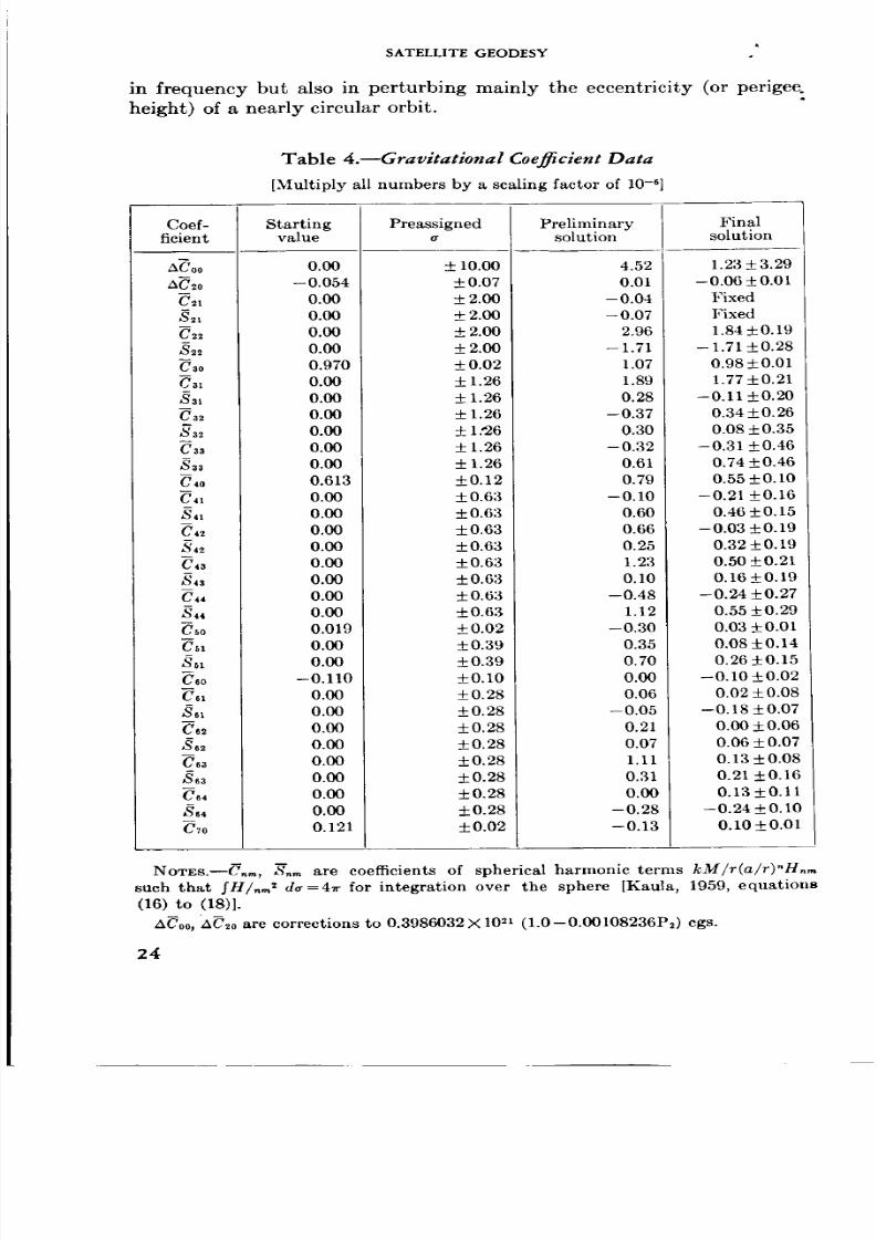
The harmonics listed in Table 4 were selected as having an rms antici-
pated effect on the satellite orbit of ___20 meters or more, using the
degree variances given by Kaula [1959].
As expected, the partial derivatives indicated poor separation of even-
degree harmonics of the same order rn, causing principally along-track
perturbations of frequency m (_-_). However, the effect of odd-degree
harmonics, especially third, was unexpectedly distinct, differing not only
23
8/7/2019 Significant Achievements in Satellite Geodesy 1958-1964
http://slidepdf.com/reader/full/significant-achievements-in-satellite-geodesy-1958-1964 32/170
SATELLITE GEODESY
in frequency but also in perturbing mainly the eccentricity (or perigee.
height) of a nearly circular orbit.
Table 4.--Gravitational Coefficient Data
[Multiply all numbers by a scaling factor of 10 -e]
Coef-
ficient
_00
AC_o
C22
$22
C32
_m
C33
J._33
C41
_,_41
C42
$42
C43
_43
C44
_44
C6o
C62
S62
C63
+_63
C64
S64
C7o
Startingvalue
0.00
-0.054
0.00
0.00
0.00
0.00
0.970
0.00
0.00
0.00
0.00
0.00
0.00
0.613
0.00
0.00
0.00
0.00
0.00
0.00
0.00
0.00
0.019
0.00
0.00
-0.110
0.00
0.00
0.00
0.00
0.00
0.00
0.00
0.00
0.121
Preassigned
ff
+ 10.00
___0.07
_2.00
_2.00
±2.00
±2.00
±0.02
± 1.26
± 1.26
± 1.26
± 1:26
± 1.26
± 1.26
±0.12
± 0.63
± 0.63
±0.63
±0.63
± 0.63
± 0.63
± 0.63
±0.63
±0.02
± 0.39
±0.39
±0.10
±0.28
±0.28
+__0.28
±0.28
±0.28
±0.28
±0.28
±0.28
±0.02
Preliminarysolution
4.52
0.01
--0.04
--0.07
2.96
--1.71
1.07
1.89
0.28
--0.37
0.30
--0.32
0.61
0.79
--0.10
0.60
0.66
0.25
1.23
0.10
--0.48
1.12
-0.30
0.35
0.70
0.00
0.06
-0.05
0.21
0.07
1.11
0.31
0.00
-0.28
--0.13
Final
solution
1.23 ±3.29
--0.06 ±0.01
Fixed
Fixed
1.84 ±0.19
- 1.71 ±0.28
0.98±0.01
1.77 ± 0.21
-0.11±0.20
0.34 ±0.26
0.08 ± 0.35
-0.31 ±0.46
0.74 ±0.46
0.55±0.10
-0.21 ±0.16
0.46 ± O. 15
-0.03 ±0.1(3
0.32±0.1(3
0.50 _+0.21
0.16±0.1 c
--0.24 ±0.27
0.55 ±0.2_
0.03 -4-0.01
0.08±0.14
0.26 ±0.1_
--0.10 ±0.0'
0.02±0.0t
--0.18 ±0.0:
0.00 + 0.0{
0.06 ± 0.0'
0.13 ±0.0_
0.21 ±O.D
0.13±0.1
--0.24+0.11
0.10 ±0.0
NOTES.--C,m, S,m are coefficients of spherical harmonic terms kM/r(a/r)"H,,,
such that fH/_,_ _ da=4_r for integration over the sphere [Kaula, 1959, equations
(16) to (18)1.
ACoo, AC_o are corrections to 0.3986032 X 10²¹ (1.0--0.00108236P2) cgs.
24
8/7/2019 Significant Achievements in Satellite Geodesy 1958-1964
http://slidepdf.com/reader/full/significant-achievements-in-satellite-geodesy-1958-1964 33/170
• CURRENT KNOWLEDGE OF EARTH'S GRAVITATIONAL FIELD
: For tesseral harmonic coefficients, initial values of zero were assumed;
for zonal harmonic coefficients, the values of Kozai [1962a] were used.
For the gravitational effects of the sun and moon, a similar disturbing
function was used [Kaula, 1962d]. All secular terms were retained, plus
periodic terms of more than 2X 10⁻⁵ amplitude, of which two to nine
were found for each orbit.
For the radiation pressure effect of the sun, the disturbing function
given by Kaula [1962d], was used. Because of the irregular effect of
the earth's shadow, the perturbations were not integrated analytically,
and a numerical harmonic analysis was applied instead. A harmonic
analysis interval of 15 days (or a minimum period of 30 days) was found
sufficient to reflect all variations in amplitude of more than 2X10 -5.
Partial derivatives were formed only for one parameter: the mean
reflectivity times the cross-sectional area.
For drag, the effect of an empirical atmospheric model was applied,
with density in the form [Jaechia, 1960]:
_h - h0(10)
In (10), S is the solar flux of 10.7- or 20-era wavelength, h is the
height above the earth's surface, and ¢ is the angle from the center of
the diurnal bulge, determined by
cos _b= {1, 0, 0}R3ff,*)R,(_)R3(×)l_qq/r (11)
where ,k* is the sun's longitude, e is the inclination of the ecliptic, and
x is the lag of the atmospheric bulge behind the sun.
The atmosphere was assumed to rotate with the solid earth and to
have the oblateness of a fluid. The customary assumption of the drag
force being proportional to the square of the velocity was made. The
force components that are radial, transverse, and normal to the satellite
and its orbital plane were used in the Gaussian equations of motion
[Brouwer and Clemence, 1961, p. 301], and numerical Fourier series were
developed for the effects on the Keplerian elements. In generating
these series, second-order effects on the angular elements that are de-
pendent on the secular motions due to the oblateness were included.With an anaJysi_ i,_le_al of 3 a ........ _,_n_ in amnlitude as small as
3 X 10⁻⁶ were obtained in M.
For satellites 1959al and 1959,/ the values of the parameters in (9)
that were determined by Jacchia [1960] were used. For satellite 1960L2,
c, _, and k were set equal to zero, and p0, m. H, b, n, and x were deter-
25
8/7/2019 Significant Achievements in Satellite Geodesy 1958-1964
http://slidepdf.com/reader/full/significant-achievements-in-satellite-geodesy-1958-1964 34/170
SATELLITE GEODESY
mined so as to fit the atmospheric models of Harris and Priester [1962].:
For 1959al and 19597, the Jacchia model absorbed most of the long-period
drag variations but did not fit variations characterized by periods of
less than 10 days. For 1960t_, the Harris and Priester model did not
reduce residuals significantly and had a negligible effect on the values
determined for the geodetic parameters, and hence it was omitted.
In computing the effects of arbitrary polynomials or the partial
derivatives with respect thereto, the second-order effects of the accelera-
tion based on the assu,mption of constant perigee height [equations (5)
to (14), O'Keefe et al., 1959; equation 2.100, Kaula, 1962c] were applied.
In the partial derivatives J with respect to the intermediate orbit
elements at epoch (equation 7), the effects of secular motions due to
oblateness were included [Kaula, 1961a, equation 49]. To ensure thatthe _+20-meter specification was met, the extension of Brouwer's theory
to periodic terms of order J22 by Kozai [1962b] was examined but was
found not to be needed.
In the final analysis of the orbit all the perturbations were added to
the osculating elements as determined from the preliminary orbit at
each observation. The long-period and secular perturbation_ that are
due to luni-solar attraction, radiation pressure, and drag by a specified
atmospheric model were omitted. For the orbital arc lengths of 10 to
20 days, it was found that these effects were adequately absorbed by an
arbitrary acceleration in the mean anomaly. Their inclusion made little
difference in the solutions obtained for tesseral harmonics or station
shifts--if anything, they may have distorted the results by shifting
computed satellite directions farther from those observed.
Data analysis.--As discussed in earlier papers [Kaula, 1961b, 1962a,
b], difficulties are created by (1) the nonuniform distribution of observa-
tions; (2) the similarity of effects on the observations of different gravi-
tational coefficients and station-position errors; (3) the inadequacy of
the atmospheric model; and (4) the prohibitive amount of computing
time which would be required by a solution that takes into account
serial correlation between different times. Three methods were used to
overcome these difficulties:
(1) Preassigning variance and covariance V for the starting values of
parameters to which corrections z are being determined so that the
solution becomes [Kaula, 1961a]
z = (MrW-IM+ V-1)-lMrW0-1f (12)
where W is the covariance matrix of the observations, M is the matrix
of partial derivatives in the observation equations, and f is the vector
of residuals.
26

8/7/2019 Significant Achievements in Satellite Geodesy 1958-1964
http://slidepdf.com/reader/full/significant-achievements-in-satellite-geodesy-1958-1964 35/170
* CURRENT KNOWLEDGE OF EARTH'S GRAVITATIONAL FIELD
(2) Assigning higher weight to the across-track than to tke along-track
component of an observation, as described by equation 3.
(3) Using arbitrary polynomials.
It was found that inclusion or omission of effects which were secularor of periods of more than a few days had very little influence on the
values determined for the station shifts or tesseral harmonics. The most
troublesome inadequacy was the inability of the empirical atmospheric
models to.explain orbital variations in the 1.0 to 0.1 cycle per day part
of the spectrum. The principal improvement which might be made
would be to utilize the correlation of corpuscularly caused density vari-
ations with the A_ index [dacchia, 1962].
It was found necessary to apply the device, specifying variance and
covariance for the starting values of the parameters, in order to avoid
absurdly distorted results due to the ill-conditioning caused by the non-
uniform distribution of observations and the inadequate accounting
for drag effects. For the stations on the Am., EASI, and JKM geodetic
systems, the 9 X 9 covariance matrix generated in the solution of Kaula
[1961c] was used. For the three isolated datums, the assigned covariance
matrices were based on assumed error ellipsoids of _+35-meter vertical
semiaxes in all three cases, and horizontal semiaxes of +_100 meters for
Au., __+200 meters for Ar., and +250 meters for H. The smaller un-certainty for the Australian system is based on the improvement of its
position by adjusting deflections of the vertical [Veis, 1961]. For the
zonal spherical harmonic coefficients of the gravitational field, the pre-
assigned variances were based on the uncertainties given by Kozai
[1962a], multiplied by 4. For the tesseral harmonics n, m=2,1 and 2,2,
the preassigned variance of (2.0X 10⁻⁶) 2was based on the order of magni-
tude of earlier determinations of J_ by Kozai [1961], Kaula [1961b], and
Newton [1962], except that C21 and S_ were held fixed. For the tesseral
harmonic coeff.cients of the third and higher degrees, the preassigned a's
in Table 4 were computed from the degree variances a__ {zXg} [Kaula,
1959]:
a2{C_ or _;_} = a: {z_g} (13)(n-- 1)2g_(2n_- 1)
The observational variance employed was (0.026 sec) 2 time and (9.2
sec) 2 direction for 12-day arcs of 1959al and 1959,1, (0.047 sec) _ time and(13.4 sec): direction for 20-day arcs of !960-2; (0.146 sec) _ time and
(43.8 sec) 2 direction for 10-day arcs of 1961_; and (0.047 sec) 2 time and
(13.4 sec): direction for 18-day arcs of 1961a_1. The principal criterion
used in determining the observational variances was the'x 2 test; i.e., the
quantity
27

8/7/2019 Significant Achievements in Satellite Geodesy 1958-1964
http://slidepdf.com/reader/full/significant-achievements-in-satellite-geodesy-1958-1964 36/170
SATELLITE GEODESY
s = (f_W-lf-z_/l_W-lf/n-p) (14):
should average 1 for several orbital arcs, where f is the vector of observa-
tion equation residuals; W is the covariance matrix of observations;
z is the vector of corrections to parameters; M is the matrix parameter
coefficients in the observation equations; n is the number of observa-
tions; and p is the number of free parameters. In forming the covariance
matrix W, observations in the same pass were treated as having the same
timing error.
The arc lengths used were chosen after some experimentation as giving
a reasonable compromise between magnitude of residuals and number
of observations.
The use of arbitrary polynomials was held to a minimum; i.e., the
only one used was a F variation in the mean anomaly.
In determining the estimated mean value and its standard deviation
from several orbital arcs of the same satellite, the weighting of a partic-
ular arc was considered to be proportionate to its degrees of freedom.
The computer program limited to fifteen the number of arcs that could
be combined at a time. In combining the results of several sets of
fifteen (or fewer) arcs, the weight ascribed to the mean of each set was
considered to be the inverse of its variance, or standard deviation squared.
In order that the final mean and standard deviation reflect as much aspossible any systematic differences which were functions of orbital
specifications, all sets were combined, with inverse-variance weighting,
into four groups: 1959al and 1959,7, twelve sets; 1960_2, two sets; 1961&,
one set; and 1961a_1, one set. The final means and standard deviations
given in Table 5 are the result of an inverse-variance weighted com-
bination of these four group solutions. However, for most of the
variables, the standard deviations from combining the four groups were
smaller than the standard deviations combining all sixteen sets at once,
primarily because the differences between the 1960L2 mean and the
1959a_ and 19597 mean were smaller than the scatter of 1959al and
19597 solutions about their own mean.
To avoid the tendency to prejudge the order of magnitude of the
solution, which is the main defect of the preassigned-variance technique,
some computer experimentation was tried in determining the amplitudes
of specified periodic variations, in place of harmonic coefficients, in
holding the reference orbit fixed, and in analyzing residuals. Applyingthese methods to one satellite at a time did not give as good results
as the preassigned-variance method, to judge by the scatter of solutions.
To apply them to data from more than one satellite simultaneously
required considerable program revision which did not seem worthwhile
28

8/7/2019 Significant Achievements in Satellite Geodesy 1958-1964
http://slidepdf.com/reader/full/significant-achievements-in-satellite-geodesy-1958-1964 37/170
CURRENT KNOWLEDGE OF EARTH'S GRAVITATIONAL FIELD
Table 5.---Gravitational Coefficient Solutions
[Multiply all numbers by a scaling factor of 10-e]
Coeffi-cient *
ACoo
AC2o
_;22
$22
C3o
_;32
$32
Cf33
C42
C43
C44
_'44
C61
C62
862
C63
863
C64
864
C7o
1959al 1959,_ 1960,_ 1961al
4.96
--0.06
1.30
--1.74
0.97
1.30
0.29
--0.14
0.490.36
0.83
0.68
--0.38
0.43
-0.10
0.52
0.18
0.29
0.120.11
0.02
--0.14
--0.06
--0.09
--0.01
--0.09
--0.04
--0.09
--0.02
--0.12
--0.00
--0.06
0.12
-8.88
--0.06
1.36
--0.76
0.96
1.62
0.99
--0.13
0.291.11
1.11
0.67
--0.38
0.53
--0.10
0.68
0.35
0.11
0.010.22
0.03
--0.02
--0.03
--0.08
--0.03
--0.02
0.05
--0.18
-0.10
-0.01
0.06
-0.09
0.12
--0.75
--0.05
1.99
--1.63
O.98
1.53
--0.10
0.29
0.380.42
0.89
0.61
--0.33
0.45
0.02
0.36
0.50
--0.00
--0.200.36
0.03
--0.01
--0.01
--0.04
0.00
--0.07
--0.01
-0.01
0.15
-0.08
0.06
-0.42
0.07
- 18.50
--0.29
1.80
--0.32
1.01
--0.96
--0.34
2.35
--0.162.36
0.43
--0.35
--0.48
0.39
0.03
--0.43
0.44
0.16
0.200.29
0.01
--0.63
0.23
1.10
--0.26
--0.49
--0.07
--0.07
-0.02
--0.06
--0.19
--0.30
0.09
1961a_!
-9.85
i 0.00
! 2.52
--0.89
0.97
1.18
0.46
--0.84
0.981.70
- 1.33
0.62
--1.00
0.45
0.47
0.06
0.17
I 0.42
--0.240.32
0.02
(b)
(b)
--0.10
--0.09
--0.06
0.05
0.01
(b)(")
-- 9.01
i).03
_).12
Weighted mean
-2.46_+2.36
--0.03 +0.02
1.88-+0.29
--1.38+_0.17
0.97 -+0.01
1.52 _+0.03
0.14_+0.16
--0.02_+0.26
0.42_+0.060.70 _+0.26
0.76 _+0.29
0.67 _+0.02
--0.33 _+0.01
0.37 _+0.15
0.01 _+0.02
0.35_+0.15.17_+0.02
0.41 _+0.03
i --0.01 _+0.080.18_+0.05
0.02 _+0.01
--0.13_+0.02
--0.01 _+0.01
--0.09 _+0.02
--0.05 _+0.08
--0.06_+0.01
0.01 _+0.01
--0.02 +0.03
O.15 -+0.01
--0.08-+0.01
--0.01 -+0.01
--0.03 _+0.07
0.12+0.01
C,_, and S,_ are coefficients of spherical harmonic terms kM/r/a/r) _ H,,_ such
that _H,, 2 da=4_r for integration over the sphere. 5C00 and AC_0 are corrections
to 0.3986032 X 10²_ (1.0 -0.00108236P2) cgs.
b No determinations of Cs_, S_!, C6,, Se, were made from 1961a51 because the
partial derivatives of the orbit with respect to these coefficients were all smaller thanthe criterion 0.1n 1-2 [Kaula, 1963a].
because this method has been applied extensively by Izsak [1963]. Other
changes tried and dropped as unnecessary were deleting orbital segments
for which observations are scanty and holding fixed the station shifts
29

8/7/2019 Significant Achievements in Satellite Geodesy 1958-1964
http://slidepdf.com/reader/full/significant-achievements-in-satellite-geodesy-1958-1964 38/170
SATELLITE GEODESY
obtained from the previous analysis of 1960L2 observations. The device
of weighting observations inversely as their density with respect to the:
phase angle (node-GST) was tried and dropped.
Results.--The analysis described above took much time to apply to
the large quantity of 1959al and 19597 data. The attempt to combine
solutions from different sets of arcs was not made until this analysis
had been completed. Consequently, the good agreement shown by
Table 5 between the results from 1960t2 on the one hand and from
1959al and 19597 on the other came as a pleasant surprise. The com-
bination of results is not as good, of course, as is suggested by the formal
standard deviations given in the table; in particular, the errors in dif-
ference of position between stations in North and South America--or
between stations in Europe, Africa, and India--which were held fixed
with respect to each other, are probably several times as great as someof the stated uncertainties. The good agreement is even more marked
for the spatial representations given in Figures 1 and 2; e.g., for the seven
® o
2O _o
%
•9 "o % 28\.o
'c-_o _ o o
eo
0 ,_o
%
Figure /.--Vanguard geoid. Geoid heights, in meters, referred to an ellipsoid of
flattening 1/298.24, determined from observations of satellites 1959c_, and
19597.
most extreme maximums and minimums in the Vanguard geoid of Figure
1, there are maximums and minimums in the Echo rocket geoid of Figure
2 agreeing within 10 ° in location and within 11 meters in magnitude.
The degree of independence in these solutions is fairly satisfying. The
orbits differ by 0.23 in inclination, and 0.16 in eccentricity; the arc
lengths used differed in a ratio of 5 to 3, and the observ_ttional weighting
differed in a ratio of 3 to 2. It would be very desirable, however, to
obtain comparable series of observations of a satellite of much higher
inclination.
30

8/7/2019 Significant Achievements in Satellite Geodesy 1958-1964
http://slidepdf.com/reader/full/significant-achievements-in-satellite-geodesy-1958-1964 39/170
CURRENT K.NOWLEDGE OF EAKTI_S GRAVITATIONAL
, p
lo _o - 1 to
0 eo _o 2 eo
Figure 2.--Echo rocket geoid. Geoid heights, in meters, referred to an ellipsoid
of flattening 1/298.24, determined from observations of satellite 1960,,.
The principal sources of systematic error likely to be common to
satellites 1959al, 195971, and 1960t_ seem to be (1) that the magnitudes
of the results will be influenced by the preassigned variances and (2)
that the relative positions of tracking stations on the same geodetic
datum may be appreciably in error.For a parameter whose effects are fairly distinct in periodicities, etc.,
from those of other parameters, it is implausible that its preassigned
variance could cause a correction that is too large or of wrong sign, but
it might cause a correction that is too small. However, the variance
actually used in the analyses is not the estimated squared magnitude of
the correction a2(c), but rather Na_(c), where N is the number of orbital
arcs in a set. Since N was always between 10 and 15, this seems to be
no more than a mild restraint preventing occasional ill-conditioned arcs
from obtaining absurdly large corrections beyond the range of linearity.
Distortion caused by the preassigned variances seems most likely to
occur in separating gravitational coefficients whose principal effects are
of the same period; i.e., coefficients J,= and J_l, such that m= 1 and
n-k is even. The most prominent set of such coefficients is J=, J_,
and Je_, all of which cause semidally variations of argument 2(12-0).
A way of removing some (but not all) of the influence of the preassigned
covariances would be to assume that what we have determined is not
the coefficients themselves but the amplitudes of semidaily variationsin the orbital elements; e.g., for the cos 2(12--0) term in the variation
of the inclination
ai - ai - ai -
Ai = .--'_'-029_-{-_ C cr.-{--_--_ 9 C,9_0L,'_ 0G'42 L,6_
(15)
31

8/7/2019 Significant Achievements in Satellite Geodesy 1958-1964
http://slidepdf.com/reader/full/significant-achievements-in-satellite-geodesy-1958-1964 40/170
SATELLITE GEODESY
The semimajor axis and the eccentricity have no semidaily variation.
If we omit the 1961_1 and the 1961a_1 results and assume that the simi-:
lar 1959al and 1959_/ orbits should be combined, we have two sets of
eight equations for three unknowns. Using values C_=1.315×10 -6,
_22 '_- -- 1.473X I0 -8, C42= 0.101X I0 -e, $42= 0.567X10 -6, C62= -0.009X
10 -6, Se2 =-0.I04>(10 -6 for the combined 1959al and 19597/ solution
(corresponding to Figure 1) and using values from Table 5 for 1960¢2 we
get the computed amplitudes of periodic perturbations in columns 6 and
Table 6.--Semidaily Perturbations o] Satellite Orbits
Satellite
(1)
1959al and
19597
combined.
1960_2 ....
Ele- aEl 0El 0El
ment ---=-- I _ --
(El) 0C22 aC_2 OC6_
(2__2_)3__L)(4) (5)M -2.92 036 574i 3.62- 5.89 3.83
oJ 1.68 12.21 --24.58
t-5.54 4.22 4.88M --0.04[ 0.001 -- 0.86
i 5.48- 5.08- 0.34-- 2.61
_o --2.59 / 20.861 7.66_ --5.07 -- 3.26
106X
Comp5Elc
(6)
- 3.93
5.33
1.20
- 7.76
- 12.05
10.81
- 4.76
-10.12
0S22
(7)
2.92
3.62
-- 1.68
5.54
6.04 I
5.48 I
2.59[
5.07
0E_A_I0S_2
(8)
- 0.3_
-- 5.89
--12.21
-- 4.22
0.00
-- 5.08
--20.86
3.26
0E10S6_
(9)
- 5.74
3.83
24.58
-- 4.88
0.861
-- 0.34
2.611
-- 7.66
106 ×
CompAE1,
(10)
-- 3.91
-- 9.12
-- 7.O9
-- 11.10-- 9.86
-- 10.76
-- 11.70
-- 7.07
10 of Table 6. Using these amplitudes as the observation equation
constants and solving by the rule of minimizing Y.(dAE1) 2 yields
C22 = 1.85X 10 -6
C42:0.05 _( 10 -6
C62 = 0.10X 10 -6
S22 = - 1.75)< 10 -6
$42 = 0.34 )< 10 -6
S62 : -- 0.22 X 10 -6
All the coefficients are increased over the mean in Table 5 except
$42, which hints of ill conditioning. However, it looks as though only
C62 and $62 might have been significantly reduced by the preassigned-
variance method.
The assumption that the relative positions of tracking stations on the
same datum should be known through triangulation networks with a
rms error of _+20 meters or less was based on standard methods of esti-
mating triangulation accuracy [Bomford, 1962, pp. 143-159], as is con-
firmed by the misclosures of large loops of triangulation: (1) 15 meters
in the 4000-km loop around the western Mediterranean [Whitten, 1952];
32

8/7/2019 Significant Achievements in Satellite Geodesy 1958-1964
http://slidepdf.com/reader/full/significant-achievements-in-satellite-geodesy-1958-1964 41/170
CURRENT KNOWLEDGE OF EARTH'S GRAVITATIONAL HELD
(2) less than 25 meters in the 10,000-kin loop around the Caribbean
- [Fischer, 1959]; and (3) within 15 meters for the 10,000-kin loop around
the Black Sea and Caspian Sea, through Turkestan, and connecting
in northwest India [Fischer, 1961].
The connections between the three northern hemisphere stations ofthe EASI system are closely associated with loops 1 and 3, and the con-
nections between the three northern hemisphere stations of the Am.
system are closely associated with loop 2. More in doubt are the posi-
tions of the stations in the southern hemisphere in Peru and South Africa,
which depend on long single arcs of triangulation. A test run was there-
fore made on all the 1960,2 data, in which the stations Arequipa (in
Peru) and Olifantsfontein (in South Africa) were assumed to be on sepa-
rate datums. The results of this test corroborated the assumption as to
triangulation accuracy; the station in Peru moved 24 meters with respect
to those in North America, while the station in South Africa moved 14
meters with respect to those in Eurasia. The changes in the gravitational
coefficients were insignificant--C_, from 1.99 to 2.11X10⁻⁶; S_, from
-1.63 to -1.60X10-e; (_31, from 1.53 to 1.49X10⁻⁶; C4a, from -0.33
to -0.28X10⁻⁶; etc.--and the maximum effect on any geoid height in
Figure 2 was 4 meters.
There still exists the possibility of errors in the local connection of
tracking stations to the triangulation systems, a matter in which betterstandardization of procedures is needed [Kaula, 1963b]. To check this
type of error for stations on the major datums we calculate the geometric
geoid heights corresponding to the final positions in rectangular coor-
_o
0
_o
_o
,i
_o
re
; 20.
35
t36
401 -9
0
2ii
Figure 3.--Combined geoid. Geoid heights, in meters, referred to an ellipsoid
of flattening 1/298.24, determined from observation of satellites 1959al, 1959_,
1960,2, 1961_1, and 1961a_1.
53

8/7/2019 Significant Achievements in Satellite Geodesy 1958-1964
http://slidepdf.com/reader/full/significant-achievements-in-satellite-geodesy-1958-1964 42/170
SATELLITE GEODESY
dinates and then compare these heights with the gravitational geoid
heights in Figure 3. To estimate the size of discrepancies to be expected, .
we have the geoid height variance of 1076 m s from autocovariance
analysis of gravimetry [Kaula, 1959] and a mean square height of the
satellite geoid of 466 m 2, obtained from the sum of the squares of the
coefficients in Table 5. If the station positions and the equatorial radius
were correct, the rms expected discrepancy between the geometric and
gravitational geoid heights due to the inability of the satellite orbits to
pick up the shorter-wave variations would be (1076-466) 1/2 = _+ 25 meters.
The results of the comparison are shown in Table 7. Applying the
mean correction of -[-31 meters yields a mean equatorial radius of
6,378,196_+11 meters and arms discrepancy of _+38 meters, which
implies arms radial position error of (382-252) '/2-- _+29 meters. Of
the stations on the major datums, the 60-meter discrepancy for San
Table 7.--Comparison o] Geometric and Gravitational Geoid Heights
Station Datum
Organ Pass ....
Arequipa ......
Curacao .......
Jupiter ........
()lifantsfontein _
San Fernando__
Naini Tal .....
Shiraz .........
Woomera ......
Tokyo .........
Villa Dolores___
Maul ..........
A Ill.
EASI
An.
JKM
Ar.
H
Geometric
geoid
height, m
-4
--16
-25
-18
+22
+117
-17
+14
+47
+54
+ 104
+54
Gravita-
tional
geoid
height, m
-10
-8
-10
-9
+5
+26
-41
-18
+24
+4
+4
-12
Discrepancy for
6,378,196 m
radius, m
+6
--8
-15
-9
+17
+91
+24
+32
+23
+50
+ I00
+66
Discrepancy for
6,378,196 mradius, m
-25
-39
--46
-40
-14
+60
-7
+I
--8
+19
+69
+35
NOTE.--Geoid heights referred to ellipsoid of equatorial radius 6.378,165 meters,
flattening 1/298.24.
Fernando causes suspicion of local connection error; however, there is
also a 69-meter discrepancy for Villa Dolores, which was free to move to
its correct position.
The solution in Figure 3 agrees with astrogeodetic [Fischer, 1961]
and gravimetric [Uotila, 1962] solutions, particularly in showing a more
pronounced negative in the western Atlantic. The discrepancies which
exist may in part be ascribed to the method of analysis of the terrestrial
data, since the agreement is appreciably better with the combination of
34

8/7/2019 Significant Achievements in Satellite Geodesy 1958-1964
http://slidepdf.com/reader/full/significant-achievements-in-satellite-geodesy-1958-1964 43/170
atq
CURRENT KNOWLEDGE OF EARTH'S GRAVITATIONAL HELI_
astrogeodetic, gravimetric, and satellite zonal harmonic data of Kaula
. [1961c], especially for western Europe.
• The reference flattening of 1/298.24 is used in Figures 1, 2, and 3
to facilitate comparison with the results of Kaula [1961c, 1963a]. The
flattening equivalent to the solution obtained for AC20 is 1/298.28. The
J2 equivalent is 1082.48X 10 -6.
In conclusion it can be said that better explanations are needed for
the systematic discrepancies indicated by Tables 5 and 7. However,
considering that the observations used herein depended on reflected
sunlight; that they were all made more than 3 years before the minimum
of solar activity; and that the orbital specifications are far from ideal,
the prospects are bright for extracting more information on the gravita-
tional field from more recent and anticipated satellites. It will be of
particular interest to push the analysis to a good determination of somesixth- or eighth-degree harmonics to see whether or not they corroborate
other indicators of a weak upper mantle.
REFERENCES
BOMFORD, G. : Geodesy, 2nd ed., 561 pp., Oxford University Press, London, 1962.
BROUWER, DmK: Solution of the problem of artificial satellite theory without drag,
Astron. J., 64, 378--396, 1959.
BROUWER, DmK; XND G. M. CLEm_NCE: Methods of Celestial Mechanics, AcademicPress, New York, 1961.
Fxscm_R, I.: A tentative world datum for geoidal heights based on the Hough ellipsoid
and the Columbus geoid, J. Geophys. Res., 64, 73-64, 1959.
FXSCl_ER, I.: The present extent of the astro-geodetie geoid and the geodetic world
datum derived from it, Bull. Geod., 61, 245-264, 1961.
H.CRAMUNDANIS, K. : Catalogue of precisely reduced observations, no. P-4, Smithsonian
Inst. Astrophys. 0bs. Res. in Space Sci., Spec. Rept. 95, 1962.
HARMS, I.; AND W. PmESTER: Theoretical models for the solar-cycle variation of
the upper atmosphere, NASA Tech. Note D-1444, 261 pp., 1962.
HENIZE, K. G.: Tracking artificial satellites and space vehicles, Advan. Space Sci.,
2, 117-142, 1960.
IZSAK, I. G.: Tesseral harmonics of the geopotential, Nature, 199, 137-139, 1963.
J^ccmA, L. G.: A variable atmospheric density model from satellite accelerations,
J. Geophys. Res., 65, 2775-2782, 1960.
JACCHIA, L. G. : Electromagnetic and corpuscular heating of the upper atmosphere,
Space Research, 3: Proc. Intern. Space Sci. Syrup., 3rd, Washington, North-Holland
Publishing Co., Amsterdam, in press, 1962.
KAULA, W. M.: Statistical and harmonic analysis of gravity, J. Geophys. Res., 64,
2401-2421, 1959.
KAULA, W. M.: Analysis of gravitational and geometric aspects of geodetic utiliza-
tion of ._t_l[ites_ Geophys. J., 5, 104-133, 1961a.KAVLA, W. M.: Analysis of satellite observations for longitudinal variations o[ the
gravitational field, Space Research, 2: Proc. Intern. Space Sci. Syrup., 2nd, Florence,
pp. 360-372, North-Holland Publishing Co., Amsterdam, 1961b.
35

8/7/2019 Significant Achievements in Satellite Geodesy 1958-1964
http://slidepdf.com/reader/full/significant-achievements-in-satellite-geodesy-1958-1964 44/170
SATELLITE GEODESY
KAULA, W. M. : A geoid and world geodetic system based on a combination of gravi-"
metric, astrogeodetic, and satellite data, J. Geophys. Res., 66, 1799-1812, 1961c.
KAULA, W. M. : Satellite orbit analysis for geodetic purposes (in Russian), Bull. Inst.
Theoret. Astron: Proc. Conf. on General and Practical Problems of Theoretical
Astronomy, Moscow, in press, 1962a.
KAULA, W. M.: Satellite orbit analyses for geodetic purposes, Proc. I.U.T.A.M.
Symp. Dynamics of Satellites, Paris, Springer-Verlag, Berlin, in press, 1962b.KAULA, W. M.: Celestial geodesy, Advan. Geophys., 9, 191-293, 1962c.
KAVLA, W. M.: Development of the lunar and solar disturbing functions for a close
satellite, Astron. J., 67, 300-303, 1962d.
KAULA, W. M. : Tesseral harmonics of the gravitational field and geodetic datum shifts
derived from camera observations of satellites, J. Geophys. Res., 68, 473-484,
1963a.
KAVLA, W. M.: A review of geodetic parameters; Paper presented at the Intern.
Astron. Union Symp., no. 21, The System of Astronomical Constants; to appear
in Bull. Astron., 1963b.
KozAi, Y.: Tesseral harmonics of the potential of the earth as derived from satellite
motions, Astron. J., 66, 355-358, 1961.
KozAI, Y. : The potential of the earth derived from satellite motions, Proc. I.U.T.A.M.
Symp. Dynamics of Satellites, Paris, Springer-Verlag, Berlin, in press, 1962a.
KOZAI, Y.: Second-order solution of artificial satellite theory without air-drag, Astron.
J., 67, 446-461, 1962b.
LASSOVSKY, K.: On the accuracy of measurements made upon films photographed by
Baker-Nunn satellite tracking cameras, Smithsonian Inst. Astrophys. Obs. Res.
in Space Sci., Spec. Rept. 74, 1961.
NEWTON, R. R.: Ellipticity of the equator deduced from the motion of Transit 4A,
J. Geophys. Res., 67, 415-416, 1962.
O'KEEFE,
J. A.;ECKELS, ANN; AND SQUIRES, R.
K.: The gravitational field of theearth, Astron. J., 64, 245-253, 1959.
UOTILA, IT. A.: Harmonic analysis of world-wide gravity material, Publ. Isostatic
Inst. Intern. Assoc. Geodesy, 39, 18 pp., 1962.
VEls, GEORGE: The positions of the Baker-Nunn camera stations, Smithsonian Inst.
Astrophys. Obs. Res. in Space Sci., Spec. Rcpt. 59, 1961.
VEIN, C.; HARAMUNDANIS, K.; SIMONS, L.; STERN, P.; AND _[AcDoNALD, J. E.:
Catalogues of precisely reduced observations, nos. P-1 through P-7, Smithsonian
Inst. Astrophys. Obs. Rcs. in Space Sci., Spec. Repts. 82, 1961; 85, 91, 95, 102,
104, 106, 1962.
VEIN, G.; AND WHIPPLE, F. L.: Experience in precision optical tracking of satellites
for geodesy, Space Research, 2: Proc. Intern. Space Sci. Syrup., 2nd, Florence,
pp. 17-33, North-Holland Publishing Co., Amsterdam, 1961.
WESTON, E.: Preliminary time reduction for the determination of precise satellite
positions, Smithsonian Inst. Astrophys. Obs. Res. in Space Sci., Rept. 41, 11--13,
1960.
WHITTEN, C. A.: Adjustment of European triangulation, Bull. Geod., 24, 187-206,
1(.)52.
55

8/7/2019 Significant Achievements in Satellite Geodesy 1958-1964
http://slidepdf.com/reader/full/significant-achievements-in-satellite-geodesy-1958-1964 45/170
The foUowin O paper was originally published in Journal of
Geophysical Research, rol. 69, no. 12, June 15, 196_, pp.2621-2630.
Tesseral Harmonics oJ the Geopotential and " "
Corrections to Station Coordinates
IMRE G. IZSAK
Smithsonian Astrophysical Observatory and Harvard College
Observatory, Cambridge, Massachusetts
INTRODUCTION
N THE PAST THREE YEARS numerous attempts have been made to
determine the small, large-scale, longitude-dependent irregularities in
the gravitational field of the earth from their effects on the motion of
artificial satellites. As often happens with methods still under develop-
ment, the first investigations on this subject were handicapped by an
oversimplified analysis of insufficient observational material; they led tocontradictory results and are already obsolete. It was only recently that
determinations based on optical data [Kaula, 1963a, b; Izsak, 1963] and
Doppler data [Anderle and Oesterwinter, 1963; Guier, 1963] have shown
encouraging agreement in the main features of the geopotential as inde-
pendently obtained by these authors. At the same time their results com-
pare favorably with those derived from an analysis of surface-gravity data
[Kaula, 1961b; Uotila, 1962]. Despite the reported progress, much work
must be done before we can reach definite conclusions about the longi-
tudinal dependence of the earth's gravitational field. The purpose of
this paper is to present new evidence concerning the subject. No at-
tempt will be made to evaluate critically the methods and results of the
authors mentioned above, for this would seem premature at this time.
The basic philosophy adopted in the present investigation is that a
statistical problem of such complexity should be considered from an
experimental rather than from a theoretical point of view. Instead of
trying to anticipate what might happen in the process of a very intricate
least-squares fitting, I think it preferable to carry out many different_glutigns under conditions as different as possible and then to choose the
best solution by comparing residuals, ,standard deviations, correlation
coefficients, etc. Questions regarding the convergence of the geopoten-
tial's development into an infinite series of spherical harmonics seem
37

8/7/2019 Significant Achievements in Satellite Geodesy 1958-1964
http://slidepdf.com/reader/full/significant-achievements-in-satellite-geodesy-1958-1964 46/170
SATELLITE GEODESY
irrelevant to me. A least-squares fitting of a finite number of terms can
merely give an approximation in the mean, which, in practical applica-
tions, is what we really are concerned with.
Our main interest is in the external gravitational field of the earth.
However, since the interpretation of satellite observations is affected by
the errors in the assumed coordinates of the Baker-Nunn camera stations,
it is imperative to improve the latter. Experimental evidence shows tbat
the correlations among harmonic coefficients and station coordinates are
generally weak, and those among corrections to the coordinates of
different stations are entirely negligible. Since the original connection
of the stations to major geodetic systems proved to be unreliable in
several instances, I decided to treat the 12 tracking stations individually.
COMPUTATIONAL PROCESS
The analysis of the observations begins with a painstaking computa-
tion of satellite orbits.
DOI 3, our differential orbit improvement program [Gaposchkin, 1964],
accounts analytically for the first-order short-period perturbations result-
ing from the oblateness and for the long-period perturbations caused by
the equatorial unsymmetry of the earth, as well as for hmar perturba-
tions with biweekly periods. Secular perturbations of gravitational
origin, the effect of atmospheric drag and solar radiation pressure, how-
ever, are as a rule determined empirically in the process of least-squaresfitting. The length of an orbital arc represented by a single set of mean
orbital elements varies between one and four weeks, depending on the
particular object; in such a time interval there are 60 to 500 observations.
On completing the computations, DOI 3 produces for each observation
a binary card that contains among other useful information the sidereal
time at Greenwich 0_, the along-track and across-track residuals dU_
and dlV, of the observation, as well as the instantaneous values M_, a_, e,,
I,, _f, and _ of the mean orbital elements. The binary cards pertain-
ing to several satellites in several time intervals are collected, and their
content is put on a magnetic tape, which will serve as input in the
subsequent analysis.
The residuals dU_ and dW_ comprise, besides components not suffi-
ciently accountable, the positional and timing errors of the Baker-Nunn
observations, the effect of the tesseral harmonics in the geopotential,
and the effect of small errors in the adopted station coordinates. By
analyzing many thousand observations one can arrive at reasonable
least-squares estimates of the tesseral harmonics' numerical coefficients
and of the corrections to the station coordinates. This is the purpose
of the tesseral harmonics and station coordinates program, a brief
description of which follows:
38

8/7/2019 Significant Achievements in Satellite Geodesy 1958-1964
http://slidepdf.com/reader/full/significant-achievements-in-satellite-geodesy-1958-1964 47/170
TESSERAL HARMONICS OF THE GEOPOTENTIAL
Let the geocentric position vector of a satellite as computed by DOI 3
• .be denoted by ro and a station vector as used in the computations be
Re; the corresponding topocentric position vector of the satellite is 0c=
r_- R_. If the correction to be applied to the station vector is dR = R- Re,
and the perturbations caused by the hitherto neglected tesseral harmonics
are given by dr=r-to the corresponding change in the topocentric posi-
tion vector will be do =dr-dR. Having only angular residuals at our
disposal, we disregard the line-of-sight component of this vector by
projecting it onto the directions of the along-track and across-track unit
vectors ev and ew. For the angular corrections in these directions we
have then
du = du _- du" dw = dw _- dw" (1)
where
and
du,-_-p-_ev.dR dw,=p-lew.dR (2)
du_=p-lev.dr dwh=p-lew.dr (3)
The positions of the Baker-Nunn stations [Veis, 1961, 1963a] being
given in an earth-fixed rectangular coordinate system X, Y, Z, we put
dR=ex dX+er dY+ez dZ (4)
Here the unit vector ex lies in the intersection of the equator with the
meridian of Greenwich; ez points toward the north pole; and er is
perpendicular to both of them.
The explicit representation of the vector dr is much more involved,
of course. It requires the elaboration of a perturbation theory for the
tesseral harmonics in the geopotential, a topic that will be touched upon
below. At present it suffices to say that any perturbations of the orbital
elements result in a vectorial displacement,
Or Or Or Or Or • Ordr = _. dM +-- da +-z- de+-z_ dI +-z- d_+-_ d_2 (5)o2vl oa o e o l o_o o_1
and that the perturbations in question are linear in the numerical co-
efficients of the tesseral harmonics. Full details concerning equations 1
thro_gh 5 were given in an earlier paper [D_sak, 1962].
In this way we obtain the observation equations
and
To be minimized is
du_ = du_ _- du_" = d U t
dw, - dw**- dw," = dW:
[(dU,-du,)_+ (dW,-dw,) _]i
(6)
39

8/7/2019 Significant Achievements in Satellite Geodesy 1958-1964
http://slidepdf.com/reader/full/significant-achievements-in-satellite-geodesy-1958-1964 48/170
SATELLITE GEODESY
where the summation is extended over the available observations of a
number of satellites at all participating stations. An earlier version of..
the program had the facility of applying different weights to the along-
track and across-track residuals, but the advantages of such an approach
seemed rather dubious in practice.
Concerning the perturbation theory for tesseral (and sectorial) har-
monics I confine myself to a few remarks. The disturbing function,
which determines Lagrange's equations for the variation of orbital
elements and thus the perturbations of the latter, is written in the form
R=# (a_'/r _+1) • (C,m cos mXq-Sn,_ sin mX)Pn_(sin _)
-- m_l
the adopted definition of the Legendre associated functions being
P,m(x) = (1 - x 2) m/2dmP,(x)/dx m
To utilize Lagrange's equation, we must develop the disturbing function
in terms of the orbital elements. This is conveniently done in two steps.
We note first that any rotation of the X, Y, Z coordinate system
induces a linear transformation of the nth-degree spherical harmonics
[Wigner, 1959], while the elements of the transformation matrix are
easily calculated as functions of the Eulerian angles of rotation by means
of the corresponding Cayley-Klein parameters. Let the X' and Z' axis
of a new coordinate system point toward the perigee and pole of the
satellite's orbit, so that the Eulerian angles coincide with _-0, I, and _.
In this system the polar coordinates of the satellite are k'=v and ¢/=0;
therefore the spherical surface harmonics degenerate into trigonometric
functions. Implementing these considerations we arrive at the expansion
n
P_m(sin _o) exp (im),)= x-_ _. j ....Z.¢lx.,_ z • exp {i[(n-2j)(v--boa)--bm(_2-O)]}
where
(n+m)! " "
K,,,'=2,j[(n_j)[" _(- 1)k[2n-2j][ 23 ]_,,_.¢.[ k J[n-m-kJ
(7)
3,=cos(I/2), a=sin(I/2), u=m-n+2j-t-2k, and the range of the k
summation is
max {0, n--m--2j} <k<min {2n--2j, n-m}
The polynomials (7) have the symmetry
K..,J(_/1 a) = (- l)"-"K.m--_(al _/)
4O

8/7/2019 Significant Achievements in Satellite Geodesy 1958-1964
http://slidepdf.com/reader/full/significant-achievements-in-satellite-geodesy-1958-1964 49/170
TESSERAL HARMONICS OF THE GEOPOTENTIAL
In'the second step, the functions
". r-"-1 exp [i(n-- 2j)v]
'are to be developed into a Laurent series of exp (/M), a process that
invokes the well-known Hansen coefficients from celestial mechanics.
This and related subjects were dealt with recently [Izsak et al., 1964].
For the actual computation of the effect of tesseral harmonics on the
orbital elements, we used a program that William M. Kaula of the
Goddard Space Flight Center kindly made available to us; its mathe-
matical formulation has already been described by Kaula [1961a]. Once
given the orbital elements o, e, and I, this program yields for the several
harmonics--apart from the at-this-stag_unknown numerical coefficients
C,_ and S,=--the perturbations dM, • •., d_2 in the form of trigonometric
polynomials. Three terms are used if n is even, and four if n is odd.
Thus, for instance, the effect of the second-, third-, and fourth-degree
harmonics upon each orbital element is represented by a total of 54
trigonometric terms. The complete expressions for the perturbations are
d U $1lll _ll m= _(CnrapM -_S.,nqx_ )
dfl = _(C,,_pe"" q-S,,,_qa "m)
(8)
the symbols pM "m, qM "m, ''', p_"m, qo "m standing for the trigonometric
polynomials given by Kaula's program. As examples, pertaining to
the mean orbital elements a=8306.8 kin, e=0.16446, and 1=32.883 ° of
the satellite 1959a_ (Vanguard 2), we choose
pM _= 4.008 sin [2o_q-2M-t-2(_2--0)]
-- 2.979 sin [2(f_-- 0)]
--0.025 sin [--2_--2Mq-2(f_- 0)]
and
qas'= --2.255 cos [--o0A-(1_--0)]
-}-5.481 cos [w-}-(l_-- 0)]
--1.113 cos [-w--M-]-(_-- 0)]
.... r...a-_(i2--O)]--O..tOO COS t_, i --- , _ ..
As a matter of fact, Kaula's program was adapted to fully normalized
spherical harmonics, the integral of whose square over the unit sphere is
41

8/7/2019 Significant Achievements in Satellite Geodesy 1958-1964
http://slidepdf.com/reader/full/significant-achievements-in-satellite-geodesy-1958-1964 50/170
SATELLITE GEODESY
4r. The relation between the coefficients C_,,, S,m of the ordinaryl and
C,,., S._ of the fully normalized, spherical harmonics is
Cnm = N_mC_m S.m = N_mSnm
where
N.o = (2n+ 1)1/2
V2(2n + l )(n-m) II 1/2N._: L _ i (m_ o)
Let us now return to the observation equations 6. They are set up
as follows. Comparison of (3) and (4) gives for the station that secured
the observation
du_=u x dX+u r dY+u z dZ
dw_=w x dX +w r dY+w z dZ
where
u x = p-l(ev, ex), ..., w z = p-_(e w. ez)
As to the harmonics, from (2) and (5) we have
du_=u M dM+u a da+u _ de+u _ dI+u _ d,o+u _ dft
dw _= O.dM+w _ da+w _ de+w r dI+w _ do,+w _ dft
with the abbreviations
u M= p-l(e v" Or/OM),..., w _= p-l(e w" OrOft)
Then, using (8) and collecting terms that belong to the same harmonic,
we get
dub= _¢(u:mC,,,+u:mS,,,)
n,m
--_/W nmc _W nmgd wh- X.I k c nm'l- S Onrn.I
where
u c nm _- U M p M n ra-Jf- . . . -3l-u_p_n mu,s n m = U M q Mn m 2f- . . . D- ?2,flft n m
Wc, " = w_p d,_ + . . . --_-wnpf_ n mw,sn m = Wa q an m+ . . . -._ wfl qu n m
Once the observation equations are set up, they are solved by the
computer using standard least-squares techniques. In its present version
our program can simultaneously handle up to 150 orbital ares of 10
different satellites; this corresponds to about 20,000 individual observa-
42

8/7/2019 Significant Achievements in Satellite Geodesy 1958-1964
http://slidepdf.com/reader/full/significant-achievements-in-satellite-geodesy-1958-1964 51/170
T_SSm.Cta_MONICSFTHEGEOVOTENTI_
tions. ° The selection of the unknowns to be solved for is arbitrary.
. Their number, however, is limited to 44. Of these unknowns not more
"than 38 may be tesseral-harmonics coefficients, and not more than 36
may be corrections to station coordinates. The printout of the program
has been devised to give detailed information concerning the intricateleast-squares process under discussion. Its main features are:
(1) A list of the original (DOI 3); the stations--improved (if any);
the harmonics--improved (if any) ; and the improved residuals
dU_ dW_
_U_'=dUc4-du_" _W/=dWc4-dw_"
5U__= d U_- dus k _W_ h= dW_- dw_h
and
_U_=dU_-du_ $W_=dW_-dw_
(2)
and
The mean values
.,v -1_/22N)-'
n "j:/22N)-' _ [(_U,)2+ (_W,)2]__1
of the original and of the improved residuals per orbital arc, as well as
for all the observations. We call their ratios the respective improve-
ment factors of a solution.
(3) The least-squares estimates of the fully normalized tesseral and
sectorial harmonics coefficients and of the corrections to station coor-
dinates together with their standard deviations.
(4) The matrix of the correlation coefficients, that is, the normalized
inverse matrix of the normal equations.
DATA ANALYSIS
As indicated by the foregoing description of the computational proc-
ess, the mathematics involved is rather straightforward; the difficulty
of the problem lies in the analysis of real data. First of all, the informa-
tion contained in the original residuals is contaminated by unaccountable
effects with a total that is significantly larger than the well-estabfished
accuracy of the observations: 2 seconds in the across-track and 3 seconds
in the along-track direction. Second, while the perturbations caused
43

8/7/2019 Significant Achievements in Satellite Geodesy 1958-1964
http://slidepdf.com/reader/full/significant-achievements-in-satellite-geodesy-1958-1964 52/170
SATELLITE GEODESY
by the presence of the various spherical harmonics are continuous func-
tions of time, optical observations necessarily result in discrete data"
of a distribution that, for a single orbital arc, is often anything but
uniform. This situation, though especially troublesome in case of per-
turbations with high frequencies, is comparatively harmless so far as
station coordinates are concerned. Third, the effect of the different
harmonics is not very much different in size and, for some terms, not
even in shape. Therefore the perturbations caused by the various
harmonics are hard to separate, a fact borne out by eventually consider-
able correlations among the computed values of the unknowns. About
the only thing one can do to minimize the influence of these disadvanta-
geous circumstances is to use a huge number of observations of several
satellites with a variety of orbital elements, particularly with different
inclinations. The self-explanatory Table 1 constitutes a breakdown ofthe 15,191 observations on which this analysis is based.
Table 1.--Observational Material
Satellite I, deg
1959_1, Vanguard 2 ........ 32.9
1959a_, Rocket of .......... 32.919597, Vanguard 3 ......... 33.4
196151, Explorer 9 ........ 38.9
1962a_1, Telstar 1 .......... 44.8
1960_2, Echo 1, rocket ...... 47.2
1962_uL, Anna 1B .......... 50.1
1961o_, Transit 4A ......... 66.8
1961o2, Injun 1--Greb 3 .... 66.8
1961a$_, Midas 4 .......... 95.9
0.165
0.183
0.189
0.115
0.242
0.012
0.007
0.008
0.008
0.011
a, km
8301
8492
8496
7985
9672
7972
7508
7318
7319
10005
Arcs
15
2
12
16
3
34
3
13
7
6
Number of
observations
2091
229
1824
2446
269
4324
296
971
494
2247
In the present computational approach, we need the coordinates of
the Baker-Nunn camera stations in some uniform rectangular system.
The method of reducing the fundamental geodetic coordinates of the
stations, based on field surveys and referred to five different geodetic
datums to such a system, has been given by Veis [1961]. The actual
values used in our computations, however, come from later, yet unpub-
lished, work of his. They were determined on the basis of improved
geodetic information available June 15, 1962, and (instead of the inter-
national ellipsoid) reduced to the ellipsoid (recommended by Kaula) withthe characteristics aE=6378.165 km and f=1/298.3. For the sake of
easy reference, we list in Table 2 the initial coordinates of our tracking
stations as derived by ¥eis.
44

8/7/2019 Significant Achievements in Satellite Geodesy 1958-1964
http://slidepdf.com/reader/full/significant-achievements-in-satellite-geodesy-1958-1964 53/170
TESSERALARMONICS OF THE GEOPOTENTIAL
Table 2.--Observing Stations
1. Organ Pass .....
2. Olifantsfontein__
3. Woomera .......
4. San Fernando___
5. Tokyo .........
6. Naini Tal ......
7. Arequipa .......
8. Shiraz .........
9. Curacao ........
10. Jupiter .........
11. Villa Dolores ....12. Maul ..........
X, km
-- 1535.702
5056.123
--3983.602
5105.623
--3946.522
1018.135
1942.762
3376.872
2251.841
976.319
2280.645--5466.118
Y, km
--5167.026
2716.523
3743.226
-555.194
3366.453
5471.207
- 5804.082
4404.022
-5816.928
-5601.410
-4914.512
-2404.068
Z, km
3401.108
-- 2775.799
--3275.656
3769.670
3698.855
3109.519
-- 1796.838
3136.250
1327.236
2880.311
--3355.441
2242.437
Datum
l
Am.
Eu.
Aus.
Eu.
Jap.
Eu.
Am.
Eu.
Am.
Am.
Arg.
Am.
Number of
observations
1826
1742
2023
1315
965
161
931
1123
831
1458
1276
1540
The satellite observations set forth in Table 1 have been used recently
in a great variety of computer runs. In some cases the required machine
time was well over an hour. There is little point in giving a full account
of the numerical results obtained. Instead, we select samples of them
in the form of tables that we think are pertinent to the problems under
discussion. All (fully normalized) harmonics coefficients will be expressed
in units of l0 -6, and the station corrections will be given in meters.
Throughout the computations we used the value # = GM = 3.986032 × l 0 :°
cm 3 sec -2 recommended by Kaula.
Table 3 shows how futile it is to use a single satellite even for the
determination of one pair of coefficients. The results per satellite are
incompatible, probably because the effect of the several harmonics
Table 3.--Second-Degree Solutions per Satellite
(Sealed by 10 6)
Satellite
1959al .......
19597 ........
1961_1 ........ !
1960t2 .........
|961m ........
1961o2 ........
1961a$, .......
All ten .......
_2
0.97 _ .08
1.22 _+.10
1.50 _+ .06
1.51 _+ .03
0.81 _+ .04
0.85 + .t_
2.29 ± .05
1.08 ± .02
S22
--2.17 + .08
--2.32_+.10
--1.64_+.06
-- 1.37 _+ .03
-- 0.52 -+ .04
--0.52 4- .05
--0.89 4-_.02
Residuals, _e
Original
14.27"
13.53
15.56
16.02
23.61
24.36
9.84
15.67"
Improved
12.95"
12.49
13.63
12.67
20.43
21.50
7.99
13.86"
45

8/7/2019 Significant Achievements in Satellite Geodesy 1958-1964
http://slidepdf.com/reader/full/significant-achievements-in-satellite-geodesy-1958-1964 54/170
SATELLITEEODESY
averages out differently according to the inclination of the objects. The
considerable differences in the mean angular residuals result primarily _
from the variety in the mean topocentric distances of the objects.
Table 4 illustrates the interaction of harmonic coefficients and station
corrections in a least-squares adjustment. In the first run only theharmonics up to the third degree were considered unknown; in the second
only the stations were varied. In the third and definitive run these
two problems were solved simultaneously. Clearly, the presence of tes-
seral harmonics influences the computed station coordinates much more
than small errors in the latter affect the computed harmonic coefficients.
The most conspicuous correlation coefficients among harmonics and
Table 4.--Third-Degree Solutions ]or Harmonics (Scaled by I0 _) and
Corrections to Station Coordinates (in meters)
CmSm 1.03 -1.14 1.02+.02 -1.13_.02
C31 S31 1.02 --0.32 1.35±.02 -0.18+.02
C_2 S_2 0.30 -0.45 0.35±.03 -0.73_.03
Ca3 $33 -0.31 0.99 -0.37 ±.04 1.01 ±.04
dX t dY1 dZ, -10 19 51 -40± 5 34± 5 -20± 5
dX, dY_ dZ2 31 64 --10 11± 5 --26± 5 --32± 6
dX3 dY3 dZ3 2 -20 13 -67± 4 -16± 4 10± 4
dX4 dY, dZ, 42 --72 10 -24±11 -34± 8 68± 8
dXs dY6 dZ6 --47 -89 -41 -101± 7 -80± 7 12± 8
dX6 dY6 dZ6 49 --64 84 44±16 -76±26 75+20
dX, dY, dZ7 --59 -44 -65 42± 7 --1± 8-103± 8
dX8 dY8 dZ8 77 --39 115 33± 7 --40+_ 7 59± 7
dX9 dY9 dZ9 -102 --55 --39 --10± 7 6± 9 --64+__ 8
dX1odY1odZlo -21 5 0 -41+_ 5 5± 6 -36± 6
dXl, dY,idZ,l -23 --43 9 --19_+ 6 -53± 7 --21± 7
dXl2dY,2dZ,2 53-152-138 37± 6-152± 5-163+_ 6
Improved
residuals 13.03" 14.85_ 12.11"
stations are ($32, dY,)=-0.25 and (Sin, dX,o)=0.25 and those among
the coordinates of different stations turn out to be (dX,, dY,)= -0.07
and (dX10, dY,2)=O.07. These data refer, of course, to the third run,
whose results concerning the station coordinates we regard as the best
the present version of our computer program can yield in conjunction
with the observational material used in this work. A generalization of
the program now under development will be indicated below.
At this point it is interesting to compare the results of the third run
with those obtained by Kaula [1963b] and Veis [1963c], who were both
using dynamical methods. In addition, we consider the purely geo-
metrical method of simultaneous observations, initiated and pursued at
46

8/7/2019 Significant Achievements in Satellite Geodesy 1958-1964
http://slidepdf.com/reader/full/significant-achievements-in-satellite-geodesy-1958-1964 55/170
• TESSERAI. HARMONICS OF TH]E GEOPOTENTIAL
the Smithsonian Astrophysical Observatory by Veis [1963b]. This tech-
oique permits the determination of two components 9_ and g2 of relative
displacement of tl_.e participating stations, perpendicular to the direction
of one station as seen from the other. Simultaneous observations have
already been succe_ful in tke instance of four pairs of neighboring sta-
tions, thus providing a valuable check on results arrived at by dynamical
o4
: : :
g
3• .,. 91
g2
2: : : i :_g !
. 0
o4/
Direction 1 to 10
( 2602 km )
g2
.0 3
3
; :_ gl ; O
Direction 7 to 9
(3139 km )
g2
: : , • q4
2 _
: ; I,-91
Direction 7 to 11 Direction 9 to 10
( 1826 km) (2021 kin)
ScaleO 50 100m
I . . , , I , , , , li
Figure/.--Comparison of satellite results for the relative direction of Baker-Nunn
camera stations 1 ° [Veis, 1963b]; 2 ° [Kaula, 1963c]; 3 ° [Veis, 1963c]; 4 °, Izsak,
Table 4.
47

8/7/2019 Significant Achievements in Satellite Geodesy 1958-1964
http://slidepdf.com/reader/full/significant-achievements-in-satellite-geodesy-1958-1964 56/170
SATELLITEEODESY
methods. Figure 1 compares these results. The origin of the individual
diagrams corresponds to the assumed direction of the respective stations;
Small circles represent relative displacements according to l ° [Veis,
1963b], where error ellipses are also given; 2° [Kaula, 1963b]; 3° [Veis,
1963c]; and 4°, our Table 4.The average agreement of the geometric results, 1 °, seems to be best
with the dynamical results, 4 °. In case of the direction of Arequipa-
Villa Dolores (7-11), the discrepancy between the determinations 2°
and 1° is so striking as to call for a careful investigation.
During the experimental phase of this work the harmonic coefficients
were computed in a variety of combinations. The purpose of such
numerical experiments was merely to establish the capabilities of our pro-
gram. We soon concluded that although the individual coefficients C_
and Sn,_ may vary significantly from run to run, the combined contribu-
tion of the several harmonics to the gravitational field of the earth is
Table 5.--Fourth-, Fifth-, and Sixth-Degree Solutions for Harmonics
(Scaled by 10 6)
C_2 Sm 1.06 -0.73 1.08 -0.70 1.17±.02 -0.95_.03
C31 S3t 0.88 -0.26 0.84 -0.21 0.81 +.02 -0.25 ±.02
C3_ S, 0.22 -0.36 0.30 -0.31 0.24+.03 -0.25±.03
C33 Ssl --0.30 0.79 --0.53 0.87 --0.50___.04 0.93 ±.04C,tS_t -0.18 -0.24 -0.19 -0.20 -0.18___.01 -0.25±.01
C_2 S,_ -0.16 0.52 -0.19 0.46 -0.11 ±.02 0.23 ±.02
C_3 S,_ 0.34 -0.08 0.32 -0.08 0.28+.02 -0.08 ±.02
C_, S,, 0.06 0.59 0.20 0.57 -0.08 +_.05 0.29 ±.06
C51 S_, -0.12 0.20 -0.09 +.01 0.19 ±.01
C6_ $6_ 0.30 -0.49 0.31±.03 -0.50 ±.03
C_, Ss_ -0.91 0.17 -0.72+.05 0.11 +.05
C6, $6_ -0.21 0.53 -0.18 +.06 0.51 ±.06
C55 $55 0.17 -0.35 0.18+_.10 -0.42±.10
C6t $61 -0.01 4-.01 0.13 ± .01
C6_ S_2 0.16 +.02 -0.37 ±.02
C6s $6_ 0.14 ±.02 -0.17 ±.02
C6, Se, -0.20 ±.04 -0.41 ±.05
C65 $66 -0.40 ±.04 -0.28 ±.04
C66 See -0.53 ±.08 -0.41 ±.08
Improved residuals 12.50" 12.27" 12.10"
rather well determined by sufficiently rich observational material. Table
5 is a compilation of recently obtained fourth-, fifth-, and sixth-degree
solutions for harmonics, the last of which we regard as the definitive
one. There seems little justification at present for going beyond sixth-
degree terms. The standard deviations of the computed coefficients,
48

8/7/2019 Significant Achievements in Satellite Geodesy 1958-1964
http://slidepdf.com/reader/full/significant-achievements-in-satellite-geodesy-1958-1964 57/170
. TESSERAL HARMONICS OF THE GEOPOTENTIAL
• whatever their significance, increase systematically with the index m, so
that they are largest for the sectorial terms. We enumerate here only
the most notable correlation coefficients:
(C,.,, C,2)=0.72 (Cm, C62)=0.55
<C33,C53)=0.36 <$3_,S_>=0.36
(C4,,C6,)= -0.38 <S,,,,$6,> -0.36
(C4_,Ce_)=0.61 (S,2,Se2)=0.63
(C,4, Ce4)=0.65 ($44, ,S_4>=0.67
To facilitate the visualization of numerical results, level curves of
geoid heights pertaining to our sixth-degree solution are plotted in Figure
2. The reference ellipsoid of oblateness 1/298.28 and the purely latitu-
dinal deviations from it are defined by the zonal harmonics coefficients of
Kozai [1962]. The most interesting deviations of this figure from that
in Izsak [1963] and Kaula [1963b] occur over the Atlantic and North
Africa; their reality, however, cannot be ascertained without further
evidence.
Extensions of the present computer program are feasible in a numberof ways. First of all, one could increase the number of unknowns to 52,
so that a simultaneous solution for the 12 stations of our network and
second-, third-, and fourth-degree harmonics would become possible.
Or, wishing to bring about a better separation of the geometric and
dynamical part of the problem, one might be inclined to iterate previously
obtained solutions. For instance, one could start with the results of the
third run in Table 4, take its improved residuals and use these in a solu-
tion for higher-degree harmonics. The effect of the harmonics thus
derived, in turn, would be subtracted from the original residuals when
starting a new solution for the stations.
Appendix.--Normalization Coe_cients
nm Nn,n n?n Nn,n
22 0.64550 51 0.85635
52 0.16183
31 1.0801 53 0.033034
32 0.34157 54 0.0077863
33 0.13944 55 0.002462241 0.94868 61 0.78680
42 0.22361 62 0.12440
43 0.059761 63 0.020734
44 0.021129 64 0.0037855
65 0.00080707
66 0.00023298
49
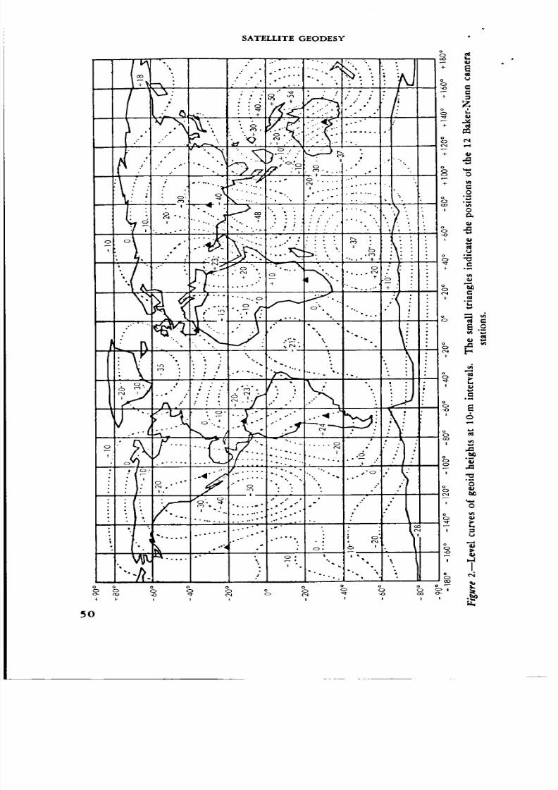
8/7/2019 Significant Achievements in Satellite Geodesy 1958-1964
http://slidepdf.com/reader/full/significant-achievements-in-satellite-geodesy-1958-1964 58/170
SATELLITE GEODESY
5O

8/7/2019 Significant Achievements in Satellite Geodesy 1958-1964
http://slidepdf.com/reader/full/significant-achievements-in-satellite-geodesy-1958-1964 59/170
!w
D
4 TESSERAL HARMONICS OF THE GEOPOTENTIAL
Acknowledgments.--This work was supported in part by grant NsG
'87-60 from the National Aeronautics and Space Administration. I am
much indebted to W. M. Kaula for helpful discussions on the subjects,
as well as for his furnishing me with one of the basic subroutines. The
complex computer programs used in this investigation are the skillful
work of Mrs. Gladys Johnson, E. M. Gaposchkin, and W. L. Joughin.
Figure 1 is based on the computations of A. Girnius.
REFERENCES
ANDERLE, R. J.; AND C. OESTERWINTER: A preliminary potential for the earth from
Doppler observations on satellites, paper presented to Cospar, Warsaw, 1963.
GAPOSCHKIN, E..XI. : A differential orbit improvement program, Smithsonian Aslro-
phys. Obs. Spec. Rept., in press, 1964.GVmR, W. H.: Determination of the non-zonal harmonics of the geopotential from
satellite Doppler data, personal communication, July, 1963, also Nature, 200(4902),
124-125, 1963.
IzsAx, I. G.: Differential orbit improvement with the use of rotated residuals, Space
Age Astronomy, edited by A. J. Deutsch and W. B. Klemperer, Academic Press,
New York and London, 1962.
IZSAK, I. G.: Tesseral harmonics in the geopotential, Nalure, 199, 137-139, 1963.
"[ZSAK, I. G.; J. M. GERARD; R. EFIMBA; AND _[. P. BARNETT: Construction of
Newcomb operators on a digital computer, Smithsonian Astrophys. Obs. Spec. Rept.
160, 1964.
KAULA, W. M. : Analysis of gravitational and geometric aspects of geodetic utilization
of satellites, Geophys. J., 5, 104-133, 1961a.
KAVLA, W. M.: A geoid and world geodetic system based on a combination of gravi-
metric, astrogeodetic, and satellite data, J. Geophys. Res., 66, 1799-1811, 1961b.
KAVLA, W. M.: Tesseral harmonics of the gravitational field and geodetic datum
shifts derived from camera observations of satellites, J. Geophys. Res., 68, 473-484,
1963a.
KALTLA, W. :Xl.: Improved geodetic results from camera observations of satellites,
J. Geophys. Res., 68, 5183-5190, 1963b.
KozAI, Y.: Numerical results from orbits, Smilhsonian Astrophys. Obs. Spec. Rept.
101, 1962.
UOTILA, U. A.: Harmonic analysis of world-wide gravity material, Ann. Acad. Sci.
Fenn., ser. A, 3(67), 1962.
V_as, G.: The positions of the Baker-Nunn camera stations, Smithsonian Astrophys.
Obs. Spec. Rept. 59, 1961.
VEIS, G.: Precise aspects of terrestrial and celestial reference frames, Smithsonian
Astrophys. Obs. Spec. Rept. 123, 1963a.
VEIs, G.: The determination of absolute directions in space with artificial satellites,
Smithsonian Astrophys. Obs. Spec. Rept. 133, 1963b.
VEIS, G.: The position of the B-N cameras obtained from analysis of 33087 P-l%
o.bserv_tions, personal communication, December, 1963c.
WINNER, E. P. : The three-dlmensioaM pure rotation group, in Group Theory, chap. 15,
Academic Press, New York and London, 1959.
(Manuscript received January 31, 1964.)
51

8/7/2019 Significant Achievements in Satellite Geodesy 1958-1964
http://slidepdf.com/reader/full/significant-achievements-in-satellite-geodesy-1958-1964 60/170
This work has been supported in part by the hraIional
Aeronautics and Space Administration through grant No.
NsG 87/60. The following paper was originally published
as Special Report No. 165, Smithsonian Astrophysical
ObservaWry.
N663z35New Determination oJ Zonal Harmonics
CoesO cients oJ the Earth's Gravitational
Potential
YOSmmDE KOZAI
Smithsonian Astrophysical Observatory
Tokyo Astronomical Observatory
Abstract.--From Baker-Nunn observations of nine satellites, whose inclinations
cover a region between 28 ° and 95 °, the following values were derived for the zonal
harmonics coefficients of the earth's gravitational field:
*?2 = 1082.645 X 10 -6
+6
J_ = -- 1.649 X 10⁻⁶
+16
J6 = 0.646 X 10⁻⁶
+_30
Js = --0.270X10 -6
+_5O
Jlo = --0.054 X 10 -_,
+_5O
Jl: = -- 0.357 X 10- 6,
+_47
Jl_ = O.179 X 10- 6,
+63
Js = - 2.546 X 10 -6,
+_2O
Js = - 0.210 X 10- 6,
+_25
•J7 = -0.333 X 10⁻⁶,
+_39
J, = -0.053 X 10⁻⁶,
+--6O
Jlz= 0.302X10 -s, ..
+-35
Jl* = --0.114 X 10⁻⁶,
+-84
1. INTRODUCTION
I N A PREVIOUS PAPER (KozsJ, 1963) I derived a se[ of --_1..o ¢,, *h_
ll coefficients of zonal spherical harmonics in the earth's gmtivational
potential from the available observations of artificial satellites. How-
ever, at that time I did not give much weight to observations of high-
53

8/7/2019 Significant Achievements in Satellite Geodesy 1958-1964
http://slidepdf.com/reader/full/significant-achievements-in-satellite-geodesy-1958-1964 61/170
SATELLITE GEODESY
inclination satellites simply because accurate observations for such
satellites were not available.
We now have precisely reduced Baker-Nunn observations for some of
the high-inclination satellites, and I have found that secular motions of
ascending nodes of these satellites cannot be accurately expressed by myprevious values of zonal harmonics. Therefore, I had to improve my
previous values by adding observations of the high-inclination satellites
and higher-order harmonics to the expression of the earth's potential.
In this paper I have tried to eliminate any accidental errors in observa-
tional data, by using many more observations of a given satellite than in
my previous paper. I have used fourteen sets of observations for 1959 al
and ten sets for 19597, in contrast to the single set of data used for each
satellite previously. Consequently, I believe that the data reported here
are more reliable than those in the previous paper even for low-inclination
satellites. Although we still lack sufficient observations for satellites
with inclinations of between fifty and eighty degrees, this gap in the data
will probably be filled in the near future.
2. METHOD OF REDUCTION
The observations used in this determination were made by Baker-Nunn
cameras, and the first steps in the reductions were made by Phyllis Stern
by the Differential Orbit Improvement program, in which first-ordershort-periodic perturbations due to the oblateness of the earth are taken
out. The mean orbital elements of each satellite for every two days or
four days were obtained from observations covering four or eight days.
Luni-solar periodic _nd solar radiation perturbations in the orbital
elements were then computed and subtracted from the mean orbital
elements.
To derive secular motions of the ascending node and the perigee and
amplitudes of long-periodic terms from these orbital elements, I use data
covering about one period of revolution of argument of perigee, that is,
about 80 days for Vanguard satellites, for example.
Secular accelerations in the mean anomaly or the mean longitude, and
secular decreases in the semimajor axis due to air-drag, are then evaluated
roughly; they can be used to compute theoretically secular variation in
the longitude of the ascending node, the argument of perigee; and the
eccentricity due to the air drag with sufficient accuracy, by assuming the
rate of secular decrease of the perigee height. The computed secular
variations in the three orbital elements are subtracted from the mean
elements.
After the corrections with long-periodic perturbations due to even
zonal harmonic terms are made, the argument of perigee o:, the longitude
of the ascending node, _, the inclination i, and the eccentricity e are
54

8/7/2019 Significant Achievements in Satellite Geodesy 1958-1964
http://slidepdf.com/reader/full/significant-achievements-in-satellite-geodesy-1958-1964 62/170
ZONAL HARMONICS COEFFICIENTS
• expressed by the following simple forms:
w=wo+,'.,t+A_ cos to,
_= _o+ ht+A_ cos to,
i=ioA-A, sin _,
e=eoA-A, sin to.
(1)
By the method of least squares we can determine the constants appear-
ing in the formulas (1) from a set of the corrected orbital elements. How-
ever, when the eccentricity is very small, say less than 0.02, the corrected
eccentricity and the argument of perigee are more accurately expressed
by the following formulas:
e sin to=eo (l--a) sin (too+d,t)+A,,_
e cos to=e0 (1+_) cos (to0+_t), }) (2)
where a, which is due to even-order harmonics, can be computed with
approximate values of J, as
a=sin 2 i{Js: (14-15 sin2 i)+5 J, (6-7 sin: i)
-10.9375 J6(16-48 sin: i+33 sin 4 i)/a2}/{16a _ J2(4-5 sin s i)}. (3)
By using the formulas (2) we can determine e0 sin _0, e0 cos too, A, and
a correction to an assumed value of b from observations by the method of
least squares.
The relation between the anomalistic mean motion n and our semimajor
axis a is given as
n:a 3=GM_I 3s:"-}-_pips(,l--e 2) _(1-3 cos: i)}, (4)(
where
GM = 3.986032 X 10²° cm3/sec 2,
p=a(l_eS). (5)
Expressing the mean motion in revolutions per day and the semimajor axis
in earth's equatorial radii, we can use the following number for GM:
%/GM = 17.043570, (6)
where I adopt the following value of the equatorial radius:
a, = 6378.165 kin. (7)
55
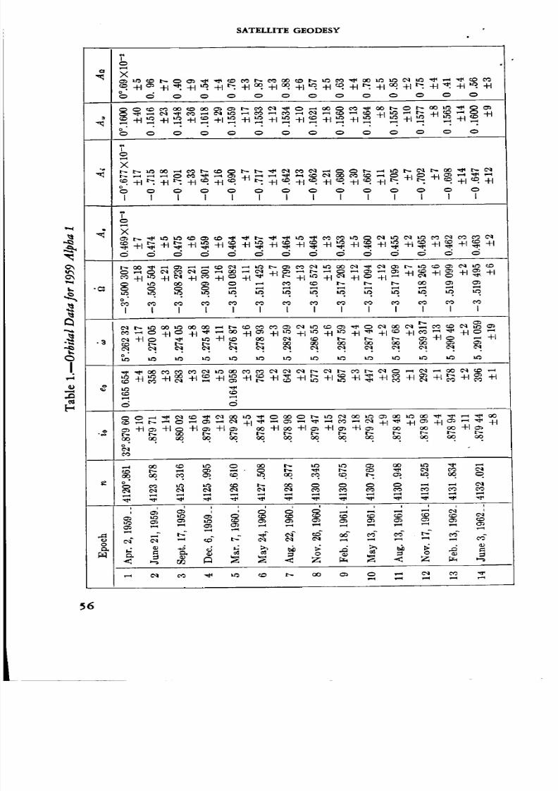
8/7/2019 Significant Achievements in Satellite Geodesy 1958-1964
http://slidepdf.com/reader/full/significant-achievements-in-satellite-geodesy-1958-1964 63/170
SATEI,.[.ITE GEODESY
C_
I
O
4
.3
.3
×
×
I I I I I I L I I I _ I t
T
×
I t I t I i t I I i I I i
56

8/7/2019 Significant Achievements in Satellite Geodesy 1958-1964
http://slidepdf.com/reader/full/significant-achievements-in-satellite-geodesy-1958-1964 64/170
ZONAL HAKMONICS COEFFICIENTS
The earth's gravitational potential is expressed with Legendre polyonomials as
_2
The secular motions of the node and the perigee and the amplitudes
of long-periodic terms with argument _ derived from observations are
compared with those computed from my previous value of J_ (Kozai,
1963),
J_= 1082.48 X 10-e, Ja= -2.562>( 10-6,
J4= - 1.84×10 -6, J6= -0.064X 10-e,
Je = 0.39 × 10 -e, J_ = - 0.470 × 10 -e,
Js--- -0.02×10 -s, Jg= 0.117×10 -6.
(9)
Of course we must include luni-solar secular terms and a J_' term,
which can be computed with an approximate value of J2 to compute
secular motions. Therefore, each secular motion and amplitude pro-
vides us with (O-C), which will make it possible to improve values of J,.
3. DATA
(a) 1959 Alpha 1--Table 1 lists fourteen sets of data for tMs satellite,
and table 2 gives (O-C)'s referred to my previous values for J,.
The standard deviations for the daily secular motions _ and _ given
in table 1 are determined from observations; those in table 2 are com-
puted by adding uncertainties which come from those in e0 and i0.
Weighted mean values for the fourteen sets are given at the bottom of the
table. As can be seen, the scattering of (O-C)'s is much larger than that
expected from the standard deviations assigned to the observed values.
However, the standard deviations assigned to the mean values in table 2
should be more reliable, and will be used in the determinations of J,.
(b) 1959 Eta--Ten sets of data are given in tables 3 and 4 for this
Vanguard satellite. However, its orbital elements are not essentially
different from those of 1959 al and the mean values of (O-C) in table 4
are almost identical with those in table 2, as expected. For the two Van-
guard satellites (O-C) in _2and A_ are significantly large.
(c) 1960 Iota 2---Since the eccentricity is very small for this rocket of
Echo I, the formulas (2) are used in the reduction. Since &_- _ are verysmall for this satellite, it is necessary to take spee_,ial care to compute terms
with arguments 2(_+_--9_) and 2(_+g-_) in the luni-solar per-turbations.
Five sets of data are given in tables 5 and 6. For this satellite the
scattering of (O-C) for secular motions is very large. The large scatter-
57

8/7/2019 Significant Achievements in Satellite Geodesy 1958-1964
http://slidepdf.com/reader/full/significant-achievements-in-satellite-geodesy-1958-1964 65/170
SATELLITE GEODESY
Table 2.--(0-C) Re]erred to Kozai's Previous Constants.[or 1959 Alpha I
_×10 6 _X10 _ A,X10 e A_×10_ Ao×10 4 AuX10 4'
1 ...... 19 ° + 17 °
2 ...... 0+8
3 ...... 3__+8
4 ...... --15 +11
5 ...... 3+6
6 ...... --3+4
7 ...... 6+3
8 ...... --5+_7
9 ...... ! 1+5
10 ..... --4 +_ 3
11 ..... 0+3
12 ..... 13 _ 3
13 ..... 3+3
14 ..... 9___2
Mean__ 4_+2
--31 °± 18°
49 -+23
--23 -+23
--22 -+21
--42 -+13
--33 _+I0
3 _+14
--27 _+17
--24 _+16
-8 _+ 15
-4_+8
--33 _+ 7
--46 _+14
--48 _+ 8
-26 _+ 6
12_+7
17_+5
18_+6
2_+6
7+4
0_+4
7_+5
7_+3
-4_+5
3_+2
-2_+2
8+3
5+3
6-+2
4___2
13° +_17°
--26 +_18
-13 +_33
41 -+16
--3_+7
--31 _+14
44 _+13
24 +_21
6 -+30
18 _+11
-20 _+ 7
-17 +__ 7-13 -+ 14
38 -+ 12
--2+_8
90 ° -+ 40 °
2 -+23
33 -+36
102 -+29
41 ±17
12 _+12
12 _+10
98 +_18
37 _+13
40_+8
31 _+I0
51_+840 _+14
75+_9
42+_8
--9°-+5°
19 _+7
--37 _+9
--23 -+4
--I +_3
I0 -+3
Ii +_6
--20 -+5
--14 -+4
1 _+5
8 -+2
--2 +_4--36 -+4
--21 -+3
-5 -+5
ing for & may be partly due to the fact that the radiation pressure effects
in the argument of perigee are too large to handle accurately. Also, I
suspect that the anomalistic mean motion cannot be determined with
sufficient accuracy for a satellite of such small eccentricity. This might
be one reason why we have large discrepancies in the secular motions of
the node.
ttowever, (O-C)'s in 3, _ and A, are still significant.
(d) 1961 Nu--For this satellite precisely reduced Baker-Nunn observa-
tions are not available and observations must be used that are not pre-
cisely reduced, ttowever, since the satellite is close to the earth and the
inclination is the smallest used in this paper, the node and the perigee
move rapidly and the relative accuracies in the determination of thesecular motions are fair.
Four sets of data are given in tables 7 and 8, which show a wide scatter
in the values of (O-C) in A, and A_. The residuals in the two secular
motions take large values. This satellite was not used in the earlier
determination of Jn; at that time the smallest inclination was 32°.9, for
1959 al.
(e) 1961 Omicron--There are two separate satellites for 1961 o. tIow-
ever, since they have almost identical orbital elements, they are treated
as one satellite here. The eccentricity is very small. Since the inclina-
tion is rather close to the critical inclination, the argument of perigee
moves very slowly. Therefore, one set of observations must cover more
than 500 days. However, as the mean motion changes rather rapidly due
to air drag, I have used one set of 400-day observations.
58

8/7/2019 Significant Achievements in Satellite Geodesy 1958-1964
http://slidepdf.com/reader/full/significant-achievements-in-satellite-geodesy-1958-1964 66/170
• ZONAL HARMONICS COEFFICIENTS
I.
...,,
I-..
"3
,o
+i . _I-. -'H . . • -_L ....
X
_ +J r":. -H r':. "_ r':- +[ _ +t r':. -H _. +t r':- _. "_ _. +t
i l I l I l I I ] I
7
×
I _ _ m _ I m _ m m
I I I t I i i I
o" _
_ oooO oO
i i , _ i, i , .2' ' ' ' '
_ _ _ _ _
_9

8/7/2019 Significant Achievements in Satellite Geodesy 1958-1964
http://slidepdf.com/reader/full/significant-achievements-in-satellite-geodesy-1958-1964 67/170
×
_ ×
T
60
SATELLITE GEODESY
I ilIT_ T
I I I I I
I I I I _ I "_
I I I I t '_, I I I I!
T
×
×
I I I I
T
×
I I _ I I

8/7/2019 Significant Achievements in Satellite Geodesy 1958-1964
http://slidepdf.com/reader/full/significant-achievements-in-satellite-geodesy-1958-1964 68/170
e_
G_
v
I
×
4
x
&
ZONAL HARMONICS COEI_ICIENTS
liter t
o
iLiititlll i
,,_ ,_
.3
T
x
T
x
I I I I
T
×
__
oo _H ._ _Hr.- .H ,.._.Hc_ L_
I I I 1
oO 00 O0
i i i t
61

8/7/2019 Significant Achievements in Satellite Geodesy 1958-1964
http://slidepdf.com/reader/full/significant-achievements-in-satellite-geodesy-1958-1964 69/170
SATELLITE GEODESY
For this satellite, the mean height is rather low, about 900 kin, and
the inclination is high. Therefore, the object is rather difficult to observ_
from the Baker-Nunn stations due to visibility conditions, and there are
many gaps in the observations, periods for which accurate orbital ele-
ments are not available. As the Baker-Nunn stations are between +35 °and -35 ° in latitude, the inclination of this satellite is poorly determined
although the Iongitude of the node can be well determined. This situa-
tion is contrary to that of Vanguard satellites.
Table 8.--(O-C) ]or 1960 Nu
1 .......
2 .... ...
3 . .. .. .. ..
4 .... .... .
Mean _
6 X 10 3
-- 59 ° ± 15 °
--74 ± 10-51 ± 15
--10 ±22
--48 ±20
tl X 10 6
211°+30 °
90 ± 2071 ±80
11l _+45
131 ±40
A,X106
-17± 3
1-14± 3-17± 3
11± 8
-9 ± 14
AIX105 A_0X104
-173°_+44 ° -450_+20 °
-140 ±30 -50 4-_40-105 ±35 --25 ±34
--20 ±24 64 ±61
-110 ±70 --14 ±50
AuX10 _
17 ° ± 5 °
16±621 +11
0 ±12
14 ± 10
The secular motion of the node is determined quite accurately, as we
can see in table 9. However, we cannot compute theoretical values of
the secular motions so accurately as the observed ones, because of uncer-
tainties in the inclination. Therefore, the standard deviations in (O-C)of _'_in table 10 are large. But (O-C)'s in _'_themselves are quite large,
as we can see in table 10. In the previous determination of J,, accurate
orbital elements from Baker-Nunn observations were not available.
The value of (O-C) in 9. for the epoch 4 is quite different from the
others, "rod I suspect this scattering is due to some accidental errors in
i0 for the epoch 4, and give small weight to this value in taking the mean.
For this satellite the radiation pressure effect in the argument of perigee
is too large for my program to compute it with enough accuracy. This is
also true for other satellites of small eccentricity.
(f) 1961 Alpha Delta 1--This satellite has a polar orbit. However,
as the mean height is quite high, we can determine the orbit very accu-
rately from Baker-Nunn observations.
This satellite, and the three listed in tables 13-17, which were launched
in 1962, were not used in my previous determination.
The first set of data is determined from 300-day observations, and the
second set is from 400-day observations, which cover one revolution of
argument of perigee.To compute the solar-perturbations there arise three small divisors,
namely, 2(he-&), 2(&-9+ne) , and 2(ne-2¢5-_).
TabIes 11 and 12 show that the eccentricity is very small and that
(C-C) in _ is very significant.
62

8/7/2019 Significant Achievements in Satellite Geodesy 1958-1964
http://slidepdf.com/reader/full/significant-achievements-in-satellite-geodesy-1958-1964 70/170
ZONAL HARMONICS COEFFICIENTS
o¢b "_"
G_
o
I.
t_
o
x
?O
x
• . 0
I I I
?
X
Cq @4 ¢q
i I ! I
I I I t
g g od o d
¢bO
O_
,?o
0
._= -H-H-H +1 -H
"_ +1 +1 -H +1 t 4-1
X.. _o_""_ I
1 t
+1 +1 4-1 4-1 -H
x _
o4-1 +l 4-t +1 -H
I 1 I I I
+l +i +1+l +_
I
illl_lll ii,ii i
63

8/7/2019 Significant Achievements in Satellite Geodesy 1958-1964
http://slidepdf.com/reader/full/significant-achievements-in-satellite-geodesy-1958-1964 71/170
I.
64
't ?0
X X
,_ +1_, 4-1I
?o
4_ x,-'_ t-,, _'q O0
_, ,=,
? ?
_x x
I t
+1 _ +1
00 00
d
SATELLITE GEODESY
+1
X ._ ,,_ oO
+1 +1 +1
+1 +1 +1
x _-3 L I
I
I i ,
._ o. o. o
o o
_ +ls 7L.4 ?L
o o
"t0
X
I i I
?
00 oO 00
%
+__ +1_ +1
c5

8/7/2019 Significant Achievements in Satellite Geodesy 1958-1964
http://slidepdf.com/reader/full/significant-achievements-in-satellite-geodesy-1958-1964 72/170
"r
ZONAL HARMONICS COEFFICIENTS
+14"1+1 -H
-4-14-1+1 +1
X _ ,,_ ,_
I I t I
X -H -H -H 44
X 4-1 -I-I -'t-I +1
+I+I-H -t-I
1 I I I
'-I-I -H -H -,H
) i i i
_o
I.
<
<
t
X
X
_-H_,-H. H
I 1 I
'i'oX
oO
I I I
Ib,-
,-, ,.,
65

8/7/2019 Significant Achievements in Satellite Geodesy 1958-1964
http://slidepdf.com/reader/full/significant-achievements-in-satellite-geodesy-1958-1964 73/170
66
SATELLITE GEODESY
+1 +[ +t +1
+L +l +1 +1
I 1 I I
11
+1 +1 +1 +1
_ +1 +1 +t +t
_ i i i i
i i i i
i i i i
i i I ii i i Ii i i i1 i i ii i i ii i i ii i I i
i i i ._
,-.,' ' ' N
v
I.p..
_+1 +1
X
$ +l
x X
+1
I
0,1
7 +1
x.-, .,, X I
,_ +_
+1
r_ +1•_ ¢,1
• _ _
I ×4
• 3 _,i_ _
_,1 +1
_ x'_ ":3
0 .
N c
+1
iIi
iii
i
i
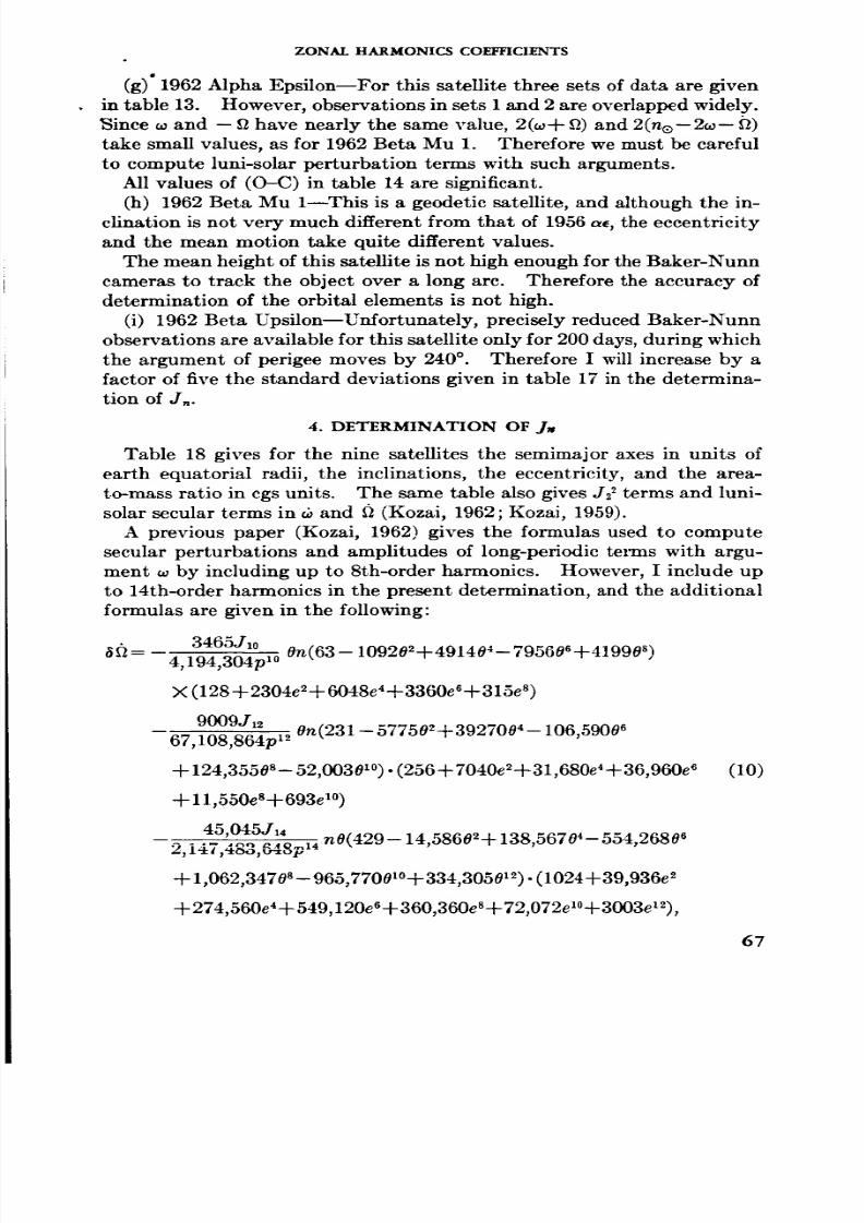
8/7/2019 Significant Achievements in Satellite Geodesy 1958-1964
http://slidepdf.com/reader/full/significant-achievements-in-satellite-geodesy-1958-1964 74/170
ZONAL HARMONICS COEFFICIENTS
(g)" 1962 Alpha Epsilon--For this satellite three sets of data are given
in table 13. However, observations in sets 1 and 2 are overlapped widely.
Since _ and - _2 have nearly the same value, 2(_+ _) and 2(no-2_-- _2)
take small values, as for 1962 Beta Mu 1. Therefore we must be careful
to compute luni-solar perturbation terms with such arguments.All values of (O-C) in table 14 are significant.
(h) 1962 Beta Mu 1--This is a geodetic satellite, and although the in-
clination is not very much different from that of 1956 a_, the eccentricity
and the mean motion take quite different values.
The mean height of this satellite is not high enough for the Baker-Nunn
cameras to track the object over a long arc. Therefore the accuracy of
determination of the orbital elements is not high.
(i) 1962 Beta Upsilon--Unfortunately, precisely reduced Baker-Nunn
observations are available for this satellite only for 200 days, during which
the argument of perigee moves by 240*. Therefore I will increase by a
factor of five the standard deviations given in table 17 in the determina-
tion of jn.
4. DETERMINATION OF Js
Table 18 gives for the nine satellites the semimajor axes in units of
earth equatorial radii, the inclinations, the eccentricity, and the area-
to-mass ratio in cgs units. The same table also gives J2 _ terms and luni-
solar secular terms in _ and _ (Kozai, 1962; Kozai, 1959).
A previous paper (Kozai, 1962) gives the formulas used to compute
secular perturbations and amplitudes of long-periodic tel_as with argu-
ment w by including up to 8th-order harmonics. However, I include up
to 14th-order harmonics in the present determination, and the additional
formulas are given in the following:
_= 3465J10 0n(63-109202_491404- 79560e _-41990s)4,194,304p 1°
X (128-k2304e2_- 6048e4_3360eeW315e s)
9009J12
67,108,864pl 2 0n(231 - 577502_3927004-106,59006
+ 124,3558 s- 52,00301°) • (256_- 7040e2-_31,680e4+36,960e 6 (10)
11,550eST 693e 1°)
45,045J14
.... _Q 14n0(429-14,5860_-F138,56704-554,2680 ez, 147,4_o,,-_p
_- 1,062,3470 s- 965,7700_°-_334,3050_2) • (1024_-39,936e 2
-_274,560e4_- 549,120ee_-360,360eST72,072el°_-3003e12),
67

8/7/2019 Significant Achievements in Satellite Geodesy 1958-1964
http://slidepdf.com/reader/full/significant-achievements-in-satellite-geodesy-1958-1964 75/170
SATELLITE GEODESY
O [1111 Ill
68
.a
x
o .........
I I il_
X
II
?
×
II
IllllllllI lillllliii

8/7/2019 Significant Achievements in Satellite Geodesy 1958-1964
http://slidepdf.com/reader/full/significant-achievements-in-satellite-geodesy-1958-1964 76/170
ZONAL HARMONICS COEFFICH_N'TS
3465J,o nf63_346502+30,O3004_90,ogooe+109,395088,388,608plo ,
- 46,1890'°)- (128+ 1152e2+2016e4+840ee+63e 8)
9009J12 n(231 --18,01803+225,22504-1,021,02006268,435,456p 12
+2,078,50508-1,939,93801°+676,0390'2) • (1024+39,936e 2
+ 274,560e4+549,120e6+360,360es+72,072el°+3003e '_) (11)
45,045J14 n(429_ 45,0450_+ 765,76504_ 4,849,8450e
-- 4,294,967,296p14
+ 14,549,53508- 22,309,2870,0+ 16,900,9750 TM- 5,014,5750'4)
X (1024 + 19,968e 2+ 91,520e 4+ 137,280e 6+ 72,072e 8
+ 12,012e'°+429e12),6
5e= --sin i (1--502)-'(1--e2)_ C_AjB_ sin o_, (12)
y--4
_{= -- e0 _e/{ sin i (1 -- e 2) }, (13)6
_fi=e0 sin -1 i (1--502) -' _ C_{ -sin 2 i.Dj
+(9-50')(1--502)-'Aj}Bj cos _,, (14)
6
5o_= --O$_--sin i.e-'. (1--503) -' _ CjA_Ej cos _o, (15)
69
where
0 = cos i
105J9C,=
65,536J2p 7
1155JuC_=
4,194,304J2p 9
Ca = 3003J,s
67,108,864J_p n
A 4= 7-- 30802-t-200204- 4004_ + 2431
A 5= 21 -- 136502-{-13,65004- 46,4100e+ 62,98508- 29,3930 '0
A 6= 33-- 297002+42,07504- 213,1800e+479,65508- 490,31401°+ 185,7250 TM

8/7/2019 Significant Achievements in Satellite Geodesy 1958-1964
http://slidepdf.com/reader/full/significant-achievements-in-satellite-geodesy-1958-1964 77/170
SATELLITE GEODESY
B4 = 64 -_-336e 2_- 280e 4-_-35e 6
B_ = 128+ 1152e2-_ 2016e4-_840e6-_-63e s
B8 = 512 -_-7040e2 _- 21,120e4-_ 18,480e6 -_-4620eS q- 23 le 1°
D4 = 88(7- 9102+27304- 22108)
D5 = 130(21- 42002+214204- 387608+ 22610 s)
D8 = 60(99 - 280502+ 21,31804- 63,95408+81,7190 s- 37,1450 '°)
E 4= 64 +17 76e2+ 476 0e4-t- 2485eS-_- 210e8
E5 = 128-b5504e2q-26,208e4+30,072eS+ 8,967eS-_- 504e'n
E8 = 512-t-31,360e2q- 232,320e4-_-467,280eS-_-300,300eS+ 57,982e 1°+ 2310e 1"_
(16)
(a) Even harmonics--Table 18 gives equations of condition to deter-
mine values of J2 through J,4. There are 18 equations with 7 unknowns.
The equations can be solved by assigning to each a weight reciprocally
proportional to the standard deviation. Actually, each equation is
divided by its standard deviation, and then normal equations are con-
structed. Before solving the equations, note that 2;(O-C) 2 is 3882
(= 18X14.7:); that is (O-C) is bigger than the standard deviation by
factor of 14.7. This value comes down to 23 = (18- 6) X 1.42 after solving
J,2, and to 13.4=(18-7)X1.12 after solving J,4, whereas it is 93.5=
(18-5)×2.72 after J,0 is solved. Therefore we can stop either at J12 or
at J,,, although the solution including J14 is, of course, better.
In table 19 residuals based on the solutions up to J,4 and J,2 are given
under headings I and II, respectively, in units of 10-6 degrees. Under
the heading KH, residuals based on King-Hele and Cook's values (1964)
are given; that is,
J2 -- 1802.70X 10 -6, J4 - - 1.40 X 10 -6,
J6 -- 0.37X10 -6, Js = 0.07X10 -_,
J10 = -0.50)10 -8, J12 = 0.31)10 -6. (17)
In the node equations the residuals based on my new determinations
for 1962 3v are larger than the standard deviations. However, since this
datum is not entirely reliable, being based on a single determination cov-
ering an incomplete period of time, this may not be a weak point in this
determination.In the perigee equations of 1961 v and 1962 aE, the residuals are larger
than their standard deviations. This may suggest that we must still
include higher-order terms to express these data.
7O
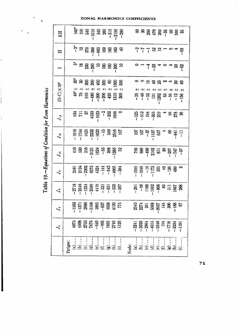
8/7/2019 Significant Achievements in Satellite Geodesy 1958-1964
http://slidepdf.com/reader/full/significant-achievements-in-satellite-geodesy-1958-1964 78/170
_t
I.
×1
i
%
ZONAL HARMONICS COEFFICIENTS
I
I1
t t
+t _ ÷l+l _ +[÷1 ÷1
I
I
17 i
I °
I
.I
It I
F
_ I_ _ _ iI
tli i
lilt
I
•_ ,_f fq t'.- I j ,--_ C,_ ',-'*
IIIII III
Illlt_ll I
illlllll ,
"_ o
71

8/7/2019 Significant Achievements in Satellite Geodesy 1958-1964
http://slidepdf.com/reader/full/significant-achievements-in-satellite-geodesy-1958-1964 79/170
SATELLITE GEODESY
v-4
I "_ I I_ I "_ I"_ I I I"
I IC_ _ I _
• o o
I I_ I I I!
_ _.
Ill_l II
I I I I
I IIIII I
L 71_
I I
7"_7 _7 J II I
I Illl II
o
ii
iio
72

8/7/2019 Significant Achievements in Satellite Geodesy 1958-1964
http://slidepdf.com/reader/full/significant-achievements-in-satellite-geodesy-1958-1964 80/170
ZONAL HARMONICS COEI:FIC/3BNTS
t,-
I
I
I
--H -H -H
I
_o0
II _ _ ©I
I
c0
+I-H ,_-H+.I-H-.H-FI-.I.'I-.I.-I-I-I-.I-.I
I
I I
IIII I I I
8_
I I
iT' _T T I
i I"_1 I1 I I
i ,
i i
, ii ii i
; !i ii i
ii
i!i1
iii
'Z
i i
i ii ii ii i
, ii i
i
73

8/7/2019 Significant Achievements in Satellite Geodesy 1958-1964
http://slidepdf.com/reader/full/significant-achievements-in-satellite-geodesy-1958-1964 81/170
SATELLITE GEODESY
The two sets of solutions derived are the following:
Solution I (in units of 10-7)
dJ2= 1.65, dJ4 -- 1.81, dJ6 = 2.56, dJ8 =-2.50,
+6 +_16 +30 +50
J10 = - 0.54, J,2 = - 3.57, J,4 = 1.79,
+50 -+44 ___63
(18)
Solution II (in units of 10-7)
dJ= = 1.50, dJ4 = 2.03, dJ6 = 2.03,
+_5 __+18 _+31
dJ8 = -1.29, J10 = -1.55, Jl:= -2.94.
+_.34 -+45 -+49
(19)
(b) Odd harmonics--As shown in table 20, we have 32 equations to
determine 6 unknown coefficients of odd harmonics. At first -v(O-C) 2
is 349(=32X3.32). This number comes down to 153(=28>(2.3 '_) after
J9 is solved, and to 42(=27X 1.252) and to 39(=26X 1.23 _-) after J,1 and
J13, respectively, are solved. Therefore, the inclusion of J,3 does not
reduce the residuals too much. Two sets of solutions are derived, one
up to J,l and one up to J13; that is,
Solution I (in units of 10 -7)
dJ3 = 0.31, dJ5 =-1.47, dJ7 = 1.36,
-+20 _ 25 -+39
J9 = - 1.67, Jll = 3.02, J13 = - 1.14,
-+60 -+35 4- 84
Solution II (in units of 10-7)
dJ3 = 0.07, dJ5 =-1.22,
4-11 ___17
dJ7 = 0.93,
+_22
J9 =-0-75, Jll--- 2.96. (20)
-+ 17 -+35
Table 20 gives the residuals based on solutions I and II for each datum.
Residuals in the eccentricities of 1961 v and 1962 /_, in the perigee of
1961 _, and in the nodes of 1962 ae and 1962 fly have much larger values
than the standard errors. This may show that still higher-order har-
monics are significant.
74

8/7/2019 Significant Achievements in Satellite Geodesy 1958-1964
http://slidepdf.com/reader/full/significant-achievements-in-satellite-geodesy-1958-1964 82/170
ZONALARMONICSOEFFICIENTS
In this analysisparallacticermsareneglectedn computingunar• perturbations.However,n theparallacticdisturbingunctionthereis
_; term,
@sin/-sin _(1 5 . (1--5 sins sin ,.,.sin to',-i sm _ i) e)ee'(1 +43-e2) (21)
where _ is obliquity, e is lunar eccentricity, and to' is lunar argument of
perigee. Since to' moves slowly, we must include this term if we treat
observations of high-altitude satellites in the future.
5. RESULTS
The two sets of solutions derived in this paper are the following:
Solution I (units of 10-e)
J2 = 1082.645, Js -- -2.546,
_+6 _+20
J4 = -- 1.649, J5 = -0.210,
-4-16 -4-25
Je = 0.646, J7 -- - 0.333,
_ 30 _+39
Js = - 0.270, J9 = - 0.353,
_ 50 _+60
J,0= -- 0.054, Jn = 0.302,
+50 -+35
Jl_= -0.357, Jl_= --0.114,
+44 +84
J14= 0.179
_+63 (22)
Solution II
J2 = 1082.630, J_ = -2.559,
_+5 _+11
J4 = -!.627_ J5 =-0-185,
+18 _+17
Js -- 0.593, J7 = -0-376,
-+31 _+22
75

8/7/2019 Significant Achievements in Satellite Geodesy 1958-1964
http://slidepdf.com/reader/full/significant-achievements-in-satellite-geodesy-1958-1964 83/170
SATELLITE GEODESY
Js = -0.149, J9 = 0.039,
+ 34 4-17
J10= -0.155, Jli= 0.296,
__.45 ±35
J1_= -0.294
4-49 (23)
A. H. Cook (1964) recently derived values of J_, J4 and Je by using high
satellites only, and his results show remarkable agreement with Solution I.
The flattening of the reference earth ellipsoid based on this value of
J_ is 1/298.252. The theoretical value of J4 for the reference ellipsoid
assumed to be in hydrostatic equilibrium is computed as -2.350× 10⁻⁶ .
The deviation of the geoid computed on the geopotential based on solution
I is expressed as a function of geometric latitude:
h=-_0.8-18.3 sin _-87.8 sin s f_-l19.1 sin s f_-b1042.5 sin 4
-_1191.7 sin 5 f_-5074.2 sin 6 _-3636.7 sin _ _-{-12,668.0 sin 8
-_5230.8 sin 9 _-16,676.3 sin 1° f_-3556.4 sin 11/_-10,913.0 sin TM
-_926.8 sin is _--2791.3 sin1' fl (in meters). (24)
Figure 1 shows the value of h as a function of f_ based on this equation.
The value of geoid height h in the north pole is 13.5 meters, which is the
maximum value, and is -24.1 meters in the south pole.
In tile solutions (22) and (23), the values of J, do not tend to converge
to zero as n increases. However, if n is large enough, J, should take a
very small value. Otherwise the gravity expression, which is derived
by differentiating the potential with respect to the radius, may give a
very great difference of gravities between the equator and the poles and
between the north and south poles.
To determine how strong or weak the solutions (22) and (23) are, thecorrelation coefficients in my determinations are shown in tables 21 and
22. The tables indicate that these solutions are derived from rather
strongly correlated equations of condition. Therefore, in the future we
must use both low and high satellites having the same inclination.
However, to determine the orbital elements of low satellites _ith high
inclinations we need observations from high latitudes. As I mentioned
earlier, I could not assign a large weight to the node equation of 1961o
to determine even-order coefficients, because the inclination could not
be determined with sufficient accuracy. Also, I must mention that I did
not use satellites with inclinations below 28 °, between 50 ° and 67 °, or
between 67 ° and 85 ° in this determination.
76
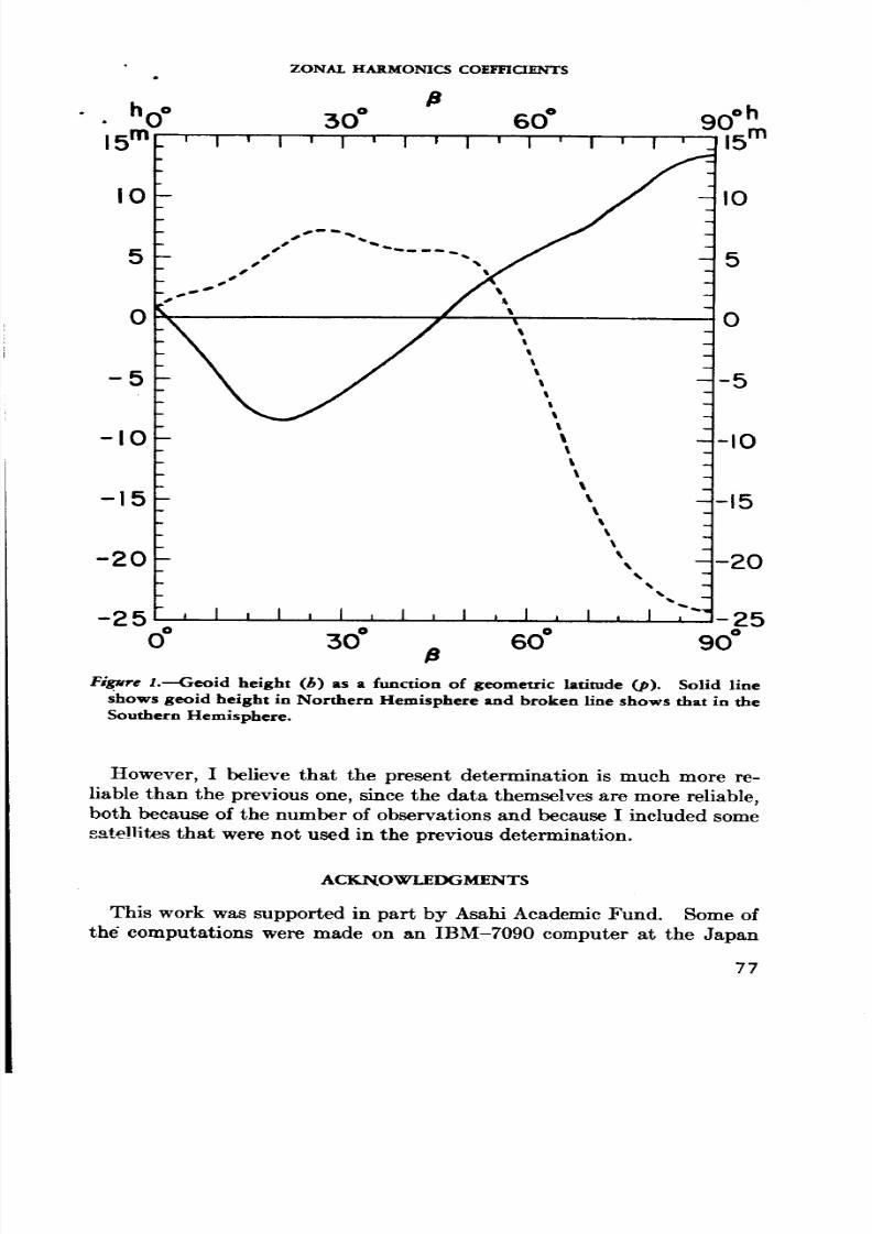
8/7/2019 Significant Achievements in Satellite Geodesy 1958-1964
http://slidepdf.com/reader/full/significant-achievements-in-satellite-geodesy-1958-1964 84/170
ZONAl. HARMONICS COEFFICIENTS
• ho o 30 ° 60 ° 90'h15m ' = ' = , I ' I , I , = ' i , i , _15
I0
5
0
-5
t
-I0
-15
I
I
1
lI
l
I0
5
0
-5
-I0
-15
-20
I
-20%
%.
-25 , J, I, I, J, i, I, i, i , -25
oo 3o° 6o° 9o°
Fibre l.--Geoid height (h) as a function of geometric latitude (p). Solid line
shows geoid height in Northern Hemisphere and broken line shows that in the
Southern Hemisphere.
However, I believe that the present determination is much more re-
liable than the previous one, since the data themselves are more reliable,
both because of the number of observations and because I included some
satellites that were not used in the previous determination.
ACKNOWLEDGMENTS
This work was supported in part by Asahi Academic Fund. Some of
the" computations were made on an IBM-7000 computer at the Japan
77

8/7/2019 Significant Achievements in Satellite Geodesy 1958-1964
http://slidepdf.com/reader/full/significant-achievements-in-satellite-geodesy-1958-1964 85/170
78
?(,,4
e_oS
SATELLITE GEODESY
I I I
i
t I :t
IL
I I , ,iiii
iL*
I t i i
I1
ILII
_8 .... II
_ _ "''lill
Jill
liil
iiii
iI_ll
llllli_lll_llll
,ill,
.... :I
I I I
L
i
i L , ,
r_
i
_ I :11
i,,i
_ .....llli
Illi
_ _ • ,
iilili
tillil(1111
111111
tlilll
:I:1111
% L i
i
i I :
i i
iii
IIII
"IIII
_ _ : , , ,bill
I_LL
llil
I t I
I I :
IL
_N_,'
t_
• . o
I 1 g:,
_ ....t_
_ ,ittl
I'[I,
LIIII
I_lil
'illll
_ _ , , : , ,
IIIII

8/7/2019 Significant Achievements in Satellite Geodesy 1958-1964
http://slidepdf.com/reader/full/significant-achievements-in-satellite-geodesy-1958-1964 86/170
ZONAL HARMONICS £O_'IOENTS
IBM Co., which kindly provided machine time without charge throughthe Computing Center of the University of Tokyo. I am grateful to
Miss Phyllis Stem for her help in the computations.
REFERENCES
CooK, A. H.:
1964. Paper presented at IAU Commission 7 Meeting, Hamburg, August.
KINC_-HELE, D. G., AND COOK, G. E. :
1964. A paper presented at meeting of COSPAR Working Group 1, Florence,
Italy.KOZAI, V. :
1959. Smithsonian Astrophysical Observatory, Special Report No. 22, 7.
1962. Astron. J., 67, 446-461.
1963. The Use of Artificial Satellites for Geodesy, ed. G. Veis, 305-316.
79
8/7/2019 Significant Achievements in Satellite Geodesy 1958-1964
http://slidepdf.com/reader/full/significant-achievements-in-satellite-geodesy-1958-1964 87/170
• _ PAGE BLA_iK NOT FILMED.
Part 3
Derivation oJ the Earth's Gravity Field by
Nonoptical Tracking
Although precision optical tracking has yielded the
most extensive geodetic information to date, electronic
tracking methods are rapidly becoming competitive.
Of the latter methods, the precise measurement of thefrequencies received from stable oscillators in the
satellite has been particularly fruitful.
A section of a recent report by Dr. Robert R. Newton
of the Applied Physics Laboratory, one of the group
which has exploited this technique most successfully,
provides an explanation of the basic technique. This
is followed by a report of the analysis of some of the
Doppler data and data from Syncom 2.

8/7/2019 Significant Achievements in Satellite Geodesy 1958-1964
http://slidepdf.com/reader/full/significant-achievements-in-satellite-geodesy-1958-1964 88/170
The following is excerpted from a paper presented by Robert
R. Newton at the European Symposium on Satellite Geodesy,Paris, December 1964.
Measurements oJ the Doppler Shift in Satellite
Transmissions and Their Use m Geometrical
Geodesy
ROBERT R.NEWTON
Applied Physics Laboratory
Johns Hopkins University
1. CHARACTERISTICS OF EXISTING DOPPLER MEASURING EQUIPMENT
HE APPLIED PHYSICS LABORATORY exercises technical direction on
behalf of the Department of the Navy of a network of doppler
tracking stations that is called the TRANET System. This system has
been in operation for approximately five years and currently contains
twelve stations with another expected to be added in 1965. Many other
sites have been occupied at various times. The Department of the Navy
maintains this tracking system and supports geodetic analysis of the data
obtained from it as a part of the national geodetic satellite program.*
Up to the present, the data from this system have been used almost
entirely in studying dynamics of satellites and in deriving models of the
earth's gravity field from these dynamic studies.
The method of operation of the existing doppler stations is described
in Ref. 1. Briefly summarized, a station makes a measurement of doppler
frequency every 2 or 4 seconds and thus typically obtains several hundred
data points during each pass of a satellite.
In these measurements the effects of radio noise and of instrumental
contributions to error are virtually negligible. The dominant errors in
the raw data arise from refraction both in the ionosphere and in the
troposphere.Of these two sourccs of refraction ionospheric refraction is by far the
*The station in Antarctica, if it is established, willbe supported by the National
Science Foundation, and therefore is not strictly speaking a part of the TRANETSystem. However, data from it will be available for analysis so that it can be con-sidered together with the other stations for the purposes of this paper.
83

8/7/2019 Significant Achievements in Satellite Geodesy 1958-1964
http://slidepdf.com/reader/full/significant-achievements-in-satellite-geodesy-1958-1964 89/170
I SATELLITE GEODESY
biggest problem. If no correction were made for refraction in the iono- •
sphere at a transmitted frequency of 162 mh, for example, satellite posi-
tions derived from the doppler measurements could easily be in error by
as much as a kilometer. Fortunately, the refractivity in the ionosphere
depends upon the frequency and to first approximation varies inversely
with the square of the frequency. This fact is the reason for using two
or more transmitted frequencies (see Refs. 1 and 2) which are both con-
trolled from the same oscillator and which are hence always coherent. By
measuring the apparent doppler shift at each of two coherent frequencies,
it is possible to calculate the effects of ionospheric refraction and therefore
to eliminate refraction, on the assumption that the refractivity does
indeed vary with the square of the frequency. Since this law does not
hold exactly, there is some residual refraction arising from neglectedeffects. At middle and high latitudes we believe that the residual effects
amount to the equivalent of a few meters or less in satellite position.
However, there is some indication that at low latitudes and under some
circumstances the residual effect may amount to 100 meters or more.
Fortunately, position errors from residual refraction have a tendency to
average out when many satellite passes are used.
Depending upon the level of accuracy desired, the uncorrected iono-
spheric refraction may still be unacceptable. There are three ways of
reducing the effect of refraction still further. One is by the use of a third
frequency which will be provided on GEOS A (Ref. 3). A second method
which shows promise involves a calculation of the higher order refraction
effects based upon a model of the ionosphere, combined with the measured
refraction effect obtained from two frequencies. There is considerable
hope that the higher order refraction can be calculated in this way to an
accuracy of about 10% of the high order effects. The third way is to
use higher frequencies such as the 972 mh beacon provided on GEOS A.
Tropospheric refraction effects can produce the equivalent of about
50 meters in satellite position if no correction is made. Tropospheric
refraction does not depend appreciably upon frequency and therefore
cannot be removed by the techniques that are successful with the iono-
sphere. Up to the present time the only way that we have found to
correct for tropospheric refraction (Ref. 4) is to calculate this refraction
using a model of the troposphere combined with suitable meteorological
observations made at the time of each pass. This correction has been
quite successful except when a weather front is near a station at the time
of a pass. If high accuracy is desired it is necessary to eliminate anydata obtained when a weather front is within about 30 km of a station.
As we have already said, the stations that make up the TRANET Sys-
tem supply several hundred data points during each pass. This volume
of data is necessary for many research purposes such as research into the
84

8/7/2019 Significant Achievements in Satellite Geodesy 1958-1964
http://slidepdf.com/reader/full/significant-achievements-in-satellite-geodesy-1958-1964 90/170
m 4
DOPPLER SHIFT IN SATELLITE TRANSMISSIONS
effects of tropospheric refraction which were just discussed. However,
if the presently used methods for eliminating refraction are considered
by an observer to be sufficiently accurate, and if his principal interest is
in using the doppler data for geometric purposes, he can work with muchsimpler receiving equipment which provides a much smaller volume ofdata.
This simplified equipment is now under development at the Applied
Physics Laboratory.
REFERENCES
1. WEIFFENBACH, G. C. : Measurement of the Doppler Shift of Radio Transmissions
From Satellites. Proc. of the IRE, v. 48, no. 4, pp. 750-754, April 1960.
2. GUIER, W. H. ; AND G. C. WEIFFENBACH: h Satellite Doppler Navigation System.
Proc. of the IRE, v. 48, no. 4, pp. 507-516, April 1960.
3. NEWTON, R. R.: Characteristics of the GEOS A Spacecraft. Fresented at the
Symposium on the Establishment of a European Geodetic Network by Artii_cial
Satellites, Paris, France, 14-16 December 1964.
4. HOPFIELD, H. S. : The Effect of Tropospheric Refraction on the Doppler Shift of
a Satellite Signal. J. Geophys. Res., v. 68, no. 18, September 15, 1963.
85

8/7/2019 Significant Achievements in Satellite Geodesy 1958-1964
http://slidepdf.com/reader/full/significant-achievements-in-satellite-geodesy-1958-1964 91/170
I_R_tgG PJ_GllB_K _ R'tW,_,
The fallowing paper was originally published in Nature,
vol. 200, No. 4902, October 12, 1963, pp. 124-125.
N66 37352Determination o/the Non-Zonal Harmonics o]" -
the Geopotential From Satellite Doppler Data
W. H. GumR
Applied Physics Laboratory
Johns Hopkins University
A ]LEAST SQUARES DETERMINATION" of values for the coefficients,C,_, S_, of the non-zonal harmonics of the geopotential:
P: (sin }( ._ m_0 r" [C_ cos mX.-{-S_ sin ink] (1)
has been made through n =m =4 using Doppler data from the three
Satellites 1961 ol, 1961 a_ql, and 1962 3#1. In equation (1):
r -- geocentric radius from the Earth's centre of gravity; _ =geocentric
latitude; ), =geocentric longitude from Greenwich meridian,
and P,_(z) are the associated Legendre polynomials:
m d,a
P'2(z) = (1 -z2) -_ _-_ P_(z) (2)
The values of C_ and S_ were constrained to be identically zero in thedetermination.
Table 1 presents a brief summary of the Doppler data which were
chosen for the determination. The data were chosen as being the best
available from the point of view of: (1) quality with respect to noise-
level, timing errors, presence of ionospheric refraction errors, and stability
of the satellites' transmitted frequencies; (2) uniform distribution of sta-
tion locations over the Earth's surface with particular care taken to avoid
an overweight of data from stations located within the continental
TT_:._m_e_,S_o¢,_;_.._._) uniform coverage of the satellite orbit by the data with
respect to the angle between the ascending node and the Greenwich
meridian.
The principal ionospheric refraction contribution was removed by
coherently combining two frequencies received simultaneously from the
87

8/7/2019 Significant Achievements in Satellite Geodesy 1958-1964
http://slidepdf.com/reader/full/significant-achievements-in-satellite-geodesy-1958-1964 92/170
SATELLITE GEODESY
satellite in the Doppler receiving equipment1'L To ensure further mini-
mum refraction errors, data were considered only if the maximum eleva.
tion of the pass was less than 83 ° and greater than 20 °. Finally, data
points which corresponded to instantaneous elevations below 13 ° were
deleted, and the remaining data points corrected for tropospheric refrac-tion 3. A typical noise-level for that data finally chosen was roughly 5
parts in 10 l° of the transmitted frequency. Timing errors were judged
to be below 0.003 sec (3-sigma value).
The data which survived the foregoing criteria were then grouped by
days, one group containing all passes for a given satellite which occurred
between two successive midnights (G.M.T.). After grouping, only those
were selected which contained ten or more high-quality sets of data from
at least five separate stations with at least three being outside the conti-
nental United States. From Table 1 it can be seen that the fewest groups
of data for any one satellite occurred for Satellite 1961 a_l. This is due
to the low inclination of the satellite precluding reception of data from
high-latitude stations. While considerably more groups of data satis-
fying the foregoing criteria were available for the other two satellites, the
total number of groups chosen for each satellite was limited to being
roughly equal to avoid overweighting the data corresponding to a particu-
lar inclination. In the final choice of groups care was taken to ensure a
reasonably even distribution of angles between the ascending node andthe Greenwich meridian at the time of the first pass in each group. In
addition, groups for two different satellites occurring on the same day
were avoided to increase the a priori probability that the effects of unde-
tected station instrumentation errors and refraction errors were random.
Having made the final choice of groups, a least-squares determination
of a satellite orbit for each group was made, resulting in no computed arc
of the satellite motion lasting more than 24 h. Orbit parameters span-
ning data over such short time-intervals were chosen because: (1) the
satellite trajectory could be integrated numerically with negligible error
and made unnecessary the very tedious task of solving the perturbed
equations of motion to high orders; (2) unknown fluctuations in atmos-
pheric drag and errors in the values for the zonal harmonic coefficients
introduce negligible errors.
The computer programme used to determine the orbits 4 includes the
Sun and Moon forces, although they should introduce negligible errors
for these short data spans. The resulting differences between the
Doppler data points and the corresponding computed values for the
Doppler shift (based on fixed initial values for the harmonic coefficients
of the geopotential) were used as the final data for the least-squares
determination of the differential changes in the values of the non-zonal
harmonic coefficients.
88

8/7/2019 Significant Achievements in Satellite Geodesy 1958-1964
http://slidepdf.com/reader/full/significant-achievements-in-satellite-geodesy-1958-1964 93/170
• NON-ZONAL HARMONICS OF THE GEOPOTENTIAL
,-4
C_ _'_ _
O
_o Io i
z !
.__'__
6
.o
e-.
°o _
XXXXXXXX
..... .°o
I t t I
g_ XXXXXXXX
_....°..
I I
I_,'_1 _'_ _,'a _"_ -_ _ '_ _ '_
89

8/7/2019 Significant Achievements in Satellite Geodesy 1958-1964
http://slidepdf.com/reader/full/significant-achievements-in-satellite-geodesy-1958-1964 94/170
SATELLITE GEODESY
Very briefly, the least-squares procedure used for determining the non-
zonal harmonic coefficients was the following. The differences between
the theoretical and experimental values for the Doppler shift were as-
sumed to arise wholly from errors in the locations of the tracking stations
and values for the non-zonM harmonic coefficients. It was further
assumed that because of these errors there existed errors in the orbit
parameters associated with each group of data. Perturbation equations
were then derived to express these residuals as a function of differential
changes in the three co-ordinates of each tracking station represented in
the totality of data, differential changes in each of the six orbit param-
eters for each group of data, and differential changes in the values of
the C_ and S_ of equation (1). A special IBM 7094 computer pro-
gramme was designed and coded in which the differential values of thestation positions and orbit parameters are continually adjusted to yield
an extremum of the mean-square data residuals with respect to these
parameters (irrespective of whether the resulting values are reasonable)
for any given values for the differential harmonic coefficients. Conse-
quently, at any point in the computing process, changes in the values of
the differential station and orbit parameters can produce negligible
reduction in the mean-square data residuals. In this way the station
co-ordinates and orbit parameters are effectively eliminated from the
least-squares determination of the harmonic coefficients. The pro-
gramme is then iterated until stable values for the differential non-zonal
harmonic coefficients are obtained.
Table 2 presents the results of the determination using the data sum-
marized in Table 1. Without new data at a different inclination, it is
very difficult to estimate the true error in these values; and no attempt
has been made to ascribe a realistic error to each coefficient. The fact
that the station parameters were effectively eliminated from the deter-
mination ensures that the principal error in the resulting values for thecoefficients arises from correlated errors in the experimental data and not
from erroneous values for the station locations. Consequently, the
efficacy of this method depends principally on there being sufficient ex-
perimental data of sufficient accuracy that the build-up of computer error
combined with experimental errors does not destroy the sensitivity of
the data residuals to the harmonic coefficients once the station and orbit
differential parameters are eliminated. Several numerical experiments
were performed with the amount of data intentionally reduced to the
point where a realistic solution would not be expected. The objective of
the experiments was to obtain criteria for the number of harmonic coeffi-
cients which could be evaluated with the data available. As expected,
these experiments indicated that if stable values for the coefficients were
produced with successive iterations, and if their resulting values did not
90

8/7/2019 Significant Achievements in Satellite Geodesy 1958-1964
http://slidepdf.com/reader/full/significant-achievements-in-satellite-geodesy-1958-1964 95/170
° NON-ZONAL HARMONICS OF THE GEOPOTENTIAL
• change markedly with changes in the relative weighting of the data
residuals, the final values should be trustworthy.
Recognizing that the Tesseral harmonic, n=2, re=l, should have
negligibly small coefficients, a final check on the validity of the values in
Table 2 was made by performing a new determination with C_ and S_
added to those coefficients listed in Table 2. The resulting values for
those coefficients in Table 2 were not materially altered and the values
for the new coefficients were found to be:
(3)
The fact that they are negligibly small (compared with the values in
Table 2 for m= 1) lends considerable credence to the values given in
Table 2.
A comparison between the values given in Table 2 and the present
literature 5-8 indicates agreement of roughly the same character as the
agreement between any two previously published sets of values. Conse-
quently, such comparisons add little additional information on the
accuracy of the values presented in Table 2.Clearly the overall effort involved in obtaining these results was very
large, and it is impossible to acknowledge all the people who made valu-
able contributions. However, I wish to acknowledge especially the
contributions of R. R. Newton and S. Yionoulis for their aid in develop-
ing the satellite perturbation equations; G. Worsley, G. C. Weiffenbach,
P. E. P. White, and their colleagues in connexion with obtaining the
experimental Doppler data; and H. D. Black, C. Weisert, R. Henderson,
and their colleagues for their help in coding and running the complex
computer programmes involved.
This work was supported by the Department of the Navy, Bureau of
Weapons, under contract NOw 62-0604-c.
1 GUIER, W. H.; AND WEIFFENBACH, G. C.: Proc. Inst. Rad. Eng., 48, No. 4507
(196o).
2 GVIER, W. H.: (L), Proc. Inst. Rad. Eng., 49, No. 11, 1680 (1961).
a HOPFIELD, H. S.: J. Geophys. Res. (in the press).
Applied Physics Laboratory, The Johns Hopkins University, Rep. TG-401.
KozAI, Y.: Smithsonian Astrophysical Obs., Res. Space Sci., Spec. Rep. No. 72,
August, i961.
6 NEWTON, R. R.: Proc. Third Intern. Space Sci. Symp., Washington, D.C., April,
1962 (in the press).
KAVLA, W. M.: J. Geophys. Res., 68, 473 (1963).
8 IZS._K, I.: Nature, 199, 137 (1963) and private communication.
9l

8/7/2019 Significant Achievements in Satellite Geodesy 1958-1964
http://slidepdf.com/reader/full/significant-achievements-in-satellite-geodesy-1958-1964 96/170
Most gead_ic data have been derived from comparatixelynsar-Earth satellites. However, some of the terms in the
Earth's gravity field are masked for these satellites by various
diurnal effects. Conversely, a satellite in a 2_-hour orbit is
particularly sensitive to these terms because it is constantly
affec_d by the same perturbations. Because of its high
alLitudes, a _-hour satellite is di_cul2 to track optically and
the Minitrack irderferometer does not have the angular accu-
racy needed, To overcome this problem, an electronic trans-
ponder has been developed which provides a measure of both
the diatanee to the aaI_ite and its radial velocity. This tahoeand range-rate system was used on the Syncom satellite.
The geade_ic analysis of thetrackingesu_ is reported in the
following paper which was originally published in the Journal
of Geophysical Research, vol. 70, no. 6, 1965, pp. 1566-1568.
A Determination oJ Earth Equatorial Ellip-
ticity From Seven Months o/Syncom 2
Longitude DriJt
C. A. WAOI,,_R
Goddard Space Flight Center, NA£A
Tby 24-HOVR Syncom 2 satellite has been under periodic observationrange and range rate radar and Minitrack Radio Interferometer
stations since mid-1963 (Wagner, 1964b). Seven months of longitude
drift in the vicinity of two momentarily stationary configurations were
analyzed for sensitivity to hypothetical longitude components of the
earth's gravity field which would be in "resonance" on such a satellite
(Blitzer et al., 1962; Wagner, 1964a). This drift, in the region 54 to
64 ° W (over Brazil), was derived from orbits calculated at the Goddard
Space Flight Center.From mid-August 1963 to late November 1963, the figure-eight ground
truck of Syncom 2 drifted from 55° W to 59 ° W, with a mean acceleration
of
- (1.27 +_.02) × 10-3 degrees/day 2 (1)
The average growth of the semimajor axis for this period was estimated
as (0.0993±.0042) km/day. The figure-eight configuration was mo-
mentarily stationary at about 54.76 ° on September 6, 1963, at which
93

8/7/2019 Significant Achievements in Satellite Geodesy 1958-1964
http://slidepdf.com/reader/full/significant-achievements-in-satellite-geodesy-1958-1964 97/170
SATELLITE GEODESY
time the semi-major axis was (42166.0±.2) kin. On November 28,
1963, the westward drift of Syncom 2 was stopped by ground commanod "
firing of tangentially oriented cold gas jets on-board the satellite.
From early December 1963 to mid-February 1964, the figure-eight
ground track of Syncom 2 drifted from a momentarily stationary posi-
tion at about 59.15° W (sere±major axis: 42165.9±.4 kin) to 63.5 ° W.
The estimated mean geographic longitude acceleration of the ground
track for this period was
- (1.32 ± .02) X l0 -3 degrees/day-" (2)
The average growth of the semimajor axis for this period was (0.0994 ±
.0080) km/day. Simulated Syncom 2 trajectories for these drift periods,
Starting with the initial orbital elements, show good agreement with the
observed trajectories if an earth gravity field with longitude dependenceis used in the particle program of the simulation. Sun and moon influ-
ence, as well as earth zonal gravity influence, on drift acceleration (as
assessed by this simulation) for the full seven months of Syncom 2 data
analyzed appears to be negligible compared with hypothetical earth
gravity with longitude dependence. Other possible causes of this ob-
served long-term accelerated longitude drift, such as (1) selective out-
gassing or leaking of on-board gas jets, (2) micrometeorite collisions,
(3) solar wind or radiation interactions, or (4) geomagnetic field interac-
tions in the environment of Syncom 2 all appear to be extremely unlikely.
Wagner (1946b) showed that any ellipticity of the earth's equator will
cause tile otherwise stationary figure-eight ground track of a 24-hour
near-circular-orbit satellite to drift in longitude with an acceleration
given by
?_= -A2_ sin 23' (3)where
A2_= -727r2J22 (Ro/a) 2 (c°s2 i+l) rad./sid, day 2 (4)
2 '
Relations 3 and 4, without the inclination factor, can be derived from
equation 14 in Allan (1963) and equation 57b in Wagner 1964a.
_, is the nodal longitude of the 24-hour configuration east of the minor
axis of the elliptical equator. J22 is the amplitude of the first significant
longitude-dependent term in the spherical harmonic expansion of the
earth's gravity potential. It is related to the difference between major
and minor earth equatorial radii by (hsak, 1961; Wagner, 1962; Kaula,
1965)ao-bo= -6RoJ_2
R0 is the mean equatorial radius of the earth. Small a is the semimajor
axis of the 24-hour satellite. Small i is its inclination. For Syncom
94

8/7/2019 Significant Achievements in Satellite Geodesy 1958-1964
http://slidepdf.com/reader/full/significant-achievements-in-satellite-geodesy-1958-1964 98/170
EARTH EQUATORIAL ELLIPTICITY
2, the inclination during both drift periods analyzed was close to 33.0 °.
'Under the assumption that the above observed drift acceleration is
sensing only the lowest order of longitude-dependent earth gravity (that
associated with the ellipticity of the earth's equator), the two drift
accelerations of Syncom 2 (equations 1 and 2), satisfy (3) and (4) uniquely
with the following values of the magnitude (J22) and phase angle (),22)
of equatorial ellipticity:
[unadjusted for higher order_J23 \ earth gravity effects ]=--(1.70__+ .05)×10 -e
corresponding to a difference in major and minor equatorial radii of
and,a0-- b0= 65_+ 2 meters
k33= (19_+6) degrees west of Greenwich
(5)
(6)
(locating the major axis of the earth's elliptical equator).
From Table 1 it is seen that these values for the second-order tesseral
harmonic of earth gravity are in reasonable agreement with recent
determinations of longitude gravity from lower-altitude satellite observa-
tions and surface gravimeter data. From a consensus of recent and oldergeoids, which give tesseral field coefficients to higher order than the
second, it appears that at the high altitude of the 24-hour satellite the
second-order longitude effect accounts for about 85% of the full field
effect at 54 ° to 64 ° W. The full longitude field is consistently depressed
below the J33 field at these longitudes for all the recent geoids of Table 1.
On the basis of the recent measures of higher-order tesseral gravity, cal-
culations show the Syncom 2 estimates 5 and 6 should be:
/adjusted for probable higher-order_ =J32 \ earth gravity effects ] -(1"92+'2)X10-6
ao-- b0 -- 73 + 8 meters
(7)
(s)
or,
and
),33= (21_+7) ° west of Greenwich
That longitude-dependent earth gravity exists seems well established
from a large number of recent gravity reductions on different bases
(Table 1). This 24-hour satellite reduction (because the altitude is sohigh) appeals to separate out the second-order effect almost entirely
from the sum of all higher-order earth gravity effects. Unless the earth
is far more inhomogeneous in longitude than is thought to date, (7) and
(8) are to be considered absolute estimates of the bounds on the ellipticity
of the equator.
95

8/7/2019 Significant Achievements in Satellite Geodesy 1958-1964
http://slidepdf.com/reader/full/significant-achievements-in-satellite-geodesy-1958-1964 99/170
96
SATELLITE GEODESY
X
Illllilii
_t
'T' '-,t"4
O
i
II -
I.
lllllllil
X
Ilill[lll
liilillll
×
IIIIfilil
×
I f t I I I I f I I
I I ill
X
tlllllllll
II II I
X
_ • ._ ._I I i i i I i I I i
I I I I I I I I I I
I t I I I I I i I I I
_
_s
t g_._ . "_
o
_ o _ _._
_ E
e_ 0..
,.il -_.-
_oeo
_'_. :_ _,
•_ oS_ d'oq

8/7/2019 Significant Achievements in Satellite Geodesy 1958-1964
http://slidepdf.com/reader/full/significant-achievements-in-satellite-geodesy-1958-1964 100/170
EARTH EQUATORIAL ELLIPTICITY
Tai_le 1 illustrates the present state of fluidity with respect to individual
tesseral coefficients. The adjusted bounds on the Syncom 2 determina-
tion of equatorial ellipticity encompass "reality" (and not just the ran-
dom errors of the experiment) as far as can be judged by a number of
recent geoids based on different kinds of gravity data. A recent reduc-
tion of Syncom 2 drift over the Central Pacific between 120 ° and 170 °
west longitude appears to confirm this conjecture. Preliminary results
from the accelerated drift in this region yield:
J2, = - (1.75) X 10 -e
X_2= (18) ° west
The experiment-standard deviation on the J_ number, however, is anumber of times larger than that on the J_2 value derived in the Syncom
2-Brazil experiment (eq. 5).
REFERENCES
ALLAN, R. R. : Perturbations of a Geostationary SateUite by the Longitude-Dependent
Terms in the Earth's Gravitational Field. Planetary Space Sci. 2, 1963, 1325-1344.
BLITZER, L.; BOUGHTON, E. M.; KANG, G.; PAGE, R. M.: Effect of Ellipticity of the
Equator on 24-Hour Nearly Circular Satellite Orbits. J. Geophys. Rcs., 67(1),
1962, 329-335.
GUIER, W. H.; AND NEWTON, 1_. R.: In: Nonzonal Harmonic Coefficients of the
Geopotential From Satellite Doppler Data. Johns Hopkins Univ. Applied Physics
Lab, Document APL-TG-520, Nov. 1963.
IZSAK, I. G. : Cited in a Private Communication From W. M. Kaula, July 1964.
IZSAK, I. G.: Tesseral Harmonics in the Geopotential. Nature, July 13, 1963, pp.
137-139.
IZSAK, I. G.: A Determination of the Ellipticity of the Earth's Equator From the
Motion of Two Satellites. Astron J., 66(5), 1961, 226-229.
JEFFREYS, H.: In: Monthly Notices Royal Astronom. Soc. Geophys. Suppl., 5(55),
1942.
KAULA, W. M. : Cited in a Private Communication From W. M. Kaula, July 1964.
KAULA, W. M. : Improved Geodetic Results From Camera Observations of Satellites.
J. Geophys. Res., 68(18), Sept. 1963.
KAVLA, W. M.: Theory of Satellite Geodesy. Blaisdell Publishing Company (New
York), 1965.
KozAi, Y.: Cited in a Private Communication From Y. Kozai, Oct. 1962.
UOTILA, U. : Cited in a Private Communication From W. M. Kaula, July 1964.
WAGNER, C. A. : The Gravitational Potential of a Triaxial Earth. NASA, Geddard
Space Flight Center Document X--623-62-206, October 1962.
WAGNER, C. A. : The Drift of a 24-Hour Equatorial Satellite Due to an Earth Gravity
Field Through 4th Order. NASA TN D-2103, Feb. 1964a.
WACNER, C. A. : Dcbermination of a Triaxiality of the Earth From Observations on
the Drift of the Syncom 2 Satellite. NASA, Goddard Space F'd_ht Ccnter D__,,-
ment X--621-64_90, April 1964b.
ZHONGOLOVITCH, D.: In: Tesseral Harmonics of the Gravitational Potential of the
Earth as Derived From Satellite Motions by Y. Kozai. Astron. J., 66(7), Sept. 1961.
97

8/7/2019 Significant Achievements in Satellite Geodesy 1958-1964
http://slidepdf.com/reader/full/significant-achievements-in-satellite-geodesy-1958-1964 101/170
Part 4
Astronomical Constants
Astronomers are very conservative about changing the
basic constants which they use in their various ephem-
erides and in many of their analyses. It is not that
they do not recognize the improvements which take
place from time to time, but they feel that the confusion
resulting from the use of frequently changed values
would more than offset the advantages of using improved
values. Nevertheless, the rapid improvement in our
knowledge of the size, shape, and mass of the Earth,
and of the mass of and distance to the Moon and Venus,
which has been derived from satellites and probes, as
well as from modern radar observations, has been so
significant that the following report was approved bythe International Astronomical Union in 1964.

8/7/2019 Significant Achievements in Satellite Geodesy 1958-1964
http://slidepdf.com/reader/full/significant-achievements-in-satellite-geodesy-1958-1964 102/170
Report oJ the Working Group on the System of
Astronomical Constants: Agenda and
Dra]t Reports
International Astronomical Union, Twelfth General Assembly
25 August-3 September 1964
INTRODUCTION
HE PRINCIPAL RECOMMENDATIONSof this report on the system ofastronomical constants are in accordance with the resolutions
passed at IAU Symposium No. 21 (Paris, May 1963). We first of all
give a reference list of the constants of the system and a set of explanatory
notes. (See Appendix B.) We have used the term "primary constant,"
rather than "fundamental constant," since the latter has a connotation
in astronomical usage that is inappropriate to the manner of selection of
the primary constants. In choosing the values for the primary constants
we have, perhaps, adopted a conservative view of the likely errors of
their determinations, but even so the new system should be of adequate
accuracy for astronomical studies for many years. Limits within which
the true values are believed to lie are indicated in a later section, in which
we also give expressions for differential corrections to the derived con-
stants. Finally we discuss the manner in which this system should beintroduced into the national and international ephemerides.
We regret that owing to severe illness Professor A. Danjon has been
unable to share in the preparation of this report; Dr. J. Kovalevsky has,
however, been co-opted to the Group in his stead.
NOTES ON THE CONSTANTS
1. The value given for the number of ephemeris seconds in the tropical
year at 1900 is taken from the definition of the ephemeris second that
was adopted by the Comit6 International des Poids et Mesures (Procgs
Verbau_c des S&xnces, deuxi_me s6rie, 25, 77, !9.57). It is, in fact, derived
from the coefficient of T, measured in Julian centuries of 36525 days, in
Newcomb's expression for the geometric mean longitude of the Sun
referred to the mean equinox of date. In the list "1900" refers to the
lOl

8/7/2019 Significant Achievements in Satellite Geodesy 1958-1964
http://slidepdf.com/reader/full/significant-achievements-in-satellite-geodesy-1958-1964 103/170
SATELLITE GEODESY
fundamental epoch of ephemeris time, namely 1900 January 0 at 12h
E.T., or to 1900.0, as appropriate; the values for constants 20-23 also.
refer to the fundamental epoch. Throughout the list and this report the
term "second" must be understood to mean the "ephemeris second."
2. The value of the Gaussian gravitational constant (k) is that adopted
by the IAU in 1938, and serves to define the astronomical unit of length
(a.u.) since the corresponding (astronomical) units of mass and time are
already defined. (The unit of mass is that of the Sun and the unit of
time is the ephemeris day of 86400 ephemeris seconds. The units of k
are: (a.u.) ] (ephemeris day) -I (Sun's mass)-t). To simplify the later
equations an auxiliary constant k', defined as k/86400, is introduced and
a rounded value is given in the list.
3. The value for the measure of the a.u. in metres is a rounded value
of recent radar determinations.4. The value for the velocity of light is that recommended by the Inter-
national Union of Pure and Applied Physics in September 1963.
5. The term "equatorial radius for Earth" refers to the equatorial
radius of an ellipsoid of revolution that approximates to the geoid. (See
also note 16.)
6. The term "dynamical form-factor for Earth" refers to the coefficient
of the second harmonic in the expression for the Earth's gravitational
potential as adopted by IAU Commission 7 in 1961. (See also note 16.)
7. The geocentric gravitational constant (GE) is appropriate for use
for geocentric orbits when the units of length and time are the metre and
the second; E denotes the mass of the Earth including its atmosphere.
Kepler's third law for a body of mass M moving in an unperturbed
elliptic orbit around the Earth may be written
GE(1 + M/E) = n2a 3
where n is the sidereal mean motion in radians per second and a is themean distance in metres. The value of GE is based on gravity measure-
ments and observations of satellites.
8. Again the mass of Earth includes the mass of the atmosphere. The
reciprocal of 81.30 is 0-0123001.
9. The value for the sidereal mean motion of the Moon is consistent
with the value of the tropical mean motion used in the improved lunar
ephemeris, less the general precession in longitude.
10-12. The values of the principal constants defining the relative posi-
tions and motions of the equator and ecliptic are those in current use.
Secular terms and derived quantities are already tabulated elsewhere.
13. The rounded value 8".794 for the solar parallax should be used
except where extra figures are required to ensure numerical consistency.
102

8/7/2019 Significant Achievements in Satellite Geodesy 1958-1964
http://slidepdf.com/reader/full/significant-achievements-in-satellite-geodesy-1958-1964 104/170
THE SYSTEM OF ASTRONOMICAL CONSTANTS
14. The value of the light-time for unit distance is numerically equal
tQ the number of light-seconds in 1 a.u. Its reciprocal is equal to the
velocity of light in a.u. per second.
15. Apart from the factor F1 the constant of aberration is equal to the
ratio of the speed of a hypothetical planet of negligible mass moving ina circular orbit of unit radius to the velocity of light; it is conventionally
expressed in seconds of arc by multiplying by the number of seconds of
arc in one radian. The factor F1 is the ratio of the mean speed of the
Earth to the speed of the hypothetical planet and is given by
Fz=_ a°(l-e2) t
where n e is the sidereM mean motion of the Sun in radians per second, ae
is the perturbed mean distance of the Sun in a.u., and e is the meaneccentricity of the Earth's orbit. Newcomb's values for he, ae and e are
of ample accuracy for this purpose. The factor F1 and the constant of
aberration take the following values
El Kw
1800 ...................... 1. 0001427 20. 49583
1900 ...................... 1.0001420 20.49582
2000 ...................... 1.0001413 20.49581
The rounded value 20 w-496 should be used except where the extra figures
are required to ensure numerical consistency.16. The condition that the reference ellipsoid of revolution for the
Earth shall be an equipotential surface implies that three parameters are
sufficient to define its geometrical form and external gravitational field,
provided that the angular velocity (_) of the Earth and the relative mass
of the atmosphere (#_) are assumed to be known. The variability of the
rate of rotation of the Earth can be ignored, and the mass of the atmos-
phere is only just significant; the required values are:
= 0-000072 921 radians per second; _o = 0. 000001
The expressions for the flattening (f) and the apparent gravity at the
equator (g_) in terms of the primary constants are, to second order:
g_= (GE/a, _) (1 3 j.P,+_ 2 -m+_7-J: -_ J,m+_ m 2)
where m---a_/g_, is obtained by successive approximations. The new
values of these constants are not intended for geodetic use.
17. The heliocentric gravitational constant corresponds to GE, but is
105

8/7/2019 Significant Achievements in Satellite Geodesy 1958-1964
http://slidepdf.com/reader/full/significant-achievements-in-satellite-geodesy-1958-1964 105/170
SATELLITE GEODESY
appropriate for heliocentric orbits when the units are the metre and 1,he
second.
18-19. The derived values of the masses of the Earth and of the Earth
+Moon differ from those currently in use, but will not supersede them
completely until the system of planetary masses is revised as a whole.(See note 24.)
20. The perturbed mean distance of the Moon is the semi-major axis of
Hill's variational orbit, and differs from that calculated from Kepler's
law by the factor F2, which depends on the well-determined ratio of the
mean motions of the Sun and Moon. (E. W. Brown, Mere. R.A.S.,
53, 89, 1897.)
21. The constant of sine parallax for the Moon is conventionally ex-
pressed in seconds of arc by multiplying by the number of seconds of arc
in one radian. The corresponding value of 7r, itself is 3422".608.
22. The constant of the lunar inequality is defined by the expression
given and is conventionally expressed in seconds of arc.
23. The constant of the parallactic inequality is defined by the expres-
sion given; the coefficient F3 is consistent with the corresponding quanti-
ties in Brown's Tables.
24. The system of planetary masses is that adopted in the current
ephemerides and the values given for the reciprocals of the masses include
the contributions from atmospheres and satellites. The value for Nep-
tune is that adopted in the numerical integration of the motions of the
out er phmets; the value used in Newcomb's theories of the inner planets is
19700. In planetary theory the adopted ratio of the mass of the Earth
to the mass of the Moon is 81.45 (compared with 81.53 in the lunar
theory), and the ratio of the mass of the Sun to the mass of the Earth
alone is 333432. This system of masses should be revised within the
next few years when improved values for the inner planets are available
from determinations based on space-probes.
CORRECTION FACTORS AND LIMITS
To first order, relative errors of the derived constants are given by:
Alto Aa_ AA Ara AA AC
S/E(I +u) A GE l+_t
104
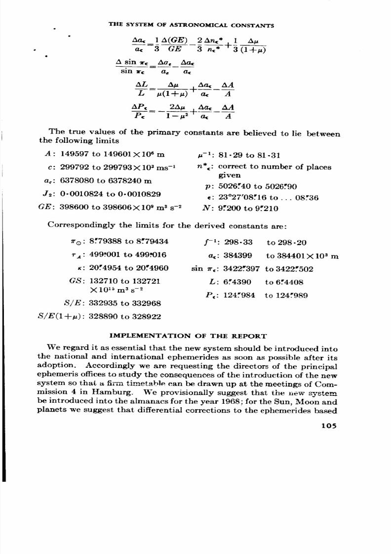
8/7/2019 Significant Achievements in Satellite Geodesy 1958-1964
http://slidepdf.com/reader/full/significant-achievements-in-satellite-geodesy-1958-1964 106/170
THE SYSTEM OF ASTRONOMICAL CONSTANTS
ha, 15(GE) 2An,:* 1 5u
a` 3 GE 3 no* 3 (1-{-tz)
sin T¢ Ao, Aa_
sin w( a, a,
5L A_ An` AA
a` A
AP( 2h_t ha,: AA
Pc 1-u _ a` A
The true values of the primary constants are believed to lie between
the following limits
A : 149597 to 149601X 106 m
c: 299792 to 299793 X 10 _ ms -_
ac: 6378080 to 6378240 m
J_: 0- 0010824 t o 0.0010829
GE: 398600 to 398606X10 g m _ s -2
u-l: 81-29 to 81-31
n*(: correct to number of places
given
p: 5026:40 to 5026."90
_: 23°27'08:16 to... 08."36
N: 9."200 to 9:210
Correspondingly the limits for the derived constants are:
S/E:
S/E(1 +u) :
_o : 8."79388 to 8."79434
r a : 499:001 to 499.016
K: 20."4954 to 20:4960
GS: 132710 to 132721
X 10 is m _ s -2
332935 to 332968
328890 to 328922
jr_ l: 298- 33 to 298- 20
a(: 384399 to 384401X 10 a m
sin Ir¢: 3422."397 to 3422:502
L: 6."4390 to 6:4408
Pc: 124._984 to 124."989
IMPLEMENTATION OF THE REPORT
We regard it as essential that the new system should be introduced into
the national and international ephemerides as soon as possible after its
adoption. Accordingly we are requesting the directors of the principal
ephemeris offices to study the consequences of the introduction of the new
system so that _ m,,_-- t;m_hle....... can be drawn up at the meetings of Com-
mission 4 in Hamburg. We provisionally suggest that the J-,ew system
be introduced into the almanacs for the year 1968; for the Sun, Moon and
planets we suggest that differential corrections to the ephemerides based
105

8/7/2019 Significant Achievements in Satellite Geodesy 1958-1964
http://slidepdf.com/reader/full/significant-achievements-in-satellite-geodesy-1958-1964 107/170
SATELLITE GEODESY
on the current system be tabulated until such time as new or i'evised
theories have been completed.
We intend to meet again at the beginning of the 1964 Assembly so that
we may consider any fresh observational evidence or theoretical argu-
ments that may have been brought to our attention since our meeting in
January 1964. We will then confirm or amend as necessary the list of
constants given above, and this final list will be our recommendation for
the "IAU System of Astronomical Constants." We therefore request
that the Executive Committee submit the following draft resolution for
consideration by Commissions 4, 7, 8, 19, 20 and 31, with a view to its
adoption by the General Assembly:
The International Astronomical Union endorses the final list of constants prepared
by the Working Group on the System of Astronomical Constants and recommends
that it be used in the national and international astronomical ephemerides at theearliest practicable date.
ACKNOWLEDGMENTS
The Working Group wishes to acknowledge the assistance given to the
group by those persons who have responded to our request in a circular
letter dated 30th August 1963 for comments and results relevant to the
system of astronomical constants proposed by the Paris Symposium.
The Group is also grateful to the Astronomer Royal for his hospitality
and for providing facilities for the meeting of the Group at the Royal
Gtvenwich Observatory, Hersttnonceux Castle, on 8-10 January 1964.
W. FRICKE (Chairman)
D. BROUWER
J. KOVALEVSKY
A. A. MIKHA1LOV
G. A. WILK1NS (Secretary)
106

8/7/2019 Significant Achievements in Satellite Geodesy 1958-1964
http://slidepdf.com/reader/full/significant-achievements-in-satellite-geodesy-1958-1964 108/170
I
w m •
Part 5
Determination o] Relative Locations o] Various Areas
of the Earth
Traditionally, geodesy has been concerned primarily
with mapping. An understanding of the terrestrial
gravity field has also been of interest, but largely because
of the necessity of understanding the gravity field
in order to interpret observations of astronomic or
geodetic positioning. That satellite geodesy has re-
versed this emphasis is due primarily to the relative
ease of interpreting satellite orbits in terms of theterrestrial gravity field.
Satellites also provide excellent targets for geodetic
triangulation either through simultaneous observations
or through the use of predicted orbits to connect ob-
servations separated by short periods of time. Both
methods require accurate tiff-ring, good coordination
between observing sites and, to avoid systematic errors,
comparable or identical equipment at each site to be
connected. Good calibration procedures are also im-
portant and for orbit interpolation an accurate knowl-
edge of the satellite motion between observation times
is needed. For these reasons, work in this area is just
starting.
The use of Baker-Nunn observations to improve
station locations is reported in the paper by Izsak
included earlier. The Echo satellites have been very
easy to observe because of their brightness. The U.S.
-Coast and Geodetic Suryey has used observations of
8/7/2019 Significant Achievements in Satellite Geodesy 1958-1964
http://slidepdf.com/reader/full/significant-achievements-in-satellite-geodesy-1958-1964 109/170
J
SATELLITE GEODESY
these satellites for triangulation on the North American
continent and as a planning tool for a worldwide net:
work. For the latter, a much higher satellite will be
needed, however. The following papers include a
report on the use of preliminary observations of Echo I
by French geodesists to tie France and North Africa to
the same reference system, a report on the observation
of a flashing light satellite for geodetic triangulation,
and the results of a test of the SECOR electronic
ranging system for such interconnections. The SECOR
system has the added advantage of providing scale as
well.

8/7/2019 Significant Achievements in Satellite Geodesy 1958-1964
http://slidepdf.com/reader/full/significant-achievements-in-satellite-geodesy-1958-1964 110/170
The following paper is excerpted from a translation of La
Jonction G4od_sique France Mrique du Nord par Photo-
graphics Synchrones du Satellite Echo I. Symposium de
G_<l_ie par Satellites. Institut G_ographique National, 2 °
Direction---G_oddsie, Group d'Etudes Spatiales, December
1964.
N66 37353Q
Geodetic Junction o] France and North A/rica
by Synchronized Photographs Taken From
Echo I Satellite
H. M. DuFouR
Institut Ge'ographique National
I. GENERAL PRINCIPLES OF TRIANGULATION BY SATELLITE
HE BASIC PRINCIPLE is quite simple: a luminous object is seen
against a different background of stars from different points on the
Earth. Photography of this luminous object, together with photography
of the stars which surround it, gives information which permits determin-
ing the position of points on the Earth's surface, other points presumably
being known.
To refine this idea: the solid Earth, considered nondeformable, to which
we attach a trihedron TXYZ, has a known motion on the stellar sphere as
a function of time, a motion given by positional astronomy; knowing the
time means fixing the trihedron in the stellar field; each star thus consti-
tutes an absolute direction in the trihedron TXYZ; a direction given by
the stellar ephemerides.
In a similar fashion, we must fix the luminous object, which, practically
speaking, requires making synchronous (or quasi-synchronous) observa-
tions from the different points on the globe which we want to tie together.
The luminous object can emit flashes of light, thus automatically as-
suring simultaneity, or it may be continuously luminous, making it
necessary to create "artificial flashes" by using synchronously revolving
shutters at the various observation stations.Anna was such a fiashih;ng saW.llite: it has been useful for geodetic ex-
periments. It was more costly than a continuously luminous sateMtc,
it worked only on command, and it is no longer working.
Echo I and Echo II are continuously luminous satellites and Echo I
was chosen for the France-North Africa junction.
109

8/7/2019 Significant Achievements in Satellite Geodesy 1958-1964
http://slidepdf.com/reader/full/significant-achievements-in-satellite-geodesy-1958-1964 111/170
SATELLITE GEODESY
Practically speaking, photography involves:
--A certain number of star photographs to calculate the orientation of"
the camera.
--A certain number of light flashes. In the case of the French observa-
tions, the shutters turned at the rate of 60 revolutions per minute,
producing 60 luminous points per minute, which we call "flashes."
Essentially the problem is to interpolate the position of the flashes
among the known star positions; let us mention immediately that the
60 flashes are reduced to 1 central flash, and that the direction for this
central flash is obtained in the trihedron TXYZ.
Thus each photograph gives a known direction SF, S being the station
and F the fixed point. We shall see how the geodetic problem is treated
for the France-North Africa junction, starting from this fundamentalprinciple.
Several results are necessary for precision:
If an angular precision of 1 second of arc (that is, 1/200 000 of a radian)
is desired for SF, we must have
--A 1-millisecond precision tolerance for the revolving shutter;
--Accuracy of sidereal time to one-twentieth of a second;
--Accuracy within 2 or 3 microns for the determination of the positions
of the stars and of the flashes on the photographic plate (for a focal
length of 30 centimeters).
II. INSTRUMENTS
The apparatus includes, essentially
--A camera of 30-centimeter focal length, furnished with a revolving
shutter and with a leaf shutter.
--A quartz chronometer, to regulate the shutter at the rate of one rps,
for photography of the satellite; and to release the leaf shutter for
the star photographs.
The entire apparatus is extremely simple and highly portable.
Notation of time is done
--For the satellite, by direct reading on the revolving shutter scale:
each second blip of the time signal illuminates the frame of the
shutter, always at the same point, which permits the observer to take
a correct reading (to almost 1 millisecond).
--For the stars: according to the same principle--on a revolving gradu-
ated disk incorporated into the quartz chronometer.
III. THE FRANCE-NORTH AFRICA GEODETIC TIE (MAY 1964)
Under the auspices of the National Center for Space Studies (CNES),
the National Geographic Institute was charged with effecting the France-
110

8/7/2019 Significant Achievements in Satellite Geodesy 1958-1964
http://slidepdf.com/reader/full/significant-achievements-in-satellite-geodesy-1958-1964 112/170
• GEODETIC JUNCTION OF FRANCE AND NORTH AFRICA
Figure/.---Geodetic junction, France-North Africa, by Echo I, May 1964. Points
of the sky photographed, with an indication of successful stations. _ suc-
cessful photograph. ---_ possibly usable photograph. The direction of
the arrow identifies the station. P: Paris Observatory; B: Besancon Observatory.
North Africa tie by means of synchronous photographic observations of
the Echo I satellite. (See fig. 1.)
Known points:
Lacanau (near Bordeaux, on the Atlantic)
Agde (near S&te, on the Mediterranean)
Oletta (Corsica)
Points to be determined:
Hammaguir (West Sahara)
Ouargla (East Sahara)
Actually, the five points are already known in the European Compensa-
tion system (called European Compensation 1950), and the work con-
sists of comparing classical geodetic transfer with transfer by space
geodesy.
111

8/7/2019 Significant Achievements in Satellite Geodesy 1958-1964
http://slidepdf.com/reader/full/significant-achievements-in-satellite-geodesy-1958-1964 113/170
SATELLITE GEODESY
Satellites Used
The only observations retained are those made of Echo I, which, by
reason of its culmination at around 47.5 ° , is well suited to observation
from the Mediterranean area.
The observations took place from the 4th to the 26th of May 1964.
It was sometimes possible to obtain four useful passes in one evening.Echo II was similarly observed beginning May 20, but no observations
have been retained. Echo II could have at most only one useful passage.
Geodetic Configuration
In the final calculations, all the observations of absolute directions will
be replaced by observational relations, which will permit definition of the
unknown points (with their table of errors); but for the observations
themselves, it is necessary to define a general line of work which assures
a priori a satisfactory overall configuration.
One may reason as follows:
First Point oJ View
The central meridian of the observation zone has a longitude of about
2 ° East; the central parallel is at 38 ° latitude. The most important
points for the tie are the points of the satellite's trajectory, on the mean
parallel, to the West and to the East of the central meridian, respectively
(the eastern point is in the zenith in the south of Italy, the western pointsare in the zenith in Spain). These points are determined by intersection
from the three French bases. Their intersection determines the African
points. Considering the diagram, it becomes apparent that this latter
intersection is a good one, the first one not being as desirable, since the
French points constitute a rather narrow base.
Second Point o] View
The set of directions defined with reference to the stars determine a
certain number of planes: these planes, combined, define the lines joining
the points on the ground.
Examining the diagram, one realizes that all the lines are thus well
defined, except the line Ouargla-Hammaguir, as it was difficult to have
African points outside the shadow cone. Here again, one notes that the
African points are defined by an intersection starting from a French base
which is rather narrow.
Forecast of the Passages
For each passage of the satellite, the aiming point on the satellite's
trajectory is, in practice, imposed; the coordinator of the work chooses
this point on the basis of various elements.
112

8/7/2019 Significant Achievements in Satellite Geodesy 1958-1964
http://slidepdf.com/reader/full/significant-achievements-in-satellite-geodesy-1958-1964 114/170
GEODETIC JUNCTION OF FRANCE AND NORTH AFRICA
--First of all, is the necessity for a generally well formed geometric
" figure, as we have noted.
--Observation time suitable for star photography: from this point of
view, the stations at high latitudes are very unsuitable in summer.
--It is also necessary that the satellite leave the shadow cone soon
enough that the observers are not surprised (in practice, the time of
the satellite's arrival often cannot be predicted to better than about
5 minutes).
Theoretically, it should be possible to take into account previous success-
ful evenings of observation, but practically, this is hardly possible; in fact,
the general coordinator establishes a plan and follows it more or less rigidly.
For the predictions, the Echo I ephemerides furnished by the Smith-sonian Astrophysical Observatory in Massachusetts are used.
Upon reception of an ephemeris, the passages are numbered, the
ephemeris is extrapolated for about 15 days, and the points of passage
are chosen (that is, the points in the sky at which the ballistic cameras
will have to be aimed). An electronic program then furnishes a statement
indicating for each station all the elements of the observations.
In practice, between the elements of the extrapolated ephemeris and
the values from the following ephemeris, we currently encounter differ-
ences on the order of 10 minutes in time and 2 ° to 3* in longitude. These
differences, although disagreeable, are acceptable for the observations.
They underscore the fact that Echo I, being very light, is extremely
sensitive to radiation pressure.
Field Operations
The task of taking the pictures requires only two operators, but in
practice it is a good idea to provide a team of three, since, during the
usable time period, photographs are taken every 2 hours during the night,every night. It is desirable under these conditions to provide one night's
rest every three nights for each operator.
The picture-taking operation includes the following phases:
--Placement of the camera in the station 2 hours before the observa-
tion, and starting the chronometer
--Loading a plate in the camera
--Setting the chronometer, by time signals
--Photography of the stars (first exposure)
---Starting the shutter disk; regulation by time signals
--Photography of the satellite, at the rai_ of onc e.._,_p______mer second,
except for the 60th-second blip of each minute, which is eliminated
by a disk manipulated by an operator 1
1The operator hears the time signals and places the disk in front of the objectivewhen he hears the long signal of the full minute.
113

8/7/2019 Significant Achievements in Satellite Geodesy 1958-1964
http://slidepdf.com/reader/full/significant-achievements-in-satellite-geodesy-1958-1964 115/170
SATELLITE GEODESY
--Stopping the disk: photography of the stars (second exposure)
--Photography of the synchronizing marks at the base of the camera
--Replacing the plate
--Setting up the camera for the next observationOperations also include:
--Development of the plate
--Recording the following information: direction of the satellite's
passage, notation of the minutes.., direction of diurnal movement.
The important elements of field operations are essentially
--The stability of the apparatus during the interval of time which
separates the two photographs of the stars; this interval is presently
15 minutes, and will be reduced to less than 10 minutes.--Recording the time on the revolving shutter, which must be done
with an accuracy within 1 millisecond.
Success of the Observations
About 60 positions of the satellite were selected in advance to be photo-
graphed (each comprising 60 points). Here is the tabulation of successful
photographs :
H:unmaguir: 15 Ouargla: 40Olctta: 40 Agde: 35
Lacanau: 25
Naturally, every point photographed simultancously by at least two
stations is usable. Theoretically, the probability of one position in five
successful negatives is:
15 40 40 "-_' 35 X 25 f_.s I
(In fact, there were only two entirely successful points out of 60.)
IV. PROCESSING THE PLATES--CALCULATIONS
We cannot go into the complete details of this last phase of the work
here. We only indicate the fundamental subdivisions, which involve the
following operations:
(A) Calculations of the theoretical coordinates of the stars on the plates
(B) Measurement of the plates with a comparator
(C) Calculations of the formulas giving the direction cosines of tileflashes in the terrestrial Cartesian system
(D) Intersection of the flashes from the approximate coordinates of the
stations
(E) Caldulations of the unknown coordinates of the stations from the
known coordinates.
114

8/7/2019 Significant Achievements in Satellite Geodesy 1958-1964
http://slidepdf.com/reader/full/significant-achievements-in-satellite-geodesy-1958-1964 116/170
GEODETIC JUNCTION OF FRANCE AND NORTH AFRICA
The characteristics of these various operations are given in the follow-
irfg pages. All the calculations were made on the CAB 500 of the
Geographic Institute.
Other Calculations
In addition, the coordinates of the tie points in the terrestrial Cartesian
system were carefully established by means of classical geodesy.
Planar coordinates, the geographic coordinates (kq_) for North Africa in
the European Compensation system, are available; their accuracy is
close to 10 meters.
Altitudes, the altitudes H of the different points above the International
Ellipsoid, are calculated by integration of the deviations of the verticalat the astronomic points.
First calculation: French network
Second calculation: Southern France, Italy, Spain, North Africa
The French network is dense enough to make the results worthy of
confidence. The second network is made up of points rather distant
from each other. After cross-checking, it may be estimated that 1-
decameter precision is preserved here as well.
The calculation is carried out by astronomic leveling, establishing the
relations by observations between each point and its nearest neighboring
points. We assume that each difference of level has an error independent
of the others and proportional to the distance; these hypotheses are not
absolutely rigorous. It is proposed to include calculations statistically
more valuable, which are presently being undertaken.
The approximate coordinates of the stations (calculations D and E) are
furnished by the terrestrial Cartesian coordinates, derived from the
coordinates (),¢H), calculated on the International Ellipsoid.
(A) Calculation of theoretical coordinates of the stars on the plates
Ecliptic coordinates 1950; XEYEZE
Selection of stars:
Calculation of XYZ ecliptic coordinates of the camera for 1950
Rejection of stars by studying the scalar product:
XXB+ YYE+ZZB
115

8/7/2019 Significant Achievements in Satellite Geodesy 1958-1964
http://slidepdf.com/reader/full/significant-achievements-in-satellite-geodesy-1958-1964 117/170
SATELLITE GEODESY
Reduction of the selected stars to (p, q, r) direction cosines in the"
terrestrial Cartesian system
Transformation into the local horizontal system:
(-)h =R1 q
zh r
Refraction
Transformation into the plate system:
= R_ Yh
Zh
(f= focal distance)
l OUTPUT l
TAPE PRINTED FORM
OPERATION C OPERATION B
DZ: zenith distance
AZ : azimuth
UT: universal time for the stars
UT: universal time for the flashes
P: pressure _ - "r "T : temperature_ Ret
actlon
(B) Measurement of the plates with the comparator
The measurement of a plate requires, in practice, a day's work for two
operators. It must be done very carefully.
The operators use the approximate coordinates (xcyc), given by calcu-
lation A, to position the plate under the comparator.
Then they note the elements of the plate in the following order:
--Synchronizing marks at the bottom-]
of the camera _ Operator 1, operator 2--Stars acting as secretary
--Flashes
--Flashes 1
--Stars Cperator 2, operator 1
--Synchronizing marks at the bottom acting as secretary
of the camera
116
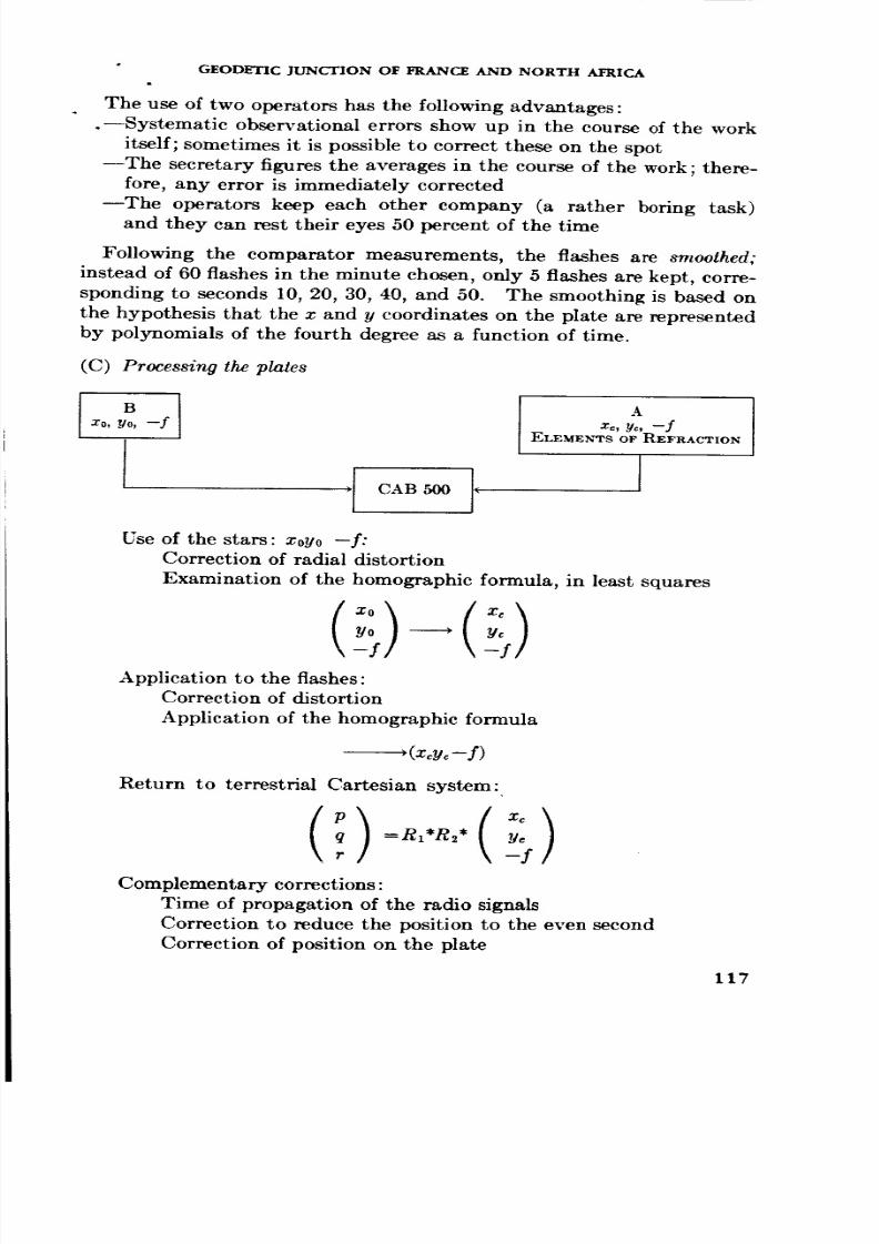
8/7/2019 Significant Achievements in Satellite Geodesy 1958-1964
http://slidepdf.com/reader/full/significant-achievements-in-satellite-geodesy-1958-1964 118/170
GEODETIC JUNCTION OF FRANCE AND NORTH AFRICA
The use of two operators has the following advantages:
.--Systematic observational errors show up in the course of the work
itself; sometimes it is possible to correct these on the spot
--The secretary figures the averages in the course of the work; there-fore, any error is immediately corrected
--The operators keep each other company (a rather boring task)
and they can rest their eyes 50 percent of the time
Following the comparator measurements, the flashes are smoothed.
instead of 60 flashes in the minute chosen, only 5 flashes are kept, corre-
sponding to seconds 10, 20, 30, 40, and 50. The smoothing is based on
the hypothesis that the x and y coordinates on the plate are represented
by polynomials of the fourth degree as a function of time.
(C) Processing the plates
iAi_, y_, --fxo, yo, -f ELEMENTS OF REFRACTION
Use of the stars: xoyo --f:
Correction of radial distortion
Examination of the homographic formula, in least squares
Application to the flashes:Correction of distortion
Application of the homographic formula
--_(_cuc-/)
Return to terrestrial Cartesian system:
Xc
Complementary corrections:
Time of propagation of the radio signals
Correction to reduce the position to the even second
Correction of position on the plate
117

8/7/2019 Significant Achievements in Satellite Geodesy 1958-1964
http://slidepdf.com/reader/full/significant-achievements-in-satellite-geodesy-1958-1964 119/170
SATELLITE GEODESY
Printing of a tape:
P
q of the flashes and elements P, T
r for refraction
(D) Intersection. Several simultaneous plates give a series:
Plate 1 Plate 2
+kAB 5O0 1+
Plate 3
C3
First least squares calculation, without weighting, and without correction forrefraction
--+Approximate coordinates of the flashes.
Second calculation, with weighting, and with correction for refraction
--*Coordinates XFYFZF, the most coherent as a function of the coordinates ofthe stations.
Printing of a tape
Operation E
(E) Geodetic calculation
Regrouping of the series: each plate itself gives two observational rela-
tions in a general system of least squares.
For these relations, tile smoothed values of tile central flash is used.*
For each plate:
l)proximate coordinates of the
centr'd flash o,'ientation (p q r) of
the central flash P and 7' for
calculation of refraction
irection of the sun
Approximate coordinatesof the stations
Connections between the
stations
)I CAB500 1+
*Ill a more elaborate program, 10 relations will be written corresponding to the 5
smoothed directions (seconds 10, 20, 30, 40, 50) with their table of variances.
118

8/7/2019 Significant Achievements in Satellite Geodesy 1958-1964
http://slidepdf.com/reader/full/significant-achievements-in-satellite-geodesy-1958-1964 120/170
G
GEODETIC JUNCTION OF FRANCE AND NORTH AFRICA
For each flash:
Refraction correction
Phase correction
Establishment of the observational relationNormalization
Elimination of the flash coordinates
Summation of the equations:
(1) resulting from a priori connections between the station
points (known points, known distances, etc.)
(2) resulting from the normal equations, after elimination of
the flashesTable N of weights of the coordinates
Table N -1 of the variance. Calculation of mean quad-
ratic error of a direction
Coordinates of the stations
V. RESULTS OBTAINED AND PLANNED IMPROVEMENTS
In a general way, the Geographic Institute has been occupied with the
production of highly transportable equipment, and with effective expe°
rience; we hope in the future to perfect the various operations progres-
sively, according to the successive problems which increased precision
poses.
At present, we expect from the France-North Africa experience a
theoretical angular precision of 1/100 000 of a degree (that is, two arc-
seconds) which corresponds, in gross fashion, to a precision of 20 m be-
tween the extreme geodetic points. It is not yet possible to say anything
definitive about the practical results, the first of which are just beginningto appear (operation D). 2
We hope in the future to increase the precision of the measurementsas follows:
--Regulation of the entire picture-taking operation by a quartz
chronometer; currently, this clock assures regular rotation of the
shutter disk, but not its time setting, which is done directly from the
time signals. In the future, the chronometer will also set this time,
being regulated itself, by different time signals, before and after
phut_graphy of the ._tellite and of the stars. This latter operation
may thus be cut down to less than 10 minutes.
2The sightings of series 6 (longitude 13° E, latitude 40 °) intersect with a radialuncertainty of 10 m, an excellent result if one considers that the mean distances are2000 kin.
119

8/7/2019 Significant Achievements in Satellite Geodesy 1958-1964
http://slidepdf.com/reader/full/significant-achievements-in-satellite-geodesy-1958-1964 121/170
SATELLITE GEODESY
--I"o use thick photographic plates (6 mm), rigorously flattened.
--To use fast emulsions, in order to increase the number of stars
recorded in one session.
--To take two exposures of the stars before and two exposures after-
ward.--To place two cameras in parallel in each station systematically:
this procedure improves the precision of the directions in the ratio
v/2 and permits the easy disclosure of any discrepancy.
--To air-condition, at least partially, the picture-taking apparatus
and the quartz clock.
120
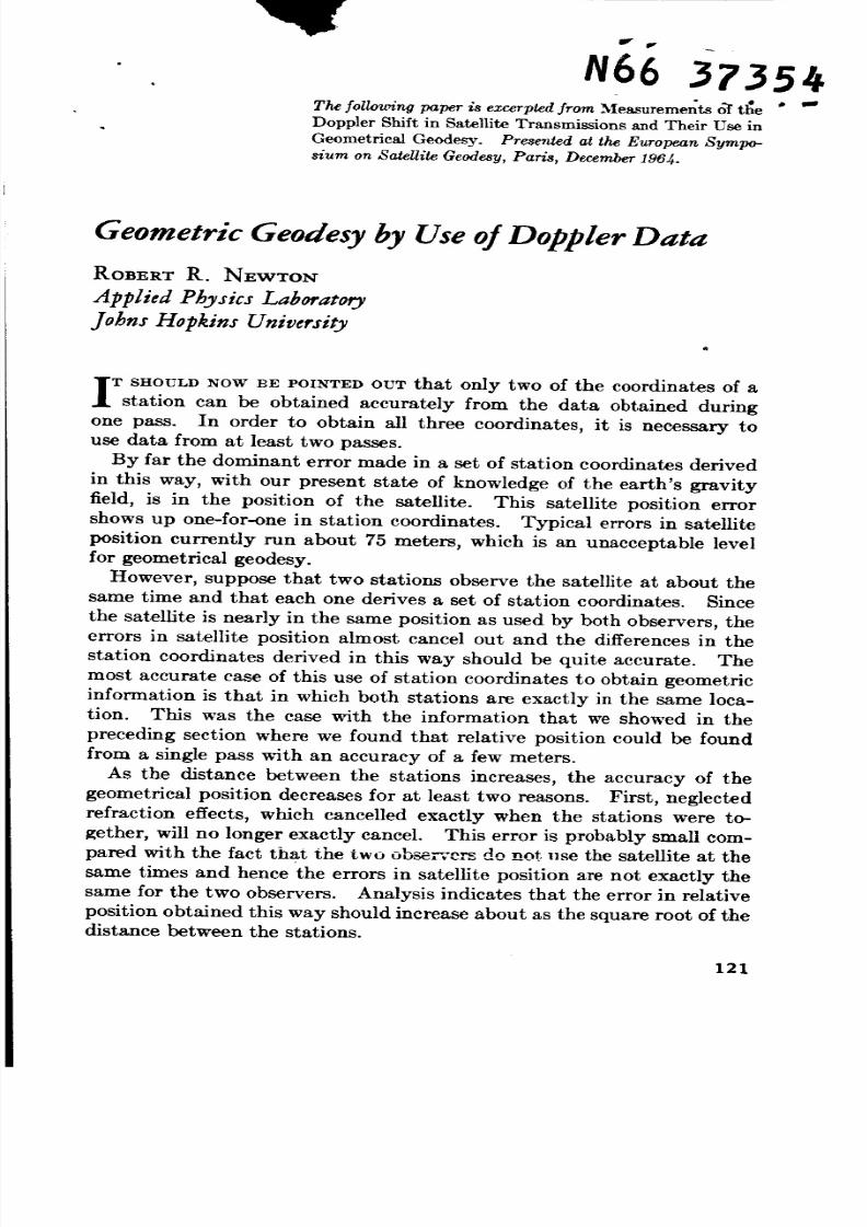
8/7/2019 Significant Achievements in Satellite Geodesy 1958-1964
http://slidepdf.com/reader/full/significant-achievements-in-satellite-geodesy-1958-1964 122/170
tr"
N66 37354
The followin 9 paper is excerpted from Measurements _ ti_e •Doppler Shift in Satellite Transmissions and Their Use in
Geometrical Geodesy. Presented at the European Sympo-Mum on Satellite Geodesy, Paris, December 1964.
Geometric Geodesy by Use oJ Doppler Data
ROB_.RT R. NEWTON
Applied Physics Laboratory
Johns Hopkins University
T SHOULD NOW BE POINTED OUT that only two of the coordinates of astation can be obtained accurately from the data obtained during
one pass. In order to obtain all three coordinates, it is necessary to
use data from at least two passes.
By far the dominant error made in a set of station coordinates derived
in this way, with our present state of knowledge of the earth's gravity
field, is in the position of the satellite. This satellite position error
shows up one-for-one in station coordinates. Typical errors in satellite
position currently run about 75 meters, which is an unacceptable level
for geometrical geodesy.
However, suppose that two stations observe the satellite at about the
same time and that each one derives a set of station coordinates. Since
the satellite is nearly in the same position as used by both observers, the
errors in satellite position almost cancel out and the differences in the
station coordinates derived in this way should be quite accurate. The
most accurate case of this use of station coordinates to obtain geometric
information is that in which both stations are exactly in the same loca-
tion. This was the case with the information that we showed in the
preceding section where we found that relative position could be found
from a single pass with an accuracy of a few meters.
As the distance between the stations increases, the accuracy of thegeometrical position decreases for at least two reasons. First, neglected
refraction effects, which cancelled exactly when the stations were to-
gether, will no longer exactly cancel. This error is probably small com-
pared with the fact that the two observcm do not use the satellite at the
same times and hence the errors in satellite position are not exactly the
same for the two observers. Analysis indicates that the error in relative
position obtained this way should increase about as the square root of the
distance between the stations.
121

8/7/2019 Significant Achievements in Satellite Geodesy 1958-1964
http://slidepdf.com/reader/full/significant-achievements-in-satellite-geodesy-1958-1964 123/170
SATELLITE GEODESY
The method of simply extracting station coordinates is equivalent to
using data from one station to correct the position of the satellite and
using this corrected satellite position to give the position of the other
station. The computed satellite orbit, of course, will contain velocity
errors as well as position errors and it is these velocity errors which cause
the relative station position error to increase with the distance between
the stations. The accuracy of relative information can therefore be in-
creased if data from three or more stations at about the same time are
used. In effect, what we can do then is to use information from two of
the stations to correct both position and velocity errors in the satellite
orbit and thus improve the accuracy of the third station relative to the
other two. In practice, of course, one would probably treat the data
from all three stations simultaneously, varying the orbit and the stationcoordinates until the best fit to alI the data is found. The differences in
station coordinates would then represent accurately the lengths of the
chords joining the three stations.
Analysis of doppler data by this method has been carried out by
Anderle and Oesterwinter (Ref. 5) using data from six TRANET stations
within the continental United States. The comparison of the set of
chord lengths derived in this way and that derived from ground survey
is shown in figure 1, based upon data from about thirty passes. The
..... T r
_ / 450
-- 40o
35 o
300
250
120 115 110 105 100 95 90 8.5 80 75
Figure /.--Comparison of chord lengths derived from ground survey and from
doppler observations.
122

8/7/2019 Significant Achievements in Satellite Geodesy 1958-1964
http://slidepdf.com/reader/full/significant-achievements-in-satellite-geodesy-1958-1964 124/170
p
GEOMETRIC GEODESY BY DOPPLER DATA
n_mber accompanying each chord in this figure is the discrepancy in
meters between the two values of chord length. Figure 1 is copied from
reference 1 with the permission of the authors.
Results of at least equivalent accuracy should be obtained using theintegral doppler receiver, since studies of the TRANET stations show
that they have about the same instrumental errors.
Except for the chords that terminate at Station 003 in New Mexico,
no discrepancy exceeds 20 meters, and most are considerably less. The
comparatively large errors involving Station 003 caused the location of
that station to be investigated again. It has been found that the station
antenna was moved several times, in order to improve signal reception,
without notification being sent to the analysis center. At the present
time, we are trying to trace the time history of the antenna location to
see if Station 003 results can be made consistent with other results.
We have considerable confidence in the accuracy of the satellite results
because of an incident connected with Station 710. The original results
for this station showed an east-west discrepancy of about 30 meters.
This discrepancy was traced to a card-punch error of exactly 1W in the
longitude of the station. The results shown in figure 1 were obtained
after correcting this card-punch error.
In summary, the relative horizontal position of two stations within afew hundred kilometers of each other can be obtained, using the doppler
data from a single pass, with a standard deviation of about 10 or 15
meters. By the use of more passes, all three coordinates of the relative
position can be determined, and with a higher accuracy. Across the
dimensions of a continent, using four or more observing stations, relative
positions can be obtained in all three dimensions with a confidence level
of about 10 meters, using a modest number of passes.
I_-_'_R_NCE
l. ANDERLE, R. J.; AND C. OESTER_rlNTER: "A Preliminary Potential for the Earth
From Doppler Observations on Satellites," U.S. Naval Weapons Laboratory,
May 1963.
123

8/7/2019 Significant Achievements in Satellite Geodesy 1958-1964
http://slidepdf.com/reader/full/significant-achievements-in-satellite-geodesy-1958-1964 125/170
w
On October 31, 1962, the Department of Defense la_mched the first satellite
designed primarily for geodesy. This permitted the testing of several optical
and electronic techniques for precise geodetic satellite tracking. The follow-
ing papers describe the satellite design and describe the results ofobservations
of the flashing light which this satellite carried. Observations of the doppler
frequency measurements are included in the results of doppler tracking
reported e_trlier.

8/7/2019 Significant Achievements in Satellite Geodesy 1958-1964
http://slidepdf.com/reader/full/significant-achievements-in-satellite-geodesy-1958-1964 126/170
N55 37355ThefoUowinq paper is a chapter from The Use of A,rtifaeiab BSatellites for Geodesy, G. Veis, eel., North-Holland Pub-
lishing Co. (Amsterdam), 1963, pp. 255-_60.
Project ANNA
MAv._ M. MACOM_ER
Bureau of Naval Weapons, Department of the Navy
Department of Defense, Washington, D.C., U.S.A.
ROJECTANNA is x UNITED STATES geodetic satellite program. The
name ANNA is an acronym for Army, Navy, NASA (the National
Aeronautics and Space Administration), and Air Force, the agencies that
originally collaborated on formulating the program or that were expected
to participate actively in the observation program. When the geodetic
satellite program was first proposed, the Department of Defense feared
that the output of the program, in addition to being of a scientific nature,
might be of critical military significance. The program was therefore
temporarily classified, and as a result, NASA participation did not
materialize. Recently a review of the program and its expected results
has been made, and the classification has been removed, opening the pro-
gram to participation by NASA and, through them, by the world-wide
scientific community.
The belief that the scientific community should participate in ANNA
was so firm to the people who formulated the program that in mid-1960 a
provision was made to allocate 50% of the available light-flashes from the
optical beacon to a scientific program administered by NASA.
The first ANNA satellite is scheduled to be launched into a near-circu-
lar orbit inclined 50 ° to the equator, with an altitude of one megameter.
At present, only two launches are authorized, the second being scheduled
as a backup to the first in order to ensure a successful orbit and to providea sufficiently extended period of observation to produce significant data.
The satellite contains three basic types of instrumentation that will be
used for obtaining positioning information. For range determination, a
tmnspender in the satellite is coupled with ground instrumentation that
makes a phase comparison between a modulating frequency as transmitted
to and as returned from the satellite. Three frequencies in the vhf-uhf
bands are used: one for transmission to the satellite, and two coherent
frequencies for transmission from the satellite to ground. Analysis of the
125

8/7/2019 Significant Achievements in Satellite Geodesy 1958-1964
http://slidepdf.com/reader/full/significant-achievements-in-satellite-geodesy-1958-1964 127/170
SATELLITE GEODESY
difference in phase shift on the two returning frequencies permits a cor-
rection to be made for refraction effects. To resolve any ambiguities in
distance measurements, four different modulating frequencies are em-
ployed. The satellite transponder receiver is energized at all times, but
the transmitters are turned off except when the satellite is being inter-
rogated. Power limitations within the satellite restrict interrogation to
six or seven passes per 24 hours; the satellite is thus adequate for use by
only one complex of ground stations. In an attempt to keep the satellite
instrumentation as simple as possible, the ground stations are tied together
by a VLF timing net, and transmit in bursts such that the signals from
the various ground stations are received at the satellite sequentially.
The highly complex ground instrumentation necessary to accomplish the
interrogation and measurement functions, coupled with the limitationon power available for the transponder, make this system unavailable to
the scientific community.
For optical determination of satellite topocentric direction, a high-
intensity optical beacon is used; when activated, it produces a series of
five light-flashes spaced 5.6 seconds apart. The main advantage of the
optical beacon is that when it is flashed, an infinite number of observers
within the circle of visibility can observe the light with relatively simple
equipment, making this system of maximum benefit to the scientific
community. One drawback of the optical system is that the powerconsumption of the beacon is very large, limiting the number of flash
sequences per day to about 20 or less, depending on the exposure of the
satellite to sunlight to recharge the battery. Because of this power
limitation, light flashes cannot be programmed for everyone who might
desire to participate in tile program, but must be programmed to provide
the maximum return in geodetic knowledge. The result is that certain
observers will not be able to use the light when most convenient for them,
although they will be able to observe it at other times even though the
geometry of position solutions will not be optimum.
Range rate information is obtained by observing the doppler shift of
ultra-stable transmissions of the satellite. Four frequencies will be
broadcast continuously for this purpose. The pair of frequencies
designed for geodetic measurements will be 162 and 324 Mc, with another
pair, 54 and 216 Mc, reserved for refraction studies and for a possible
backup in case of failure of the prime tracking frequencies. All four of
the frequencies are coherent, so tracking could be accomplished using
any two. Since transmitters are of low power drain, they can be left oncontinuously, and thus be available to observers throughout the world.
The ground instrumentation for receiving the signals and counting the
doppler shift imparted to the signal is complex and may be a deterrent
to observations by the scientific community.
126

8/7/2019 Significant Achievements in Satellite Geodesy 1958-1964
http://slidepdf.com/reader/full/significant-achievements-in-satellite-geodesy-1958-1964 128/170
I
PROJECT ANNA
The temperature-controlled crystals that drive the ultra-stable trans-
mitters are also used to run a satellite-borne clock. Approximately
every 90 seconds, time signals are broadcast from the satellite as phase
modulation on two of the doppler signals. By keeping track of the fre-quency drift of the crystals, as obtained by the doppler tracking stations,
it is possible to correct the time of transmission of these signals to better
than 0.5 millisecond. Since the same clock that provides these timing
signals also initiates the flash sequences for the optical beacon, the
doppler and optical observations are tied together in time.
The small satellite memory consists of 22 sixteen-bit words. Injected
into it are the two's complement of the identification of the 5.6-second
timing pulse that should initiate each light-flash sequence. Every 5.6-
second timing pulse generated by the satellite clock is added to each of
the first 21 words, and when each word overflows a light-flash sequence
is initiated.
The satellite is oriented with the earth's magnetic field so that the pole
of the satellite visible from earth is a function of the geomagnetic latitude
of the satellite. Two beacons face the north pole of the satellite, and two
face the south pole. Only 15 bits of the 16 in each word in the memory
are used for light-flash timing. The 16th bit has injected into it an
indication of whether the north or south lights should be flashed. The22nd word of the memory will not initiate flash sequences, but is used
for telemetry purposes to indicate whether or not the lights did flash
as planned.
In addition to the geodetic systems instrumentation, the satellite con-
tains various minor experiments that test the environment and the
attitude of the satellite.
During the first three months after launch, an intensive calibration
program will be undertaken, wherein the three types of measurementswill be compared among themselves, and with terrestrial survey results.
This calibration program is considered of prime importance to prove that
no biases exist in any of the instrumentation used or in the methods of
data handling that are utilized. If any biases do exist, they must be
eliminated or corrected before any geodetic program can be undertaken
on a world-wide scale. Upon successful completion of the calibration
phase, a world-wide geodetic observation prograpa will be undertaken with
the intent of refining our knowledge of the earth's gravitational field and
of providing the location of tracking stations relative to the earth's
center of mass.
Now that the entire program has been declassified, NASA can partici-
pate in the observation program, and can coordinate the participation of
foreign and domestic scientific interests. Neither details of observation
127

8/7/2019 Significant Achievements in Satellite Geodesy 1958-1964
http://slidepdf.com/reader/full/significant-achievements-in-satellite-geodesy-1958-1964 129/170
SATELLITE GEODESY
equipment to be used, nor a modus operandi has yet been crystallized,
but the following plans for participation are under active eonsiderati6a:
1. use of the Smithsonian Astrophysical Observatory optical network;
2. use of the MOTS (Minitrack Optical Tracking System) cameras
located at most of the NASA minitrack stations;
3. use of minitrack interferometry information;
4. use of the NASA-Jet Propulsion Laboratory radar systems for
space probes;
5. voluntary participation of interested observatories.
Because of the power limitation for the optical beacon, only selected
observatories that would add strength to the present planned deployment
of tracking equipment can be considered for use in this program as far as
special programming of the light is concerned. This does not in any way
limit participation by all observatories within the area of visibility of each
flash sequence, but it does mean that certain observatories will not derive
the benefit of optimum geometry. All contact with civilian observers will
be through the NASA. Details of this observation program will be
promulgated to all interested persons as soon as they are made firm.
At the present time, two satellites have been fabricated. They have
completed comprehensive tests, performing perfectly all the while. These
two satellites are currently undergoing extensive checkout after the
shipment and are being fitted out to the launch vehMe.
The activity collecting dattt will reduce and preprocess the data to
eliminate any spurious dat._ points,.if the facilities are availatfle. Since
many independent observers will be unable to carry out this function,
provisions must be made to handle reduction of data and elimination of
spurious points at some central activity. Data will then be processed
to produce a unique reference frame within the earth, to determine the
earth's gravitational field, and to provide geocentric locations of tracking
stations.The two planned launches, which together assure essentially one orbit
of sufficient lifetime, are of course insufficient to meet the needs of any
geodetic program. Some planning has taken place on the variety of
orbits that would be of value to any program of this sort, and that are
feasible from existing launch sites with existing boosters in the moderate
price field.
128

8/7/2019 Significant Achievements in Satellite Geodesy 1958-1964
http://slidepdf.com/reader/full/significant-achievements-in-satellite-geodesy-1958-1964 130/170
The following paper is excer#e_t from The Use of a Flashing
Light Satellite for Datum Interconnection. Presented at
the DIA Conference, Washington, D.C.,-Oc_ober28-30, 196-L
N66 3?356
Results From Satellite (ANNA) Geodesy
Experiments
OwE_ W. WILLIAMS, PAUL H. DIS_ONG,
AND GEORGE HADGIGEORGE
Terrestrial Sciences Laboratory
Air Force Cambridge Research Laboratories
INTRODUCTION
x 31 OCTOBER 1962 with the launch of the Satellite ANNA 1-B intoa nearly circular orbit of approximately 600 nautical miles, a new
era in the sciences of photogrammetry and geodesy was started (ref. 1).
This geodetic satellite (designed for six months' operation) continues to
be reproductive some 24 months later. The name ANNA reflects its
four United States sponsors, the Air Force, Navy, NASA and the Army.
The Army was responsible for the electronic ranging system known as
SECOlq ; the Navy was responsible for the electronic doppler system and
integration of the satellite payload; the Air Force was to develop the
flashing light system; and NASA was to assist in the optical observa-
tional program. This paper will cover only those aspects contributingto the optical phases of the active ANNA program.
In January 1963, after more than two months of excellent performance,
a defective capacitor bank caused a malfunction in the optical system.
The output of the light system was reduced to abottt 25% to 30_ of its
original value and this condition remained in effect into July. Therefore,
between January and July only a limited program of flash transmissions
transpired and while usable camera data was still received it was for the
most part not up to original expectations.
Prior to the capacitor problem in the satellite, geodetic stellar cameras
obtained an excellent series of photographs. The image diameter of the
fl_sh recorded on 103-F emulsion averaged 70 microns on the PC-1000's
and approximately 50 microns on the BC-4-300 plates. In mid-July
1963, the light output returned to normal and good data were again
129

8/7/2019 Significant Achievements in Satellite Geodesy 1958-1964
http://slidepdf.com/reader/full/significant-achievements-in-satellite-geodesy-1958-1964 131/170
SATELLITE GEODESY
obtained. Because of normal solar cell deterioration, only 7 flash
sequences a da y can currently be programmed as opposed to the original
30 sequences.
Due to the condition of the main battery controlling the command
system and the lack of doppler trackingdata, the Applied Physics Labora-
tory, Johns Hopkins University, suggested t o Air Force Cambridge
Research Laboratories in October 1963 that we operate the flashing light
by employing our alternate optical logic. The emergency over-ride
system (EMOS) was developed to provide the necessary redundancy for
the optical operations and this bit of foresight continues to pay dividends.
The EMOS system consists of a World timing system accurate to one
millisecond, a transmitter, a linear amplifier, and an antenna system.
DESCRIPTION OF BEACON
The ANNA optical beacon, developed for AFCRL by Edgerton,
Germeshausen and Grier (EG&G), consists of two pairs of xenon filled
stroboscopic lamps with reflectors, one pair on the north face of the solar
cell panel and one pair on the south face (Figure 1). When either set
Figure 1.-A close view of one of the four
strobe lights located on the A NN A geo-
detic satellite.
of lights is triggered by the satellite memory (no longer possible) or by
EMOS, a series of 5 flashes is produced. An enlargement of a part of
one of the first photographs of ANNA clearly demonstrates the above
mentioned spacing (Fig. 2).
LIGHT INTENSITY
The light intensity of the ANNA beacons is not constant over the
light angle but varies as shown by a dotted line in Figure 3 while the
solid line shows the intensity used t o predict the image sizes for ANNA.
130

8/7/2019 Significant Achievements in Satellite Geodesy 1958-1964
http://slidepdf.com/reader/full/significant-achievements-in-satellite-geodesy-1958-1964 132/170
RESULTS FROM SATEJJ-ITE GEODESY EXPERIMENTS
Figure .?.-ANNA 1-B strobe light images. Copy of photograph taken during
test to check optical system developed by Air Force Cambridge Research Lab-
oratories. Satellite photographed at 0 3 5 0 hr e.s.t. as it crossed Boston area
with BC-4, 300-mm FL camera. Images on plate.
VALIDITY OF EQUATIONS
During the development phase of A S S A , the image sizes on Air Force
PC-1000 geodetic stellar camera plates were predicted for conditions of
moderate haze. Currently, two groups, EG&G and Duane Brown
Associates, Inc., have examined some of the AKYA PC-1000 plates t o
determine the validity of the equations.
Duane Brown Associates analyzed 88 images on 20 different plates
taken from six different PC-1000 cameras (ref. 2). The plates were
selected t o be representative of different cameras, different locations, and
a wide range of image diameters.The key results of the study are
summarized in Table 1. Both groups obtained good agreement between
computed and measured image sizes. There were four cases in which
cameras 104 and 121 were employed in side-by-side operations. The mean
image diameters from 104 turn out to be consistently and significantly
larger than those from 121. This convincingly demonstrates tha t signifi-
cant differences may exist in the capabilities of cameras of the same type.
On the \\-hole, agreement between theory and observation is considered
to be sufficientll- good (13.4 micron mean errorj for the theory t o be
nsed fe r pl?r,noses of genera! planIling
INTERVISIBLE OBSERVATIONS
Simultaneous photographic observations were made by ten -1ir Force
PC-1000 cameras during the period September 1963 t o January 1961.
131

8/7/2019 Significant Achievements in Satellite Geodesy 1958-1964
http://slidepdf.com/reader/full/significant-achievements-in-satellite-geodesy-1958-1964 133/170
SATELLITE GEODESY
10
L3
_s
.,J
Q
Z 7
5o
6
Z 5tA/F--Z
0
3
/
//
/
J\
\
%
\\\
\
Uted Foe Image Colculatlonl
True Value Of Intenelty
0° t0° 20° 30° 40° 50° 60° 70° 80° 90 °
LIGHT ANGLE (0)
Figure 3.--Light beam pattern.
Geodetic position determinations using these ANNA 1-B observations
indicate that the PC-1000 camera system used with the intervisible
technique is capable of extending geodetic control to a proportional
accuracy of better than 1/100,000.
Sixty observation nets were obtained in the Gulf Test. A net is
defined as a flash sequence which was successfully photographed from
three or more camera stations. Six nets were used to test the capabilities
of the PC-1000 cameras. (See Table 2.)
The 1381st Geodetic Survey Squadron of AFCS provided the coordi-
nates of the camera sites which were tied to first order control of the North
132

8/7/2019 Significant Achievements in Satellite Geodesy 1958-1964
http://slidepdf.com/reader/full/significant-achievements-in-satellite-geodesy-1958-1964 134/170
RESULTS FROM SATELLITE GEODESY EXPERIMENTS
C_
I.
e_ e., =
_._
_'_
_ °._
_-_n _ .._ 1:::I
_'-_
.... _-E
"T _7g+7 _+7ST+S+Sgg7 _
1.33

8/7/2019 Significant Achievements in Satellite Geodesy 1958-1964
http://slidepdf.com/reader/full/significant-achievements-in-satellite-geodesy-1958-1964 135/170
o,_
el
SATELLITE GEODESY
¢.D_.Dc.Oc.Oc.D¢_
134

8/7/2019 Significant Achievements in Satellite Geodesy 1958-1964
http://slidepdf.com/reader/full/significant-achievements-in-satellite-geodesy-1958-1964 136/170
RESULTS FROM SATELLITE GEODESY EXPERIMENTS
American Datum (NAD 1927). ACIC supplied the geoid-spheroidseparations necessary to convert heights above mean sea level to heights
above the reference spheroid.
35 - -_-
' ': -- [ !64
i 640 • ,, \
Figure &--The coordinates of station 640 are determined from those of
stations 648 and 649 by nets 30 and 54.
Table 3.--Geodetic Position Determination of Station 640 From Stations
648 and 649
Reference stations 648 and 649 a_-s =¢E-w =art =0
Input standard deviations station 640 a_c-s = 100 m, aE-w--100 m, _u = 5 m
Input error station 640 ¢ = +3"; ), --- --4"
Observations: All stations observed 5 flashes each on nets 30 and 34
Average observation a used: 648, :85; 649, 1._08; 640, 1:56
North American Datum 27
ANNA Data Reduction
R = [(Ax)=+ (by)' + (5z)'] '/'
$ S t 1 1
R, =[,,, +_,,+_,] /
X H(meters) R(meters)
29°33'44:80 90°40'44:19 7.0
44:78 43.*93 7.6
:O2
:11
:26
:25
--.6
4.8
7.1
8.7
Distance: 987 km
Proportional Accuracy (NAD Standard) 1/140,000
135

8/7/2019 Significant Achievements in Satellite Geodesy 1958-1964
http://slidepdf.com/reader/full/significant-achievements-in-satellite-geodesy-1958-1964 137/170
SATELLITE GEODESY
GULF TEST REDUCTION
The coordinates of station 640 (Table 3 and Figure 4) were determine0
from intervisible observations of 10 flashes in nets 30 and 34, using
648-649 as a baseline. The mean observation standard deviations were
0f85 for station 648, 1.'08 for station 649, and 1!'56 for station 640.
Stations 648 and 649 were regarded as being perfectly known inlocation, whereas station 640 was given an input position error of W3 _
in latitude and -4 _ in longitude and standard deviations of 100 m in the
North-South and East-West directions and 5 m in height above the
spheroid. The sizeable station 640 position error was removed in the
reduction with a resulting R; NAD-ANNA, of 7.1 m which corresponds
to a proportional accuracy of 1/140,000.
The overall reduction considered Station 647 as unknown and six
surrounding stations (640, 641,643, 648, 649, and 650M) as references
(Table 4 and Figure 5). Again, the reference stations were held fixed
and the unknown station had horizontal standard deviations of 100 m
Table 4.--Geodetic Position Determination of Station 647 From Stations
640, 641, 643, 648, 649 and 650M
Reference stations 640, 641, 643,
648, 649 and 650M: aN-s =aE-w =an--0
Input standard deviations stations 647: aN_s= IO0 m, aB_w = lO0 m, aH =5 m
Observations: (1) All stations observed 5 flmshes on Net 34, (2) Stations 641, 643,
648 and 647 observed 3 flashes on Net 8 and 5 flashes on Net 22, (3) Stations 640,
643, 648 and 647 observed 4 flashes oil Net 19, (4) Stations 640, 643, 648, 649 and
647 observed 2 flashes on Net 28, (5) Stations 640, 648, 649, 650M and 647 ob-
served 5 flashes on Net 30.
Average observation a used: 640, 2."11; 641, 1701;
643, 778; 648, ."81;
649, Y99; 650M, 1."07;
647, :90
North American Datum
ANNA Data Reduction
27 30°14'48728
48:16
A :12
a :03
88°04'42751
42:38
.'13
703
H(meters)
5.2
4.8
.4
2.8
R(meters)
5.2
3.2
R =[(Ax)2+(Ay)2+(Az)_I _1_
2 2 212n.=[_.+_+_.] _
136

8/7/2019 Significant Achievements in Satellite Geodesy 1958-1964
http://slidepdf.com/reader/full/significant-achievements-in-satellite-geodesy-1958-1964 138/170
RESULTS FROM SATEIJATE GEODESY EXPERIMENTS
"7 ........... , ®
!t •
\
!
®
®
Figxre 5._Coordinates of station 647 are determined from those of stations 640,
641, 643, 648, 649, and 650M by nets 8, 19, 22, 28, 30, and 34.
and a vertical standard deviation of 5 m. The geometry is favorable
for a strong determination of the coordinates of the unknown station.
Mean observation sigmas were as follows: 2:11 for 640; 1:01 for 641;
0:78 for 643; 0:90 for 647; 0:81 for 648; 0:99 for 649; and 1 .*07 for 650M.
The resulting R of the reduction was 5.2 m and the R, was 3.2 m. Be-
cause of the geometry, proportional accuracy has no meaning in this case.
LONG LINE AZIMUTH TEST
Geodetic azimuths of 4 lines ranging from 264 km to 1365 kin have
been determined. These lines were from the Gulf Test Nets. The test
lines involve first order off-set stations 640, 641, 643 and 648. The
azimuths between the stations were computed by ACIC using Rudoe's
mcthc__ for _normal section azimuths.
RESULTS
Table 5 shows the good agreements, ± 1 second of arc, that can be
obtained.
137
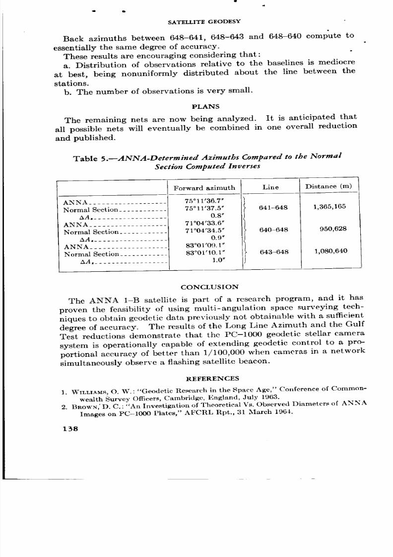
8/7/2019 Significant Achievements in Satellite Geodesy 1958-1964
http://slidepdf.com/reader/full/significant-achievements-in-satellite-geodesy-1958-1964 139/170
SATELLITE GEODESY
Back azimuths between 648-641, 648-643 and 648-640 compute to
essentially the same degree of accuracy.
These results are encouraging considering that:
a. Distribution of observations relative to the baselines is mediocre
at best, being nonuniformly distributed about the line between thestations.
b. The number of observations is very small.
PLANS
The remaining nets are now being analyzed. It is anticipated that
all possible nets will eventually be combined in one overall reduction
and published.
Table 5.--ANNA-Determined Azimuths Compared to the Normal
Section Computed Inverses
ANNA ...................
Normal Section ............
AA, ..................
ANNA .... .. .. .. .. .. .. .. .
Normal Section ............
AA, ..................
ANNA .... .. .. .. .. .. .. .. .
Normal Section ............
AA ...................
Forward azimuth
75°11'36.7 "
75°11'37.5 _
0.8*
71°04'33.6"
71°04'34.5"
0.9 _
83°01 '09.1"
83°01'10.1"
1.0 _
Line
641-648
640-648
643-648
Distance (m)
1,365,165
950,628
1,080,640
CONCLUSION
The ANNA 1-B satellite is part of a research program, and it hasproven the feasibility of using multi-angulation space surveying tech-
niques to obtain geodetic data previously not obtainable with a sufficient
degree of accuracy. The results of the Long Line Azimuth and the Gulf
Test reductions demonstrate that the PC-1000 geodetic stellar camera
system is operationally capable of extending geodetic control to a pro-
portional accuracy of better than 1/100,000 when cameras in a network
simultaneously observe a flashing satellite beacon.
REFERENCES
1. WILLIAMS, O. W.:"Geodetic Research in the Space Age," Conference of Common-
wealth Survey Officers, Cambridge, England, July 1963.
2. BROWN,' D. C. : "An Investigation of Theoretical Vs. Observed Diameters of ANNA
Images on PC-1000 Plates," AFCRL Rpt., 31 March 1964.
138

8/7/2019 Significant Achievements in Satellite Geodesy 1958-1964
http://slidepdf.com/reader/full/significant-achievements-in-satellite-geodesy-1958-1964 140/170
The following paper is excerpted from a report presented atthe lOth International Congress of Photoqrammetry, Lisbon,Portugal, September 1964.
N66 3?35?
SECOR for Satellite Geodesy
T. J. HAYes
Topography and Military Engineering O_ce
Chief of Engineers?
THE SECOR CONCEPT
ECOR IS A_¢ ACRO_+YMformed from the method by which the systemoperates: Sequential Collation of Range. The system is essentially
an electronic distance measuring system designed to make use of the
intermediary space positions of artificial satellites for determining
geodetic positions on earth. The application of the geodetic data that
is collected is based on the trilateration principle whereby three or more
ground stations are placed at surveyed geographical locations of known
geodetic coordinates. These individual locations can be as much as
2300 miles apart, depending on the altitude of the satellite. A fourth
station is placed at some geographic location for which the coordinates
are desired. When the satellite appears above the radio horizon of the
ground stations, each ground station sequentially ranges to the space-
borne satellite on a time-shared basis in exact synchronism as established
by the station selected to be the master timekeeper.
The precise slant range between each of the four stations and the
transponder in the satellite is determined from phase comparisons of
modulations transmitted to and returned from the transponder on radio-
frequency electromagnetic waves. Each station records its range dataon magnetic tape simultaneously with signals from an electronic clock
(accurately set by means of Bureau of Standards timing signals) which
permits fixing the location of the satellite in space. Since several posi-
tions (at least three) of the satellite relative to the ground stations are
then known, the position of the fourth station relative gu Lhe first th._e
stations can be calculated. The recorded data are translated into a
format suitable for use by an electronic computer located at the Army
Map Service. Using basically a space resection computation from satel-
139

8/7/2019 Significant Achievements in Satellite Geodesy 1958-1964
http://slidepdf.com/reader/full/significant-achievements-in-satellite-geodesy-1958-1964 141/170
SATELLITE GEODESY
lite position triangles, the computer calculates the desired geodetic
coordinates independent of the satellite's orbital parameters. The
accuracy of the calculations for the position location is enhanced by the
vast data redundancy provided by the system. For a typical satellite
pass of six minutes duration, for example, the total number of ranges
measured by four ground stations is approximately 29,000. Because of
considerations of geometry it is necessary to collect data during at least
two satellite passes to determine the geodetic position of the unknown
station. In practice, a larger number of passes are used to afford the
best geometry.
The computational procedure is repeated until the required precision
criteria are met. When the unknown station's geodetic coordinates are
considered acceptable, this fourth station can then be designated as a
station of known geographical location. This permits one of the other
stations to leapfrog to another location whose position is desired. Thus,
control will be extended by this progressive method.
EQUIPMENT COMPRISING THE SECOR SYSTEM
The new SECOR system has been developed by the Cubic Corporation
under the guidance of the U.S. Army Engineers. The basic equipment
for operation of the SECOR system consists of at least four identical
ground stations and an earth-orbiting satellite carrying a SECOR
transponder.
SECOR GROUND STATION COMPONENTS
The most complex part of the SECOR system is the ground station
element. Each SECOR ground station consists of three air-transport-
able shelters: The Radio Frequency (RF) Shelter, the Data Handling
(DH) Shelter, and a Storage Shelter. Each ground station also carries
its own support equipment which includes test equipment, generators,
air conditioners, ranging antenna, communications antenna, single side
band communication equipment, and wheel adapters for each shelter.
All shelters and equipment are ruggedized for extensive and varied
field operations.
Major units in the RF Shelter include receivers, transmitters, power
supplies, antenna control assembly, and intercommunications equipment.
Although the antenna is normally mounted on the RF Shelter, it may be
operated from a ground mount if required. After the satellite signal isacquired (usually from prediction data provided to each station ahead
of time) the RF operator tracks the satellite by keeping the antenna
pointed in the direction of maximum signal as shown by signal strength
meters mounted on the antenna control panel.
140

8/7/2019 Significant Achievements in Satellite Geodesy 1958-1964
http://slidepdf.com/reader/full/significant-achievements-in-satellite-geodesy-1958-1964 142/170
SECOR ]FOR SATELLITE GEODESY
The digitizing of the ranging and timing data is accomplished in the
Data Handling (DH) Shelter. The major units in this shelter include
the magnetic tape recorder, quick-look recorders, control console, timing
assembly and master intercommunications. The data handling equip-ment controls the modulation and timing of the pulses transmitted by
the RF equipment and converts the transponder replies into a form suit-
able for recording on magnetic tape. The quick-look recorders, by
presenting a continuous visual plot on moving paper tape, provide the
operator with a constant check of system operation during a pass.
The Storage Shelter contains radio equipment for communication
with the other ground stations and with Field Headquarters. It also
accommodates test equipment and working space for servicing electronic
equipment.
Since the SECOR system is planned for use in a worldwide, leap-
frogging operation to tie continents, geodetic datum, and islands into
one geodetic control net, the ground-based components have been de-
signed to be compatible with several modes of transport. SECOR
ground stations may be air transported by aircraft and helicopter. The
stations also can be carried over water by ship and landed by landing
craft. Overland travel is easily effected by towing.
Each ground station and the satellite transponder comprise an elec-tronic distance measuring unit which is largely automatic in operation.
Distance measurements are made to the satellite-borne transponder by
determining the round-trip phase shift of a series of modulated signals
transmitted by the ground station and retransmitted by the transponder.
The RF signal carrying the modulation frequencies is transmitted by the
ground station to the satellite whose transponder demodulates these
frequencies and retransmits the modulations on two offset carrier fie-
queneies to the ground station. The shift in phase between outgoing
and returned modulation signals is measured and then recorded on
magnetic tape. By measuring the phase delay on several related
modulation frequencies and augmenting these data with the time delay
of a radar-like pulse, unambiguous measurements are obtained. The
two offset carrier frequencies provide correction for ionospheric refraction,
a problem common to all techniques using electronic magnetic waves.
SECOR SPACEBORNE COMPONENTS
The spaeeborne portion of the SECOR system consists of a SECORtransponder whieb may be mounted in its own separable satellite or
installed as an integral part of a larger satellite.
The SECOR transponder is composed of a receiver, transmitters, and
power supply which converts the satellite battery voltage to the voltages
required.
141

8/7/2019 Significant Achievements in Satellite Geodesy 1958-1964
http://slidepdf.com/reader/full/significant-achievements-in-satellite-geodesy-1958-1964 143/170
SATEUITE GEODESY
In operation, the transponder remains in a standby condition until .activated by a select call signal generated by a SECOR ground station.
Upon activation, the transponder receives and retransmits the ranging
frequencies. This sequence is repeated for each ground station in turn,
one complete cycle from the four ground stations occurring every 50
milliseconds. The same ranging and carrier frequencies are used by all
four stations.
SECOR SATELLITE
To at tain a flexible launch capability required to carry out an opera-
tional program, the U.S. Army Engineers developed a self-contained,
separable SECOR satellite that could operate in its own orbit and would
be of a size, shape and weight that would permit the satellite to ride as a
hitchhiker on one of many available boosters. This resulted in thecurrently orbiting Type I1 SECOR satellite. It is 10 in. wide, 13 in.
long, 9 in. high, and weighs about 40 pounds. I n addition to the SECOIt
transponder, the satellite carries solar cells, batteries, a telemetry system,
an antenna system, and a magnetic orientation device.
OPERATING MODES
Figure 1 illustrates the operation of the SECOR system in its tw o
principal modes of operation : simultaneous and orbital. The simulta-
neous mode will be used except when geography forces the use of the
orbital mode.
Figure 1.-Simultaneous and orbital tracking modes.
142

8/7/2019 Significant Achievements in Satellite Geodesy 1958-1964
http://slidepdf.com/reader/full/significant-achievements-in-satellite-geodesy-1958-1964 144/170
SECOR FOR SATELLITE GEODESY
In the simultaneous mode, range measurements are made to the
satellite in rapid sequence (essentially simultaneously) from each of four
ground stations during the period when the satellite is above the radio
horizon of the ground stations. Three of the ground stations are located
at known geodetic positions, and the fourth ground station is positioned
at a site where geodetic coordinates are desired. Range measurements
obtained in the simultaneous mode permit the determination of the
desired geodetic coordinates independent of the satellite's orbital param-eters.
When the geographic locations are such that the satellite can be viewed
simultaneously by the three known stations only, and the unknown
station is able to view the satellite shortly before or after on the same
pass, the orbital mode will be used. In this case an arc of two or more
satellite orbits precisely determined by the three known stations will be
extrapolated over the vicinity of the unknown station. Observed ranges
from the unknown station to satellite positions on the extrapolated
sections permit the desired geodetic coordinates to be established.
The line crossing mode is a special case of the simultaneous mode.
Geography may force the spread of the stations in a less-than-optimum
ground geometry with associated low-look angles and long distances.
The simultaneous solution for the position of the unknown station in the
above case may be strengthened by the direct determination of the
geodetic length of the lines from the unknown station to the three -known
stations by incorporating line crossing techniques. The known stations
accurately determine the height of the satellite at the time when the sum
of the ranges from the unknown station to the satellite and from the
satellite to a known station is a minimum. This provides an additional
mathematical constraint on the geodetic solution.
TESTING THE SECOR SYSTEM
To insure that the SECOR system as developed would fulfill the
requirements of this research and development task, tests were performed
on the various units and subsystems which comprise the system, then
upon the composite system as a whole. Essentially, these tests may be
described as tests of the ground station equipment prior to satellite
launch, tests on the satellite prior to launch, and system tests conducted
both prior to and after launch.
To insure that the satellite would carry out the mission for which it
was designed and developed, it was subjected to a full program of tests
covering all the parameters and conditions considered impori_t_t to
system operation. The results indicated that the satellite would perform
quite favorably within the anticipated launch and space environments.
The satellite tracking phase of this development was planned to eval-
143

8/7/2019 Significant Achievements in Satellite Geodesy 1958-1964
http://slidepdf.com/reader/full/significant-achievements-in-satellite-geodesy-1958-1964 145/170
SATELLITE GEODESY
uate the test data obtained in the different operating modes to enable a .
determination of SECOR system capabilities and thus to minimize the
training, operating, maintenance, and data processing problems inevita-
bly encountered after a new system goes operational. At the time that
the satellite tracking plan was prepared it was envisioned that most ofthe simultaneous mode test data would be obtained on a small (500-mile)
quad, with ground stations based at Stillwater, Oklahoma; Las Cruces,
New Mexico; Austin, Texas; and (the unknown site) Fort Carson,
Colorado, and that the orbital mode test data would be acquired utilizing
the small quad plus the station located at East Grand Forks, Minnesota.
Orbital mode operations were conducted for a period of about three
weeks on the small quad with the East Grand Forks station. The track-
ing data were obtained in such a manner that the data could be evaluated
in both the simultaneous and orbital modes of operation. The results ofsimultaneous data reduction were used to check the results of orbital
data reduction, clearly indicating where the orbital data reduction was
erroneous. This comparison was necessary due to the unprecedented
accuracy required in the projection of the satellite trajectory.
It is believed at this time that reduced accuracy in the orbital mode
accrues from three primary sources; namely,
(1) Relatively small orbit fitting spans.
(2) System errors.
(3) Base site survey errors.
(4) Internal timing errors.
Small fitting spans allow any error in the data to upset the vector
fitting and give less accuracy in the injection vector determination; the
forward prediction then deterioratcs rapidly. System and survey biases
give a slight misorientation of the injection vectors and, therefore, affect
the forward predictions also. Timing error arises from lack of exact
synchronization of clocks at the ground stations, and any time offset will
mean that the predicted satellite positions and the measured ranges will
not be coincident. Time synchronization problems are not encountered
when the Geodetic SECOR equipment is used in the simultaneous mode.
The station at Las Cruces, New Mexico, was then moved to Larson
Air Force Base, Washington, to complete the large quad shown in Figure
2. The longer ranges and lower elevation angles to the satellite obtained
on this quad provide the difficult operating conditions more typical of
those likely to be met in operational usage. Data obtained in the simul-taneous mode on this quad were also reduced and evaluated in the orbital
and line crossing modes to compare the capabilities and limitations of
each mode for given satellite/ground station geometries, etc.
144

8/7/2019 Significant Achievements in Satellite Geodesy 1958-1964
http://slidepdf.com/reader/full/significant-achievements-in-satellite-geodesy-1958-1964 146/170
SECOR FOR SATIR.I.ITE GEODESY
/ , a-li.LARS0NJ---____/ _- #/* ....... /;'" :_ I
/ ....,. _ : Z """t..... ' ...... !.. i E GRAND FORKS I _, )-._S_Jl;'. ; . i_ ,' ' _ --'r :" .-...-- ._ _I.-? t../i
• . 7-.- I ' -\ _,i-4 ) ' - _ _ -"1_, \_ -._'_- _ _ ...._.... .-. , ,,__'_;,_...._._ _\- ,i
iN._-\' t, --r-'-i-__! %1"*'...... "-_2--_ \ tl.... I - _ i- - _v-- - _ .....ilk_SAN DIEGO............ _---- _ \ I
- / "C"<. , , " I _.°...... I........ J,. -- -- <-'-k -%.%/ \ II
7 ":'7 All
SIM LANEO SO'E /L
-_'_ / f ...... --,L.... V._. I _- t ,'tf_--,
'7,.. ; " , ,' " ,......_..._ ,/_<.L.!_- / L;?:_ h"0.... --- _ " -)'7---r---f---_ - t)_--<_ t-C.4V
"4 - _ - - " /1 I ..... l..... i" .,-...l....*gr'._\/_.._ _._S_'\(_'_ _--_I ...... _-/-- i-'--_t it, ._'3_:L"r2j,.-_t
,t \ _-._ , i__ _ _ .... _' ___'; \,/'. \\ C it ..... FT. CARSON_HERNDONqI_" \
¢-- ......... g,,",, ,ill. SAN DIEGO...... I , ........ , .... . z_,- =. <. \
/ i-"---k--L__'_ "'--"--,---_--_ ! --_ !:_ .......x.......,,t \
• i RU_/III_ ' '
It/ ct, .IJ/ TYPICAL LINE CROSSING MODEti _ I 1 i ,' ' I , I
Figure 2.--Expanded test phase.
In the large quad data reduction, Larson Air Force Base, Washington,
was the unknown station.
[Table 1 lists the majority of the unknown station soIutions
processed for the large quad. SECOR survey differences result
145

8/7/2019 Significant Achievements in Satellite Geodesy 1958-1964
http://slidepdf.com/reader/full/significant-achievements-in-satellite-geodesy-1958-1964 147/170
SATELLITE GEODESY
from averaging a sequence of actual Geodetic SECOR solutions
and subtracting the U.S. Coast and Geodetic Survey site coordinates
from this average solution. The standard deviations shown per
solution are computed from the residuals which are the differences
between each SECOR-survey offset and the average of the offsetsfor one particular solution. RSS refers to "root sum square" and
indicates composite bias and noise error. The RSS is computed by
squaring the mean offset and the standard deviations, adding and
taking the square root of the sum.]
Utilizing generally the same line crossing technique currently employed
by systems such as HIRAN (but in this case employing the satellite as a
super-elevated spaceborne station in place of the HIRAN airborne
station), line crossings were initiated on a comparatively short line (1150
miles) between San Diego, California, and Stillwater, Oklahoma, for a
period of about one week to resolve operational problems, determine the
accuracy obtainable with the line crossing technique, and finalize the
computer program. Geometry was selected to allow good satellite
altitude determination by data obtained from three of the four stations
on the small quad. Data from the line crossings then were used to
determine satellite position and geodetic distances between San Diego
and Stillwater.Line crossing operations were then switched to a long line (2300 miles)
between San Diego and Herndon, Virginia, for a period of about three
weeks to determine the ultimate operational and accuracy limitations of
the SECOR system for line crossing operations. Measurement errors
from tropospheric refraction, ionospheric refraction, and multipath effects
increase as elevation look angles are decreased. The data gathered
should determine the accuracy of SECOR measurements at the long
ranges obtainable when using satellites for line crossings.
Table 2 contains a summary of the line crossing solutions and com-
parisons computed from tile satellite data. The results of the line cross-
ing mode are commensurate with the theoretical results with the exception
that all but 2 of 17 lines measured to the Herndon, Virginia, site are
longer than the inverse lengths.
The line crossing solution in this experiment is made possible by the
use of ground stations to track the satellite during the crossing. The
line crossings processed here represent the longest lines ever measured
and clearly demonstrate the potentiality of the technique.A simulation study was performed by the contractor, Cubic Corpora-
tion, to aid in the evaluation of the different operational modes (simul-
taneous, orbital and line crossing). Effects of base site geometry, errors
in site survey, tropospheric and ionospheric refraction, scale factor, and
146

8/7/2019 Significant Achievements in Satellite Geodesy 1958-1964
http://slidepdf.com/reader/full/significant-achievements-in-satellite-geodesy-1958-1964 148/170
{D
SECOR FOR SATELLITE GEODESY
v_9
_6
l
_ 77777 _ 777 7
I
0_
"S__-_._
II II
147

8/7/2019 Significant Achievements in Satellite Geodesy 1958-1964
http://slidepdf.com/reader/full/significant-achievements-in-satellite-geodesy-1958-1964 149/170
N
SATELLITE GEODESY
L
©
¢)
e'_
_z
e_
Oq
i tt ii i
i i
i
o0
oq
e_
oq
o_
i
i
i i
i
o_
oq
e_
e4
i
i
o0
oq
m.
o_
I '
I
I°
e4
I
o_
oO
i i
J
i i
i
i
O
O
O
oo
oo
i i
i i
i i
i ii
I
O
o4
oo_
i i
i ii i
i
ii
oo
O
o4
i i
i
i
148

8/7/2019 Significant Achievements in Satellite Geodesy 1958-1964
http://slidepdf.com/reader/full/significant-achievements-in-satellite-geodesy-1958-1964 150/170
SECOR FOR SATELLITE GEODESY
qD _ ¢_ OO
_=_
C'q
n_
i i
L i
i
iRi
i
c_
i :
c_
: I
c4
O
r.= r_ co r_.
oo
06
c_
I
¢D
ke_
t_
I If I
L IK II It I
r II I
i
i
i
c_
°
iat
i
d_D
L i
t t
i i
t
_4
c,i
i t
i i
i i
i ti i
i i
_d
tt
_4c_
c,i
o0
_4
i
_d
i
,,-,t
i
i
i
-4 :
it
ii
iii
i
ii
r
i ti ii ii i
i i
i ii i
i ii ii ii Ii ,
l ii i
1 i1 ii ii i
i i
l i
i ii iLi i
i
II
|b
H
b
II
II
0
v
149

8/7/2019 Significant Achievements in Satellite Geodesy 1958-1964
http://slidepdf.com/reader/full/significant-achievements-in-satellite-geodesy-1958-1964 151/170
SATELLITE GEODESY
equipment limitations have been considered with respect to their'effect .
on solution accuracy. In the computer simulation, geometries were
selected to correspond to the actual site locations used in satellite tracking
tests.
LINE CROSSING ERROR ANALYSIS
The method employed to obtain geodetic line crossings from Geodetic
SECOR ranging data is not directly analogous in computational tech-
nique or operational procedure to that performed with HIRAN or
SHIRAN observational data. A distinctly different approach is neces-
sary because the path of the satellite is not essentially concentric with
the earth's surface. The occurrence of a minimum range sum derived
simultaneously from two tracking sites will, therefore, not be coincident
in time with the minimum geodetic line crossing. However, if the range
240
200
160
12ou_
8O
40
0
0
CSys
9'
150
//
CS' _T = 75' / /_s' _T = 60'
N
"s' _ \
10 20 30 40 50 60 70
Elevation angle °
_Tropo alono _Scale _Target _Site
O. 05 O. 05 I ppm Variab le Variabl e
Figure 3.--Geodetic distance error vs. elevation angle.

8/7/2019 Significant Achievements in Satellite Geodesy 1958-1964
http://slidepdf.com/reader/full/significant-achievements-in-satellite-geodesy-1958-1964 152/170
SECOR FOR SATELLI'I_E GEODESY
obsel:vations are projected onto the earth's surface at each point along
the satellite's orbit, then the sum of the geodetic distances from two sites
4o the subtrace of the satellite will have a minimum coincidently and
approximately equal to the minimum distance between the two tracking
sites.
In the modified version of the classic HIRAN-SHIRAN line crossing
schemes, it is assumed that the heights above mean sea level of the end
points of a line are known. It has also been assumed that the geocentric
coordinates of the vehicle will be known too, either by direct solutionfrom three simultaneously-tracking known base sites or by orbital pre-
dictions. The distance of the satellite from earth center is computed
from the geocentric coordinates. With the station heights, satellite to
earth center distance, and approximate knowledge of the geodetic coordi-
nates of the end points of a line, the projections onto the reference sphe-
roid of the range measurements to each site can be computed. The
minimum geodetic distance is now computed from the composite set of
adjacent projections.In the error analysis for the geodetic satellite line crossing, the effects
of three major factors on the geodetic distance computation are evalu-
ated; namely,
(1) Ranging errors due to sources such as refraction, scaling, system,
etc.
(2) Station height errors, which are errors in independent height-
above-mean-sea-level measurements.
(3) Vehicle height errors, or errors in earth center to satellite distance.
Table 3.--Relative Contribution of Error Sources to Geodetic Line
Crossing Error
Elevation Vehicle Stationangle Total RSS height Ranging height
lO°.......20 ° ........
30 ° ........
40 ° ........
50 ° ........
60 ° ........
70"- .......
18.3'
17.7
19.8
24.0
30.8
44.0
64.0
7.7'
9.1
11.3
14.5
19.0
26.0
40.5
16.3'
14.2
13.8
14.7
16.6
21.4
29.3
2.6'
5.5
8.6
12.5
17.6
25.0
40.0
Error Mode/
9 t
OTro_
0.05
_Iono
0.05
_r_e
1 ppm
_r Target
15'
O'Site
15'
151

8/7/2019 Significant Achievements in Satellite Geodesy 1958-1964
http://slidepdf.com/reader/full/significant-achievements-in-satellite-geodesy-1958-1964 153/170
SATELLITE GEODESY
A set of geodetic distance versus elevation angle error curves' were
processed using a composite typical error model and different station and
vehicle height errors. Figure 3 illustrates these error propagations.,
Table 3 shows the amount each major error source contributed to the
total geodetic distance error for one case shown on Figure 3. A satellite
height of approximately 500 NM was used in this propagation.
The line crossing analysis demonstrates that ranging accuracy controls
the geodetic distance error propagation at low elevation angles. When
elevation angles exceed 30 ° , station height and vehicle height errors pre-
dominate. In all cases, solutions should be constrained to lines with
elevation angles less than 45 ° .
All errors propagated in this evaluation are carried as random and un-
correlated errors. The results are therefore conservative. In actualsolutions, and in particular under the scheme used to compute the satel-
lite geodetic line crossing, errors will be correlated and will give either
equal or more accurate results.
CONCLUSION
The advent of artificial satellites has opened doors to technological
advances that were only dreams less than a decade ago. In January
1964 a United States Army Corps of Engineers artificial satellite carryinga SECOR transponder successfully achieved orbit. This event made
possible a series of tests of this new geodetic electronic ranging system.
The tests, which were completed on 1 May 1964, clearly established that
the SECOR system has the full capability of a first order geodetic tool.
152
8/7/2019 Significant Achievements in Satellite Geodesy 1958-1964
http://slidepdf.com/reader/full/significant-achievements-in-satellite-geodesy-1958-1964 154/170
Part 6
Summary and Conclusions

8/7/2019 Significant Achievements in Satellite Geodesy 1958-1964
http://slidepdf.com/reader/full/significant-achievements-in-satellite-geodesy-1958-1964 155/170
' Nor
Summary and Conclusions
ATELLITE GEODESY is conveniently considered as dividedinto gravitational or dynamical geodesy and geometrical
geodesy; in practice, of course, there is some overlap.
Dynamical geodesy comprises the study of the Earth's
gravitational field through the use of satellites as in situ probes.
The techniques employed are the traditional techniques ofcelestial mechanics modified and updated to apply to close-
Earth satellites in the presence of a perturbing nonspherical
Earth, the Moon, and the Sun, and particularly adapted to
rapid calculation with modern high-speed electronic com-
puters.
Starting with the determination of the improved value of
the flattening of the Earth in 1958, this field has matured
until, in the past 18 months, consistent values have been de-
rived for a number of zonal and tesseral harmonics by several
analysis techniques and from several types of data. The
lower terms, which are best determined, are summarized in
the following table for the zonal harmonics, and in the table of
tesseral harmonics (Pt. 3, paper by Wagner). By contrast,
only the flattening value was well established before the
Zonal Harmonics
Ka_la Kozai Anderle
J2 1082.20X 10 "_ 1082.63X10 _ 1082.65X10 _
J3 -2.57 -2.56 -2.59
J4 -2.01 - 1.63 - 1.53
J5 -0.066 -0.185 -0.165
J6 +0.324 +0.593 +0.793
J7 -0.465 -0.376 -0.426
155

8/7/2019 Significant Achievements in Satellite Geodesy 1958-1964
http://slidepdf.com/reader/full/significant-achievements-in-satellite-geodesy-1958-1964 156/170
SATELLITE GEODESY
satellite era and, as was mentioned above, this proved to be
significantly in error. Additional satellites in a variety of orbit_
will be needed before the dynamical analysis of the Earth's
gravity field reaches the point of diminishing returns, andparticularly before we understand major differences between
terms derived by diverse methods. However, the quality of
the data is already good enough to stimulate geophysical
interpretations and attempts to correlate the satellite results
with surface measurements.
Geometrical satellite geodesy, that is, the use of satellites
as reference points for determining precisely the relative loca-
tions of various points on the surface of the Earth and partic-
ularly for interconnecting datums and placing all observing
stations and all individual datums on a common Earth-
centered reference system, is in its infancy. Analyses of the
Baker-Nunn observations of various satellites by reflected
light, simultaneous photographs of the Echo satellite from
widely separated portions of the Earth, analyses of Doppler
data by various TRANET stations and analyses of the ranging
data obtained using the SECOR system have all indicated
that we are on the verge of significant progress in the area of
geometric geodesy, but it will probably be at least 5 years
before such observations contribute in a major way to map-
making. Not only will placing the entire world on the same
coordinate system be useful to geographers and navigators
but it will also aid in space-probe tracking and in geophysics.At present, observations from various stations in NASA's deep
space net cannot be combined without introducing an addi-
tional error from the uncertainty in the relative coordinates
of the various stations. World gravity observations also lose
some of their value because of the difficulty in interconnecting
observing sites accurately. The geodetic satellite p/ogram
should signficantly improve this situation.
The launch of Geos in 1965 into an orbit specifically selected
for dynamical geodesy should contribute appreciably to both
geometrical and dynamical geodesy. Geos will carry a
flashing light, a Doppler transmitter, two ranging systems,
156

8/7/2019 Significant Achievements in Satellite Geodesy 1958-1964
http://slidepdf.com/reader/full/significant-achievements-in-satellite-geodesy-1958-1964 157/170
SUMMARY AND CONCI.USIONS
and corner reflectors for use with laser transmitters. The
_ranging systems and the laser reflections, if the latter prove to
be a satisfactory operational system, should greatly improve
the determination of scale--a major problem in geometrical
geodesy. The launch of the Pageos satellite, an Echo-type
balloon, in a 3000-km orbit will provide an excellent target
for triangulation across intercontinental distances and can
serve as a basis for a worldwide geodetic network. Finally,
for a detailed understanding of the mass distribution in the
outer regions of the Earth, the gravitational field derived
from satellite observations must be combined with local
measurements. An appreciable extension of ground-based
gravity surveys will be needed for this purpose, an extension
which undoubtedly lies outside of the field of satellite geodesy.
On a broader scale, both satellites and probes have given
us better values of the various constants needed to compute
ephemerides for astronomical bodies. The newly adopted
values are given in appendix B. The selection and use of
these values is discussed in Part 4. As the tracking of inter-
planetary probes improves and as lunar and then planetary
orbiters become operational, our knowledge of the shapes,
masses, and gravity fields of the Moon, Venus, and Mars
should be well established. This will, in addition to providing
information on the present structure of these bodies, provide
important boundary conditions for theories of the origin ofthe solar system.
157

8/7/2019 Significant Achievements in Satellite Geodesy 1958-1964
http://slidepdf.com/reader/full/significant-achievements-in-satellite-geodesy-1958-1964 158/170
ot
l_E_'-'-_i_a PAGE BLANK NOT FIL_,ED.
Appendix A
A Review oJ Geodetic Parameters
WXLLI^M M. KAULA

8/7/2019 Significant Achievements in Satellite Geodesy 1958-1964
http://slidepdf.com/reader/full/significant-achievements-in-satellite-geodesy-1958-1964 159/170
The following paper was presented at the International
Astronomical Union Symposium No. 21, "The System of
Astronomical Constants," Paris, May 27-31, 1963.
N66 3?358A Review of Geodetic Parameters
WILLIAM M. KAULA
Goddard Space Flight Center, NASA
SUMMARY
r IS RECOMMENDED that the parametric values which are cur-
rently most used in orbital computation be adopted as
provisional standards, rather than those which may be the best
available, because the "most used" values differ only slightly from
the "best" values and further improvements in the values are
expected within the next 4 years. Some of these values are:
GM_ = 3.986032 X 10²° cm 3 sec -2,
J2 = 1082.30 X 10 -6,
Js = - 2.3 X 10 -_,
J, = - 1.8 X 10⁻⁴,
a, =6,378,165.0 m.
With parameters such as the foregoing the most serious geodetic
errors affecting astronomy are tracking station positions.
Standard methods of describing and transforming positions
are suggested.
INTRODUCTION
This review recommends which geodetic parameters should be adopted
as standard, the manner in which the parameters should be expressed,
and the values which should be adopted. In making these recommenda-
tions, current practice, available determinations, and anticipated im-
provements will be considered.
GRAVITATIONAL PARAMETERS
For the notation of the earth potential, recommendations have already
beeu made by Commi_ion 7 o, C_.lestial Mechanics, of the International
Astronomical Union (Reference 1):
U= u- 1+ " R " p. (sin 3) C.,. cos m)tq-S.,., sin mX (1)r n-i
161

8/7/2019 Significant Achievements in Satellite Geodesy 1958-1964
http://slidepdf.com/reader/full/significant-achievements-in-satellite-geodesy-1958-1964 160/170
SATELLITE GEODESY
where u=GM$, r is the distance from the center of the earth, R is "the
mean equatorial radius of the earth, Pnm is the associated Legendre poly-
nomial, 3 is the latitude, and ), is the longitude. Alternative notations
recommended for the gravitational coefficients are
Jn = - C,.o. (2)
and
[.(n-m). (C_.,_,Sn.,_). (3)
These two additions are suggested:
1. Define
(2n+l) (2-_,_ 0) (C.... Sn.,_), (4)
where the Dirae delta _m° is 1 for m=0 and 0 for m_0. The C .... Sn.,_
are eoeffieients of harmonies which have a mean square amplitude of 1
for all values of n and m.
2. Define the mean equatorial radius more precisely as the equatorial
radius of the mean earth ellipsoid, i.e., the ellipsoid of revolution which
best fits the geoid. This definition is consistent with geodetic practice
and involves the equatorial radius with only two of the set of orthogonal
parameters defining the radius veetor of the geoid--the zeroth and second
degree zonal harmonies. (The more literal definition of the mean equa-
torial radius as the radius of the circle which best fits an equatorial section
through the geoid would connect the radius to the infinite set of even
degree zonal harmonies.) An alternative possibility for the equatorial
radius in Equation 1 is the mean radius of the entire earth which, since it
differs by a factor of 10 -3, would affect the value of J_. The mean radius
seems slightly preferable aesthetieally, but current practice overwhelm-ingly favors the equatorial radius ; a perusal of some papers on close satel-
lite dynamics and orbit analysis found ten workers using the equatorial
radius but none using the mean radius (in addition, five theoretieians did
not define their radius).
To be consistent with the connection of equatorial radius to the mean
earth ellipsoid, it is recommended that the following be the relationships
between the astronomical parameters _=GM_ and J2=-C2.o and the
geodetic parameters R=ae, the equatorial radius; %, the equatorial
gravity; f, the flattening; and _, the rate of the earth's rotation with
respect to inertial space (References 2, 3, and 4) :
GM_=ae2"y,[ l _ 3 m-f --_ mf -_15l mj__O(f4)] ' (5)
162

8/7/2019 Significant Achievements in Satellite Geodesy 1958-1964
http://slidepdf.com/reader/full/significant-achievements-in-satellite-geodesy-1958-1964 161/170
° where
APPENDIX A--REVIEW OF G_ODETIC P_S
2 1 1 3 2 9 2 11 (6)
rn= _'a----_" (7)%
The values of GM¢ and J_ which are probably the most extensively used
at orbit computation centers in the United States are (References 5, 6,
and 7) :
GM¢ = 3.986032 ± 0.000030 X 10 _ cm* see -2, / (8)
J2-1082.30 X 10 -6. !
In the alternative notation of Herrick, Baker, and Hilton (Reference 8)
and Makemson, Baker, and Westrom (Reference 9):
ke-- (GM¢) 1/_= 0.019965049 megameter sn sec -1. (9)
The values of GM_ and J2 in Equation 8 are consistent with thesevalues for the geodetic parameters:
a,=6,378,165.0+_25.0 meters, t
3,,=978.0300±0.012 cm see -2, (10)
f= 1/298.30,
to= O.729211585 X 10-4 sec-1.
The value for a, is a compromise between the solutions of Fischer (Refer-
ence 10), and Kaula (Reference 11), and other values which are unpub-
lished. The 3,, value differs from that of the International Formula and
the Potsdam System (978.0490 cm sec -_) in three ways:
1. Correction to Potsdam System absolute g (Reference 12)=
- 0.0128 + 0.0003;
2. Change of flattening from 1/297 to 1/298.3 =--0.0051;
3. Change of mean gravity over the earth's surface (Reference 11)=-0.0005+0.0012.
The correction to absolute g is a provisional value and has not been
___.opf_l by the International Union of Geodesy and Geophysics; an
improved value should be forthcoming within the next Iew years from
several determinations in progress (Reference 13). The correction to
mean gravity is negative, mainly because correlation between gravity
and topography was used to estimate anomalies for the areas without
163

8/7/2019 Significant Achievements in Satellite Geodesy 1958-1964
http://slidepdf.com/reader/full/significant-achievements-in-satellite-geodesy-1958-1964 162/170
I SATELLITE GEODESY
observations, which are predominantly oceans. Solutions by U_)tila
which fit observed gravimetry and do not use correlation with topography
give positive corrections ranging from q-0.0004 to -b0.0019 cm sec -_.
(Reference 14). Rather slow improvement is expected; problems in
observing gravity at sea are not entirely solved (References 15 and 16).
Some improvement may also come from using the better statistical
techniques which larger capacity computers permit.
The value of GM¢ may also be obtained through the modified Kepler
equation by using the radar mean distance of the moon A and the moon's
mean motion n:
n 2 (1 -_-_) aGM_=-- A 3, (11)
l+h_
where 3 is the solar perturbation of the mean semirriajor axis and PM/_E
is the ratio of the moon's mass to the earth's mass, equal to the lunar
inequality (Reference 17). The most recently published value for A is
384,402.0+1.2 km (Reference 18). As pointed out by Fischer, this
value should perhaps be corrected because it is dependent on an exces-
sively rounded-off lunar radius of 1740 km (Reference 19). The mean
radius of the lunar limb is 1737.85_+0.07 km. Geometrical determina-
tions of the radius toward the earth vary considerably; Baldwin's
conclusion (Reference 20) leads to 1740.05 kin, whereas Schrutka-
Rechtenstamm (Reference 21) concludes that the bulge is too small to
be determined. However, we are not interested in just the long axis of
a best-fitting triaxial ellipsoid, but rather in the mean radius of the area
contributing to the leading edge of the radar return pulse, which would
fall within the _+7 degree area of libration. Contour maps of the moon
(Reference 22, for example) indicate that the average radius of this _7
degree area could differ by as much as 2 km from the best-fitting ellipsoid.
If the lunar surface is assumed to be an equipotential surface, then usingthe moments of inertia obtained from the physical libration yields
1738.57 km as the radius toward the earth. Letting A =384,400.5_+ 1.2
kin, 3=0.0090678, n=2.6616997X10 -B sec -1 (Reference 23), and
UM/_ = 1/(81.375_+ 0.026) (Reference 24) gives
GM$ ---3.986094 _+0.00004 X 10 _° cm 3 see -2. (12)
Using the _M/_E= 1/81.219 of Delano (Reference 25) reduces GM$ to
3.986001X10²° cm 3 sec -2, so the difference from solutions based on
terrestrial data seems largely explicable as an error in the lunar inequality.
The larger computers of today permit the application of more elaborate
statistical techniques than it was possible to apply in 1950 (the year
Delano and Rabe published their work). However, since the stellar
164

8/7/2019 Significant Achievements in Satellite Geodesy 1958-1964
http://slidepdf.com/reader/full/significant-achievements-in-satellite-geodesy-1958-1964 163/170
APPENDIX A_REVIEW OF GEODETIC PARAMETERS
positions are a major suspect for systematic error, it seems premature to
reanalyze the Eros observations before the revised reference star systems
•are available (Reference 26). Meanwhile, improved determination of
the lunar inequality may be obtained from radio tracking of space
probes such as Mariner II (1962 apl). Also, since spacecraft have been
launched into high, nearly circular orbits such as those of Midas III
(1961 a) and Midas IV (1961 a$), it may be worthwhile to try to
determine GMe from close satellite orbits.
In addition to GMe and J2, standard orbit computation programs
usually incorporate J8 and J4. The values which are probably most
common at United States computation centers are (Reference 6) :
Ja = - 2.3 X 10-e,
J4 = - 1-8X 10-_-_} (13)
At present the best values of the zonal harmonics are undoubtedly those .....
of Kozai (Reference 7) :
J_= 1082"48+0"06)<10-6' J:= -2"562-+ 0"012X 10-e "1
J4 = - 1.84_+0.08X10 -s, Js-- -0"064+0"019X10-e t (14)s = 0.39 __+.12 X 10 -6 , J7 = - 0.470 + 0.021 × 10-e,
Js= -0.02_+0.02)<10 -6, Ja=0.117__+0.025X10 -6. J
Note that the J2, J:, and J4 now used, given in Equations 8 and 13, each
differ from Kozai's improved values by less than 0.3)< 10-6; and that the
coefficients J5 and higher are all very small in absolute magnitude.Therefore, it does not seem worthwhile to adopt values, other than
those already in general use, before 1966 or 1967, when analysis of
geodetic satellite orbits observed during the International Year of the
Quiet Sun will be completed.
Most of the current close satellite orbit analyses for geodetic purposes
seek tesseral harmonic perturbations. In view of the smallness of these
perturbations, it does not seem appropriate to adopt standardized values
for the tesseral harmonics C .... S_._. The one exception might be
C2.2, S_.2, for which an upper limit would be useful because of its effect
on supplemental energy requirements for 24 hour orbits. The most
recent, unpublished determinations of Izsak, Kaula, Kozai, and Newton
range from 0.9)< 10 -6 to 1.8)< 10 -_ in amplitude (%/C2f-4-S_.2 _) and from
8_"to 25_ W in _ne...._AIDt_CI_IOa'... Ole ,'L. _ --..: '_ ^'__1bliV pliav,.Lpa, a.,_" L_,.L/[I'I/9_÷a'n-?,{.q,,/,-- ,_-.,,-/e:.._l_,-. _-
GEOMETRICAL PARAMETERS
As shown by analyses involving large systems of observations (Refer-
ences 10, 11, and 19), the equatorial radius is a derived, rather than a
165

8/7/2019 Significant Achievements in Satellite Geodesy 1958-1964
http://slidepdf.com/reader/full/significant-achievements-in-satellite-geodesy-1958-1964 164/170
SATELLITE GEODESY
fundamental, quantity: accurate knowledge of the radius is not necessary
to obtain other parameters, such as the lunar distance, geoid undulations,
or datum positions by fitting of the astro-geodetic to the gravimetric,
geoid. However, for astronomical purposes, it is desirable to have a
reference ellipsoid correct within _+50 meters in order to obtain reason-
ably correct positions of isolated tracking stations from astronomic
latitude and longitude. Also it is convenient to have a unit of length
approximating the earth's radius for use in the potential formula (Equa-
tion 1) and for use as a base line to compare or combine parallax observa-
tions. For these astronomical purposes, the value of 6,378,165.0 meters
given in Equation 10 should be entirely adequate. Marked improve-
ment is not expected for about 5 years, by which time satellite observa-
tions should contribute significantly to the strengthening of triangulationsystems and to the interconnection of geodetic datums.
By far the most annoying problems in the astronomical application of
geodetic data pertain to tracking station positions. Errors in the
adopted values of station positions, in conjunction with drag and non-
uniform distribution of observations, prevent accurate determination of
tesseral harmonics and are even believed to be a major cause of discrep-
ancies in space probe trajectories (Reference 27). These station position
errors are due to both inadequate data and mistaken treatment of data;
in descending order of reprehensibility they include:
1. Weak, erroneous, or nonexistent connection of tracking stations to
local geodetic control (this includes the moving of antennas by stations
without informing the computing center) ;
2. Failure to state the datum or ellipsoid to which tracking station
positions refer;
3. Use of obsolete or erroneous standard datum and ellipsoid;
4. An incomplete or ambiguous statement about how datum or
ellipsoid transformations were made;
5. Failure to provide for geoid-ellipsoid difference in calculating heights;
6. Neglecting systematic error due to incorrect observation (for
example, no Laplace stations) or incorrect adjustment (for example,
arbitrary scale changes or rotations) of geodetic control connecting
tracking stations more than, say, 1000 km apart ;
7. Actual observational error of position.
In view of the number of geodetic datums and corrections thereto, they
do not seem to be appropriate parameters to be adopted as standard by
an international organization, except possibly for the large continental
triangulation systems. The corrections to coordinates u, v, w with posi-
tive axes directed respectively toward latitude and longitude (0 °, 0°),
(0 °, 90 ° E), (90 ° N) obtained in the world geodetic system solution of
166

8/7/2019 Significant Achievements in Satellite Geodesy 1958-1964
http://slidepdf.com/reader/full/significant-achievements-in-satellite-geodesy-1958-1964 165/170
APPDOIX--mEvx_r GEOD_"nCPaX,_'_S
Table 1.---_rrections to u, v, w From Re]erence 11 (Meters)
Datum shift Au _v Am
WGS-NAD ........... --23±26 +142__+22 +196+22
WGS-ED ............. -57+_23 --37_+29 --96_+23
WGS-TD ............. -89 +_40 +551 _+53 +710 _+40
Kaula (Reference 11) are listed in Table 1, where NAD, ED,,.and TD
refer to the North American, European, and Tokyo datums, respectively.
The uncertainties in this table are based on estimates of the errors due
to interpolation and representation in the astro-geodetic and gravimetrie
geoids, and are probably a fair measure of item 7 on the above list, but
may neglect significant effects falling under item 6. The relationships of
the rectangular coordinates u, v, w to the geodetic latitude ¢, longitude X,
and elevation h, referred to an ellipsoid of parameters a, and f, are:
u=O,+h) cost, cos X, /
v= (r+h) cos _ sin X, /
w=[(1--e a) v+h] sin ¢,l
(15)
where r = a,/(1-- e_ sin __),n and ea = 2f--fL
To help minimize the number of unnecessary errors in categories 1
through 5 on the above list, it is suggested that organizations be urged
to publish the following information pertaining to each tracking station
for which they publish any precise observations of artificial satellites or
probes, or orbital data based thereon:
1. The names and coordinates of local geodetic control points, both
horizontal and vertical, to which the tracking station is connected;
2. The geodetic datum and ellipsoid to which the horizontal coordinates
refer;
3. The organization which established the local geodetic control points;
4. The manner in which the horizontal and vertical survey eonnections
were made from the local control points to the tracking station;5. The date of the survey connection and a description of the termina-
tion point of the survey;
6. The geodetic (¢, X, h) and rectangular (u, v, w) coordinates of the
-*_-'^- mfc...ve_._ ,. ,h_ lew-_lmwtotie, datum:
7. A statement of the geoid height, if any, estimated for the station
and the basis for the estimate;
8. If the tracking station position has been shifted for the purpose of
referring observations (direction cosines or altitude and azimuth) or
167

8/7/2019 Significant Achievements in Satellite Geodesy 1958-1964
http://slidepdf.com/reader/full/significant-achievements-in-satellite-geodesy-1958-1964 166/170
SATELLITE GEODESY
calculating orbits, the geodetic and rectangular coordinates after the
shift and the ellipsoid to which the new coordinates refer.
Every item on this list is an action which must be accomplished fo_
any tracking station, but thus far the Smithsonian Astrophysical Institute
Baker-Nunn camera network is the only one for which even part of the
list has been published (Reference 28). It is symptomatic of the diffi-
culties which occur that, since this publication, the coordinates for at
least four of the twelve Baker-Nunn cameras have been found to be in
error by 20 meters or more. These geometrical details of tracking station
position are rather uninteresting, but they must be examined carefully
and determined correctly if the full potentialities of modem tracking
techniques are to be realized.
REFERENCES
1. HAGIHABA, Y. : Recommendations on Notation of the Earth Potential. Astronom.
J. 67(1): 108, February 1962.
2. LAMnERT, W. D. : The Gravity Field of an Ellipsoid of Revolution as a Level Sur-
face. Annales Academiae Scientiarum Fennicae, Ser. A-III, No. 57, 1961;
Reprinted in Ohio State Univ., Inst. of Geodesy, Photogrammetry and Car-
tography, Publ. No. 14, 1961.
3. COOK, A. H. : The External Gravity Field of a Rotating Spheroid to the Order of
e8. Geophys. J. 2(3): 199-214, September 1959.
4. HIRVONEN, R. A.: New Theory of the Gravimetric Geodesy. Annales AeademiaeScientiarum Fennicae, Ser. A-III, No. 56, 1960; Reprinted in Ohio State Univ.,
Inst. of Geodesy, Photogrammetry and Cartography, Publ. No. 9, 1960.
5. KAVLA, W. M.: Tesseral Harmonics of the Gravitational Field and Geodetic
Datum Shifts Derived from Camera Observations of Satellites. J. Geophys.
Res. 68(2): 473-484, January 15, 1963.
6. CLARKE, V. C.: Constants and Related Data Used in Trajectory Calculations at
the Jet Propulsion Laboratory. Calif. Inst. Teeh., Jet Propulsion Lab., Tech.
Rept. 32-273, May I, 1962.
7. KozAI, Y.: Numerical Results from Orbits. Smithsonian Inst., Astrophys.
.Observ. Spec. Rept. No. 101, July 31, 1962.
8. HERRICK, S.; BAKER, R. M. L., JR.; AND HILTON, C. G.: Gravitational and Re-
lated Constants for Accurate Space Navigation. In: Proc. 8th Internat.
Astronaut. Cong., Barcelona, 1957, ed. by F. Hecht, Vienna: Springer-Verlag,
1958, pp. 197-235.
9. MAKEMSON, M. W.; BAKER, R. M. L., JR.; AND WESTROM, G. B.: Analysisand
Standardization of Astrodynamic Constants. J. Astronaut. Sci. 8(1): 1-13,
Spring 1961.
10. FISCHER, I.: An Astrogeodetic World Datum from Geoidal Heights Based on the
Flattening f=1/298.3. J. Geophys. Res. 65(7): 2067-2076, July 1960.
11. KAVLA, W. M. : A Geoid and World Geodetic System Based on a Combination of
Gravimetric, Astrogeodetic, and Satellite Data. J. Geophys. Res. 66(6) : 1799-
1811, June 1961.
12. RICE, D. A. : Compte rendu des rdunions de la Section IV--Gravimdtrie. Bulletin
Gdoddsique No. 60, June 1, 1961, p. 109.
13. COOK, A. H.: Report on Absolute Measurements of Gravity. Bulletin Gdod6-
sique No. 60, 131-139, June 1, 1961.
168
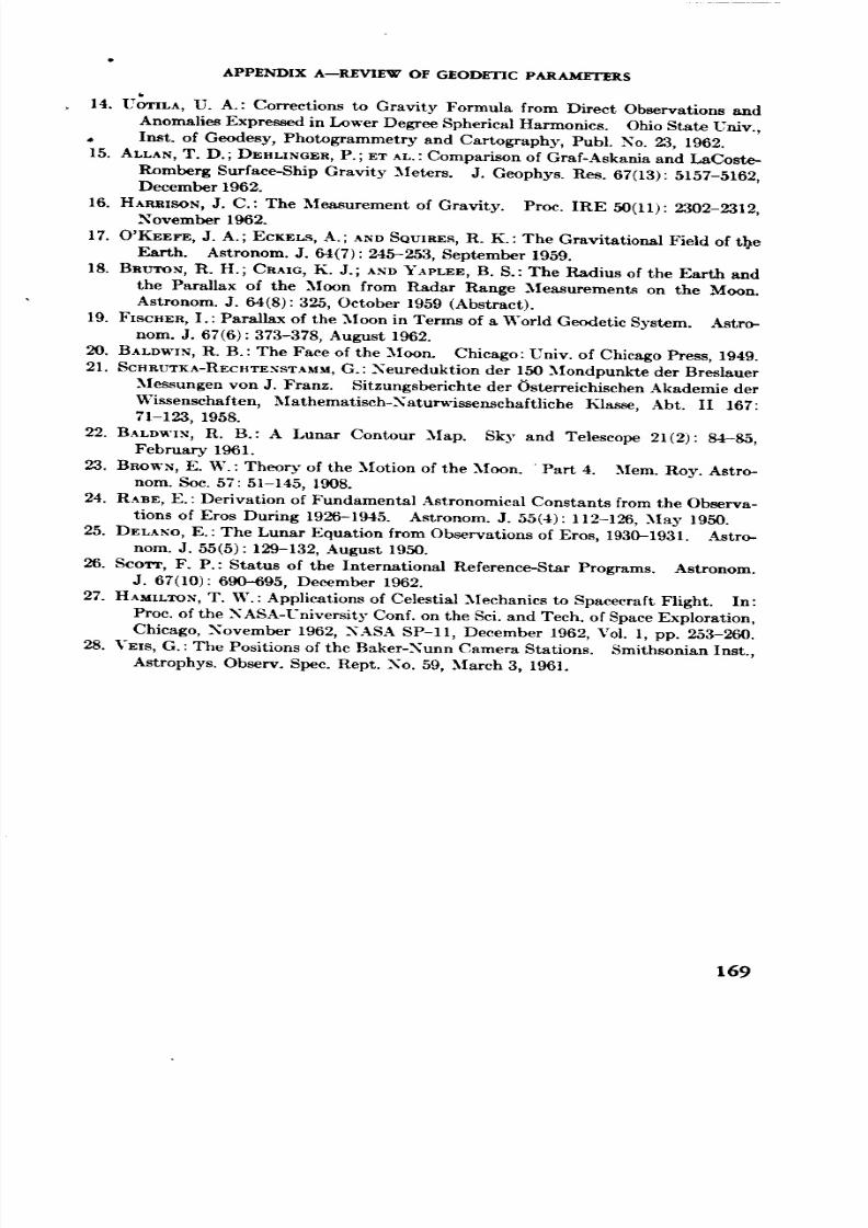
8/7/2019 Significant Achievements in Satellite Geodesy 1958-1964
http://slidepdf.com/reader/full/significant-achievements-in-satellite-geodesy-1958-1964 167/170
APPENDIX--REVIEWFGEODETICARAMETERS
14. U_rILA, U. A.: Corrections to Gravity Formula from Direct Observations and
Anomalies Expressed in Lower Degree Spherical Harmonics. Ohio State Univ.,
Inst. of Geodesy, Photogrammetry and Cartography, Publ. No. 23, 1962.
15. ALLAN, T. D. ; DERLING_H, P. ; ET AL. : Comparison of Graf-Askania and LaCoste-
Romberg Surface-Ship Gravity Meters. J. Geophys. Res. 67(13): 5157-5162,
December 1962.
16. HXRRISON, J. C.: The Measurement of Gravity. Proc. IRE 50(11): 2302-2312,
November 1962.
17. O'KEEFE, J. A. ; ECKEL% A. ; AND SQUIRES, R. K. : The Gravitational Field of the
Earth. Astronom. J. 64(7): 245-253, September 1959.
18. BRUTO,_, R. H.; CRAm, K. J.; A._D Y._PLEE, B. S.: The Radius of the Earth and
the Parallax of the Moon from Radar Range Measurements on the MooR.
Astronom. J. 64(8): 325, October 1959 (Abstract).
19. FISCHER, I. : Parallax of the Moon in Terms of a World Geodetic System. Astro-
nora. J. 67(6): 373-375, August 1962.
20. BALDWIN, R. B. : The Face of the .Moon. Chicago: Univ. of Chicago Press, 1949.
21. SCHaUTXA-RECHTE_ST._M, G.: Neureduktion der 150 Mondpunkte der Breslauer
Me_ungen von J. Franz. Sitzungsberiehte der Osterreichisehen Akademie der
Wissenschaften, Mathematiseh-Naturwissenschaftliche Klasse, Abt. II 167:
71-123, 1958.
22. BALVWIS, R. B.: A Lunar Contour Map. Sky and Telescope 21(2): 84-85,
February 1961.
23. BROWN, E. W. : Theory of the Motion of the Moon. Part 4. Mem. Roy. Astro-
nom. Soc. 57: 51-145, 1908.
24. RABE, E.: Derivation of Fundamental Astronomical Constants from the Observa-
tions of Eros During 1926-1945. Astronom. J. 55(4): 112-126, May 1950.
25. DZLAXO, E.: The Lunar Equation from Observations of Eros, 1930-1931. ._stro-
nom. J. 55(5): 129-132, August 1950.
26. SCOTT, F. P. : Status of the Interrmtional Reference-Star Programs. Astronom.
J. 67(10): 690-695, December 1962.
27. HAMILTON, T. W. : Applications of Celestial .Mechanics to Spacecraft Flight. In:
Proc. of the NASA-University Conf. on the Sci. and Tech. of Space Exploration,
Chicago, November 1962, NASA SP-11, December 1962, V01. 1, pp. 253-260.
28. VEIS, G. : The Positions of the Baker-Nunn Camera Stations. Smithsonian Inst.,
Astrophys. Observ. Spec. Rept. No. 59, March 3, 1961.
169

8/7/2019 Significant Achievements in Satellite Geodesy 1958-1964
http://slidepdf.com/reader/full/significant-achievements-in-satellite-geodesy-1958-1964 168/170
__ PAGE8U_K _ _D.
Appendix B
ReJerence List o] Recommended Constants

8/7/2019 Significant Achievements in Satellite Geodesy 1958-1964
http://slidepdf.com/reader/full/significant-achievements-in-satellite-geodesy-1958-1964 169/170
_.IECE:_G PAGE BI_IklR NOT FILIr_ED.
Reference List of Recommended Constants
Defining Constants
1. Number of ephemeris seconds in 1
tropical year (1900) ........ ......... s
2. Gaussian gravitational constant, defining
the a.u ............................ k
=31 556 925-9747
= 0.017 202 09895
Primary Constants
3. Measure of 1 a.u. in meters ............ A = 149 600)< 106
4. Velocity of light in meters per second.., c =299 792.5X10 s
5. Equatorial radius for Earth in meters.., a, =6 378 160
6. Dynamical form-factor for Earth ....... J2 = 0-001 082 7
7. Geocentric gravitational constant
(units: m s s-2) ...................... GE = 398 603 X 109
8. Ratio of the masses of the Moon and
Earth ............................. _ = 1/81.30
9. Sidereal mean motion of Moon in
radians per second (1900) ............ n(* = 2- 661 699 489 X 10 -e
10. General precession in longitude per
tropical century (1900) .............. p =5025:64
11. Obliquity of the ecliptic (1900) ......... e =23027'08:26
12. Constant of nutation (1900) ........... N =9:210
Auxiliary Constants and Factors
k/86400, for use when the unit of time is 1
second ................................. k'= 1.990 983 675X10 -7
Number of seconds of arc in 1 radian ......... 206 264-806
Factor for constant of aberration (note 15)... F1 = 1-000 142
Factor for mean distance of Moon (note 20).. F_ = 0.999 093 142
Factor ior paraiiactic m_qu,,,_'-...... 1:,., (_o_,_ ......._) F_=49853"._
173
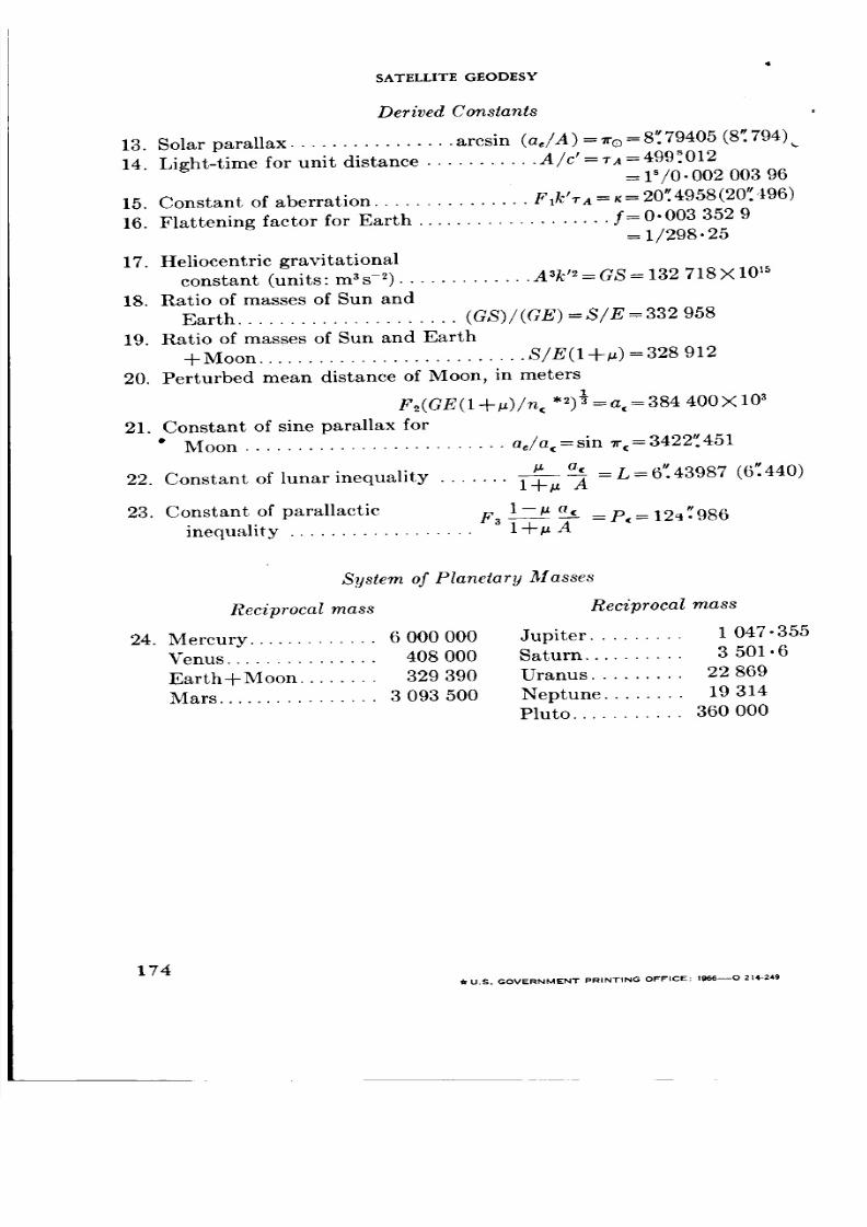
8/7/2019 Significant Achievements in Satellite Geodesy 1958-1964
http://slidepdf.com/reader/full/significant-achievements-in-satellite-geodesy-1958-1964 170/170
SATELLITE GEODESY
Derived Constants
13. Solar parallax ................ arcsin (ae/A) = ira = 8'.' 79405 (8". 794)
14. Light-time for unit distance ........... A/c' = TA=499_.012
= lS/0. 002 003 96
15. Constant of aberration ............... F1UTA = K= 20".4958(20'_496)
16. Flattening factor for Earth ................... f= 0.003 352 9
= 1/298-25
17. Heliocentric gravitational
constant (units: m 3s -2) ............. A3k '2= GS = 132 718 X 10 _5
18. Ratio of masses of Sun and
Earth ..................... (GS)/(GE) = S/E-- 332 958
19. Ratio of masses of Sun and Earth
+Moon .......................... S/E(1 +_) = 328 912
20. Perturbed mean distance of Moon, in meters1
F2(GE(1 +_)/n, *2)_ = a, = 384 400 X 103
21. Constant of sine parallax for
• Moon ......................... ae/a,=sin 7r(=3422'_451
a, = L = 6".43987 (6'.' 440)22. Constant of lunar inequality ....... l+tL A