Signals and Systems

Lecture 1

DR TANIA STATHAKIREADER (ASSOCIATE PROFESSOR) IN SIGNAL PROCESSINGIMPERIAL COLLEGE LONDON

Teacher’s coordinates

Teacher:

Dr. Tania Stathaki, Reader (Associate Professor) in Signal Processing,

Imperial College London

E-mail: t.stathaki@imperial.ac.uk

Office: 812

Logistics of the course

• Lectures - 15 hours over 8-9 weeks

• Problem Classes – 7-8 hours over 8-9 weeks

• Assessment – 100% by examination in June

• Handouts in the form of pdf slides are available at

http://www.commsp.ee.ic.ac.uk/~tania/

• Text Books:

- B.P. Lathi, “Linear Systems and Signals”, 2nd Ed., Oxford University

Press

- A.V. Oppenheim & A.S. Willsky “Signals and Systems”, Prentice

Hall

Aims and Objectives of Signals and Systems

• The concepts of signals and systems arise in a variety of fields such

as, communications, aeronautics, bio-engineering, energy, circuit

design and others.

• Although the physical attributes of the signals and systems involved in

the above disciplines are different, all signal and systems have basic

features in common.

• The aim of this course is to provide the fundamental and universal

tools for the analysis of signals.

• Furthermore, the course aims at teaching the analysis and design of

basic systems independently of the domain of application.

Aims and Objectives cont.

By the end of the course, you will have understood:

- Basic signal analysis

- Basic system analysis

- Time-domain system analysis including convolution

- Laplace and Fourier Transform

- System analysis in Laplace and Fourier domains

- Filter design

- Sampling theory

- Basics on z-transform

Today’s Lecture

In this lecture we will talk about:

• Examples of signals

• Some useful signal operations

• Classification of signals

• Some specific widely used signals:

▪ Unit step function

▪ Unit impulse function

▪ The exponential function

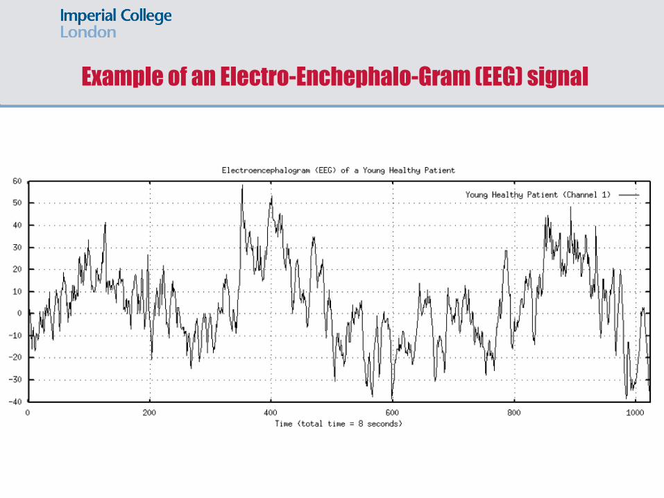
Example of an Electro-Enchephalo-Gram (EEG) signal

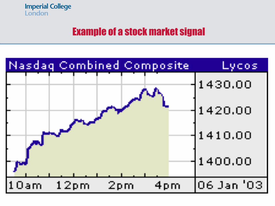
Example of a stock market signal

Magnetic Resonance Image (MRI).

This is a signal in 2 dimensions.

Useful signal operations: time shifting

• Consider a signal 𝑥(𝑡) in continuous –

time shown in the figure right.

• The signal 𝑥 𝑡 may be delayed

by 𝑇 units of time; in that case

the signal 𝜙 𝑡 = 𝑥(𝑡 − 𝑇) is obtained.

• The signal 𝑥 𝑡 may be advanced

by 𝑇 units of time; in that case

the signal 𝜙 𝑡 = 𝑥(𝑡 + 𝑇) is obtained.

Useful signal operations cont.: time scaling

• Consider a signal 𝑥(𝑡) in continuous –

time shown in the figure right.

• The signal 𝑥 𝑡 may be compressed

by a factor of 2; in that case

the signal 𝜙 𝑡 = 𝑥(2𝑡) is obtained.

• The signal 𝑥 𝑡 may be stretched

by a factor of 2; in that case

the signal 𝜙 𝑡 = 𝑥𝑡

2is obtained.

Classification of signals

• Signals may be classified into:

▪ Energy and power signals

▪ Discrete – time and continuous – time signals

▪ Analogue and digital signals

▪ Deterministic and probabilistic signals

▪ Periodic and aperiodic signals

▪ Even and odd signals

Energy of a signal

• How do we measure the “size” of a signal 𝑥(𝑡)?

▪ By the signal energy 𝐸𝑥

𝐸𝑥 = න

−∞

∞

𝑥2 𝑡 𝑑𝑡

▪ For a complex-valued signal the above relationship becomes:

𝐸𝑥 = න

−∞

∞

𝑥2 𝑡 𝑑𝑡

▪ The energy of a signal must be finite. This implies that:

lim𝑡→±∞

𝑥(𝑡) = 0

Power of a signal

▪ If lim𝑡→±∞

𝑥(𝑡) ≠ 0 we must use the signal power instead

𝑃𝑥 = lim𝑇→∞

1

𝑇න

−𝑇2

𝑇2

𝑥2 𝑡 𝑑𝑡

▪ For a complex – valued signal the above relationship becomes:

𝑃𝑥 = lim𝑇→∞

1

𝑇න

−𝑇2

𝑇2

𝑥2 𝑡 𝑑𝑡

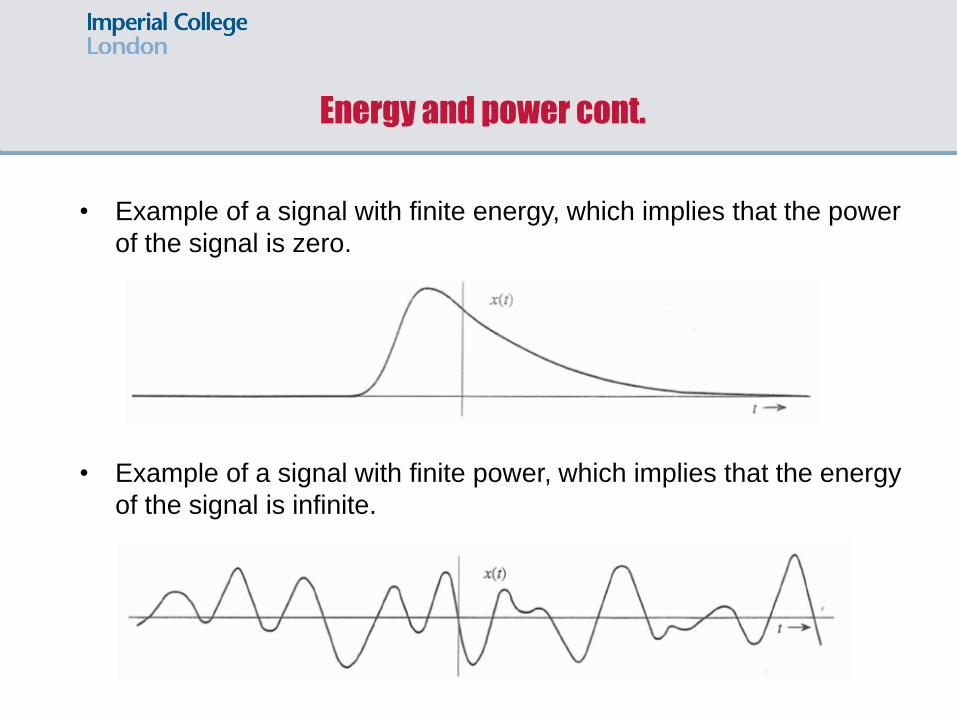
Energy and power cont.

• Example of a signal with finite energy, which implies that the power

of the signal is zero.

• Example of a signal with finite power, which implies that the energy

of the signal is infinite.

Continuous – and Discrete – Time SignalsThis classification refers to time 𝒕

• Example of a continuous – time

signal. This is defined for any

value of time.

• Example of a discrete – time

signal.

▪ This is defined for certain

instants of time only.

▪ It arises from a continuous – time

signal if only its values at these

certain time instants are kept.

▪ This process is called sampling.

Analog and Digital SignalsThis classification refers to the value of the signal 𝒙(𝒕)

• An analog signal can take infinite

number of values.

• A digital signal can take only a

finite number of values.

▪ It arises from an analog

signal if all values are replaced

with a finite number of values.

▪ The total error arising from this

process must be as small as

possible.

▪ This process is called

quantization.

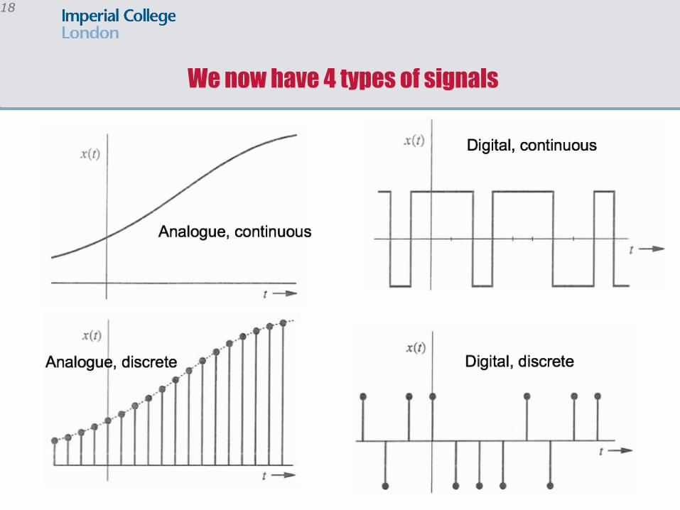
18

We now have 4 types of signals

Periodic and Aperiodic Signals

• A signal is said to be periodic if for some constant 𝑇0 the following

condition holds:

𝑥 𝑡 + 𝑇0 = 𝑥 𝑡 , ∀𝑡

• The smallest 𝑇0 that satisfies the above relationship is called the

fundamental period of the signal.

Even and Odd Signals

• An even signal remains the same if you rotate it along the vertical axis. In

mathematical terms this property is defined as 𝑥 −𝑡 = 𝑥(𝑡).

• An odd signal gets reflected along the horizontal axis if you rotate it along

the vertical axis. In mathematical terms this property is defined as

𝑥 −𝑡 = −𝑥(𝑡).

Even and Odd Signals

Easy problems

• Verify that the signal 𝑥 𝑡 + 𝑥(−𝑡) is always even.

• Verify that the signal 𝑥 𝑡 − 𝑥(−𝑡) is always odd.

Based on the above, any signal can be written as a the sum of an even

and an odd signal as follows:

𝑥 𝑡 =1

2𝑥 𝑡 + 𝑥(−𝑡) +

1

2𝑥 𝑡 − 𝑥(−𝑡)

Deterministic and Stochastic Signals

• The values of a deterministic signal can be obtained from a closed –

form mathematical expression. For example, 𝑥 𝑡 = sin 𝑡 .

• The values of a stochastic signal can only be given as the outputs of a

probabilistic model.

Experiment. Drop a coin 1000 times and create the following 1000 – sample

digital signal: Every time you get head the value of your signal will be +1, every

time you get tails the value of your signal will be −1.

▪ Can you tell what is the value of the signal at time instant 𝑛?

▪ Can you tell the probability of the value being +1 or −1?

▪ What is approximately the mean (average value) of the signal you created?

Unit step function

• The unit step function is defined as follows:

𝑢 𝑡 = ቊ1 𝑡 ≥ 00 𝑡 < 0

• The unit step function is often used to describe a signal that starts at

𝑡 = 0.

• For example, consider the everlasting exponential signal 𝑥 𝑡 = 𝑒−𝑡.

• The causal form of the above signal is 𝑒−𝑡𝑢(𝑡).

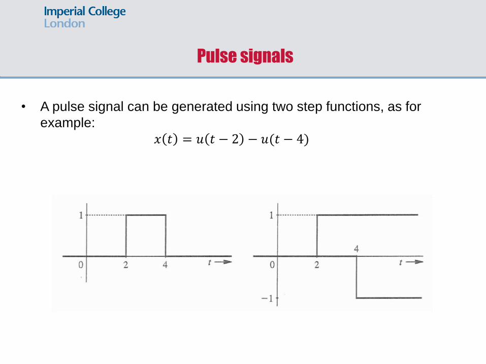
Pulse signals

• A pulse signal can be generated using two step functions, as for

example:

𝑥 𝑡 = 𝑢 𝑡 − 2 − 𝑢(𝑡 − 4)

Unit impulse (Dirac) function

• The Dirac function is defined as follows:

𝛿 𝑡 = 0, 𝑡 ≠ 0

න

−∞

∞

𝛿 𝑡 𝑑𝑡 = 1

• The Dirac function is the limit of a family of functions 𝛿𝜖(𝑡) when 𝜖 → 0.The simplest of these functions is the rectangular pulse shown in the

figure below right. The width and height depend on 𝜖 but the entire area

under the function is equal to 1.

Sampling property of the unit impulse function

• Since the unit impulse function is non – zero only at 𝑡 = 0, for any

function 𝜙(𝑡) we have

𝜙 𝑡 𝛿 𝑡 = 𝜙 0 𝛿 𝑡

• From the above we get:

∞−∞

𝜙 𝑡 𝛿 𝑡 𝑑𝑡 = ∞−∞

𝜙 0 𝛿 𝑡 𝑑𝑡 = 𝜙 0 ∞−∞

𝛿 𝑡 𝑑𝑡 = 𝜙 0

• Furthermore, we have:

∞−∞

𝜙 𝑡 𝛿 𝑡 − 𝑇 𝑑𝑡 = ∞−∞

𝜙 𝜏 + 𝑇 𝛿 𝜏 𝑑𝜏 = 𝜙 𝑇

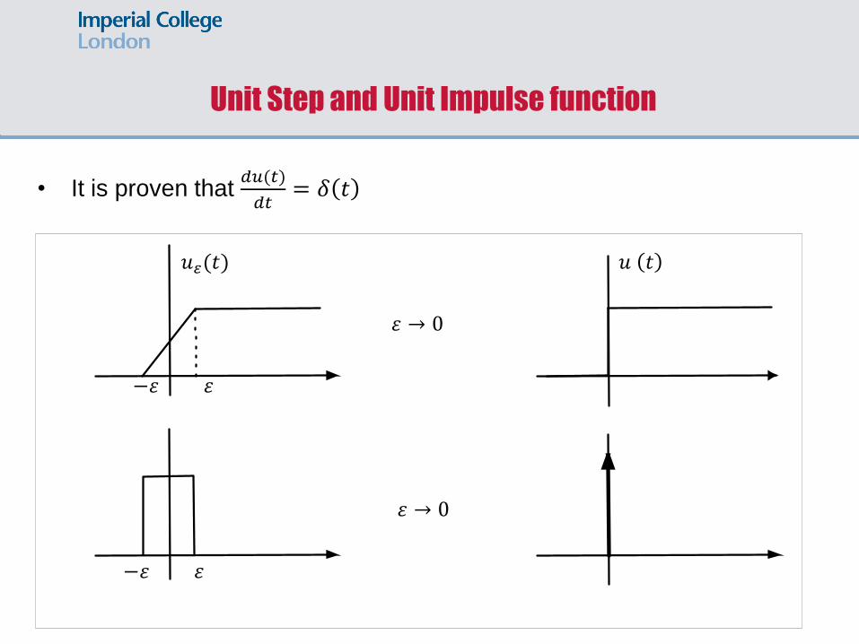
• It is proven that 𝑑𝑢(𝑡)

𝑑𝑡= 𝛿 𝑡

𝑢𝜀(𝑡) 𝑢 𝑡

휀 → 0

−휀 휀

휀 → 0

−휀 휀

Unit Step and Unit Impulse function

The Exponential Function 𝒆𝒔𝒕

• The exponential function is very important in science and engineering.

• The parameter 𝑠 is a complex variable given by 𝑠 = 𝜎 + 𝑗𝜔.

• Therefore, 𝑒𝑠𝑡 = 𝑒 𝜎+𝑗𝜔 𝑡 = 𝑒𝜎𝑡 𝑒𝑗𝜔𝑡 = 𝑒𝜎𝑡(cos𝜔𝑡 + 𝑗sin𝜔𝑡)

• If 𝑠∗ is the complex conjugate of 𝑠 then 𝑠 = 𝜎 − 𝑗𝜔

𝑒𝑠∗𝑡 = 𝑒 𝜎−𝑗𝜔 𝑡 = 𝑒𝜎𝑡 𝑒−𝑗𝜔𝑡 = 𝑒𝜎𝑡(cos𝜔𝑡 − 𝑗sin𝜔𝑡)

𝑒𝜎𝑡cos𝜔𝑡 =1

2𝑒𝑠𝑡 + 𝑒𝑠

∗𝑡

𝑒𝜎𝑡sin𝜔𝑡 =1

2𝑗𝑒𝑠𝑡 − 𝑒𝑠

∗𝑡

• The exponential function can be used to model a large class of signals.

▪ A constant 𝑘 = 𝑘𝑒0𝑡, 𝑠 = 0

▪ A monotonic real exponential 𝑒𝜎𝑡, 𝑠 = 𝜎, 𝜔 = 0

▪ A complex sinusoid cos𝜔𝑡 ± 𝑗sin𝜔𝑡, 𝜎 = 0, 𝑠 = ±𝑗𝜔

▪ An exponentially varying real sinusoid 𝑒𝜎𝑡cos𝜔𝑡 = Re{𝑒𝑠𝑡}, 𝑠 = 𝜎 ± 𝑗𝜔

Discrete-Time Exponential 𝜸𝒏

• A continuous − time exponential 𝑒𝑠𝑡 can be expressed in alternate

form as 𝑒𝑠𝑡 = 𝛾𝑡 with 𝛾 = 𝑒𝑠.

• Similarly for discrete time exponentials we have 𝑒𝜆𝑛 = 𝛾𝑛.

• When Re 𝜆 < 0 then 𝑒𝜆 = 𝛾 < 1 and the exponential decays.

• When Re 𝜆 > 0 then 𝑒𝜆 = 𝛾 > 1 and the exponential grows.

• When Re 𝜆 = 0 then 𝑒𝜆 = 𝛾 = 1. The exponential is of constant-

amplitude and oscillates.

• If we depict 𝜆 and 𝛾 in the two – dimensional plane, we can see the

mapping between the two variables (look at next slide).

Discrete-Time Exponential 𝜸𝒏 cont.

Mapping from 𝜆 to 𝛾

I hope you enjoyed this lecture.

Thank you for attending and see you

again in the next class!