signal is enough. a photograph taken by the “single-pixel camera” builtby richard baraniuk and...

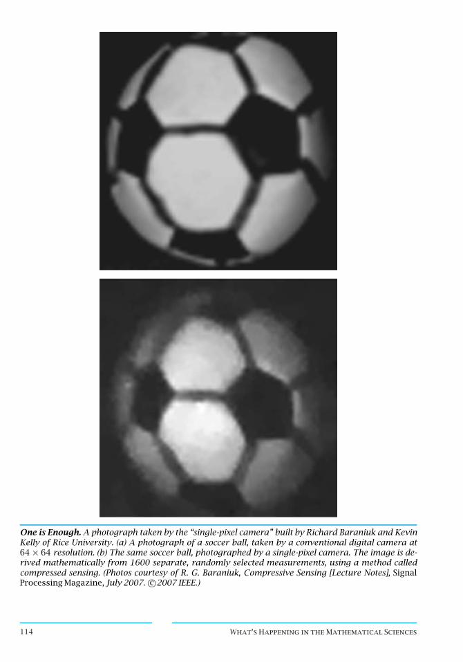
One is Enough. A photograph taken by the “single-pixel camera” built by Richard Baraniuk and KevinKelly of Rice University. (a) A photograph of a soccer ball, taken by a conventional digital camera at64 × 64 resolution. (b) The same soccer ball, photographed by a single-pixel camera. The image is de-rived mathematically from 1600 separate, randomly selected measurements, using a method calledcompressed sensing. (Photos courtesy of R. G. Baraniuk, Compressive Sensing [Lecture Notes], SignalProcessing Magazine, July 2007. c©2007 IEEE.)

114 What’s Happening in the Mathematical Sciences

Compressed Sensing MakesEvery Pixel Count

Trash and computer files have one thing in common:compact isbeautiful. But if you’ve ever shoppedfora digi-tal camera, you might have noticed that camera manufac-

turers haven’t gotten the message. A few years ago, electronicstores were full of 1- or 2-megapixel cameras. Then along camecameras with 3-megapixel chips, 10 megapixels, and even 60megapixels.

Unfortunately, these multi-megapixel cameras create enor-mous computer files. So the first thing most people do, if theyplan to send a photo by e-mail or post it on the Web, is to com-pact it to a more manageable size. Usually it is impossible todiscern the difference between the compressed photo and theoriginal with the naked eye (see Figure 1, next page). Thus, astrange dynamic has evolved, in which camera engineers cram

Emmanuel Candes. (Photo cour-tesy of Emmanuel Candes.)

more and more data onto a chip, while software engineers de-sign cleverer and cleverer ways to get rid of it.

In 2004, mathematicians discovered a way to bring this“arms race” to a halt. Why make 10 million measurements, theyasked, when you might need only 10 thousand to adequatelydescribe your image? Wouldn’t it be better if you could justacquire the 10 thousand most relevant pieces of informationat the outset? Thanks to Emmanuel Candes of Caltech, Ter-ence Tao of the University of California at Los Angeles, JustinRomberg of Georgia Tech, and David Donoho of StanfordUniversity, a powerful mathematical technique can reduce thedata a thousandfold before it is acquired. Their technique,called compressed sensing, has become a new buzzword inengineering, but its mathematical roots are decades old.

As a proof of concept, Richard Baraniuk and Kevin Kelly ofRice University even developed a single-pixel camera. However,don’t expect it to show up next to the 10-megapixel camerasat your local Wal-Mart because megapixel camera chips have abuilt-in economic advantage. “The fact that we can so cheaplybuild themisdue toa very fortunate coincidence, that the wave-lengths of light that our eyes respond to are the same onesthatsiliconresponds to,” saysBaraniuk. “Thishasallowedcam-era makers to jump on the Moore’s Law bandwagon”—in otherwords, to double the number of pixels every couple of years.

Thus, the true market for compressed sensing lies in non-visible wavelengths. Sensors in these wavelengths are not socheap to build, and they have many applications. For example,cell phones detect encoded signals from a broad spectrum ofradio frequencies. Detectors of terahertz radiation1 could beused to spot contraband or concealed weapons under clothing.

1This is a part of the electromagnetic spectrum that could either bedescribed as ultra-ultra high frequency radio or infra-infrared light,depending on your point of view.

What’s Happening in the Mathematical Sciences 115

Figure 1. Normal scenes from everyday life are compressible with respect to a basis of wavelets. (left)A test image. (top) One standard compression procedure is to represent the image as a sum of wavelets.Here, the coefficients of the wavelets are plotted, with large coefficients identifying wavelets that make asignificant contribution to the image (such as identifying an edge or a texture). (right) When the waveletswith small coefficients are discarded and the image is reconstructed from only the remaining wavelets,it is nearly indistinguishable from the original. (Photos and figure courtesy of Emmanuel Candes.)


Even conventional infrared light is expensive to image. “Whenyou move outside the range where silicon is sensitive, your$100 camera becomes a $100,000 camera,” says Baraniuk.In some applications, such as spacecraft, there may not beenough room for a lot of sensors. For applications like these, itmakes sense to think seriously about how to make every pixelcount.

The Old ConventionalWisdomThe story of compressed sensing begins with Claude Shannon,the pioneer of information theory. In 1949, Shannon provedthat a time-varying signal with no frequencies higher than Nhertz can be perfectly reconstructed by sampling the signal atregular intervals of 1/2N seconds. But it is the converse theo-

Terence Tao. (Photo courtesy ofReed Hutchinson/UCLA.)

rem that became gospel to generations of signal processors: asignal with frequencies higher than N hertz cannot be recon-structed uniquely; there is always a possibility of aliasing (twodifferent signals that have the same samples).

In the digital imaging world, a “signal” is an image, and a“sample” of the image is typically a pixel, in other words a mea-surement of light intensity (perhaps coupled with color infor-mation) at a particular point. Shannon’s theorem (also calledthe Shannon-Nyquist sampling theorem) then says that the res-olution of an image is proportional to the number of measure-ments. If you want to double the resolution, you’d better dou-ble the number of pixels. This is exactly the world as seen bydigital-camera salesmen.

Candes, Tao, Romberg, and Donoho have turned that worldupside down. In the compressed-sensing view of the world, theachievable resolution is controlled primarily by the informa-tion content of the image. An image with low information con-tent can be reconstructed perfectly from a small number ofmeasurements. Once you have made the requisite number ofmeasurements, it doesn’t help you to add more. If such imageswere rare or unusual, this news might not be very exciting. Butin fact, virtually all real-world images have low information con-tent (as shown in Figure 1).

This point may seem extremely counterintuitive because themathematical meaning of “information” is nearly the oppositeof the common-sense meaning. An example of an image withhigh information content is a picture of random static on a TVscreen. Most laymen would probably consider such a signal tocontain no information at all! But to a mathematician, it hashigh information content precisely because it has no pattern;in order to describe the image or distinguish between two suchimages, you literally have to specify every pixel. By contrast,any real-world scene has low information content because it ispossible to convey the content of the image with a small num-ber of descriptors. A few lines are sufficient to convey the ideaof a face, and a skilled artist can create a recognizable likenessof any face with a relatively small number of brush strokes.2

2The modern-day version of the “skilled artist” is an image compres-sion algorithm, such as the JPEG-2000 standard, which reconstructsa copy of the original image from a small number of componentscalled wavelets. (See “Parlez-vous Wavelets?” in What’s Happening inthe Mathematical Sciences, Volume 2.)


The idea of compressed sensing is to use the low infor-mation content of most real-life images to circumvent theShannon-Nyquist sampling theorem. If you have no infor-mation at all about the signal or image you are trying toreconstruct, then Shannon’s theorem correctly limits the res-olution that you can achieve. But if you know that the image issparse or compressible, then Shannon’s limits do not apply.

Long before “compressed sensing” became a buzzword,there had been hints of this fact. In the late 1970s, seismicengineers started to discover that “the so-called fundamen-tal limits weren’t fundamental,” says Donoho. Seismologistsgather information about underground rock formations bybouncing seismic waves off the discontinuities between strata.(Any abrupt change in the rock’s state or composition, such

Justin Romberg. (Photo courtesyof Justin Romberg.)

as a layer of oil-bearing rock, will reflect a vibrational waveback to the surface.) In theory the reflected waves did notcontain enough information to reconstruct the rock layersuniquely. Nevertheless, seismologists were able to acquirebetter images than they had a right to expect. The ability to “seeunderground” made oil prospecting into less of a hit-or-missproposition. The seismologists explained their good fortunewith the “sparse spike train hypothesis,” Donoho says. The hy-pothesis is that underground rock structures are fairly simple.At most depths, the rock is homogeneous, and so an incomingseismic wave sees nothing at all. Intermittently, the seismicwaves encounter a discontinuity in the rock, and they return asharp spike to the sender. Thus, the signal is a sparse sequenceof spikes with long gaps between them.

In this circumstance, it is possible to beat the constraints ofShannon’s theorem. It may be easier to think of the dual sit-uation: a sparse wave train that is the superposition of justa few sinusoidal waves, whose frequency does not exceed Nhertz. If there are K frequency spikes in a signal with maximalfrequency N, Shannon’s theorem would tell you to collect Nequally spaced samples. But the sparse wave train hypothesislets you get by with only 3K samples, or even sometimes just2K. The trick is to sample at random intervals, not at regular in-tervals (see Figures 2 and 3). If K <<N (which is the meaning of a“sparse” signal), then random sampling is much more efficient.

In other fields, such as magnetic resonance imaging, re-searchers also found that they could “undersample” the dataand still get good results. At scientific meetings, Donoho says,they always encountered skepticism because they were try-ing to do something that was supposed to be impossible. Inretrospect, he says that they needed a sort of mathematical“certificate,” a stamp of approval that would guarantee whenrandom sampling works.

The New CertificateEmmanuelCandes, a formerstudentofDonoho, faced the sameskepticism in 2004, while working with a team of radiologistson magnetic resonance imaging. In trial runs with a “phantomimage” (in other words, not a real patient), he was able to recon-struct the image perfectly fromundersampleddata. “There wasno discrepancy at all between the original and the reconstruc-tion,” Candes says. “I actually got into a bit of trouble, becausethey thought I was fudging.”


Figure 2. Reconstructing a sparse wave train. (a) The frequency spectrum of a 3-sparse signal. (b) Thesignal itself, with two sampling strategies: regular sampling (red dots) and random sampling (blue dots).(c) When the spectrum is reconstructed from the regular samples, severe “aliasing” results because thenumber of samples is 8 times less than the Shannon-Nyquist limit. It is impossible to tell which frequen-cies are genuine and which are impostors. (d) With random samples, the two highest spikes can easilybe picked out from the background. (Figure courtesy of M. Lustig, D. Donoho, J.Santos and J. Pauly,Compressed Sensing MRI, Signal Processing Magazine, March 2008. c©2008 IEEE.)

Figure 3. In the situation of Figure 2, the third frequency spike can be recovered by an iterative thresh-olding procedure. If the signal was known to be 3-sparse to begin with, then the signal can be recon-structed perfectly, in spite of the 8-fold undersampling. In short, sparsity plus random sampling enablesperfect (or near-perfect) reconstruction. (Figure courtesy of M. Lustig, D. Donoho, J.Santos and J. Pauly,Compressed Sensing MRI, Signal Processing Magazine, March 2008. c©2008 IEEE.)


At this point, Candes did a fortuitous thing: he talked withCandesandTaofoundashortcut thatnotonlyruns fasteronacomputer,butalsoexplainswhyrandomsamplingworkssomuchbetter thanregularsampling.

Terry Tao, a 2006 Fields medalist. The two mathematicianshappened to have children at the same pre-school. While theywere dropping them off one day, Candes told Tao about thetoo-good-to-be-true reconstructions. “I had begun looking foran explanation and made some headway, but I was stuck at aparticular point,” Candes says.

“Terry reacted like a mathematician,” Candes continues. “Hesaid, ‘I’m going to find a counterexample, showing that whatyou have in mind cannot be true.”’ But a strange thing hap-pened. None of the counterexamples seemed to work, and Taostarted listening more closely to Candes’ reasoning. “After awhile, he looked at me and said, ‘Maybe you’re right,”’ Candessays. With the speed for which Tao is legendary, within a fewdays he had helped Candes overcome his obstacle and the twoof them began to sketch out the first truly general theory ofcompressed sensing.

In the Candes-Romberg-Tao framework, a signal or an im-age is represented as a vector x, a string of N real numbers.This vector is assumed to be K-sparse, which means that insome prescribed basis it is known to have at most K nonzerocoefficients. (K is assumed to be much less than N.) For exam-ple, if the basis elements are standard coordinate vectors inRN , then x literally consists of mostly zeroes. This is exactly thesituation of the sparse spike train hypothesis.

However, compressed sensing does not require a particu-lar basis. Photographs, for example, are not at all sparse withrespect to the standard basis; they have many nonzero coef-ficients (i.e., non-black pixels). JPEG compression has proventhat photographs are almost always approximatelysparse withrespect to a different basis—the basis of wavelets. If Ψ repre-sents theN ×N matrix of basis vectors, then aK-sparse signalwith respect to that basis is one that can be written in the formΨx, where x has at mostK nonzero coefficients.

A sample y of the signal x, in the Candes-Romberg-Taoframework, is a linear function of x: that is, y = Φx. The num-ber of measurements in the sample is assumed to be smallerthan the signal, so Φ is an M × N matrix with M < < N. By ele-mentary linear algebra, there are infinitely many other vectorsx∗ such that Φx∗ = y. However, provided thatM ≥ 2K, it willnormally be the case that none of the other solutions to theequation Φx∗ = y are sparse. Thus, if x is known in advanceto be sparse, it can in theory be reconstructed exactly from Mmeasurements.

Knowing that a unique solution exists is not the same thingas being able to find it. The problem is that there is no way toknow in advance which K coordinates of x are nonzero. Thenaive approach is to try all the possibilities until you hit on theright one, but this turns out to be a hopelessly slow algorithm.However, Candes and Tao found a shortcut that not only runsfaster on a computer, but also explains why random samplingworks so much better than regular sampling.

If your image consists of a few sparse dots or a few sharplines, the worst way to sample it is by capturing individual pix-els (the way a regular camera works!). The best way to sample


the image is to compare it with widely spread-out noise func-tions. One could draw an analogy with the game of “20 ques-tions.” If you have to find a number between 1 and N, the worstway to proceed is to guess individual numbers (the analog ofmeasuring individual pixels). On average, it will take you N/2

Figure 4. A random measurement of a sparse signal, S, gener-ates a subspace of possible signals (green) that could have pro-duced that measurement.Within that green subspace, the vectorof smallest l1-norm (S) is usually equal to S. (Figure courtesy ofR. G. Baraniuk, Compressive Sensing [Lecture Notes], Signal Pro-cessing Magazine, July 2007. c©2007 IEEE.)

guesses. By contrast, if you ask questions like, “Is the numberless than N/2?” and then “Is the number less than N/4?” andso on, you can find the concealed number with at most log2 Nquestions. If N is a large number, this is an enormous speed-up.

Notice that the “20 questions” strategy is adaptive: youare allowed to adapt your questions in light of the previousanswers. To be practically relevant, Candes and Tao neededto make the measurement process nonadaptive, yet with thesame guaranteed performance as the adaptive strategy justdescribed. In other words, they needed to find out ahead oftime what would be the most informative questions about thesignal x. That this can be done effectively is one of the greatsurprisesof the new theory. The idea of their approach is calledl1-minimization.

The l0-norm of a vector is simply the number of nonzero en-tries in the vector, which can be somewhat informally writtenas follows:

‖(x1, x2, ..., xN)‖0 =∑

|xi|0.


(This formula uses the convention that 00 = 0.) The l1-norm isobtained by replacing the 0’s in this equation by 1’s:

‖(x1, x2, ..., xN)‖1 =∑

|xi|1.

In this language, the signal x is the unique solution toΦx∗ =y with the smallest l0-norm. But in many cases, Candes and Taoproved, it is also the unique solution with the smallest l1-norm.This was a critical insight because l1-minimization is a linearprogramming problem, which can be solved by known, efficient

Arandomplane thatpasses throughavertexisvirtuallycertain tomiss the interiorof thecrosspolytope.Thanksto this “miracleofhigh-dimensionalgeometry,” asCandescalls it, the l1-minimizerwill almostalwaysbethecorrect signal, x.

computer algorithms. (See “Smooth(ed) Moves,” What’s Hap-pening in the Mathematical Sciences, Volume 6.)

Figure 4 illustrates why the l1-minimizer is often the sameas the l0-minimizer. In 3-dimensional space, the set of unit vec-tors in the l1-norm is an octahedron. Think of the sparse vec-tor x as lying on a coordinate axis (because it has lots of zerocoordinates). Therefore it is at one of the vertices of the oc-tahedron. The set of vectors x∗ such that Φx∗ = y is a planepassing through the point x. Most planes that pass through xintersect the octahedron only at the point x; in other words, xis the unique point on the plane with the minimum l1-norm. Soif you simply pick the measurementΦ “at random,” you have avery good chance of reconstructing x uniquely.

Unfortunately, pickingΦ at random won’t always work. Youmight get unlucky and choose a plane through x that passesthrough the interior of the octahedron. If so, the l1-minimizerwill not be the same as the l0-minimizer. The algorithm willproduce an erroneous signal, x∗. But the three-dimensional pic-ture in Figure 4 (page 121) is somewhat misleading because theimage vectors typically lie in a space with thousands or mil-lions of dimensions. The analog of the octahedron in million-dimensional space is called the cross polytope; and in million-dimensional space the cross polytope is very, very, very pointy.A random plane that passes through a vertex is virtually cer-tain to miss the interior of the cross polytope. Thanks to this“miracle of high-dimensional geometry,” as Candes calls it, thel1-minimizer will almost always be the correct signal, x.

In summary, this is what the theory of compressed sensingsays:

• For many M × N matrices Φ, the unique K-sparse so-lution, x, to the equation Φx∗ = y, can be recoveredexactly.

• N must be much larger than K. However, M (the num-ber of measurements) need only be a little larger thanK. Specifically, M must be roughly K log(N/K). Noticethat the dependence on N is logarithmic, so the “20questions” speed-up has been achieved.

• The K-sparse solution is found by l1-minimization,whichcanbe proved tobe equivalent to l0-minimizationunder certain assumptions on the measurement ma-trix,Φ.

• Random matrices Φ almost always satisfy those as-sumptions.

The whole story remains essentially unchanged if the sig-nal is sparse with respect to a basis Ψ that is not the standardbasis of coordinate vectors (e.g., the wavelet basis). The only


modification required is that the constraint, Φx∗ = y, is re-placed by the constraintΦΨx∗ = y. In this context, the random-ness of the measurement matrix Φ serves a double purpose.First, it provides the easiest set of circumstances under whichl1-minimization is provably equivalent to l0-minimization. Sec-ondly, and independently, it ensures that the set of measure-ment vectors (the rows ofΦ) are as dissimilar to the image basis(the columns of Ψ ) as possible. If the image basis consists ofspikes, the measurement basis should consist of spread-outrandom noise. If the image basis consists of wavelets, then themeasurement basis should consist of a complementary type ofsignal called “noiselets.”

“Our paper showed something really unexpected,” says Can-des. “It showed that using randomness as a sensing mechanismis extremely powerful. That’s claim number one. Claim numbertwo is that it is amenable to rigorous analysis.

“What mathematicians liked [about the paper] was the wayit merged analysis and probability theory. A lot of people inmy field, analysis, did not think about probability theory as be-ing useful or worthy of attention. At the very intellectual level,it changed the mindset of those people and caused them toengage this field.”

Richard Baraniuk. (Photo cour-tesy of Richard Baraniuk.)Recent Developments

Tao and Candes’ preprint appeared in 2004, as did a paper byDonoho announcing similar results. By the time that Tao andCandes’ paper actually appeared in print, in 2006, it had beencited more than 100 times. Since then, there have been manyadvances, both from the theoretical and the practical side.

One question left unanswered by the original paper washow well compressed sensing would hold up if the measure-ments contained some random error (an inevitable problemof real-world devices), or if the images themselves were notexactly sparse. In photography, for instance, the assumptionof a sparse signal is not literally true. It is more realistic toassume the signal is compressible, which means that the vastmajority of the information in the signal is contained in afew coefficients. The remaining coefficients are not literallyzero, but they are small. Under these circumstances, even thel0-minimizer does not match the signal exactly, so there is nohope for the l1-minimizer to be exactly correct.

In 2005, Candes, Romberg, and Tao showed that evenwith noisy measurements and compressible (but not sparse)signals, compressed sensing works well. The error in the re-constructed signal will not be much larger than the error in themeasurements, and the error due to using the l1-minimizer willnot be much greater than the penalty already incurred by thel0-minimizer. That is, the l1-minimizer accurately recovers themost important pieces of information, the largest componentsof the signal. Figure 5 (see next page) shows an example ofthe performance of compressed sensing on a simulated imagewith added noise.

Mathematicians have also been working on new algorithmsthat run even faster than the standard linear programmingtechniques that solve the l1-minimization problem. Insteadof finding the largest K coefficients of x all at once, they findthem iteratively: first the largest nonzero coefficient, then the


Figure 5. Compressed sensing with noisy data. (a) An image with added noise. (b) The image, under-sampled and reconstructed using the Shannon-Nyquist approach. As in Figure 2, artifacts appear in thereconstructed image. (d) The same image, undersampled randomly and reconstructed with a “too opti-mistic” noise model. Although there are no artifacts, some of the noise has been misinterpreted as realvariation. (c) The same image, reconstructed from a random sample with a more tolerant noise model.The noise is suppressed and there are no artifacts. (Figure courtesy of Michael Lustig.)


second-largest one, and so on. The first such algorithm, calledOrthogonal Matching Pursuit (OMP), did not offer the sameguarantees of accuracy that l1-minimization did. However,there is now a variety of colorfully named variations, such asRegularized OMP (ROMP) and Stagewise OMP (StOMP), whichsuccessfully combine the accuracy of l1-minimization with thespeed of OMP. These algorithms have the advantage of beingsomewhat more intuitive than the “high-dimensional miracle”of l1-minimization; Figure 3 shows an example.

Meanwhile, researchers in several different fields are explor-ing practical applications of compressed sensing. Baraniukand Kelly’s single-pixel camera, built in 2006, uses an arrayof bacteria-sized mirrors to acquire a random sample of theincoming light. (See Figure 6.) Each mirror can be tilted in oneof two ways, either to reflect the light toward the single sensoror away from it. Thus the light that the sensor receives is aweighted average of many different pixels, all combined intoone pixel. By taking K log(N/K) snapshots, with a differentrandom selection of pixels each time, the single-pixel camerawas able to acquire a recognizable picture with a resolutioncomparable to N pixels. (See figure “One Is Enough,” page 114.)

Baraniuk and Kelly’s team is now working on “hyperspec-tral cameras,” which would reconstruct a complete spectrumat each point of the image. “A conventional digital image hasred, blue and green pixels,” Baraniuk says. “It’s great for mak-ing a picture that fools the human eye, but it doesn’t capturethe essence of the wavelengths given off by different materi-als. What you’d really like would be a spectrum of thousandsof colors instead of just three. This would allow you to tell thedifference between green paint on a car and a green leaf ona bush.” But with thousands of colors at each of millions ofpixels, data compression becomes a serious issue.

Figure 6. A schematic diagram of the “one-pixel camera.” The “DMD” is the grid of micro-mirrors thatreflect some parts of the incoming light beam toward the sensor, which is a single photodiode. Otherparts of the image (the black squares) are diverted away. Each measurement made by the photodiode isa random combination of many pixels. In “One is Enough” (p.114), 1600 random measurements sufficeto create an image comparable to a 4096-pixel camera. (Figure courtesy of Richard Baraniuk.)


Baraniuk and his former student Michael Wakin, now at theUniversity of Michigan, have also worked on a problem of ob-Withsomanyquestions

andsomanychoices, itis impossibleatpresenttosaywhat themostsuccessfulapplicationofcompressedsensingwillbe.However,onething isclear:Engineersarefinally thinkingoutside theboxofShannon’s theorem.

ject detection. For many applications, producing an actual pho-tograph may not be as important as recognizing quickly whatis there. For example, a security system may have to identify aface or a vehicle. For example, Baraniuk says, you could teachit to recognize the difference between a Corolla and a Porsche.The computer will have imagesof Corollas and Porsches storedin it, but the vehicle in front of the camera may be rotated in away that does not precisely match the photos. In this applica-tion, the image vector has a different kind of sparse structure.Instead of lying on a coordinate K-plane, the vector will lie ona curved K-dimensional manifold in N -dimensional space. (Inthis case, K would be equal to 3.) In this context, Wakin showedthat on the order ofK logNmeasurements still suffice to makethe call.

Some applications of compressed sensing may lie com-pletely outside the realm of imaging. One such example is“analog to digital conversion,” a fundamental aspect of wire-less communications. For example, the CDMA cell phonestandard takes a voice message, which contains sound fre-quencies up to 4096 hertz, and spreads it out over a radiospectrum that spans hundreds of thousands of hertz. Thesignal is sparse because it still contains only the informationthat was squeezed inside those 4096 hertz. So a detectorthat performs compressed sensing should be able to recoverthe signal more rapidly than a detector based on Shannon’stheorem.

In digital photography, Moore’s law lets you pack twice asmany detectors on a chip every two years. But in the world ofanalog to digital conversion, Baraniuk says, “the equivalent fig-ure of merit doubles every 6 to 8 years.” So instead of waitingdecades for a hardware solution, it really makes sense to solvethe problem with software based on compressed sensing.

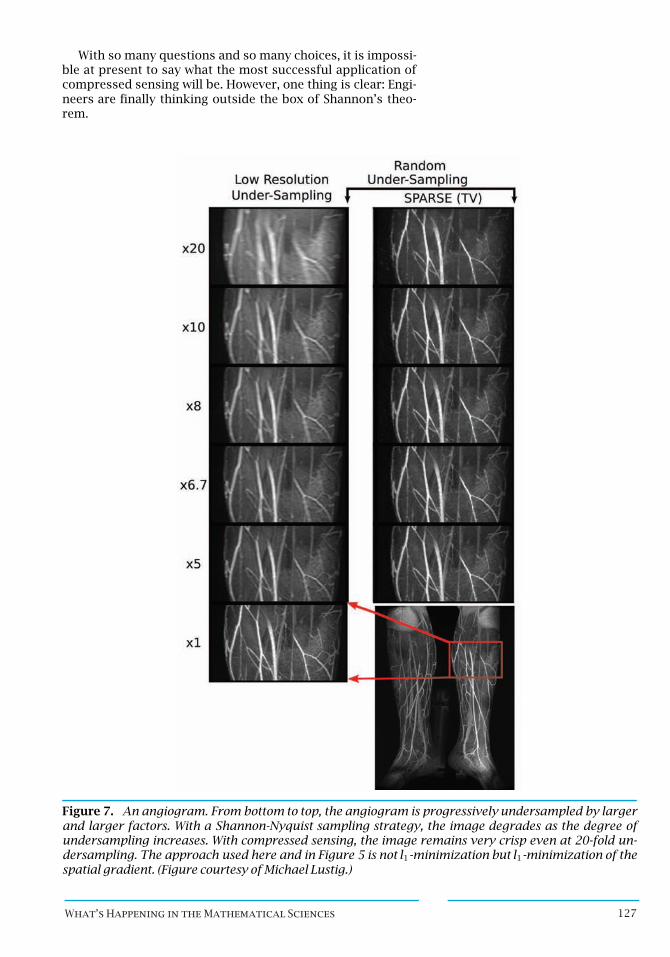
Finally, compressedsensing may find some medical applica-tions—which would be only natural because the theory was di-rectly inspired by a problem in magnetic resonance imaging.MRI scanners have traditionally been limited to imaging staticstructures over a short period of time, and the patient has beeninstructed to hold his or her breath. But now, by treating theimage as a sparse signal in space and time, MRI scanners havebegun to overcome these limitations and produce images, forexample, of a beating heart. Figure 7 shows how a sparse recon-struction algorithm can provide a sharp image of the arteriesin a patient’s leg even with as many as 20 times less data than aconventional angiogram.

One hurdle that compressed sensing may have to overcomeis how to develop practical “incoherent sensors.” A single mea-surement, in compressed sensing, is an inner product of theincoming compressible signal with a random, noisy test signal.Baraniuk’s single-pixel camera accomplishes the inner prod-uct by using mirrors to deflect certain parts of the light beamtoward the sensor, while deflecting other parts away. In real ap-plications, if the hardware that performs the incoherent mea-surements is more expensive than the array of sensors that itis designed to replace, then the economic case for compressedsensing will disappear.


With so many questions and so many choices, it is impossi-ble at present to say what the most successful application ofcompressed sensing will be. However, one thing is clear: Engi-neers are finally thinking outside the box of Shannon’s theo-rem.

Figure 7. An angiogram. From bottom to top, the angiogram is progressively undersampled by largerand larger factors. With a Shannon-Nyquist sampling strategy, the image degrades as the degree ofundersampling increases. With compressed sensing, the image remains very crisp even at 20-fold un-dersampling. The approach used here and in Figure 5 is not l1-minimization but l1-minimization of thespatial gradient. (Figure courtesy of Michael Lustig.)


signal is enough. a photograph taken by the “single-pixel camera” builtby richard baraniuk and...

Documents