signal in noise - confex filescott zrebiec / signal in noise 2 outline smoothing methods allow the...

Scott Zrebiec / Signal in Noise 1

Signal in Noise

Scott Zrebiec, Ph.D.

LexisNexis Insurance Data Services, Modeling & Analytics

April, 2014


Outline

Smoothing methods allow the creation of extremely

predictive data out of signal that would otherwise

be hidden in the noise.

1. Hierarchical Credibility

2. Mathematical Approaches

3. Spatial smoothing approaches

Methods:

Noisy & Accurate Accurate & Precise


Accuracy vs Precision

X

X

X

X

X

X

X

XXX

XX

Goal: Accurate and Precise!

Perfect Accuracy Biased but Precise


Hierarchical Credibility Theory

-Practical way to improve data

-Works with any hierarchy

-Great performance


1. Credibility

Simplistic view of Credibility:

• Employs some independence assumption

• Uses a simple hierarchy:

Large “Credible” sample

Similar “non-Credible” sample

The strength of credibility is in its practicality:

reducing variance of estimates.


1. Miscellaneous Rant

Theorem: (“Central Lie of Mathematics”).

If {X j} is a sequence of i.i.d. random

variables,

and if E[X j] = mu < ∞,

and if 0< Var[X j] = 𝜎^2 < ∞,

Then lim𝑛→∞𝑛

(𝑋𝑗−𝜇 )

𝑛→ 𝑁(0, 𝜎)𝑛

𝑗=1

Observation: Independence is not in general true.


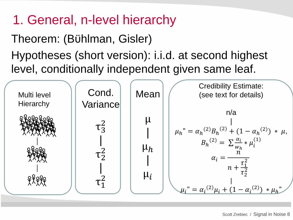
1. General, n-level hierarchy

Theorem: (Bϋhlman, Gisler)

Hypotheses (short version): i.i.d. at second highest

level, conditionally independent given same leaf.

Multi level

Hierarchy

Cond.

Variance

τ32

|

τ22

|

τ12

Mean

µ |

µℎ |

µ𝑖

Credibility Estimate:

(see text for details)

n/a

|

𝜇ℎ" = 𝛼ℎ(2)𝐵ℎ

(2) + (1 − 𝛼ℎ(2)) ∗ 𝜇,

𝐵ℎ(2) =

𝛼𝑖

𝑤ℎ∗ 𝜇𝑖(1)

𝛼𝑖 =𝑛

𝑛 +𝜏12

𝜏22

|

𝜇𝑖" = 𝛼𝑖(2)𝜇𝑖 + (1 − 𝛼𝑖

(2)) ∗ 𝜇ℎ"


1. A Noisy Accurate Data Element

Consider by peril, regional loss statistics

• 𝐹𝑟𝑒𝑞𝑢𝑒𝑛𝑐𝑦 =𝐶𝑙𝑎𝑖𝑚 𝐶𝑜𝑢𝑛𝑡𝑠

𝐸𝑎𝑟𝑛𝑒𝑑 𝐸𝑥𝑝𝑜𝑠𝑢𝑟𝑒

• 𝑆𝑒𝑣𝑒𝑟𝑖𝑡𝑦 =𝐿𝑜𝑠𝑠 𝐴𝑚𝑜𝑢𝑛𝑡𝑠

𝐶𝑙𝑎𝑖𝑚 𝐶𝑜𝑢𝑛𝑡𝑠

• 𝐿𝑜𝑠𝑠 𝐶𝑜𝑠𝑡 =𝐿𝑜𝑠𝑠 𝑃𝑎𝑖𝑑

𝐶𝑙𝑎𝑖𝑚 𝐶𝑜𝑢𝑛𝑡𝑠

Statistics are easy to compute, and accurate.

At the finer levels they are too noisy to be useful.


1. Credibility Smoothing Results

Weighted estimates are stable and accurate

Texas Texas

Precision gained by weighting with similar data.

-6

-5

-4

-3

-2

-1

0

-3 -2 -1 0 1 2 3

-6

-5

-4

-3

-2

-1

0

-2 -1 0 1 2 3

Retro Geoblock Group

Wind Claim Frequency Smoothed Retro Wind Claim Frequency Log o

f W

ind C

laim

Fre

q.

Log o

f W

ind C

laim

Fre

q.


Mathematical Smoothing Techniques

-Identify similarity

-Smooth IDW Average

-Creates new data


2. Metrics Identify Where to Weight

Metrics quantify similarity/distance between

objects.

Lots of types of metrics:

• “Euclidean” Distance

• Distance between houses using characteristics

• Distance between areas using statistics


2. How to Creating Metrics

Creation of a metric/component metric

• Transform to segment

– e.g. Year built is great at segmenting post 1960

– 𝐷𝑖𝑠𝑡𝑎𝑛𝑐𝑒 𝑌𝐵 𝑏𝑒𝑡𝑤𝑒𝑒𝑛 2 𝑝𝑟𝑜𝑝.= Δ 𝑅𝑒𝑠𝑐𝑎𝑙𝑒𝑑 𝑌𝑒𝑎𝑟 𝐵𝑢𝑖𝑙𝑡

• Rescale/ data to be comparable

Combine component metrics using 𝐿𝑝 metrics

• 𝐻. 𝐷𝑖𝑠𝑡𝑎𝑛𝑐𝑒 = 𝑐𝑗 ∗ 𝐷𝑖𝑠𝑡𝑎𝑛𝑐𝑒 𝑓𝑜𝑟 𝐶ℎ𝑎𝑟𝑎𝑐𝑡𝑒𝑟𝑖𝑠𝑡𝑖𝑐 𝑗2

Optimize 𝑐𝑗 and transformation based on needs.


2. IDW averages

IDW averaging smooths data by putting the most

weight on the most similar data

• 𝐼𝐷𝑊 𝐴𝑣𝑔 𝑜𝑓 𝑋 𝑓𝑜𝑟 𝑂𝑏𝑠 𝑗 = 𝑤𝑖∗𝑋𝑖 𝑤𝑖

• 𝑤𝑖,𝑗 =1

𝐷𝑖𝑠𝑡𝑎𝑛𝑐𝑒 𝑓𝑟𝑜𝑚 𝑜𝑏𝑠.𝑗 𝑡𝑜 𝑜𝑏𝑠 𝑖

Uses: Weather data, Property Characteristics, high

dimensional metric space.


2. Example-Identifying Comps

Property Base Best Match Next Best

Match Worst Match

Value 65,900 65,800 NA 350,000

Baths 1 1 1 3

Area NA NA 1124 NA

Story 1 1 1 2

Garage Carport Carport Carport Attached

A.D. 0.0 0.6 0.6 16

Goal: provide a default value for missing data

Adaptive Distance: Measures similarity of two properties using:

“Distance” between two properties based on 10 characteristics

Uses the data that is present


2. IDW Averaging Results

Imputation: Accurate Default Values

• Results are accurate and precise

• Outliers are slightly biased towards the mean

Actual Age (Grouped)

Imputed

Age


Spatial Smoothing Approaches

-Point Region Observations

-Kernel and Kriging Methods

-Results


3. Point data

Source: NOAA Storm Prediction Center; http://www.spc.noaa.gov/climo/online/monthly/2012_annual_summary.html#

http://www.spc.noaa.gov/climo/online/monthly/2012_annual_summary.html














3. Kernel Smoothing

Point data is assigned to regions using Kernel

smoothing

𝐻𝑎𝑖𝑙 𝑅𝑖𝑠𝑘 𝑎𝑡 𝑥 = 𝐾𝜆(𝑥, 𝑦)

{𝑦}

Where 𝑓(𝑥) = 𝐾𝜆(𝑥, 𝑦) is the pdf at x for a Random

variable, e.g. Uniform, with μ=y and σ = 𝜆.

Even simpler interpretation: Number of Storm events in

X –miles in the past Y years

Issues: observational bias, boundary effect, choice of λ


3. Kernel Smoothing Results

-9

-8

-7

-6

-5

-4

-3

-2

-1

0

-4 -3 -2 -1 0 1 2

log

of

Hail

Cla

im F

req

uen

cy

Renormalized log transformed Kernel Smoothed Hail probability

U.S. Sample


3. Kriging

Observation: Adjacent points have correlated

geographic data.

Kriging:

• Assumes a Gaussian field:

– Each position associated with random variable

– Spatial correlation

– Either interpolation or statistical fit

• Smoothed average of nearby points.

• Produces “similar” results to kernel approaches


3. Map-Wind Storm Probability:


3. Kriging Results

-8

-7

-6

-5

-4

-3

-2

-1

0

-2.5 -2 -1.5 -1 -0.5 0 0.5 1 1.5 2

Lo

g o

f H

ail

Cla

im F

req

uen

cy

Renormalized Log of Large Hail Storm Prob.

U.S. Sample


3. Good Data gives good models:

Houses

• in areas with many historic Wind & Hail Storms/Claim activity

• That have risky property characteristics

Tend to have high hail losses.

0.0%

1.0%

2.0%

3.0%

0

100

200

300

400

500

600

700

800

1 3 5 7 9

11

13

15

17

19

21

23

25

27

29

31

33

35

37

39

41

43

45

47

49

51

53

55

57

59

61

63

65

67

69

71

73

75

77

79

81

83

85

87

89

91

93

95

97

99

Exp

osu

re

Av

era

ge W

ind

Paid

Lo

ss

Wind Index 1-100

TX Non-Cat Wind Wind Paid Loss Cost

Exposure


Conclusions

Smoothing methods create good data out of

accurate garbage.

Consider smoothing methods whenever:

• Data is very predictive but very noisy

• Data is associated with a different class of objects

• Data is missing


Thank you

Scott Zrebiec, Ph.D.

Manager Statistical Modeling

LexisNexis Risk Solutions

[email protected]

mailto:[email protected]

mailto:[email protected]


References

• H. Bϋhlman, A. Gisler, A course in Credibility

theory and its applications, Springer, 2008.

• T. Hastie, R. Tibshirani, J. Friedmann Elements

of Statistical Learning, Springer, 2001.

• R. Bivand, E. Pebesma, V. Gomez-Rubio,

Applied Spatial Data Analysis with R, Springer,

2008.

signal in noise - confex filescott zrebiec / signal in noise 2 outline smoothing methods allow the...

Documents