signal analysis and performance evaluation of a vehicle ... · parameter modeling in...
TRANSCRIPT

August 25, 2010 21:25 WSPC/WS-IJWMIP 2011-1-6
International Journal of Wavelets, Multiresolution and Information Processingc© World Scientific Publishing Company
Signal Analysis and Performance Evaluation of a Vehicle Crash Test
with a Fixed Safety Barrier Based on Haar Wavelets
Hamid Reza Karimi∗and Kjell G. Robbersmyr
Department of Engineering, Faculty of Engineering and Science, University of Agder
N-4898 Grimstad, Norway
[email protected]; [email protected]
Received 3 November 2009Revised 20 March 2010
This paper deals with the wavelet-based performance analysis of the safety barrier foruse in a full-scale test. The test involves a vehicle, a Ford Fiesta, which strikes thesafety barrier at a prescribed angle and speed. The vehicle speed before the collision wasmeasured. Vehicle accelerations in three directions at the centre of gravity were measured
during the collision. The yaw rate was measured with a gyro meter. Using normal speedand high-speed video cameras, the behavior of the safety barrier and the test vehicleduring the collision was recorded. Based upon the results obtained, the tested safetybarrier, has proved to satisfy the requirements for an impact severity level. By taking
into account the Haar wavelets, the property of integral operational matrix is utilized tofind an algebraic representation form for calculate of wavelet coefficients of accelerationsignals. It is shown that Haar wavelets can construct the acceleration signals well.
Keywords: Wavelet; Traffic safety; Safety barrier; Collision; Acceptance criteria.
AMS Subject Classification: 42C40, 35G20, 65M70
1. Introduction
Restraint systems are safety devices that are designed to assist in restraining the
occupant in the seating position, and help reduce the risk of occupant contact with
the vehicle interior, thus helping reduce the risk of injury in a vehicular crash event.
In todays quest for continued improvement in automotive safety, various restraint
systems have been developed to provide occupant protection in a wide variety of
crash environments under different directions and conditions. It is extremely diffi-
cult to present rigorous mathematical treatments to cover occupant kinematics in
complicated real world situations 5’40.
Occupant safety during a crash is an important consideration in the design
of automobiles. The crash performance of an automobile largely depends on the
ability of its structure to absorb the kinetic energy and to maintain the integrity
∗Corresponding author. Tel: +47-3723-3259; Fax: +47-3723-3001; E-mail: [email protected]
1

August 25, 2010 21:25 WSPC/WS-IJWMIP 2011-1-6
2 H.R. Karimi and K.G. Robbersmyr
of the occupant compartment. To verify the crash performance of automobiles,
extensive testing as well as analysis are needed during the early stages of design.
Various types of full car and component level tests are performed to ensure the
structural performance of an automobile during an accident. Two full car tests
required by the U.S. National Highway Traffic Safety Administration (NHTSA)
are the frontal impact and side impact. In the frontal impact test, the test vehicle
hits a rigid wall and the injury is measured in terms of accelerations at various
locations (such as head, chest, etc.), using dummies as human surrogates. The
occupant protection can be improved by designing the front end in structure to
minimize deceleration of the occupant while maintaining the structural integrity of
the occupant compartment. In the test procedure for a side impact, a stationary
vehicle is struck by a specially designed barrier called an MDB (moving deformable
barrier). Two devices representing occupants (SIDs or side impact dummies) are
located in the front and rear seat of the struck side of the vehicle. The injury is
measured in terms of the peak accelerations of a SID’s chest and pelvis. The injury
protection for the occupant can be improved by making the car structure stiffer
while making the car interior that comes into contact with the occupant softer13.
In the last ten years, emphasis on the use of analytical tools in design and
crash performance has increased as a result of the rising cost of building prototypes
and the shortening of product development cycles. Currently, lumped parameter
modeling (LPM) and finite element modeling (FEM) are the most popular analytical
tools in modeling the crash performance of an automobile2’6. The use of lumped
parameter modeling in crash-worthiness began in the aerospace industry and was
gradually extended to the auto industry. The first successful lumped parameter
model for the frontal crash of an automobile was developed by Kamal20. From then
on this technique was extensively used throughout the auto industry for various car
models. In a typical lumped parameter model, used for a frontal crash, the vehicle
can be represented as a combination of masses, springs and dampers. The dynamic
relationships among the lumped parameters are established using Newton’s laws
of motion and then the set of differential equations are solved using numerical
integration techniques. The major advantage of this technique is the simplicity
of modeling and the low demand on computer resources. The problem with this
method is obtaining the values for the lumped parameters, e.g. mass, stiffness, and
damping. The current approach is to crush the structural components using a static
crusher to get force deflection characteristics. The mass is lumped based on the
experience and judgment of the analyst. However, because of improper boundary
conditions during the component test, it has been observed in many cases that
the crush mode for a particular component during the static component crush is
quite different from that seen in a full car test. Usually complicated fixtures and
additional parts are attached to the component being tested to achieve the proper
end conditions. This adds complexity and cost to the component crush test. Since
the early 60s, the finite element method (FEM) has been used extensively for linear
stress, deflection and vibration analysis. However, its use in crashworthiness analysis

August 25, 2010 21:25 WSPC/WS-IJWMIP 2011-1-6
Signal Analysis and Performance Evaluation of a Vehicle Crash Test 3
was very limited until a few years ago. The availability of general purpose crash
simulation codes like DYNA3D and PAMCRASH, an increased understanding of
the plasticity behavior of sheet metal, and increased availability of the computer
resources have increased the use of finite element technique in crash simulation
during the last few years16’21’32’38. The major advantage of an FEM model is
its capability to represent geometrical and material details of the structure. The
major disadvantage of FE models is cost and time. To obtain good correlation of
an FEM stimulation with test measurements, extensive representation of the major
mechanisms in the crash event is required. This increases costs and the time required
for modeling and analysis.
On the other hand, in recent years, wavelet transform as a new technique for
time domain simulations based on the time-frequency localization, or multiresolu-
tion property, has been developed into a more and more complete system. This
transform found great success in practical engineering problems, such as signal pro-
cessing, pattern recognition and computational graphics14’18’35. Recently, some of
the attempts are made in solving surface integral equations, improving the finite
difference time domain method, solving linear differential equations and nonlin-
ear partial differential equations and modeling nonlinear semiconductor devices.
Several articles have been published recently in the fields of applied mathematics
and physics that present wavelet based methods for resolution of (partial differen-
tial equations) PDEs1’4. These are classified as collocation methods or Galerkin
methods3’7’10’15’17’19’22’23’24’25’26’27’28’29’30’31’37. The approximation of general
continuous functions by wavelets is very useful for system modeling and identifica-
tion. In recent years, the analytical study of adaptive nonlinear control systems using
universal function approximators has received much attention. Recently, the paper
Onchis and Suarez Sanchez34 studied the spectral decomposition and the adaptive
analysis of data coming from car crash simulations. The mathematical ingredient
of the proposed signal processing technique is the flexible Gabor-wavelet transform
or the α-transform that reliably detects both high and low frequency components
of such complicated short-time signals. We go from the functional treatment of this
wavelet-type transform to its numerical implementation and we show how it can
be used as an improved tool for spectral investigations compared to the short-time
Fourier transform or the classical wavelet transform.
The present work intends to, emphasizing the advantages of wavelets, analyze
performance of the safety barrier for use in a full-scale test. Also in this article, we
use the Haar wavelets to calculate wavelet coefficients. The test involves a vehicle,
a Ford Fiesta, which strikes the safety barrier at a prescribed angle and speed.
The vehicle speed before the collision was measured. Vehicle accelerations in three
directions at the centre of gravity were measured during the collision. The yaw
rate was measured with a gyro meter. Using normal speed and high-speed video
cameras, the behavior of the safety barrier and the test vehicle during the collision
was recorded. Based upon the results obtained, the tested safety barrier, has proved
to satisfy the requirements for an impact severity level. By taking into account the
August 25, 2010 21:25 WSPC/WS-IJWMIP 2011-1-6
4 H.R. Karimi and K.G. Robbersmyr
Haar wavelets, the property of integral operational matrix is utilized to find an
algebraic representation form for calculate of wavelet coefficients of acceleration
signals. It is shown that Haar wavelets can construct the acceleration signals well.
This paper is organized as follows. Section 2 describes the wavelet properties.
Vehicle kinematics in a fixed barrier impact, including the vehicle dimensions and
position of the center of gravity, are summarize in Section 3. Instrumentation during
the test is given in Section 4. Section 5 proposes wavelet-based analysis of the
measured signals. Finally, Section 6 summarizes the paper.
2. Orthogonal families of Wavelets
Wavelets are a relatively new mathematical concept, introduced at the end of the
1980s11’12’33. The term ”wavelet” is used in general to describe a function that
features compact support. This means that the function is located spatially, only
being different from zero in a finite interval.
The great advantage of this type of function, compared to the conventional
functions used in data representation, is that different resolution levels can be used
to describe distinct space or time regions. This feature is quite useful in signal,
sound, and image compression algorithms. When a data set goes through a wavelet
transformation, it is decomposed into two types of coefficients: one represents gen-
eral features (scaling function coefficients) and another describes localized features
(wavelet coefficients). In order to perform data compression, the wavelet coefficients
corresponding to regions in space of less importance are partially rejected. Then,
when the function is reconstructed, high resolution is maintained only in the rele-
vant regions. This localized resolution feature does not exist in plane waves, which
have constant resolution throughout the entire domain.
Two functions, the mother scaling function, φ , and the mother wavelet, ψ ,
characterize each orthogonal family. These are defined by the following recursive
relations
φ(x) =√2
m∑
j=−m
hjφ(2x− j), ψ(x) =√2
m∑
j=−m
gjφ(2x− j). (2.1)
where hj and gj are the filters that characterize the family of degreem . These filters
must satisfy orthogonality and symmetry relations. Due to the choice of the filters
hj and gj , the dilations and translations of the mother scaling function, φjk(x) , and
the mother wavelet, ψjk(x) , form an orthogonal basis of L2(R). This property has an
important consequence: any continuous function, f(x) can be uniquely projected
in this orthogonal basis and expressed as, for example, a linear combination of
functions ψjk .
f(x) =∑
j∈Z
∑
k∈Z
djkψjk(x) . (2.2)
where djk =∫∞
−∞f(x)ψj
k(x)dx.

August 25, 2010 21:25 WSPC/WS-IJWMIP 2011-1-6
Signal Analysis and Performance Evaluation of a Vehicle Crash Test 5
2.1. Expansion of a continuous function
Regarding to multiresolution analysis, the expansion of a continuous function in
wavelet theory can be performed according to two representations. The first scaling
function representation involves only the scaling functions; the second, wavelet rep-
resentation, involves both wavelets and scaling functions. The representations are
equivalent and need the exact same number of coefficients. One can move from one
representation to the other by using a process designated as wavelet transform39.
The scaling function representation is given by
f(x) =
2Jmax∑
k=0
sJmax
k φJmax
k (x) . (2.3)
where sJmax
k =∫f(x)φJmax
k (x)dx is the scaling function coefficient, Jmax is the
maximum resolution level, and k represents the spatial location. The wavelet rep-
resentation is given by
f(x) =2Jmin∑
k=0
sJmin
k φJmin
k (x) +
Jmax−1∑
j=Jmin
2j∑
k=0
djkψjk(x) . (2.4)
where d is the wavelet coefficient and Jmin is the minimum resolution level,
djk =
∫∞
−∞
f(x)ψjk(x)dx, sJmin
k =
∫∞
−∞
f(x)φjk(x)dx. (2.5)
Integrations have to be performed in order to compute the expansion coefficients.
Several methods have been proposed in the literature for accomplishing this, starting
from a function’s discrete values. These methods necessarily introduce a certain
approximation error and increase the complexity of the problem, namely in the
solution of PDEs. There is, however, a wavelet family for which these integrations
are exact: the interpolating wavelets.
2.2. Haar Wavelet
The oldest and most basic of the wavelet systems is named Haar wavelets28 which
is a group of square waves with magnitudes of ±1 in certain intervals and zero
elsewhere,in other words,
ψ(t) =
1 if 0 ≤ t < 12 ,
−1 if 12 ≤ t < 1,
0 otherwise
(2.6)
The normalized scaling function is also defined as φ(t) = 1 for 0 ≤ t < 1 and
zero elsewhere. Just these zeros make the Haar transform faster than other square
functions such as Walsh function9. We can easily see that the φ(.) and ψ(.) are com-
pactly supported, they give a local description, at different scales j, of the considered
function.
August 25, 2010 21:25 WSPC/WS-IJWMIP 2011-1-6
6 H.R. Karimi and K.G. Robbersmyr
The wavelet series representation of the one-dimensional function y(t) in terms
of an orthonormal basis in the interval [0, 1) is given by
y(t) =
∞∑
i=0
ai ψi(t) (2.7)
where ψi(t) = ψ(2jt− k) for i ≥ 1 and we write i = 2j + k for j ≥ 0 and 0 ≤ k < 2j
and also defined ψ0(t) = φ(t). Since it is not realistic to use an infinite number of
wavelets to represent the function y(t), (2.7) will be terminated at finite terms and
we consider the following wavelet representation y(t) of the function y(t):
y(t) =
m−1∑
i=0
ai ψi(t) := aTΨm(t), (2.8)
where a :=[a0 a1 . . . am−1
]Tand Ψm(t) := [ψ0(t)ψ1(t) . . . ψm−1(t)]
T for m = 2j
and the Haar coefficients ai are determined as
ai = 2j∫ 1
0
y(t)ψi(t) dt. (2.9)
The approximation error Ξy(m) := y(t) − y(t) depends on the resolution m. For
example, at resolution scale j = 3 , the eight Haar functions can be represented as
H8 =
ψ0(t)
ψ1(t)
ψ2(t)
ψ3(t)
ψ4(t)
ψ5(t)
ψ6(t)
ψ7(t)
=
1 1 1 1 1 1 1 1
1 1 1 1 −1 −1 −1 −1
1 1 −1 −1 0 0 0 0
0 0 0 0 1 1 −1 −1
1 −1 0 0 0 0 0 0
0 0 1 −1 0 0 0 0
0 0 0 0 1 −1 0 0
0 0 0 0 0 0 1 −1
, (2.10)
where the eight columns of the matrix represent the values of ψi(t) within the eight
time intervals. In (2.10) the number of rows denotes the order of the Haar function.
Generally, the matrix Hm can be represented as
Hm :=[Ψm(t0) Ψm(t1) . . . Ψm(tm−1)
], (2.11)
where im
≤ ti <i+1m
and using (2.8), we get[y(t0) y(t1) . . . y(tm−1)
]= aTHm. (2.12)
For further information see the references8’28’29’30.
2.3. Integral Operation Matrix
In the wavelet analysis of dynamical systems, we consider a continuous operator O
on the L2(ℜ), then the corresponding discretized operator in the wavelet domain
at resolution m is defined as28
Om
= Tm OTm (2.13)
August 25, 2010 21:25 WSPC/WS-IJWMIP 2011-1-6
Signal Analysis and Performance Evaluation of a Vehicle Crash Test 7
where Tm is the projection operator on a wavelet basis of proposed resolution. Hence
to apply Om
to a function y(t) means that the result is an approximation (in the
multiresolution meaning) of O y(t) and it holds that
limm→∞
‖Omy − O y‖2 = 0, (2.14)
where the operator Om
can be represented by a matrix Pm.
In this paper, the operator O is considered as integration, so the corresponding
matrix Pm =<∫ t
0Ψm(τ) dτ,Ψm(t) >=
∫ 1
0
∫ t
0Ψm(τ) dτ ΨT
m(t) dt represents the in-
tegral operator for wavelets on the interval at the resolution m. Hence the wavelet
integral operational matrix Pm is obtained by∫ t
0
Ψm(τ) dτ = PmΨm(t). (2.15)
For Haar function (2.6), the square matrix Pm satisfies the following recursive
formula8’28’29’30:
Pm =1
2m
[
2mPm2−Hm
2
H−1m2
0
]
(2.16)
with P1 = 12 and H−1
m = 1mHT
m diagonal(r) where Hm defined in (2.11) and r :=
(1, 1, 2, 2, 4, 4, 4, 4, . . . , (m
2), (
m
2), . . . , (
m
2)
︸ ︷︷ ︸
(m2)elements
)T for m > 2.
3. Vehicle kinematics in a fixed barrier impact
The first and second integrals of the vehicle deceleration, a(t), are shown below. The
initial velocity and initial displacements of the vehicle are v0 and x0, respectively.
a =dv
dt, dv = a dt,
∫ v
v0
dv =
∫ t
0
a dt, v = v0 +
∫ t
0
a dt (3.1)
x = x0 +
∫ t
0
(
v0 +
∫ t
0
a dt
)
dt, (3.2)
In the fixed barrier test, vehicle speed is reduced (velocity decreases) by the struc-
tural collapse, therefore, the vehicle experiences a deceleration in the forward direc-
tion. To study the effect of vehicle deceleration on occupant-restraint performance
in a real test, the performance of the safety barrier was determined by performing
a full-scale test at Lista Airport36. The test involves a vehicle, a Ford Fiesta, which
strikes the safety barrier at a prescribed angle and speed. The vehicle speed before
the collision was measured. Vehicle accelerations in three directions at the centre
of gravity were measured during the collisison. The yaw rate was measured with
a gyro meter. Using normal speed and high-speed video cameras, the behaviour of
the safety barrier and the test vehicle during the collision was recorded.

August 25, 2010 21:25 WSPC/WS-IJWMIP 2011-1-6
8 H.R. Karimi and K.G. Robbersmyr
3.1. Vehicle dimensions
Figure 1 shows the characteristic parameters of the vehicle, and these parameters
are listed in Table 1.
Table 1. Vehicle dimensions in [m].
Wheel Wheel Frontal Rear
Width Length Height track base overhang overhang
1.58 3.56 1.36 1.42 2.28 0.63 0.65
Fig. 1. Vehicle dimensions.
3.2. The position of the center of gravity
To determine the position of the center of gravity each test vehicle was first weighed
in a horizontal position using 4 load cells. Then the vehicle was tilted by lifting the
front of the vehicle. In both positions the following parameters were recorded:
• m1 : wheel load, front left
• m2: wheel load, front right

August 25, 2010 21:25 WSPC/WS-IJWMIP 2011-1-6
Signal Analysis and Performance Evaluation of a Vehicle Crash Test 9
• m3 : wheel load, rear left
• m4 : wheel load, rear right
• mv : total load
• θ : tilted angle
• l : wheel base
• d : distance across the median plane between the vertical slings from the lift
brackets at the wheel centers and the load cells.
The horizontal distance between the center of gravity and the front axle center-
line, i.e. Longitudinal location, is defined as follows:
CGX = (m3 +m4
mv
)l
and Laterally location is the horizontal distance between the longitudinal median
plane of the vehicle and the center of gravity (positive to the left) which is defined
as
CGY = (m1 +m3 − (m2 +m4)
mv
)d
2
Also, location of the center of gravity above a plane through the wheel centers is
CGZ = (m1 +m2 −mf )
mv tanθ)l
where
• mf : front mass in tilted position
• mb : rear mass in tilted position
Table 2. shows the measured parameters to calculate the center of gravity. The
position of the centre of gravity for the test vehicle is measured and the result is
listed in Table 3.
Table 2. Measured parameters.
m1 [kg] m2 [kg] m3 [kg] m4 [kg] mv [kg] mf [kg] mb [kg] d [m] l [m] θ [deg]
235 245 182 157 819 443 376 1.71 2.28 22.7
Table 3. The position of the centre of gravity.
Longitudinal location Lateral location HeightCGX [m] CGY [m] CGZ [m]
0.94 0.02 0.50

August 25, 2010 21:25 WSPC/WS-IJWMIP 2011-1-6
10 H.R. Karimi and K.G. Robbersmyr
4. Instrumentation
During the test, the following data should be determined:
• Acceleration in three directions during and after the impact
• Velocity 6 m before the impact point
The damage should be visualized by means of:
• Still pictures
• High speed video film
The observations should establish the base for a performance evaluation. Eight video
cameras were used for documentation purposes. These cameras are placed relative
to the test item as shown in Figure 1. Two 3-D accelerometers were mounted on
a steel bracket close to the vehicles centre of gravity. This bracket is fastened by
screws to the vehicle chassis. The accelerometer from which the measurements are
recorded is a piezoresistive triaxial sensor with accelerometer range: ±1500g. The
yaw rate was measured with a gyro instrument with which it is possible to record
1o/msec. Figures 2-4 show the measurements of the 3-D accelerometer in x−,y−and z− directions.
Data from the sensors was fed to an eight channel data logger. The logger has a
sampling rate of 10 kHz. The memory is able to store 6,5 sec of data per channel.
The impact velocity of the test vehicle was measured with an equipment using two
infrared beams. The equipment is produced by Alge Timing and is using Timer S4
and photo cell RL S1c. On the test vehicle a plate with a vertical egde was mounted
on the left side of the front bumper. This vertical egde will cut the reflected infrared
beams in the timing equipment and thereby give signals for calculation of the speed.
The test vehicle was steered using a guide bolt which followed a guide track in the
concrete runway. About 7m before the test vehicle hit the test item the guide bolt
was released. Vehicle accelerations at the centre of gravity was measured, and also
the yaw rate of the vehicle. These measurements make it possible to calculate the
Acceleration Severity Index (ASI), the Theoretical Head Impact Velocity (THIV),
the Post-impact Head Deceleration (PHD) value and the yaw rate. The impact
speed of the test vehicle was determined. The ASI-, the THIV- and the PHD-values
are calculated according to EN 1317-1 clause 6 and clause 7, and the results are
shown in Table 4. Using normal speed- and high-speed video cameras, the behavior
of the safety barrier and test vehicle during the collision was recorded, see Figures
5-6. The value of ASI corresponds to the requirement for impact severity level B.
The THIV- and PHD-values are below the limiting values.
5. Wavelet-Based Signal Analysis
This section attempts to show the effectiveness of the wavelet technique to represent
the measured signals of the test. By choosing the resolution level j = 7 (or m =
28) and expansion of the acceleration signal x(t), v(t), a(t) in (3.1)-(3.2) by Haar

August 25, 2010 21:25 WSPC/WS-IJWMIP 2011-1-6
Signal Analysis and Performance Evaluation of a Vehicle Crash Test 11
Table 4. The calcula-
tion results.
ASI THIV PHD
1.28 29.9 7.8
0 0.5 1 1.5 2 2.5 3 3.5
x 104
−40
−30
−20
−10
0
10
20
t[ms]
a x [g]
Fig. 2. Acceleration signal in x- direction.
0 0.5 1 1.5 2 2.5 3 3.5
x 104
−40
−30
−20
−10
0
10
20
30
40
t[ms]
a y [g]
Fig. 3. Acceleration signal in y- direction.
wavelets, we have x(t) = XΨm(t), v(t) = VΨm(t) and a(t) = AΨm(t), in which
the row vectors X,V,A ∈ ℜ1×m are the Haar wavelet coefficient vectors. Utilizing
the property of the Haar integral operation matrix, Haar wavelet representation of
equations (3.1)-(3.2) are, respectively,
VΨm(t) = V0Ψm(t) +
∫ t
0
AΨm(τ) dτ = V0Ψm(t) +APmΨm(t) (5.1)

August 25, 2010 21:25 WSPC/WS-IJWMIP 2011-1-6
12 H.R. Karimi and K.G. Robbersmyr
0 0.5 1 1.5 2 2.5 3 3.5
x 104
−30
−20
−10
0
10
20
30
t[ms]
a z [g]
Fig. 4. Acceleration signal in z- direction.
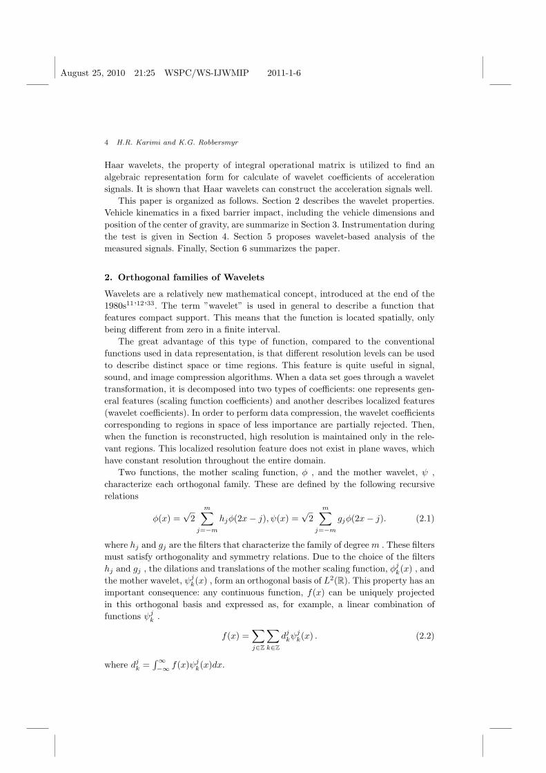
Fig. 5. The situation recorded at the first contact.
and
XΨm(t) = X0Ψm(t) +
∫ t
0
V0Ψm(τ)dτ +
∫ t
0
∫ t
0
AΨm(τ) dτ dt,
= X0Ψm(t) + V0PmΨm(t) +AP 2mΨm(t) (5.2)
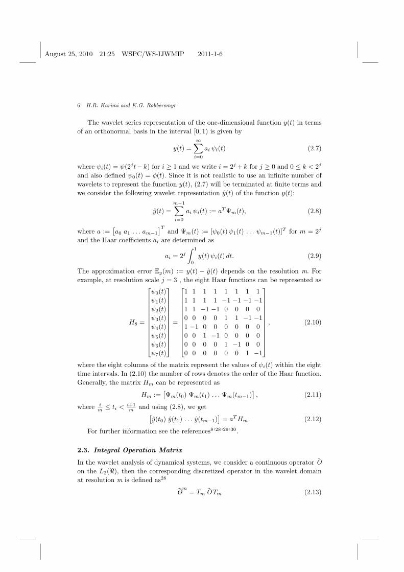
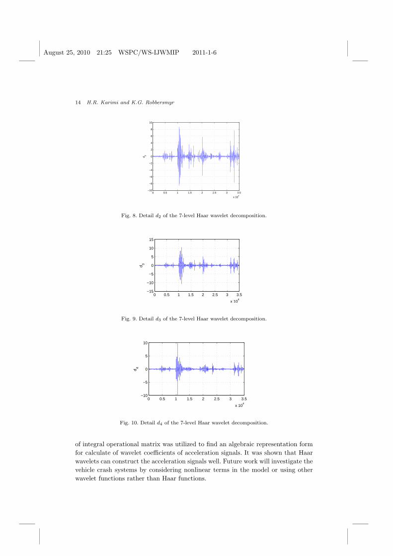
Constituting the Haar wavelet properties in (5.1)-(5.2), a seven-level wavelet de-
composition of the measured x-acceleration signal (ax) is performed and the results,
i.e. the approximation signal (a7) and the detail signals (d1-d7) at the resolution
level 7, are depicted in Figures 7-14. One advantage of using these multilevel decom-
position is that we can zoom in easily on any part of the signals and examine it in
greater detail. Using the approximation signal (a1) and the detail signal (d1) at the
resolution level 1 by Haar wavelets, Figure 15 compares the constructed signal ax(t)
(solid line) with the real signal (dashed line). It is noted that the approximation
error between those curves in Figure 15 is decreasing when the resolution level j
August 25, 2010 21:25 WSPC/WS-IJWMIP 2011-1-6
Signal Analysis and Performance Evaluation of a Vehicle Crash Test 13
Fig. 6. The situation recorded 0.148 sec after the impact.
0 0.5 1 1.5 2 2.5 3 3.5
x 104
−10
−5
0
5
10
d 1
Fig. 7. Detail d1 of the 7-level Haar wavelet decomposition.
increases. The results in Figures 7-15 show the capability of the Haar wavelets to
reconstruct the measured signals well.
6. Conclusions
This paper studied the wavelet-based performance analysis of the safety barrier for
use in a full-scale test. The test involves a vehicle, a Ford Fiesta, which strikes
the safety barrier at a prescribed angle and speed. The vehicle speed before the
collision was measured. Vehicle accelerations in three directions at the centre of
gravity were measured during the collision. The yaw rate was measured with a
gyro meter. Using normal speed and high-speed video cameras, the behavior of the
safety barrier and the test vehicle during the collision was recorded. Based upon the
results obtained, the tested safety barrier, has proved to satisfy the requirements
for an impact severity level. By taking into account the Haar wavelets, the property
August 25, 2010 21:25 WSPC/WS-IJWMIP 2011-1-6
14 H.R. Karimi and K.G. Robbersmyr
0 0.5 1 1.5 2 2.5 3 3.5
x 104
−10
−8
−6
−4
−2
0
2
4
6
8
10
d 2
Fig. 8. Detail d2 of the 7-level Haar wavelet decomposition.
0 0.5 1 1.5 2 2.5 3 3.5
x 104
−15
−10
−5
0
5
10
15
d 3
Fig. 9. Detail d3 of the 7-level Haar wavelet decomposition.
0 0.5 1 1.5 2 2.5 3 3.5
x 104
−10
−5
0
5
10
d 4
Fig. 10. Detail d4 of the 7-level Haar wavelet decomposition.
of integral operational matrix was utilized to find an algebraic representation form
for calculate of wavelet coefficients of acceleration signals. It was shown that Haar
wavelets can construct the acceleration signals well. Future work will investigate the
vehicle crash systems by considering nonlinear terms in the model or using other
wavelet functions rather than Haar functions.

August 25, 2010 21:25 WSPC/WS-IJWMIP 2011-1-6
Signal Analysis and Performance Evaluation of a Vehicle Crash Test 15
0 0.5 1 1.5 2 2.5 3 3.5
x 104
−10
−5
0
5
10
d 5
Fig. 11. Detail d5 of the 7-level Haar wavelet decomposition.
0 0.5 1 1.5 2 2.5 3 3.5
x 104
−4
−2
0
2
4
d 6
Fig. 12. Detail d6 of the 7-level Haar wavelet decomposition.
0 0.5 1 1.5 2 2.5 3 3.5
x 104
−10
−5
0
5
10
d 7
Fig. 13. Detail d7 of the 7-level Haar wavelet decomposition.
References
1. E. Bacry, S. Mallat, and G. Papanicolaou, A wavelet based space-time adaptive numer-ical method for partial differential equations, RAIRO Model. Math. Anal. 26 (1992)

August 25, 2010 21:25 WSPC/WS-IJWMIP 2011-1-6
16 H.R. Karimi and K.G. Robbersmyr
0 0.5 1 1.5 2 2.5 3 3.5
x 104
−10
−8
−6
−4
−2
0
2a 7
Approxiation at level 7 (reconstructed)
Fig. 14. The approximation signal a7 of the Haar wavelet decomposition at the resolution level 7.
0 20 40 60 80 100
−0.5
−0.4
−0.3
−0.2
−0.1
0
0.1
0.2
0.3
0.4
0.5
t[ms]
a x [g]
Siganl approximation at level 1
Fig. 15. The constructed signal ax(t) (solid line) at the resolution level 1 with the real signal(dashed line).
793-834.2. T. Belytschko, On computational methods for crashworthiness, Computers and Struc-
ture 42 (1992) 271-279.3. S. Bertoluzza, Adaptive wavelet collocation method for the solution of Burgers equa-
tion, Transp. Theory Stat. Phys., 25 (1996) 339-352.4. G. Beylkin, and J. Keiser, On the Adaptative numerical solution of nonlinear partial
differential equations in wavelets bases, J. Comput. Phys., 132 (1997) 233-259.5. P.D. Bois, C.C. Chou, B.B. Fileta, T.B. Khalil, A.I. King, H.F. Mahmood, H.J. Mertz
and J. Wismans, Vehicle crashworthiness and occupant protection, American Iron andSteel Institute, 2004.
6. M. Borovinsek, M. Vesenjak, M. Ulbin and Z. Ren, ’Simulation of crash test for highcontainment level of road safety barriers’, Engineering Failure Analysis, 14(2007) 1711-1718.
August 25, 2010 21:25 WSPC/WS-IJWMIP 2011-1-6
Signal Analysis and Performance Evaluation of a Vehicle Crash Test 17
7. W. Cai and J.Z. Wang, Adaptive multiresolution collocation methods for initial bound-ary value problems of nonlinear PDEs, J. Numer. Anal., 33(1996) 937-970.
8. C.F. Chen and C.H. Hsiao, ’Haar wavelet method for solving lumped and distributed–parameter systems’, IEE Proc. Control Theory Appl., 144 (1997) 87-94.
9. C.F. Chen and C.H. Hsiao, ’A state-space approach to Walsh series solution of linearsystems’, Int. J. System Sci., 6 (1965) 833-858.
10. W. Dahmen, A. Kunoth, and K. Urban, A wavelet Galerkin method for the stokesequations, Computing, 56 (1996) 259-301.
11. I. Daubechies, ’Orthogonal bases of compactly supported wavelets’ Commun. Pure
Appl. Math., 41 (1988) 909-996.12. I. Daubechies, Ten Lectures on Wavelets, SIAM, Philadelphia, 1992.13. U.N. Gandhi and S.J. Hu, ’Data-based approach in modeling automobile crash’ Int.
J. Impact Engineering, 16 (1995) 95-118.14. A. Graps, An introduction to wavelets, IEEE Comput. Sci. Eng. ,2 (1995) 50-61.15. M. Griebel, and F. Koster, Adaptive Wavelet Solvers for the Unsteady Incompressible
Navier-Stokes Equations, Preprint No. 669, Univ. of Bonn, Bonn, Germany, 2000.16. J. Hallquist and D. Benson, ’DYNA3D–an explicit finite element program for impact
calculations. Crashworthiness and Occupant Protection in Transportation Systems’,The Winter Annual Meeting of ASME, San Francisco, California, 1989.
17. M. Holmstron, Solving hyperbolic PDEs using interpolating wavelets, J. Sci. Comput.
, 21 (1999) 405-420.18. B. Jawerth, and W. Sweldens, An overview of wavelet based multiresolution analyses,
SIAM Re., 36 (1994) 377-412.19. M.K. Kaibara, and S.M. Gomes, Fully adaptive multiresolution scheme for shock com-
putations, Goduno methods: Theory and applications, E.F. Toro, ed., Kluwer AcademicPlenum Publishers, Manchester, U.K. (2001).
20. M. Kamal, Analysis and simulation of vehicle to barrier impact. SAE 700414 (1970).21. T. Khalil and D. Vander Lugt, ’Identification of vehicle front structure crashworthiness
by experiments and finite element analysis. Crashworthiness and occupant protectionin transportation systems’, The Winter Annual Meeting of ASME, San Francisco, Cal-ifornia (1989).
22. A. Karami, H.R. Karimi, B. Moshiri, and P.J. Maralani, ’Wavelet-based adaptive col-location method for the resolution of nonlinear PDEs’ Int. J. Wavelets, Multiresoloution
and Image Processing, 5 (2007) 957-973.23. A. Karami, H.R. Karimi, P.J. Maralani, and B. Moshiri, ’Intelligent optimal control
of robotic manipulators using wavelets’ Int. J. Wavelets, Multiresoloution and Image
Processing, 6 (2008) 575-592.24. H.R. Karimi, B. Lohmann, B. Moshiri, and P.J. Maralani, ’Wavelet-based identifi-
cation and control design for a class of non-linear systems’ Int. J. Wavelets, Mul-
tiresoloution and Image Processing, 4 (2006) 213-226.25. H.R. Karimi, ’A computational method to optimal control problem of time-varying
state-delayed systems by Haar wavelets’, Int. J. Computer Mathematics, 83 (2006)235-246.
26. H.R. Karimi, ’Optimal vibration control of vehicle engine-body system using Haarfunctions’, Int. J. Control, Automation, and Systems, 4 (2006) 714-724.
27. H.R. Karimi, and B. Lohmann, ’Haar wavelet-based robust optimal control for vi-bration reduction of vehicle engine-body system’, Electrical Engineering, 89 (2007)469-478.
28. H.R. Karimi, B. Lohmann, P.J. Maralani and B. Moshiri, ’A computational methodfor parameter estimation of linear systems using Haar wavelets’, Int. J. Computer

August 25, 2010 21:25 WSPC/WS-IJWMIP 2011-1-6
18 H.R. Karimi and K.G. Robbersmyr
Mathematics, 81 (2004) 1121-1132.29. H.R. Karimi, P.J. Maralani, B. Moshiri, and B. Lohmann, ’Numerically efficient ap-
proximations to the optimal control of linear singularly perturbed systems based onHaar wavelets’, Int. J. Computer Mathematics, 82 (2005) 495-507.
30. H.R. Karimi, B. Moshiri, B. Lohmann, and P.J. Maralani, ’Haar wavelet-based ap-proach for optimal control of second-order linear systems in time domain’, J. Dynamical
and Control Systems, 11 (2005) 237-252, .31. H.R. Karimi, M. Zapateiro, and N. Luo, ’Wavelet-based parameter identification of
a nonlinear magnetorheological damper’ Int. J. Wavelets, Multiresoloution and Image
Processing, 7 (2009) 183-198.32. K. Kurimoto, K. Toga, H. Matsumoto and Y. Tsukiji, ’Simulation ofvehicle crashwor-
thiness and its application’, 12th Int. Technical Conf. on Experimental Safety Vehicles,
Gotenborg, Sweden (1979).33. S. Mallat, Multiresolution approximation and wavelet orthogonal bases of L
2(R),Trans. Amer. Math. Soc., 315 (1989) 69-87.
34. D.M. Onchis, and E.M. Suarez Sanchez, The flexible Gabor-wavelet transform for carcrash signal analysis, Int. J. of Wavelets, Multiresolution and Information Processing,7 (2009) 481-490.
35. M. Othmani, W. Bellil, C.B. Amar and A.M. Alimi, ’A new structure and trainingprocedure for multi-mother wavelet networks’ Int. J. Wavelets, Multiresoloution and
Image Processing, 8(1)(2010) 149-175.36. K.G. Robbersmyr and O.K. Bakken, ’Impact test of Safety barrier, test TB 11 ’ Project
Report 24/2001, ISSN: 0808-5544, 2001.37. N. Saito, and G. Beylkin, Multiresolution representations using the auto-correlation
functions of compactly supported wavelets, IEEE Trans. Signal Processing , 41 (1993)3584-3590.
38. C. Steyer, P. Mack, P. Dubois and R. Renault, ’Mathematical modeling of side col-lisions.’ 12th Int. Technical Conf. on Experimental Safety Vehiles, vol. 2, Gotenborg,Sweden (1989).
39. J. Walden, Filter bank methods for hyperbolic PDEs, J. Numer. Anal. , 36 (1999)1183-1233.
40. J. Xu, Y. Li, G. Lu and W. Zhou, ’Reconstruction model of vehicle impact speed inpedestrianvehicle accident’ Int. J. Impact Engineering, 36 (2009) 783-788.